On projective Landweber-Kaczmarz methods for solving systems of nonlinear ill-posed equations

Abstract

In this article we combine the projective Landweber method, recently proposed by the authors, with Kaczmarz’s method for solving systems of non-linear ill-posed equations. The underlying assumption used in this work is the tangential cone condition. We show that the proposed iteration is a convergent regularization method. Numerical tests are presented for a non-linear inverse problem related to the Dirichlet-to-Neumann map, indicating a superior performance of the proposed method when compared with other well established iterations. Our preliminary investigation indicates that the resulting iteration is a promising alternative for computing stable solutions of large scale systems of nonlinear ill-posed equations.

Keywords. Ill-posed problems; Nonlinear equations; Landweber method, Kaczmarz method, Projective method.

AMS Classification: 65J20, 47J06.

1 Introduction

The classical Kaczmarz iteration consisting of cyclic orthogonal projections was devised in 1937 by the Polish mathematician Stefan Kaczmarz for solving (large scale) systems of linear equations [18]. Since then, this method was successfully used for solving ill-posed linear systems related to several relevant applications, e.g. X-ray Tomography [16, 17, 27, 28, 29, 30] and Signal Processing [7, 32, 38].

In this manuscript we couple the projective Landweber (PLW) method [24] with the Kaczmarz method. The resulting iteration, designated here by projective Landweber-Kaczmarz (PLWK) method, is a new cyclic type method for obtaining stable approximate solutions for systems of nonlinear ill-posed equations. The idea of projecting on a separating halfspace, which depends on the noisy level, was already used for the case of linear operators in [28, 34].

The inverse problem we are interested in consists of determining an unknown quantity $x\in X$ from the set of data $(y_{0},\dots,y_{N-1})\in Y^{N}$, where $X$, $Y$ are Hilbert spaces and $N\geq 1$ (the case $y_{i}\in Y_{i}$ with possibly different spaces $Y_{0},\ldots,Y_{N-1}$ can be treated analogously). In practical situations, the exact data are not known. Instead, only approximate measured data $y_{i}^{\delta}\in Y$ are available such that

$$\|y_{i}^{\delta}-y_{i}\|\ \leq\ \delta_{i}\,,\quad i=0,\dots,N-1\,,$$ (1)

with $\delta_{i}>0$ (noise level). We use the notation $\delta:=(\delta_{0},\dots,\delta_{N-1})$.

The finite set of data above is obtained by indirect measurements of the parameter $x$, this process being described by the model $F_{i}(x)=y_{i}$, for $i=0,\dots,N-1$. Here $F_{i}:D_{i}\subset X\to Y$ are ill-posed operators [11] and $D_{i}$ are the corresponding domains of definition. Summarizing, the abstract functional analytical formulation of the inverse problems under consideration consists in finding $x\in X$ such that

$$F_{i}(x)\ =\ y_{i}^{\delta}\,,\quad i=0,\dots,N-1\,.$$ (2)

Standard methods for the solution of system (2) are based in the use of Iterative type regularization [1, 10, 15, 19, 20] or Tikhonov type regularization [10, 26, 35, 36, 37, 33] after rewriting (2) as a single equation

$$\mathbf{F}(x)=\mathbf{y}^{\delta},\ \ \ \ \mbox{ with }\ \ \ \ \mathbf{F}:=(F_{0},\dots,F_{N-1}):\textstyle\bigcap\limits_{i=0}^{N-1}D_{i}\to Y^{N},\ \ \ \mathbf{y}^{\delta}:=\big{(}y_{0}^{\delta},\dots,y_{N-1}^{\delta}\big{)}.$$ (3)

A classical and general condition commonly used in the convergence analysis of these methods is the Tangent Cone Condition (TCC) [15]. If one resorts to the functional analytical formulation (3), one has to face the numerical challenges of solving a large scale system of ill-posed equations [8]. When applied to (3), the above mentioned solution methods become inefficient if $N$ is large or the evaluations of $F_{i}(x)$ and $F^{\prime}_{i}(x)^{*}$ are expensive.

An alternative technique for solving system (2) in a stable way is to use Kaczmarz (cyclic) type regularization methods. This technique was introduced in [14, 12], [9], [13], [3], [25] and [6] for the Landweber iteration, the Steepest-Descent iteration, the Expectation-Maximization iteration, the Levenberg-Marquardt iteration, the REGINN-Landweber iteration, and the Iteratively Regularized Gauss-Newton iteration respectively.

Our aim is to combine the newly proposed Projective Landweber Method [24] with the Kaczmarz method. The Projective Landweber Method (PLW) is an iterative type method for solving (2) when $N=1$ and $F_{0}$ satisfies the TCC. In each iteration $k$, a half space separating $x_{k}$ from the solution set is defined and $x_{k+1}$ is a relaxed projection of $x_{k}$ onto this set. The resulting iterative method for solving  $F_{0}(x)\,=\,y_{0}^{\delta}$  can be written in the form

$$x_{k+1}^{\delta}\ :=\ x_{k}^{\delta}\ -\ \theta_{k}\,\lambda_{k}\,F_{0}^{\prime}(x_{k}^{\delta})^{*}\big{(}F_{0}(x_{k}^{\delta})-y_{0}^{\delta}\big{)}\,,$$ (4)

where $\theta_{k}\in(0,2)$ is a relaxation parameter and $\lambda_{k}\geq 0$ gives the exact projection of $x_{k}^{\delta}$ onto $H_{0,x_{k}^{\delta}}$ (see [24, Eq. (8)]). Observe that this iteration is a Landweber iteration with a stepsize control. In the next paragraph we present a combination of the PLW method with Kaczmarz method, for solving (2) when $N>1$.

The Projective Landweber Kaczmarz (PLWK) method:

The PLWK method for the solution of (2) proposed in this article consists in coupling the PLW method (4) with the Kaczmarz (cyclic) strategy and incorporating a bang-bang parameter, namely

$$x_{k+1}^{\delta}\ :=\ x_{k}^{\delta}\ -\ \theta_{k}\,\lambda_{k}\,\omega_{k}\,F_{[k]}^{\prime}(x_{k}^{\delta})^{*}\big{(}F_{[k]}(x_{k}^{\delta})-y_{[k]}^{\delta}\big{)}\,.$$ (5)

Here the parameters $\theta_{k}$, $\lambda_{k}$ have the same meaning as in (4) (see (12) for the precise definition of $\lambda_{k}$) while

$$\omega_{k}\ =\ \omega_{k}(\delta_{[k]},y_{[k]}^{\delta})\ :=\ \begin{cases}1&\|F_{[k]}(x_{k}^{\delta})-y_{[k]}^{\delta}\|>\tau\delta_{[k]}\\ 0&\text{otherwise}\end{cases}\,,$$ (6)

where $\tau>1$ is an appropriate chosen positive constant (12) and $[k]:=(k\mod N)\in\{0,\dots,N-1\}$. We also consider PLKWr a “randomized” version of the method (in the spirit of [4]) where $[k]$ is randomly chosen in $\{0,\ldots,N-1\}$.

As usual in Kaczmarz type algorithms, a group of $N$ subsequent steps (starting at some integer multiple of $N$) is called a cycle. In the case of noisy data, the iteration terminates if all $\omega_{k}$ become zero within a cycle, i.e., if  $\|F_{i}(x_{k+i}^{\delta})-y_{i}^{\delta}\|\leq\tau\delta_{i}$, $i\in\{0,\dots,N-1\}$, for some integer multiple $k$ of $N$.

The PLWK iteration scheme in (5), (6) exhibits the following characteristics:

$\bullet$ For noise free data, $\omega_{k}=1$ for all $k$ and each cycle consist of exactly $N$ steps of type (4). Thus, the numerical effort required for the computation of one cycle of PLWK rivals the effort needed to compute one step of PLW (or LW) for (3).
$\bullet$ In the realistic noisy data case, the bang-bang relaxation parameter $\omega_{k}$ will vanish for some $k$ (especially in the last iterations). Consequently, the computational evaluation of $F^{\prime}_{[k]}(x_{k}^{\delta})^{*}$ might be avoided, making the PLWK method a fast alternative to conventional regularization techniques for the single equation approach (3).

$\bullet$ The convergence of the residuals in the maximum norm better exploits the estimates for the noisy data (1) than the standard regularization methods for (3), where only  $N^{-1}\sum_{i=0}^{N-1}\|F_{i}(x_{k}^{\delta})-y_{i}^{\delta}\|^{2}$ (the squared average of the residuals) falls below a certain threshold. Moreover, the parameter $\omega_{k}$ in (6) effects that the iterates $x_{k}^{\delta}$ in (5) become stationary in such a way that each residual  $\|F_{i}(x_{k}^{\delta})-y_{i}^{\delta}\|$  in (2) falls below some threshold. This makes (5) a convergent regularization method in the sense of [10].

Outline of the article:

In Section 2 we state the main assumptions and derive some preliminary results and estimates. In Section 3 we define the convex sets $H_{i,x}$ related to the operator equations in (2) and prove a special separation property of these sets. The PLWK iteration is described in detail and a stopping criteria is defined (in the noisy data case), which is proved to be finite. Moreover, the first convergence analysis results are obtained, namely: monotonicity of the iteration error (Proposition 3.4) and square summability of iteration steps (18). In Section 4 weak convergence of the PLWK method for exact data is proven. Moreover, stability and semi-convergence results are presented. Section 5 is devoted to the investigation of a randomized version of the PLWK method, here denoted by PLWKr method. In Section 6 we present numerical experiments for a nonlinear parameter identification problem related to the Dirichlet-to-Neumann map [24, 3, 12, 23, 22, 5], while Section 7 is devoted to final remarks and conclusions. In the Appendix a strongly convergent version of the PLWK method for exact data is analyzed.

2 Main assumptions and auxiliary results

In this section we state our main assumptions and discuss some of their consequences, which are relevant for the forthcoming analysis. In what follows, we adopt the simplified notation

$$F_{i,\delta}(x)\ :=\ F_{i}(x)-y_{i}^{\delta}\quad\quad{\rm and}\quad\quad F_{i,0}(x)\ :=\ F_{i}(x)-y_{i}\,.$$ (7)

Throughout this work we make the following assumptions, which are standard in the recent analysis of iterative regularization methods (cf., e.g., [10, 19, 33]):

A1

Each $F_{i}$ is a continuous operator defined on $D(F_{i})\subset X$, and the domain $D:=\bigcap\nolimits_{i}\,D(F_{i})$ has nonempty interior. Moreover, the initial iterate $x_{0}\in D$ and there exist constants $C$, $\rho>0$ such that $F_{i}^{\prime}$, the Gateaux derivative of $F_{i}$, is defined on $B_{\rho}(x_{0})\subset D$ and satisfies

$$\|F_{i}^{\prime}(x)\|\ \leq\ C\,,\ \ \ x\in B_{\rho}(x_{0})\,,\ \ \ i=0,\dots,N-1\,;$$ (8)

A2

The local tangential cone condition (TCC) [15, 19, 10]

$$\|F_{i}(\bar{x})-F_{i}(x)-F_{i}^{\prime}(x)(\bar{x}-x)\|_{Y}\ \leq\ \eta\|F_{i}(\bar{x})-F_{i}(x)\|_{Y}\,,\quad\forall\ x,\bar{x}\in B_{\rho}(x_{0})$$ (9)

holds for some $\eta<1$ and $i=0,\dots,N-1$;

A3

There exists an element $x^{\star}\in B_{\rho/2}(x_{0})$ such that $F_{i}(x^{\star})=y_{i}$, for $i=0,\dots,N-1$, where $y_{i}\in Rg(F_{i})$ are the exact data satisfying (1);

A4

All operators $F_{i}$ are continuously Fréchet differentiable on $B_{\rho}(x_{0})$;

(in A2 – A4 the point $x_{0}\in X$ and the constant $\rho>0$ are as in A1).

Observe that in the TCC we require $\eta<1$ (see [24]) whereas in classical convergence analysis for the nonlinear Landweber under this condition, $\eta<1/2$ is required instead (see [10, 19]).

The next proposition contains a collection of auxiliary results and estimates that follow directly from A1 – A3. For a complete proof we refer the reader to [24, Section 2].

Proposition 2.1.

If A1 – A3 hold, then for any $x$, $\bar{x}\in B_{\rho}(x_{0})$, and  $i=0,\dots,N-1$ we have

1. $(1-\eta)\|F_{i}(x)-F_{i}(\bar{x})\|\ \leq\ \|F_{i}^{\prime}(x)(x-\bar{x})\|\ \leq\ (1+\eta)\|F_{i}(x)-F_{i}(\bar{x})\|$.

2. $\langle F_{i}^{\prime}(x)^{*}F_{i,0}(x),x-\bar{x}\rangle\ \leq\ (1+\eta)(\|F_{i,0}(x)\|^{2}+\|F_{i,0}(x)\|\|F_{i,0}(\bar{x})\|)$.

3. $\langle F_{i}^{\prime}(x)^{*}F_{i,0}(x),x-\bar{x}\rangle\ \geq\ (1-\eta)\|F_{i,0}(x)\|^{2}-(1+\eta)\|F_{i,0}(x)\|\|F_{i,0}(\bar{x})\|$.

4. If, additionally,  $F_{i,0}(x)\neq 0$  then

   $$(1-\eta)\|F_{i,0}(x)\|-(1+\eta)\|F_{i,0}(\bar{x})\|\ \leq\ \|F_{i}^{\prime}(x)^{*}(x-\bar{x})\|\ \leq\ (1+\eta)(\|F_{i,0}(x)\|+\|F_{i,0}(\bar{x})\|).$$

5. $F_{i,0}(x)=0$  if and only if  $F_{i}^{\prime}(x)^{*}F_{i,0}(x)=0$.

6. For any  $(x_{k})\in B_{\rho}(x_{0})$  converging to  $\bar{x}$, the following statements are equivalent:

   a)  $\lim\limits_{k\to\infty}\|F_{i}^{\prime}(x_{k})^{*}F_{i,0}(x_{k})\|\,=\,0$;   b)  $\lim\limits_{k\to\infty}\|F_{i,0}(x_{k})\|\,=\,0$;   c) $F_{i,0}(\bar{x})\,=\,0$.

7. If  $x^{\star}\in B_{\rho}(x_{0})\cap F_{i,0}^{-1}(y)$  then  $\|y_{i}-y_{i}^{\delta}-F_{i,\delta}(x)-F_{i}^{\prime}(x)(x^{\star}-x)\|\ \leq\ \eta\,\|y_{i}-y_{i}^{\delta}-F_{i,\delta}(x)\|$.

We conclude this section proving that, under the TCC, the graph of each operator $F_{i}$ is weak$\times$strong sequentially closed.

Proposition 2.2.

Let A1 – A2 be satisfied and $i\in\{0,\dots,N-1\}$. If $(x_{k})$ in $B_{\rho}(x_{0})$ converges weakly to some $\bar{x}$ in $B_{\rho}(x_{0})$ and $(F_{i}(x_{k}))$ converges strongly to $z\in Y$, then $F_{i}(\bar{x})=z$.

Proof.

It follows from A2 that

$$\eta^{2}\|F_{i}(x_{k})\!\!\! - \!\!\!F_{i}(\bar{x})\|^{2}\ \geq\ \|F_{i}(x_{k})-F_{i}(\bar{x})-F_{i}^{\prime}(\bar{x})(x_{k}-\bar{x})\|^{2}$$

$$= \|F_{i}(x_{k})-F_{i}(\bar{x})\|^{2}+\|F_{i}^{\prime}(\bar{x})(x_{k}-\bar{x})\|^{2}-2\,\langle F_{i}(x_{k})-F_{i}(\bar{x}),F_{i}^{\prime}(\bar{x})(x_{k}-\bar{x})\rangle$$

$$\geq \|F_{i}(x_{k})-F_{i}(\bar{x})\|^{2}-2\,\langle F_{i}(x_{k})-F_{i}(\bar{x}),F_{i}^{\prime}(\bar{x})(x_{k}-\bar{x})\rangle\,.$$

Consequently,

$$(1-\eta^{2})\|F_{i}(x_{k})\!\!\! - \!\!\!F_{i}(\bar{x})\|_{Y}^{2}\ \leq\ 2\,\langle F_{i}(x_{k})-F_{i}(\bar{x}),F_{i}^{\prime}(\bar{x})(x_{k}-\bar{x})\rangle$$ (10)

$$= \ 2\,\langle F_{i}(x_{k})-z,F_{i}^{\prime}(\bar{x})(x_{k}-\bar{x})\rangle+2\langle z-F_{i}(\bar{x}),F_{i}^{\prime}(\bar{x})(x_{k}-\bar{x})\rangle$$

$$\leq \ 2\,\|F_{i}(x_{k})-z\|C\|x_{k}-\bar{x}\|+\langle F_{i}^{\prime}(\bar{x})^{*}[z-F_{i}(\bar{x})],x_{k}-\bar{x}\rangle\$$

where the second inequality follows from Cauchy-Schwarz inequality and A1. Since $F_{i}(x_{k})-z\to 0$, $x_{k}-\bar{x}\rightharpoonup 0$ as $k\to\infty$ (and $(x_{k})$ bounded), both terms on the right hand side of the last inequality converge to zero. By A2, $0<\eta<1$; therefore, $F_{i}(x_{k})-F_{i}(\bar{x})$ also converges to zero. ∎

3 The PLWK method

In this section we describe in detail the PLWK method and its relaxed variants. A stopping index is defined (in the noisy data case). Additionally, preliminary convergence results are proven, namely: monotonicity of the iteration error, square summability of the iterative steps norm (in the exact data case) and finiteness of the above mentioned stopping index (in the noisy data case).

Define, for each $x\in D$ and $i=0,\dots,N-1$, the sets

$$H_{i,x}\,:=\,\left\{z\in X\,\Big{|}\,\langle z-x,F_{i}^{\prime}(x)^{*}F_{i,\delta}(x)\rangle\ \leq\ -\|F_{i,\delta}(x)\|\Big{(}(1-\eta)\left\|F_{i,\delta}(x)\right\|-(1+\eta)\delta_{i}\Big{)}\right\}.$$ (11)

Notice that $H_{i,x}$ is either an empty set, a closed half-space, or $X$. The next lemma contains a separation result.

Lemma 3.1 (Separation).

Suppose that A1 and A2 hold. If $x\in B_{\rho}(x_{0})$, then for $H_{i,x}$ as in (11)

$$\{z\in B_{\rho}(x_{0})\;|\;F_{i}(z)=y_{i}\}\subset H_{i,x}.$$

Moreover, if $\|F_{i,\delta}(x)\|>(1+\eta)(1-\eta)^{-1}\delta_{i}$ then $x\notin H_{i,x}$.

Proof.

The first assertion follows from [24, Lemma 4.1] and (11). The second assertion follows directly from (11). ∎

Remark 3.2.

Two facts related to Lemma 3.1 deserve special attention:
$\bullet$ Since $\|F_{i,\delta}(x)\|>(1+\eta)(1-\eta)^{-1}\delta_{i}$ is sufficient for separation of $x$ from $F_{i}^{-1}(y_{i})$ in $B_{\rho}(x_{0})$ via $H_{i,x}$, this condition also guarantees that $F_{i}^{\prime}(x)^{*}F_{i,\delta}(x)\neq 0$.
$\bullet$ In the exact data case (i.e., $\max\{\delta_{0},\dots,\delta_{N-1}\}=0$) the definition (11) reduces to $H_{i,x}\,:=\,\{z\in X\ |\ \langle z-x,F_{i}^{\prime}(x)^{*}F_{i,0}(x)\rangle\,\leq\,-(1-\eta)\left\|F_{i,0}(x)\right\|^{2}\}$. Therefore, in this case, we have strict separation, $x\notin H_{i,x}$ whenever $F_{i}(x)\neq y_{i}$.

Let

$$\tau >(1+\eta)(1-\eta)^{-1}\,,$$ (12a)

$$p_{i}(t) :=\ t((1-\eta)t-(1+\eta)\delta_{i})\,,$$ (12b)

$$\lambda_{k} :=\left\{\begin{array}[]{ll}\dfrac{p_{[k]}(\|F_{[k],\delta}(x_{k}^{\delta})\|)}{\|F_{[k]}^{\prime}(x_{k}^{\delta})^{*}F_{[k],\delta}(x_{k}^{\delta})\|^{2}},&{\rm if}\ F_{[k]}^{\prime}(x_{k}^{\delta})^{*}F_{[k],\delta}(x_{k}^{\delta})\neq 0\\ 0&,\ {\rm otherwise}\end{array}\right.$$ (12e)

for $i\in\{0,\dots,N-1\}$ and $k\geq 0$. The iteration formula of the PLWK method and its relaxed variants is given by (5), (6) with $\tau$ and $\lambda_{k}$ as in (12).

The (exact) PLWK method is obtained by taking $\theta_{k}=1$ in (5), which amounts to define $x_{k+1}^{\delta}$ as the orthogonal projection of $x_{k}^{\delta}$ onto $H_{i,x_{k}^{\delta}}$. A relaxed variant of the PLWK method uses $\theta_{k}\in(0,2)$ so that $x_{k+1}^{\delta}$ is defined as a relaxed projection of $x_{k}^{\delta}$ onto $H_{i,x_{k}^{\delta}}$. The computation of the sequence $(x_{k}^{\delta})$ should be stopped at the index $k_{*}^{\delta}\in\mathbb{N}$ defined by

$$k_{*}^{\delta}\ :=\ \min\Big{\{}lN\in\mathbb{N}\ |\ x_{lN}^{\delta}=x_{lN+1}^{\delta}=\cdots=x_{lN+N}^{\delta}\Big{\}},$$ (13)

In what follows $\lfloor k\rfloor$ denotes the biggest integer less or equal to $k$ (notice that $k$ = $\lfloor k/N\rfloor\cdot N+[k]$ for all $k\in\mathbb{N}$).

Remark 3.3.

Concerning the above definition of the stopping index $k_{*}^{\delta}$:

i) Equivalently, one can define $k_{*}^{\delta}$ as the smallest multiple of $N$ such that

$$\omega_{k_{*}^{\delta}}\,=\,\omega_{k_{*}^{\delta}+1}\,=\,\dots\,=\,\omega_{k_{*}^{\delta}+N-1}\,=\,0.$$ (14)

ii) The element  $x_{k_{*}^{\delta}}^{\delta}$  satisfies  $\|F_{i}(x_{k_{*}^{\delta}}^{\delta})-y_{i}^{\delta}\|\ \leq\ \tau\delta_{i}\,,\ i=0,\dots,N$.

iii) For $j<k_{*}^{\delta}$, there exists at least one index  $l\in\{\lfloor j\rfloor,\dots,\lfloor j\rfloor+N-1\}$ with $\omega_{l}\neq 0$. In other words, in the $\lfloor j\rfloor$th-cycle, for (at least) one of the $N$ equations in (2) it holds  $\|F_{[l]}(x_{l}^{\delta})-y_{[l]}^{\delta}\|\ >\ \tau\delta_{l}$.

Notice that, if $\|F_{[k],\delta}(x_{k}^{\delta})\|>\tau\delta_{[k]}$ then $\|F_{[k]}^{\prime}(x_{k}^{\delta})^{*}F_{[k],\delta}(x_{k}^{\delta})\|\not=0$. This fact follows from Proposition 2.1 item 3 (choose $\bar{x}=x^{\star}$ and $x=x_{k}^{\delta}$), since all $F_{i,\delta}$ also satisfy A1 and A2. Consequently, the sequence $(x_{k}^{\delta})$ defined by iteration (5), (6) is well defined for $k=0,\dots,k_{*}^{\delta}$.

The next result estimates the gain in the square of the iteration error $\|x^{\star}-x_{k}^{\delta}\|$ for the PLWK method.

Proposition 3.4.

Let assumptions A1 – A3 hold true and $\theta_{k}\in(0,2)$. If $x_{k}^{\delta}\in B_{\rho}(x_{0})$ and $\|F_{[k],\delta}(x_{k}^{\delta})\|>\tau\delta_{[k]}$, then

$$\|x^{\star}-x_{k}^{\delta}\|^{2}\ \geq\ \|x^{\star}-x_{k+1}^{\delta}\|^{2}\ +\ \theta_{k}(2-\theta_{k})\,\left(\dfrac{p_{[k]}(\|F_{[k],\delta}(x_{k}^{\delta})\|)}{\|F_{[k]}^{\prime}(x_{k}^{\delta})^{*}F_{[k],\delta}(x_{k}^{\delta})\|}\right)^{2},$$ (15)

for all $x^{\star}\in B_{\rho}(x_{0})\cap F_{[k]}^{-1}(y)$ and, in particular, for all $x^{\star}$ satisfying A3.

Proof.

If $x_{k}^{\delta}\in B_{\rho}(x_{0})$ and $\|F_{[k],\delta}(x_{k}^{\delta})\|>\tau\delta_{[k]}$, then $w_{k}=1$ and $x_{k+1}^{\delta}$ is a relaxed orthogonal projection of $x_{k}^{\delta}$ onto $H_{[k],x_{k}^{\delta}}$ with a relaxation factor $\theta_{k}$. The conclusion follows from this fact, the iteration formula (5), and the separation Lemma 3.1 (compare with [24, Prop. 4.2]). ∎

Proposition 3.4 is an essential tool for proving that $(x_{k}^{\delta})$ does not leave the ball $B_{\rho}(x_{0})$ for $k=0,\dots,k_{*}^{\delta}$. The next theorem guarantees this fact, as well as the finiteness of the stopping index $k_{*}^{\delta}$ in the noisy data case (i.e., whenever $\min\{\delta_{0},\dots,\delta_{N-1}\}>0$).

Theorem 3.5.

If Assumptions A1 – A3 hold true and $\theta_{k}\in(0,2)$, then the sequence $(x_{k}^{\delta})$ in (5), (6) (with $\tau$, $p_{i}$, $\lambda_{k}$ as in (12)) is well defined and

$$x_{k}^{\delta}\in B_{\rho/2}(x^{\star})\subset B_{\rho}(x_{0})\,,\quad k=0,\dots,k^{\delta}_{*}\,,$$ (16)

where $k^{\delta}_{*}$ is the stopping index defined in (13). Moreover, if $\theta_{k}\in[a,b]\subset(0,2)$ for all $k\leq k^{\delta}_{*}$, then $k_{*}^{\delta}=O(\delta_{min}^{-2})$, where  $\delta_{min}:=\min\{\delta_{0},\dots,\delta_{N-1}\}$.

Additionally, in the particular case of exact data, the sequence $(x_{k})$ defined by the PLWK method is well defined, $x_{k}\in B_{\rho/2}(x^{\star})\subset B_{\rho}(x_{0})$ for all $k\in\mathbb{N}$,

$$\textstyle\sum\limits_{k=0}^{\infty}\,\lambda_{k}\,\|F_{[k],0}(x_{k})\|^{2}\ <\ \infty$$ (17)

and

$$\textstyle\sum\limits_{k=0}^{\infty}\,\|x_{k+1}-x_{k}\|^{2}\ <\ \infty.$$ (18)

Proof.

The proof of the first statement follows using an inductive argument. Indeed, $x_{0}^{\delta}=x_{0}$ obviously satisfies (16). Moreover, if $\|F_{[k],\delta}(x_{k}^{\delta})\|\leq\tau\delta_{[k]}$ then $\omega_{k}=0$ and $x_{k+1}^{\delta}=x_{k}^{\delta}$. Otherwise, inequality (15), assumption $0<\theta_{k}<2$, and A3 imply $x_{k+1}^{\delta}\in B_{\rho/2}(x^{\star})\subset B_{\rho}(x_{0})$.

To prove the second statement, first observe that since $\theta_{k}\in[a,b]$, we have $\theta_{k}(2-\theta_{k})\geq a(2-b)>0$. Thus, it follows from Proposition 3.4 that for any $k<k^{\delta}_{*}$

$$\|x^{\star}-x_{0}\|^{2}\ \geq\ a(2-b)\!\!\!\!\!\sum_{\begin{subarray}{c}{j=0}\\ {F_{[j],\delta}(x_{j}^{\delta})\neq 0}\end{subarray}}^{k}\!\!\!\!\!\omega_{j}\left(\dfrac{p_{[j]}(\|F_{[j],\delta}(x_{j}^{\delta})\|)}{\|F_{[j]}^{\prime}(x_{j}^{\delta})^{*}F_{[j],\delta}(x_{j}^{\delta})\|}\right)^{2}\ \geq\\ \geq\ \dfrac{a(2-b)}{C^{2}}\!\!\!\!\!\sum_{\begin{subarray}{c}{j=0}\\ {F_{[j],\delta}(x_{j}^{\delta})\neq 0}\end{subarray}}^{k}\!\!\!\!\!\omega_{j}\left(\dfrac{p_{[j]}(\|F_{[j],\delta}(x_{j}^{\delta})\|)}{\|F_{[j],\delta}(x_{j}^{\delta})\|}\right)^{2}\!.$$ (19)

Observe that, if $t>\tau\delta_{i}$, then

$$\dfrac{p_{i}(t)}{t}=(1-\eta)t-(1+\eta)\delta_{i}>\left[\tau-\dfrac{1+\eta}{1-\eta}\right](1-\eta)\delta_{i}>\widetilde{C}\,\delta_{min},$$

where $\widetilde{C}:=[(1-\eta)\tau-(1+\eta)]$. On the other hand, as already observed in Remark 3.3, item (iii), each cycle $l_{0}$ with $0\leq l_{0}<\lfloor k^{\delta}_{*}/N\rfloor$ contains at least one index $l=l_{0}.N+l_{1}$ (with $l_{1}\in\{0,\dots,N-1\}$) such that $\|F_{[l],\delta}(x_{l}^{\delta})\|=\|F_{l_{1},\delta}(x_{l}^{\delta})\|>\tau\delta_{l_{1}}=\tau\delta_{[l]}$, i.e., $w_{l}=1$. Therefore, for any $k<k^{\delta}_{*}$

$$\|x^{\star}-x_{0}^{\delta}\|^{2}\ \geq\ \dfrac{a(2-b)}{C^{2}}\,\widetilde{C}^{2}\,\delta_{min}^{2}\,\lfloor k/N\rfloor,$$

from were we conclude $k_{*}^{\delta}=O(\delta_{min}^{-2})$.

Next we address the statements related to the exact data case. Arguing as in the first part of the proof, one concludes that the sequence $(x_{k})$ is well defined and satisfies $x_{k}\in B_{\rho/2}(x^{\star})\subset B_{\rho}(x_{0})$, for all $k\geq 0$. In order to prove (17), notice that if the data is exact then  $p_{i}(t)=(1-\eta)\,t^{2}$ for $i=0,\dots,N-1$. Thus, it follows from (19) that

$$\|x^{\star}-x_{0}\|^{2}\ \geq\ a(2-b)\!\!\!\!\!\sum_{\begin{subarray}{c}{j=0}\\ {F_{[j],\delta}(x_{j}^{\delta})\neq 0}\end{subarray}}^{k}\!\!\!\!\!\left(\dfrac{p_{[j]}(\|F_{[j],0}(x_{j})\|)}{\|F_{[j]}^{\prime}(x_{j})^{*}F_{[j],0}(x_{j})\|}\right)^{2}\geq\\ \geq\ a(2-b)\!\!\!\!\!\sum_{\begin{subarray}{c}{j=0}\\ {F_{[j],\delta}(x_{j}^{\delta})\neq 0}\end{subarray}}^{k}\!\!\!\!\!(1-\eta)\lambda_{j}\|F_{[j],0}(x_{j})\|^{2}\ =\ a(2-b)(1-\eta)\sum_{j=0}^{k}\,\lambda_{j}\|F_{[j],0}(x_{j})\|^{2},$$

for all $k\in\mathbb{N}$ (the identity follows from (6) and (12)), proving (17). Finally, in order to prove (18) we derive from (4), (6) and (12) the estimate

$$\|x_{k+1}-x_{k}\|^{2}\ =\ \theta_{k}^{2}\,\omega_{k}^{2}\,\lambda_{k}^{2}\,\|F_{[k]}^{\prime}(x_{k})^{*}F_{[k],0}(x_{k})\|^{2}$$

$$\leq\ 4\,\lambda_{k}^{2}\,\|F_{[k]}^{\prime}(x_{k})^{*}F_{[k],0}(x_{k})\|^{2}\ =\ 4\,\lambda_{k}\,\|F_{[k],0}(x_{k})\|^{2}.$$

Therefore, (18) follows from (17). ∎

4 Convergence analysis

We start by stating and proving a convergence result for the PLWK method in the case of exact data. Theorem 4.1 gives a sufficient condition for weak convergence of the relaxed PLWK iteration to some element $\bar{x}\in B_{\rho}(x_{0})$, which is a solution of (2).

In the Appendix an alternative strong convergence result for the PLWK method is given (see Theorem A.1). The proof of this result, however, requires a modification in the definition of the stepsize $\lambda_{k}$ in (12) (for details, please see (23) below).

Theorem 4.1 (Convergence for exact data).

Let assumptions A1 – A3 hold true, $\delta_{0}=\dots=\delta_{N-1}=0$ and $(x_{k})$ be defined by the PLWK method in (5), (6) with $\tau$, $p_{i}$, $\lambda_{k}$ as in (12). If  $\inf$ $\theta_{k}>0$  and  $\sup$ $\theta_{k}<2$, then $(x_{k})$ converges weakly to some $\bar{x}\in B_{\rho}(x_{0})$ solving (2).

Proof.

The proof is divided in four main steps:

(i) $\|F_{[k]}(x_{k})-y_{[k]}\|\to 0$ as $k\to\infty$.
Let $Q\subset\mathbb{N}$ be the set of indices $k$ such that $\lambda_{k}\neq 0$. Then, it follows from (17) that

$$\infty > \textstyle\sum\limits_{k\in Q}\,\lambda_{k}\,\|F_{[k],0}(x_{k})\|^{2}$$

$$= (1-\eta)\textstyle\sum\limits_{k\in Q}\,\|F_{[k],0}(x_{k})\|^{4}\|F^{\prime}_{[k]}(x_{k})^{*}F_{[k],0}(x_{k})\|^{-2}$$

$$\geq (1-\eta)C^{-2}\textstyle\sum\limits_{k\in Q}\,\|F_{[k],0}(x_{k})\|^{2}=(1-\eta)C^{-2}\textstyle\sum\limits_{k\in\mathbb{N}}\,\|F_{[k],0}(x_{k})\|^{2}.$$

To complete the proof of this first step, we use the above inequalities and recall that $F_{i,0}(x)=F_{i}(x)-y_{i}$.

(ii) Every $\bar{x}$ weak limit of a subsequence of $(x_{k})$ satisfy the equations $F_{i}(\bar{x})=y_{i}$.
Suppose that $x_{k_{j}}\rightharpoonup\bar{x}$. Take $i\in\{0,\dots,N-1\}$. In view of the definition of $[k]$, for each $j$ there exists a $k^{\prime}_{j}$ such that

$$[k^{\prime}_{j}]=i,\quad k_{j}\leq k^{\prime}_{j}\leq k_{j}+N-1.$$

Since

$$\|x_{k_{j}}-x_{k^{\prime}_{j}}\|\leq\sum_{k=k_{j}}^{k_{j}+N-2}\|x_{k+1}-x_{k}\|,$$

it follows from (18) that $x_{k^{\prime}_{j}}\rightharpoonup\bar{x}$. It follows from step (i) and the definition of $k^{\prime}_{j}$ that that $F_{i,0}(x_{k^{\prime}_{j}})\to 0$. Since $F_{i}$ satisfies the TCC, it follows from Proposition 2.2 that $F_{i}(\bar{x})-y_{i}=0$.

(iii) The sequence $(x_{k})$ has a unique weak adherent point $\bar{x}$ and such a point belongs to the set $B_{\rho}(x_{0})$.
Since the data is exact, Theorem 3.5 guarantees that $(x_{k})$ is in $B_{\rho/2}(x_{0}$). Hence, there exists a subsequence $(x_{k_{j}})$ converging weakly to some $\bar{x}\in B_{\rho}(x_{0})$. Suppose that $(x_{m_{j}})$ converges to $\hat{x}$. By step (ii), $F_{i}(\bar{x})=y_{i}=F_{i}(\hat{x})$ for $i=\{0,\dots,N-1\}$. It follows from this result and Proposition 3.4 that

$$\|\bar{x}-x_{k+1}\|\leq\|\bar{x}-x_{k}\|\,,\quad\|\hat{x}-x_{k+1}\|\leq\|\hat{x}-x_{k}\|\,,\qquad k=1,2,\dots$$

If $\hat{x}\neq\bar{x}$, it follows from the above inequalities and Opial’s Lemma [31] that

$$\lim_{k\to\infty}\|\bar{x}-x_{k}\|=\lim\inf_{j\to\infty}\|\bar{x}-x_{k_{j}}\|<\lim\inf_{j\to\infty}\|\hat{x}-x_{k_{j}}\|=\lim_{k\to\infty}\|\hat{x}-x_{k}\|$$

and

$$\lim_{k\to\infty}\|\hat{x}-x_{k}\|=\lim\inf_{j\to\infty}\|\hat{x}-x_{m_{j}}\|<\lim\inf_{j\to\infty}\|\bar{x}-x_{m_{j}}\|=\lim_{k\to\infty}\|\bar{x}-x_{k}\|\,,$$

which is an absurd.

(iv) The sequence $(x_{k})$ converges weakly to $\bar{x}$.
Since the $(x_{k})\in B_{\rho}(x_{0})$ is a bounded sequence, this assertion follows from step (iii). ∎

In the next theorem we discuss a stability result, which is an essential tool to prove the last result of this section, namely Theorem 4.3 (the semi-convergence of the PLW method). Notice that this is the first time were the strong assumption A4 is needed in this manuscript.

Theorem 4.2.

Let assumptions A1 – A4 hold true. For each fixed $k\in\mathbb{N}$, the element $x_{k}^{\delta}$, computed after kth-iterations of the PLWK method (5), depends continuously on the data $y_{i}^{\delta}$.

Proof.

From (12),  assumptions A1, A4  and Theorem 3.5, it follows that the mappings $\varphi_{i}:D(\varphi_{i})\to X$ with

$$D(\varphi_{i}):=\big{\{}(x,y_{i}^{\delta},\delta_{i})\ |\ x\in D;\ \delta_{i}>0;\ \|y_{i}^{\delta}-y_{i}\|\leq\delta_{i};\ F_{i}^{\prime}(x)^{*}(F_{i}(x)-y_{i}^{\delta})\neq 0\big{\}},$$

$$\varphi_{i}(x,y_{i}^{\delta},\delta_{i}):=x-\dfrac{p_{i}(\|F_{i}(x)-y_{i}^{\delta}\|)}{\|F_{i}^{\prime}(x)^{*}(F_{i}(x)-y_{i}^{\delta})\|^{2}}\,F_{i}^{\prime}(x)^{*}(F_{i}(x)-y_{i}^{\delta})$$

are continuous on the corresponding domains of definition. Therefore, whenever the iterate  $x_{k}^{\delta}=\big{(}\varphi_{[k]}(\cdot,y^{\delta}_{[k]},\delta_{[k]})\big{)}\circ\cdots\circ\big{(}\varphi_{0}(\cdot,y^{\delta}_{0},\delta_{0})\big{)}(x_{0})$ is well defined, it depends continuously on $(y_{i}^{\delta},\delta_{i})_{i=0}^{N-1}$. ∎

Theorem 4.2 together with Theorem 4.1 are the key ingredients in the proof of the next result, which guarantees that the stopping rule (13) renders the PLWK iteration a regularization method. The proof of Theorem 4.3 uses classical techniques from the analysis of Landweber-type iterative regularization techniques (see, e.g., [10, Theor. 11.5] or [19, Theor. 2.6]) and thus is omitted.

Theorem 4.3 (semi-convergence).

Let assumptions A1 – A4 hold true, $(\delta_{0}^{j},\dots,\delta_{N-1}^{j})_{j}\to 0$ as $j\to\infty$, and $(y_{0}^{j},\dots,y_{N-1}^{j})\in Y^{N}$ be given with $\|y_{i}^{j}-y_{i}\|\leq\delta_{i}^{j}$ for $i\in\{0,\dots,N-1\}$ and $j\in\mathbb{N}$. If the PLWK iteration (5) is stopped with $k_{*}^{j}$ according to (13), then $(x_{k_{*}^{j}}^{\delta})$ converges weakly to a solution $\bar{x}\in B_{\rho}(x_{0})$ of (2) as $j\to\infty$.

5 The randomized PLWK method

In the spirit of [4], we consider a “randomized” version of the PLWK method where in the $q$-th cycle $k=(q-1)N,(q-1)N+1,\dots,qN-1$,

$$[(q-1)N],\ [(q-1)N+1],\ \dots,\ [qN-1]$$

is a random permutation of $0,\dots,N-1$. In our numerical tests, the randomized version of the PLW method performed slightly better than the deterministic version.

All convergence results stated for the “deterministic” PLWK method extend trivially for the “randomized version” (here called PLWKr), provided the same sequence of random permutations is considered in Theorems 4.2 and 4.3.

6 Numerical experiments

In this section the PLWK method is implemented for solving an exponentially ill-posed inverse problem related to the Dirichlet to Neumann map and its performance is compared against the benchmark methods LWK (Landweber-Kaczmarz [14, 12]) and LWKls (Landweber-Kaczmarz with line search [9]).

6.1 The inverse doping problem

We briefly describe the inverse doping problem considered in [22, 23, 24] with the same setup used in [24, Section 5.3]. This problem consists in determining the doping profile function from measurements of the linearized Voltage-Current map.

After several simplifications, the problem becomes to identify the parameter function $\gamma$ in the PDE model

$$-{\rm div}\,(\gamma\nabla\hat{u})\ =\ 0\,\ {\rm in}\ \Omega\quad\quad\hat{u}\ =\ U(x)\,\ {\rm on}\ \partial\Omega$$ (20)

from measurements of the Dirichlet-to-Neumann map

$$\Lambda_{\gamma}:\begin{array}[t]{rcl}H^{1/2}(\partial\Omega)&\to&H^{-1/2}(\partial\Omega)\,,\\ U&\mapsto&\big{(}\gamma^{\star}\hat{u}_{\nu}\big{)}|_{\partial\Omega}\end{array}$$

where $\gamma^{\star}$ is the exact coefficient to be determined. Only a finite number $N$ of measurements is available, i.e., one knows

$$\big{\{}(U_{i},\Lambda_{\gamma^{\star}}(U_{i}))\big{\}}_{i=0}^{N-1}\ \in\ \big{[}H^{1/2}(\partial\Omega)\times H^{-1/2}(\partial\Omega)\big{]}^{N}.$$

Moreover, $\gamma^{\star}$ is assumed to be known at $\partial\Omega$, the boundary of the domain $\Omega\subset\mathbb{R}^{2}$ representing the semi-conductor device [5].

In [24, Section 5.3] this inverse problem was addressed for $N=1$ (i.e., parameter identification from a single experiment). Here the more general setting $N\geq 1$ is considered, which can be written within the abstract framework of (2) with

$$F_{i}(\gamma)\ =\ \Lambda_{\gamma}(U_{i}),\quad\ y_{i}=\Lambda_{\gamma^{\star}}(U_{i})\,,\quad i=0,\dots,N-1\,,$$ (21)

where $U_{i}\in H^{1/2}(\partial\Omega)$ are fixed Dirichlet boundary conditions (representing the voltage profiles for the experiments), $Y:=H^{1/2}(\partial\Omega)$ and $X:=L^{2}(\Omega)\supset D_{i}:=\{\gamma\in L^{\infty}(\Omega)$; $0<\gamma_{m}\leq\gamma(x)\leq\gamma_{M}$, a.e. in $\Omega\}$.

The operators $F_{i}:H^{1}(\Omega)\ni\gamma\mapsto\Lambda_{\gamma}(U_{i})\in H^{-1/2}(\partial\Omega)$ in (21) are continuous maps [5]. Up to now, it is not known whether the $F_{i}$’s satisfy the TCC (9). However, in [21] it was established that the discretization of each $F_{i}$ in (21), using the finite element method, does satisfy the TCC. Furthermore, for each fixed $U=U_{i}$ in (20), the map $H^{1}(\Omega)\ni\gamma\mapsto\hat{u}\in H^{1}(\Omega)$ satisfies the TCC with respect to the $H^{1}(\Omega)$ norm [19]. Due to these considerations, the analytical convergence results of Sections 3 and 4 do apply to finite-element discretizations of (21) in this particular setting. Moreover, $H^{1}(\Omega)$ is a natural choice of parameter space for the PLW and PLWK methods.

6.2 Setup of the numerical experiments

The setup of the numerical experiments presented in this section is as follows:

$\bullet$ The domain $\Omega\subset\mathbb{R}^{2}$ for the elliptic PDE model (20) is the unit square $(0,1)\times(0,1)$ and the parameter space for the above described inverse problem is $H^{1}(\Omega)$.

$\bullet$ The “exact solution” $\gamma^{\star}\in D_{i}\subset H^{1}(\Omega)$ of system (21) is shown in Figure 1 (Top).

$\bullet$ The number of available experiments is $N=12$ and the Dirichlet boundary conditions used in (20) are the continuous functions $U_{i}:\partial\Omega\to\mathbb{R}$, $i=0,\dots,N-1$, defined by

$$U_{2i}=\sin(s(t)(i+1)\pi/2),\quad U_{2i+1}=\cos(s(t)(i+1)\pi/2)$$ (22)

where $s(t)$ is the length of the counterclockwise oriented arc along $\partial\Omega$, connecting $(0,0)$ to $t$, that is

$$s(t)=\begin{cases}x,&t=(x,0),\;0\leq x<1\\ 1+y,&t=(1,y),\;0\leq y<1\\ 3-x,&t=(x,1),\;0<x\leq 1\\ 4-y,&t=(0,y),\;0<y\leq 1\end{cases}$$

In Figure 1 (Center) two distinct voltage profiles $U_{i}(x)$ are plotted, together with the corresponding solutions of (20).

$\bullet$ The TCC constant $\eta$ in (9) is not known for this particular setup. In our computations we used the value $\eta=0.45$, which is in agreement with assumption A2 as well as with [15, Eq. (1.5)].

$\bullet$ The “exact data” $y_{i}$ in (21) is obtained by solving the direct problem (20) (with $\gamma=\gamma^{\star}$ and $U=U_{i}$) using a finite element type method and adaptive mesh refinement (mesh with approx 131.000 elements). In order to avoid inverse crimes, a coarser uniform mesh (with ca. 33.000 elements) was used in the implementation of the finite element method, employed for solving the PDE’s related to the iterative methods tested.

$\bullet$ The choice of the initial guess $\gamma_{0}$ is a critical issue. According to assumptions A1 – A3, $\gamma_{0}$ has to be sufficiently close to $\gamma^{\star}$, otherwise the convergence analysis developed previously does not apply. As explained in [24, Remark 5.1] we choose $\gamma_{0}$ as the solution the Dirichlet boundary value problem  $\Delta\gamma_{0}=0$ in $\Omega$,  $\gamma_{0}=\gamma^{\star}$ at $\partial\Omega$.

$\bullet$ In the numerical experiment with noisy data, artificially generated (random) noise of 2% was added to the exact data $y_{i}$ in order to generate the noisy data $y_{i}^{\delta}$. For the verification of the stopping rule (13) we assumed exact knowledge of the noise level and chose $\tau=3$ in (12), which is in agreement with the above choice for $\eta$.

$\bullet$ The computation of the adjoints $F^{\prime}_{i,\delta}(\gamma)^{*}$, for $i=0,\dots,N-1$, is done using the $H^{1}$-inner product, as developed in [24, Remark 5.2].

6.3 Experiments for exact data and noisy data

In our numerical experiments, we implement four different Landweber-Kaczmarz type methods for solving the ill-posed system (21), namely,

LWK

Landweber-Kaczmarz method [14, 12];

LWKls

Landweber-Kaczmarz method with line-search [9];

PLWK

Projective Landweber-Kaczmarz method, as developed in Section 3;

PLWKr

randomized Projective Landweber-Kaczmarz method, as developed in Section 5;

In order to compare the performance of these methods, the iteration error as well as the residual are computed at the end of each cycle, i.e., our plots describe the quantities

$$\|\gamma_{kN}-\gamma^{\star}\|_{H^{1}(\Omega)}\quad\quad{\rm and}\quad\quad\textstyle\sum\limits_{i=0}^{N-1}\|F_{i}(\gamma_{kN})-y_{i}\|_{L^{2}(\partial\Omega)}\,,\quad k=0,1,2,\dots$$

(here $k$ is an index for cycles).

For solving the elliptic PDE’s, needed for the implementation of the iterative methods, we used the package PLTMG [2] compiled with GFORTRAN-4.8 in a INTEL(R) Xeon(R) CPU E5-1650 v3.

Evolution of iteration error and evolution of residual in the exact data case are shown in Figure 2. The PLWK method (GREEN) is compared with the LWK method (BLUE), with the LWK method using line-search (LWKls, RED) and with the randomized PLWK method (PLWKr, LIGHT-BLUE).

Evolution of iteration error and evolution of residual in the noisy data case are shown in Figure 3. The PLWK method (GREEN) is compared with the LWK method (BLUE), with the LWK method using line-search (LWKls, RED) and with the randomized PLWK method (PLWKr, LIGHT-BLUE). The stop criteria (13) is reached after 29 steps for the PLWK iteration, 42 steps for the LWKls iteration, 22 steps for the PLWKr iteration, and 74 steps for the LWK iteration.

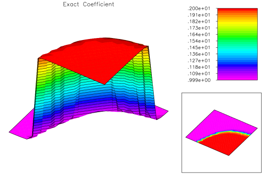
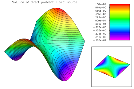
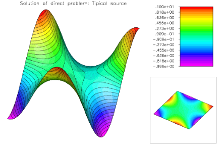
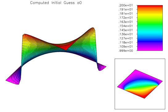
Figure 1: Setup of the inverse doping problem. Top: Parameter function $\gamma^{*}$ to be identified; Center: Functions $U_{1}$ and $U_{6}$ (the Dirichlet boundary conditions at $\partial\Omega$ for (20)) and the solutions $\hat{u}_{2}$, $\hat{u}_{6}$ of the corresponding PDE’s; Bottom: Initial guess $\gamma_{0}$ for the iterative methods PLWK, LWK and LWKls.

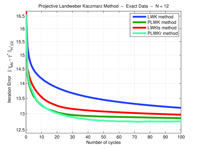
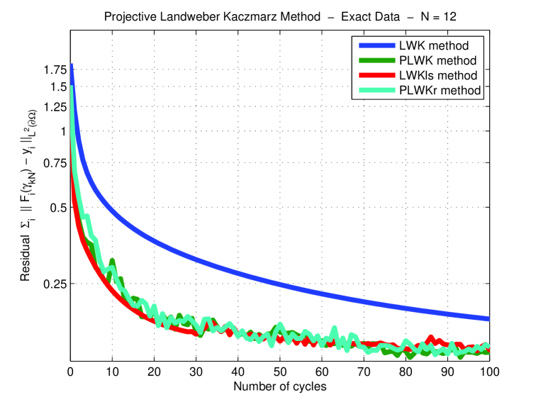
Figure 2: Experiment with exact data. The PLW method (GREEN) is compared with the LW method (BLUE) and with the LWls method (RED). Top: Evolution of the iteration error $\|\gamma_{kN}-\gamma^{\star}\|_{H^{1}(\Omega)}$; Bottom: Evolution of the residual $\textstyle\sum\limits\nolimits_{i=0}^{N-1}\|F_{i}(\gamma_{kN})-y_{i}\|_{L^{2}(\partial\Omega)}$.

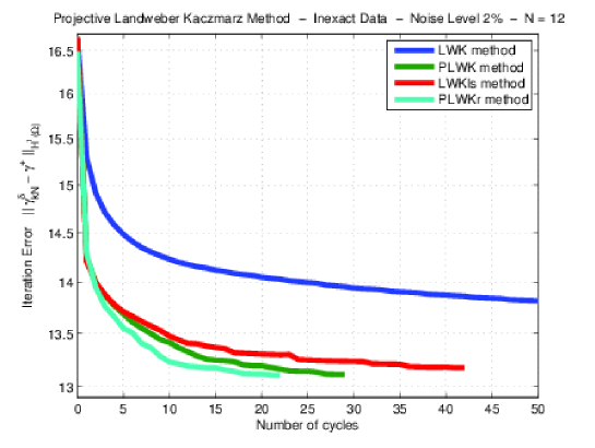
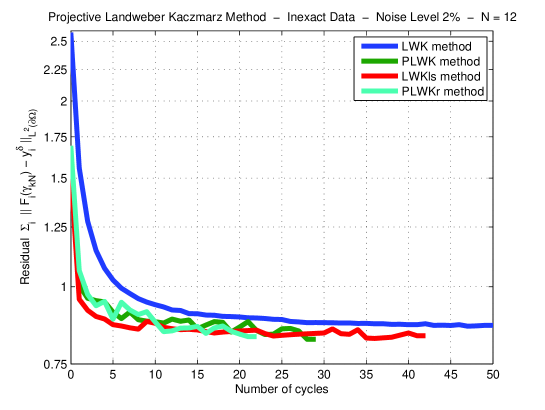
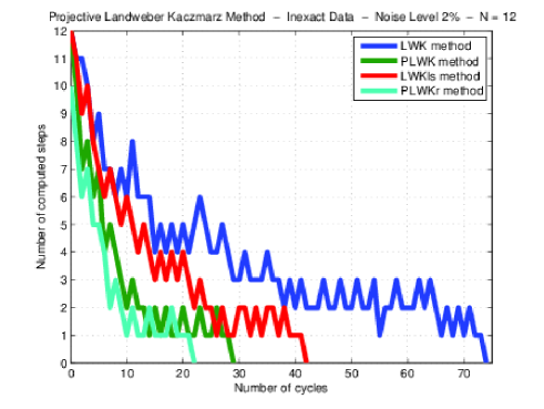
Figure 3: Experiment with noisy data. The PLW method (GREEN) is compared with the LW method (BLUE), the LWls method (RED) and the PLW-random method (LIGHT-BLUE). Top: Evolution of the iteration error; Center: Evolution of the residual Bottom: Number of computed iterative steps per cycle.

Altogether, the PLWK and PLWKr outperformed the other methods in our preliminary numerical experiments. It is worth mentioning that the LWKls, due to the line search, demands in each iteration the solution of three PDE’s, while the other methods require the solution of two PDE’s per iteration. In the noisy data case, very soon many residuals drop bellow the threshold in each cycle, and, in the corresponding iterations, only one PDE has to be solved (see Figure 3).

7 Final remarks and conclusions

In this article we combine the projective Landweber method [24] with Kaczmarz’s method [18] for solving systems of non-linear ill-posed equations.

The underlying assumption used in convergence analysis presented in this manuscript is the tangential cone condition (9). Notice that the convergence analysis of the PLWK method requires $\eta<1$ while the LWK method requires the TCC with $\eta<0.5$ [14].

The numerical experiments depicted in Figure 3 indicate that, in the noisy data case, the bang-bang relaxation parameter $\omega_{k}$ in (6) vanishes for several $k$ (already after the first iterations; see Figure 3 Bottom). Consequently, the computational evaluation of the adjoint $F^{\prime}_{[k]}(x_{k}^{\delta})^{*}$ is avoided, making the PLWK and PLWKr methods a fast alternative to conventional regularization techniques for solving (3) (single equation approach).

The truncation technique used in the Appendix is analogous to the one proposed in [9] to prove a similar result for a steepest-descent type method. The role played by this truncation is merely to provide a sufficient condition for proving strong convergence of the PLWK method. In the realistic noisy data case, this truncation does not modify the original PLWK method introduced in Section 3, whenever the constant $\lambda_{max}$ is chosen large enough.

The PLWK and PLWKr methods have proven to be efficient alternatives to the LWK and LWKls methods for solving ill-posed systems. Comparison with Newton type methods will be the subject of future work.

Appendix A ​​​​​​ppendix: Strong convergence for exact data

In what follows we consider the PLWK iteration in (5) with $\omega_{k}$ defined as in (6), and $\tau$, $p_{i}$ defined as in (12). However, differently from (12), $\lambda_{k}$ is now defined by

$$\lambda_{k}:=\Lambda\Big{(}\dfrac{p_{[k]}(\|F_{[k],\delta}(x_{k}^{\delta})\|)}{\|F_{[k]}^{\prime}(x_{k}^{\delta})^{*}F_{[k],\delta}(x_{k}^{\delta})\|^{2}}\Big{)},\ {\rm if}\ F_{[k]}^{\prime}(x_{k}^{\delta})^{*}F_{[k],\delta}(x_{k}^{\delta})\neq 0,\quad\quad\lambda_{k}:=0,\ {\rm otherwise.}$$ (23)

Here $\Lambda:\mathbb{R}^{+}\to\mathbb{R}$ is a truncation function satisfying $\Lambda(t)=\min\{t,\lambda_{max}\}$ for $t\geq 0$, where $\lambda_{max}>(1-\eta)C^{-2}$ is some positive constant.

In the exact data case we have

$$p_{i}(t)\ :=\ (1-\eta)\,t^{2},\ \ i\in\{0,\dots,N-1\}\quad\quad{\rm and}\quad\quad\omega_{k}\ :=\ \begin{cases}1&F_{[k],0}(x_{k})\neq 0\\ 0&\text{otherwise}\end{cases},\ \ k\in\mathbb{N}.$$

Moreover, we have either $\lambda_{k}=0$ (whenever $F_{[k],0}(x_{k})=0$) or

$$\lambda_{k}\ :=\ \min\Big{\{}\dfrac{(1-\eta)\|F_{[k],0}(x_{k})\|^{2}}{\|F_{[k]}^{\prime}(x_{k})^{*}F_{[k],0}(x_{k})\|^{2}}\,,\ \lambda_{max}\Big{\}}\ >\ \frac{(1-\eta)}{C^{2}}\ =:\ \lambda_{min}.$$ (24)

The inequality in (24) follows from the fact that $x_{k}\in B_{\rho}(x_{0})$ for $k\geq 0$, together with assumption A1 (notice that both Proposition 3.4 and Theorem 3.5 remain valid for PLWK with the new definition of $\lambda_{k}$ in (23)).

In the next theorem we use this setup to prove a strong convergence result for the PLWK iteration in the case of exact data. The truncation function $\Lambda$ is essential for obtaining the estimate (28).

Theorem A.1 (Strong convergence for exact data).

Let assumptions A1 – A3 hold true, $\delta_{0}=\dots=\delta_{N-1}=0$ and $(x_{k})$ be defined by the PLWK method in (5), (6) with $\lambda_{k}$ defined as in (23). If  $\inf$ $\theta_{k}>0$  and  $\sup$ $\theta_{k}<2$, then $(x_{k})$ converges strongly to some $\bar{x}\in B_{\rho}(x_{0})$ solving (2).

Proof.

We define $e_{k}:=x^{\star}-x_{k}$. Since we have exact data, it follows from Proposition 3.4 that $\|e_{k}\|$ is monotone non-increasing. Thus, $\|e_{k}\|$ converges to some $\epsilon\geq 0$. In the following we show that the sequence $(e_{k})$ is a Cauchy sequence. In order to prove this fact, it suffices to show that

$$|\langle e_{l}-e_{k},e_{l}\rangle|\to 0\quad\quad{\rm and}\quad\quad|\langle e_{l}-e_{j},e_{l}\rangle|\to 0$$ (25)

as $k$, $j\to\infty$, where $k\leq j$ and $l\in\{k,\dots,j\}$ (see, e.g., [15, Theorem 2.3] for the Landweber method or [14, Theorem 2.3] for the LWK method).

Let $k\leq j$ be arbitrary. Define  $k_{0}:=\lfloor k/N\rfloor$, $j_{0}:=\lfloor j/N\rfloor$ and  $k_{1}:=[k]$, $j_{1}:=[j]$. Consequently,  $k=k_{0}N+k_{1}$,  $j=j_{0}N+j_{1}$. Now, choose $l_{0}\in\{k_{0},\dots,j_{0}\}$ such that

$$\textstyle\sum\limits_{n=0}^{N-1}\,\|F_{n,0}(x_{l_{0}N+n})\|\ \leq\ \textstyle\sum\limits_{n=0}^{N-1}\,\|F_{n,0}(x_{i_{0}N+n})\|$$ (26)

for all $i_{0}\in\{k_{0},\ldots,j_{0}\}$,  and set $l:=l_{0}N+N-1$. Therefore,

$$|\langle e_{l}-e_{j},e_{l}\rangle|\,=\,\Big{|}\textstyle\sum\limits_{i=l}^{j-1}\langle(x_{i+1}-x_{i}),(x^{\star}-x_{l})\rangle\Big{|}\,=\,\Big{|}\textstyle\sum\limits_{i=l}^{j-1}\theta_{i}\,\lambda_{i}\,\langle y_{[i]}-F_{[i]}(x_{i}),F_{[i]}^{\prime}(x_{i})(x^{\star}-x_{l})\rangle\Big{|}$$ (27)

$$\leq \textstyle\sum\limits_{i=l}^{j-1}\theta_{i}\,\lambda_{i}\,\|F_{[i],0}(x_{i})\|\,\|F_{[i]}^{\prime}(x_{i})(x^{\star}-x_{i})\,+\,F_{[i]}^{\prime}(x_{i})(x_{i}-x_{l})\|$$

$$\leq 2\,\textstyle\sum\limits_{i=l}^{j-1}\lambda_{i}\,\|F_{[i],0}(x_{i})\|\,(1+\eta)\,\Big{[}\|F_{[i]}(x^{\star})-F_{[i]}(x_{i})\|\,+\,\|F_{[i]}(x_{i})-F_{[i]}(x_{l})\|\Big{]}$$

$$= 2\,(1+\eta)\,\textstyle\sum\limits_{i=l}^{j-1}\lambda_{i}\,\|F_{[i],0}(x_{i})\|\,\Big{[}\|F_{[i],0}(x_{i})\|+\|F_{[i]}(x_{i})-y_{[i]}+y_{[i]}-F_{[i]}(x_{l})\|\Big{]}$$

$$\leq 2\,(1+\eta)\textstyle\sum\limits_{i=l}^{j-1}\lambda_{i}\,\|F_{[i],0}(x_{i})\|\,\Big{[}2\|F_{[i],0}(x_{i})\|\,+\,\|F_{[i]}(x_{l})-y_{[i]}\|\Big{]}$$

$$= 4\,(1+\eta)\textstyle\sum\limits_{i=l}^{j-1}\lambda_{i}\,\|F_{[i],0}(x_{i})\|^{2}\ +\ 2\,(1+\eta)\textstyle\sum\limits_{i=l}^{j-1}\lambda_{i}\,\|F_{[i],0}(x_{i})\|\,\|F_{[i],0}(x_{l})\|$$

(in the second inequality we used Proposition 2.1, item 1). Next we estimate the term $\|F_{[i],0}(x_{l})\|$ on the right hand side of (27) (to simplify the notation we write $i=i_{0}N+i_{1}$, with $i_{i}\in\{0,\dots,N-1\}$).

$$\|F_{[i],0}(x_{l})\|\ =\ \|F_{[i]}(x_{l})-y_{[i]}\|\ =\ \|F_{i_{1}}(x_{l_{0}N+N-1})-y_{i_{1}}\|\ \leq$$ (28)

$$\leq \|F_{i_{1}}(x_{l_{0}N+i_{1}})-y_{i_{1}}\|\ +\ \textstyle\sum\limits_{n=i_{1}}^{N-2}\|F_{i_{1}}(x_{l_{0}N+n+1})-F_{i_{1}}(x_{l_{0}N+n})\|$$

$$\leq \|F_{i_{1},0}(x_{l_{0}N+i_{1}})\|\ +\ \frac{1}{(1-\eta)}\,\textstyle\sum\limits_{n=i_{1}}^{N-2}\|F^{\prime}_{i_{1}}(x_{l_{0}N+n})(x_{l_{0}N+n+1}-x_{l_{0}N+n})\|$$

$$\leq \|F_{i_{1},0}(x_{l_{0}N+i_{1}})\|\ +\ \frac{C}{(1-\eta)}\,\textstyle\sum\limits_{n=i_{1}}^{N-2}\|x_{l_{0}N+n+1}-x_{l_{0}N+n}\|$$

$$\leq \|F_{i_{1},0}(x_{l_{0}N+i_{1}})\|\ +\ \frac{C}{(1-\eta)}\,\textstyle\sum\limits_{n=i_{1}}^{N-2}\theta_{l_{0}N+n}\,\lambda_{l_{0}N+n}\,\|F_{n}^{\prime}(x_{l_{0}N+n})^{*}F_{n,0}(x_{l_{0}N+n})\|$$

$$\leq \|F_{i_{1},0}(x_{l_{0}N+i_{1}})\|\ +\ \frac{2C^{2}}{(1-\eta)}\,\textstyle\sum\limits_{n=i_{1}}^{N-2}\lambda_{max}\,\|F_{n,0}(x_{l_{0}N+n})\|$$

$$\leq \widetilde{C}\,\textstyle\sum\limits_{n=i_{1}}^{N-2}\|F_{n,0}(x_{l_{0}N+n})\|\ \leq\ \widetilde{C}\,\textstyle\sum\limits_{n=0}^{N-1}\|F_{n,0}(x_{l_{0}N+n})\|$$

(the second inequality follows from Proposition 2.1, item 1). Here $\widetilde{C}=\big{[}2(1-\eta)+4C^{2}\lambda_{max}\big{]}\,(1-\eta)^{-1}$. Using (28) we estimate the second sum on the right hand side of (27) (once again we adopt the notation $i=i_{0}N+i_{1}$).

$$\textstyle\sum\limits_{i=l}^{j-1}\lambda_{i}\,\|F_{[i],0}(x_{i})\|\,\|F_{[i],0}(x_{l})\|\ \leq\ \textstyle\sum\limits_{i_{0}=l_{0}}^{j_{0}}\ \textstyle\sum\limits_{i_{1}=0}^{N-1}\lambda_{i}\,\|F_{i_{1},0}(x_{i})\|\,\|F_{i_{1},0}(x_{l})\|$$ (29)

$$\leq \textstyle\sum\limits_{i_{0}=l_{0}}^{j_{0}}\,\Big{[}\,\textstyle\sum\limits_{i_{1}=0}^{N-1}\,\lambda_{i}\,\|F_{i_{1},0}(x_{i})\|\,\Big{(}\widetilde{C}\textstyle\sum\limits_{n=0}^{N-1}\,\|F_{n,0}(x_{l_{0}N+n})\|\Big{)}\Big{]}$$

$$\leq \widetilde{C}\,\lambda_{max}\,\textstyle\sum\limits_{i_{0}=l_{0}}^{j_{0}}\,\Big{(}\textstyle\sum\limits_{i_{1}=0}^{N-1}\|F_{i_{1},0}(x_{i_{0}N+i_{1}})\|\Big{)}\,\Big{(}\textstyle\sum\limits_{n=0}^{N-1}\,\|F_{n,0}(x_{l_{0}N+n})\|\Big{)}$$

$$\leq \widetilde{C}\,\lambda_{max}\,\textstyle\sum\limits_{i_{0}=l_{0}}^{j_{0}}\,\Big{(}\textstyle\sum\limits_{i_{1}=0}^{N-1}\|F_{i_{1},0}(x_{i_{0}N+i_{1}})\|\Big{)}^{2}$$

$$\leq \widetilde{C}\,\lambda_{max}\,\textstyle\sum\limits_{i_{0}=l_{0}}^{j_{0}}N\,\textstyle\sum\limits_{i_{1}=0}^{N-1}\|F_{i_{1},0}(x_{i_{0}N+i_{1}})\|^{2}$$

$$= \widetilde{C}\,N\,\lambda_{max}\textstyle\sum\limits_{i=l_{0}}^{j_{0}N+N-1}\,\|F_{[i],0}(x_{i})\|^{2},$$

where the third inequality follows from (26). Substituting (29) in (27) we obtain

$$|\langle e_{l}-e_{j},e_{l}\rangle| \leq 4(1+\eta)\lambda_{max}\textstyle\sum\limits_{i=l}^{j-1}\|F_{[i],0}(x_{i})\|^{2}\ +\ 2(1+\eta)\widetilde{C}N\lambda_{max}\!\!\textstyle\sum\limits_{i=l_{0}}^{j_{0}N+N-1}\,\|F_{[i],0}(x_{i})\|^{2}$$

$$\leq \widetilde{\!\widetilde{C}}\,\textstyle\sum\limits_{i=l_{0}}^{\infty}\,\lambda_{i}\,\|F_{[i],0}(x_{i})\|^{2},$$

where $\widetilde{\!\widetilde{C}}=2\lambda_{max}\,(1+\eta)\,[2+\widetilde{C}N]\,\lambda_{min}^{-1}$ (in the last inequality we used (24)).

From (17) and the definition of the index $l\in\{k,\dots,j\}$ it follows that, given $\epsilon>0$ there exists some $N_{\epsilon}\in\mathbb{N}$ such that $|\langle e_{l}-e_{j},e_{l}\rangle|\leq\epsilon/2$ for $k$, $j\geq N_{\epsilon}$. Analogously, one shows that $|\langle e_{l}-e_{k},e_{l}\rangle|\leq\epsilon$ for $k$, $j\geq N_{\epsilon}$. This is sufficient to guarantee (25).

Consequently, $x_{k}=x^{\star}-e_{k}$ converges to some $\bar{x}\in B_{\rho}(x_{0})$. Since, due to (17), the residuals $\|F_{[k],0}(x_{k})\|$ converge to zero as $k\to\infty$, we conclude that $\bar{x}$ is a solution of (2), completing the proof. ∎

References

- [1] A.B. Bakushinsky and M.Y. Kokurin. Iterative Methods for Approximate Solution of Inverse Problems, volume 577 of Mathematics and Its Applications. Springer, Dordrecht, 2004.
- [2] Randolph E. Bank. PLTMG: a software package for solving elliptic partial differential equations, volume 15 of Frontiers in Applied Mathematics. Society for Industrial and Applied Mathematics (SIAM), Philadelphia, PA, 1994. Users’ guide 7.0.
- [3] J. Baumeister, B. Kaltenbacher, and A. Leitão. On levenberg-marquardt-kaczmarz iterative methods for solving systems of nonlinear ill-posed equations. Inverse Probl. Imaging, 4(3):335–350, 2010.
- [4] H.H.. Bauschke and J.M. Borwein. Legendre functions and the method of random bregman projections. Journal of Convex Analysis, 4(1):27–67, 1997.
- [5] M. Burger, H. W. Engl, A. Leitão, and P.A. Markowich. On inverse problems for semiconductor equations. Milan J. Math., 72:273–313, 2004.
- [6] M. Burger and B. Kaltenbacher. Regularizing Newton-Kaczmarz methods for nonlinear ill-posed problems. SIAM J. Numer. Anal., 44:153–182, 2006.
- [7] C.L. Byrne. Signal processing. Monographs and Research Notes in Mathematics. CRC Press, Boca Raton, FL, second edition, 2015. A mathematical approach.
- [8] M. Cullen, M.A. Freitag, S. Kindermann, and R. Scheichl, editors. Large Scale Inverse Problems, volume 13 of Radon Series on Computational and Applied Mathematics. De Gruyter, Berlin, 2013. Computational methods and applications in the earth sciences.
- [9] A. De Cezaro, M. Haltmeier, A. Leitão, and O. Scherzer. On steepest-descent-Kaczmarz methods for regularizing systems of nonlinear ill-posed equations. Appl. Math. Comput., 202(2):596–607, 2008.
- [10] H.W. Engl, M. Hanke, and A. Neubauer. Regularization of Inverse Problems. Kluwer Academic Publishers, Dordrecht, 1996.
- [11] C. W. Groetsch. Stable Approximate Evaluation of Unbounded Operators, volume 1894 of Lecture Notes in Mathematics. Springer-Verlag, Berlin, 2007.
- [12] M. Haltmeier, R. Kowar, A. Leitão, and O. Scherzer. Kaczmarz methods for regularizing nonlinear ill-posed equations. II. Applications. Inverse Probl. Imaging, 1(3):507–523, 2007.
- [13] M. Haltmeier, A. Leitão, and E. Resmerita. On regularization methods of EM-Kaczmarz type. Inverse Problems, 25:075008, 2009.
- [14] M. Haltmeier, A. Leitão, and O. Scherzer. Kaczmarz methods for regularizing nonlinear ill-posed equations. I. convergence analysis. Inverse Probl. Imaging, 1(2):289–298, 2007.
- [15] M. Hanke, A. Neubauer, and O. Scherzer. A convergence analysis of Landweber iteration for nonlinear ill-posed problems. Numerische Mathematik, 72:21–37, 1995.
- [16] G. T. Herman. A relaxation method for reconstructing objects from noisy X-rays. Math. Programming, 8:1–19, 1975.
- [17] Gabor T. Herman. Image reconstruction from projections. Academic Press, Inc. [Harcourt Brace Jovanovich, Publishers], New York-London, 1980. The fundamentals of computerized tomography, Computer Science and Applied Mathematics.
- [18] S. Kaczmarz. Angenäherte auflösung von systemen linearer gleichungen. Bull. International de l’Academie Polonaise des Sciences. Lett A, pages 355–357, 1937.
- [19] B. Kaltenbacher, A. Neubauer, and O. Scherzer. Iterative regularization methods for nonlinear ill-posed problems, volume 6 of Radon Series on Computational and Applied Mathematics. Walter de Gruyter GmbH & Co. KG, Berlin, 2008.
- [20] L. Landweber. An iteration formula for Fredholm integral equations of the first kind. Amer. J. Math., 73:615–624, 1951.
- [21] A. Lechleiter and A. Rieder. Newton regularizations for impedance tomography: convergence by local injectivity. Inverse Problems, 24(6), 2008.
- [22] A. Leitão. Semiconductors and Dirichlet-to-Neumann maps. Comput. Appl. Math., 25(2-3):187–203, 2006.
- [23] A. Leitão, P.A. Markowich, and J.P. Zubelli. Inverse Problems for Semiconductors: Models and Methods, chapter in Transport Phenomena and Kinetic Theory: Applications to Gases, Semiconductors, Photons, and Biological Systems, Ed. C.Cercignani and E.Gabetta. Birkhäuser, Boston, 2006.
- [24] A. Leitão and B.F. Svaiter. Projective acceleration of the nonlinear Landweber method under the tangential cone condition. (submitted), 2015.
- [25] F. Margotti, A. Rieder, and A. Leitão. A Kaczmarz version of the reginn-Landweber iteration for ill-posed problems in Banach spaces. SIAM J. Numer. Anal., 52(3):1439–1465, 2014.
- [26] V.A. Morozov. Regularization Methods for Ill–Posed Problems. CRC Press, Boca Raton, 1993.
- [27] F. Natterer. Regularisierung schlecht gestellter Probleme durch Projektionsverfahren. Numerische Mathematik, 28(3):329–341, 1977.
- [28] F. Natterer. The Mathematics of Computerized Tomography. B.G. Teubner, Stuttgart; John Wiley & Sons, Ltd., Chichester, 1986.
- [29] F. Natterer. Algorithms in tomography. In State of the art in numerical analysis, volume 63, pages 503–524, 1997.
- [30] F. Natterer and F. Wübbeling. Mathematical Methods in Image Reconstruction. SIAM, Philadelphia, 2001.
- [31] Zdzisław Opial. Weak convergence of the sequence of successive approximations for nonexpansive mappings. Bull. Amer. Math. Soc., 73:591–597, 1967.
- [32] H.A. Sabbagh, R.K. Murphy, E.H. Sabbagh, J.C. Aldrin, and J.S. Knopp. Computational electromagnetics and model-based inversion. Scientific Computation. Springer, New York, 2013. A modern paradigm for eddy-current nondestructive evaluation.
- [33] O. Scherzer. Convergence rates of iterated Tikhonov regularized solutions of nonlinear ill-posed problems. Numerische Mathematik, 66(2):259–279, 1993.
- [34] F. Schöpfer, T. Schuster, and A.K. Louis. An iterative regularization method for the solution of the split feasibility problem in banach spaces. Inverse Problems, 24(5):055008, 2008.
- [35] T.I. Seidman and C.R. Vogel. Well posedness and convergence of some regularisation methods for non–linear ill posed problems. Inverse Probl., 5:227–238, 1989.
- [36] A.N. Tikhonov. Regularization of incorrectly posed problems. Soviet Math. Dokl., 4:1624–1627, 1963.
- [37] A.N. Tikhonov and V.Y. Arsenin. Solutions of Ill-Posed Problems. John Wiley & Sons, Washington, D.C., 1977. Translation editor: Fritz John.
- [38] M. Vetterli, J. Kovacevic, and V.K. Goyal. Foundations of Signal Processing. Cambridge University Press, Cambridge, 2014. A modern paradigm for eddy-current nondestructive evaluation.