CRPO: A New Approach for Safe Reinforcement Learning with Convergence Guarantee

Abstract

In safe reinforcement learning (SRL) problems, an agent explores the environment to maximize an expected total reward and meanwhile avoids violation of certain constraints on a number of expected total costs. In general, such SRL problems have nonconvex objective functions subject to multiple nonconvex constraints, and hence are very challenging to solve, particularly to provide a globally optimal policy. Many popular SRL algorithms adopt a primal-dual structure which utilizes the updating of dual variables for satisfying the constraints. In contrast, we propose a primal approach, called constraint-rectified policy optimization (CRPO), which updates the policy alternatingly between objective improvement and constraint satisfaction. CRPO provides a primal-type algorithmic framework to solve SRL problems, where each policy update can take any variant of policy optimization step. To demonstrate the theoretical performance of CRPO, we adopt natural policy gradient (NPG) for each policy update step and show that CRPO achieves an $\mathcal{O}(1/\sqrt{T})$ convergence rate to the global optimal policy in the constrained policy set and an $\mathcal{O}(1/\sqrt{T})$ error bound on constraint satisfaction. This is the first finite-time analysis of primal SRL algorithms with global optimality guarantee. Our empirical results demonstrate that CRPO can outperform the existing primal-dual baseline algorithms significantly.

1 Introduction

Reinforcement learning (RL) has achieved great success in solving complex sequential decision-making and control problems such as Go (Silver et al., 2017), StarCraft (DeepMind, 2019) and recommendation system (Zheng et al., 2018), etc. In these settings, the agent is allowed to explore the entire state and action space to maximize the expected total reward. However, in safe RL (SRL), in addition to maximizing the reward, an agent needs to satisfy certain constraints. Examples include self-driving cars (Fisac et al., 2018), cellular network (Julian et al., 2002), and robot control (Levine et al., 2016). The global optimal policy in SRL is the one that maximizes the reward and at the same time satisfies the cost constraints.

The current safe RL algorithms can be generally categorized into the primal and primal-dual approaches. The primal-dual approaches (Tessler et al., 2018; Ding et al., 2020a; Stooke et al., 2020; Yu et al., 2019; Achiam et al., 2017; Yang et al., 2019a; Altman, 1999; Borkar, 2005; Bhatnagar & Lakshmanan, 2012; Liang et al., 2018; Paternain et al., 2019a) are most commonly used, which convert the constrained problem into an unconstrained one by augmenting the objective with a sum of constraints weighted by their corresponding Lagrange multipliers (i.e., dual variables). Generally, primal-dual algorithms apply a certain policy optimization update such as policy gradient alternatively with a gradient descent type update for the dual variables. Theoretically, (Tessler et al., 2018) has provided an asymptotic convergence analysis for primal-dual method and established a local convergence guarantee. (Paternain et al., 2019b) showed that the primal-dual method achieves zero duality gap. Recently, (Ding et al., 2020a) proposed a primal-dual type proximal policy optimization (PPO) and established the regret bound for linear constrained MDP. The convergence rate of primal-dual method based on a natural policy gradient algorithm was characterized in (Ding et al., 2020b).

The primal type of approaches (Liu et al., 2019b; Chow et al., 2018, 2019; Dalal et al., 2018a) enforce constraints via various designs of the objective function or the update process without an introduction of dual variables. The primal algorithms are much less studied than the primal-dual approach. Notably, (Liu et al., 2019b) developed an interior point method, which applies logarithmic barrier functions for SRL. (Chow et al., 2018, 2019) leveraged Lyapunov functions to handle constraints. (Dalal et al., 2018a) introduced a safety layer to the policy network to enforce constraints. None of the existing primal algorithms are shown to have provable convergence guarantee to a globally optimal feasible policy.

Comparing between the primal-dual and primal approaches, the primal-dual approach can be sensitive to the initialization of Lagrange multipliers and the learning rate, and can thus incur extensive cost in hyperparameter tuning (Achiam et al., 2017; Chow et al., 2019). In contrast, the primal approach does not introduce additional dual variables to optimize and involves less hyperparamter tuning, and hence holds the potential to be much easier to implement than the primal-dual approach. However, the existing primal algorithms are not yet popular in practice so far, because of no guaranteed global convergence and no strong demonstrations to have competing performance as the primal-dual algorithms. Thus, in order to take the advantage of the primal approach which is by nature easier to implement, we need to answer the following fundamental questions.

• Can we design a primal algorithm for SRL, and demonstrate that it achieves competing performance or outperforms the baseline primal-dual approach?

• If so, can we establish global optimality guarantee and the finite-time convergence rate for the proposed primal algorithm?

In this paper, we will provide the affirmative answers to the above questions, thus establishing appealing advantages of the primal approach for SRL.

1.1 Main Contributions

A New Algorithm: We propose a novel primal approach called Constraint-Rectified Policy Optimization (CRPO) for SRL, where all updates are taken in the primal domain. CRPO applies unconstrained policy maximization update w.r.t. the reward on the one hand, and if any constraint is violated, momentarily rectifies the policy back to the constraint set along the descent direction of the violated constraint also by applying unconstrained policy minimization update w.r.t. the constraint function. From the implementation perspective, CRPO can be implemented as easy as unconstrained policy optimization algorithms. Without introduction of dual variables, it does not suffer from hyperparameter tuning of the learning rates to which the dual variables are sensitive, nor does it require initialization to be feasible. Further, CRPO involves only policy gradient descent for both objective and constraints, whereas the primal-dual approach typically requires projected gradient descent, where the projection causes higher complexity to implementation as well as hyperparameter tuning due to the projection thresholds.

To further explain the advantage of CRPO over the primal-dual approach, CRPO features immediate switches between optimizing the objective and reducing the constraints whenever constraints are violated. However, the primal-dual approach can respond much slower because the control is based on dual variables. If a dual variable is nonzero, then the policy update will descend along the corresponding constraint function. As a result, even if a constraint is already satisfied, there can often be a significant delay for the dual variable to iteratively reduce to zero to release the constraint, which slows down the algorithm. Our experiments in Section 5 validates such a performance advantage of CRPO over the primal-dual approach.

Theoretical Guarantee: To provide the theoretical guarantee for CRPO, we adopt NPG as a representative policy optimizer and investigate the convergence of CRPO in two settings: tabular and function approximation, where in the function approximation setting the state space can be infinite. For both settings, we show that CRPO converges to a global optimum at a convergence rate of $\mathcal{O}(1/\sqrt{T})$. Furthermore, the constraint violation also converges to zero at a rate of $\mathcal{O}(1/\sqrt{T})$. To the best of our knowledge, we establish the first provably global optimality guarantee for a primal SRL algorithm of CRPO.

To compare with the primal-dual approach in the function approximation setting, the value function gap of CRPO achieves the same convergence rate as the primal-dual approach, but the constraint violation of CRPO decays at a rate of $\mathcal{O}(1/\sqrt{T})$, which is much faster than the rate $\mathcal{O}(1/T^{\frac{1}{4}})$ of the primal-dual approach (Ding et al., 2020b).

Technically, our analysis has the following novel developments. (a) We develop a new technique to analyze a stochastic approximation (SA) that randomly and dynamically switches between the target objectives of the reward and the constraint. Such an SA by nature is different from the analysis of a typical policy optimization algorithm, which has a fixed target objective to optimize. Our analysis constructs novel concentration events for capturing the impact of such a dynamic process on the update of the reward and cost functions in order to establish the high probability convergence guarantee. (b) We also develop new tools to handle multiple constraints, which is particularly non-trivial for our algorithm that involves stochastic selection of a constraint if multiple constraints are violated.

1.2 Related Work

Safe RL: Algorithms based on primal-dual methods have been widely adopted for solving constrained RL problems, such as PDO (Chow et al., 2017), RCPO (Tessler et al., 2018), OPDOP (Ding et al., 2020a) and CPPO (Stooke et al., 2020). Constrained policy optimization (CPO) (Achiam et al., 2017) extends TRPO to handle constraints, and is later modified with a two-step projection method (Yang et al., 2019a). The effectiveness of primal-dual methods is justified in (Paternain et al., 2019b), in which zero duality gap is guaranteed under certain assumptions. A recent work (Ding et al., 2020b) established the convergence rate of the primal-dual method under Slater’s condition assumption. Other methods have also been proposed. For example, (Chow et al., 2018, 2019) leveraged Lyapunov functions to handle constraints. (Yu et al., 2019) proposed a constrained policy gradient algorithm with convergence guarantee by solving a sequence of sub-problems. (Dalal et al., 2018a) proposed to add a safety layer to the policy network so that constraints can be satisfied at each state. (Liu et al., 2019b) developed an interior point method for safe RL, which augments the objective with logarithmic barrier functions. Our work proposes a CRPO algorithm, which can be implemented as easy as unconstrained policy optimization methods and has global optimality guarantee under general constrained MDP. Our result is the first convergence rate characterization of primal-type algorithms for SRL.

Finite-Time Analysis of Policy Optimization: The finite-time analysis of various policy optimization algorithms under unconstrained MDPs have been well studied. The convergence rate of policy gradient (PG) and actor-critic (AC) algorithms have been established in (Shen et al., 2019; Papini et al., 2017, 2018; Xu et al., 2020a, 2019a; Xiong et al., 2020; Zhang et al., 2019) and (Xu et al., 2020b; Wang et al., 2019; Yang et al., 2019b; Kumar et al., 2019; Qiu et al., 2019), respectively, in which PG or AC algorithm is shown to converge to a local optimal. In some special settings such as tabular and LQR, PG and AC can be shown to convergence to the global optimal (Agarwal et al., 2019; Yang et al., 2019b; Fazel et al., 2018; Malik et al., 2018; Tu & Recht, 2018; Bhandari & Russo, 2019, 2020). Algorithms such as NPG, NAC, TRPO and PPO explore the second order information, and achieve great success in practice. These algorithms have been shown to converge to a global optimum in various settings, where the convergence rate has been established in (Agarwal et al., 2019; Shani et al., 2019; Liu et al., 2019a; Wang et al., 2019; Cen et al., 2020; Xu et al., 2020c).

2 Problem Formulation and Preliminaries

2.1 Markov Decision Process

A discounted Markov decision process (MDP) is a tuple $(\mathcal{S},\mathcal{A},c_{0},\mathsf{P},\xi,\gamma)$, where $\mathcal{S}$ and $\mathcal{A}$ are state and action spaces; $c_{0}:\mathcal{S}\times\mathcal{A}\times\mathcal{S}\rightarrow{\mathbb{R}}$ is the reward function; $\mathsf{P}:\mathcal{S}\times\mathcal{A}\times\mathcal{S}\rightarrow[0,1]$ is the transition kernel, with $\mathsf{P}(s^{\prime}|s,a)$ denoting the probability of transitioning to state $s^{\prime}$ from previous state $s$ given action $a$; $\xi:\mathcal{S}\rightarrow[0,1]$ is the initial state distribution; and $\gamma\in(0,1)$ is the discount factor. A policy $\pi:\mathcal{S}\rightarrow{\mathcal{P}}(\mathcal{A})$ is a mapping from the state space to the space of probability distributions over the actions, with $\pi(\cdot|s)$ denoting the probability of selecting action $a$ in state $s$. When the associated Markov chain $\mathsf{P}(s^{\prime}|s)=\sum_{\mathcal{A}}P(s^{\prime}|s,a)\pi(a|s)$ is ergodic, we denote $\mu_{\pi}$ as the stationary distribution of this MDP, i.e. $\int_{\mathcal{S}}\mathsf{P}(s^{\prime}|s)\mu_{\pi}(ds)=\mu_{\pi}(s^{\prime})$. Moreover, we define the visitation measure induced by the police $\pi$ as $\nu_{\pi}(s,a)=(1-\gamma)\sum_{t=0}^{\infty}\gamma^{t}\mathsf{P}(s_{t}=s,a_{t}=a)$.

For a given policy $\pi$, we define the state value function as $V^{0}_{\pi}(s)={\mathbb{E}}[\sum_{t=0}^{\infty}\gamma^{t}c_{0}(s_{t},a_{t},s_{t+1})|s_{0}=s,\pi]$, the state-action value function as $Q^{0}_{\pi}(s,a)={\mathbb{E}}[\sum_{t=0}^{\infty}\gamma^{t}c_{0}(s_{t},a_{t},s_{t+1})|s_{0}=s,a_{0}=a,\pi]$, and the advantage function as $A^{0}_{\pi}(s,a)=Q^{0}_{\pi}(s,a)-V^{0}_{\pi}(s)$. In reinforcement learning, we aim to find an optimal policy that maximizes the expected total reward function defined as $J_{0}(\pi)={\mathbb{E}}[\sum_{t=0}^{\infty}\gamma^{t}c_{0}(s_{t},a_{t},s_{t+1})]={\mathbb{E}}_{\xi}[V^{0}_{\pi}(s)]={\mathbb{E}}_{\xi\cdot\pi}[Q^{0}_{\pi}(s,a)]$.

2.2 Safe Reinforcement Learning (SRL) Problem

The SRL problem is formulated as an MDP with additional constraints that restrict the set of allowable policies. Specifically, when taking action at some state, the agent can incur a number of costs denoted by $c_{1},\cdots,c_{p}$, where each cost function $c_{i}:\mathcal{S}\times\mathcal{A}\times\mathcal{S}\rightarrow{\mathbb{R}}$ maps a tuple $(s,a,s^{\prime})$ to a cost value. Let $J_{i}(\pi)$ denotes the expected total cost function with respect to $c_{i}$ as $J_{i}(\pi)={\mathbb{E}}[\sum_{t=0}^{\infty}\gamma^{t}c_{i}(s_{t},a_{t},s_{t+1})]$. The goal of the agent in SRL is to solve the following constrained problem

$$\max\limits_{\pi}J_{0}(\pi),\,\,\,\text{s.t.}\,\,\,J_{i}(\pi)\leq d_{i},\,\,\forall i=1,\cdots,p,$$ (1)

where $d_{i}$ is a fixed limit for the $i$-th constraint. We denote the set of feasible policies as $\Omega_{C}\equiv\{\pi:\forall i,J_{i}(\pi)\leq d_{i}\}$, and define the optimal policy for SRL as $\pi^{*}=\operatorname*{arg\,min}_{\pi\in\Omega_{C}}J_{0}(\pi)$. For each cost $c_{i}$, we define its corresponding state value function $V^{i}_{\pi}$, state-action value function $Q^{i}_{\pi}$, and advantage function $A^{i}_{\pi}$ analogously to $V^{0}_{\pi}$, $Q^{0}_{\pi}$, and $A^{0}_{\pi}$, with $c_{i}$ replacing $c_{0}$, respectively.

2.3 Policy Parameterization and Policy Gradient

In practice, a convenient way to solve the problem eq. 1 is to parameterize the policy and then optimize the policy over the parameter space. Let $\{\pi_{w}:\mathcal{S}\rightarrow{\mathcal{P}}(\mathcal{A})|w\in{\mathcal{W}}\}$ be a parameterized policy class, where ${\mathcal{W}}$ is the parameter space. Then, the problem in eq. 1 becomes

$$\max\limits_{w\in{\mathcal{W}}}J_{0}(\pi_{w}),\,\,\,\text{s.t.}\,\,\,J_{i}(\pi_{w})\leq d_{i},\,\forall i=1,\cdots,p.$$ (2)

The policy gradient of the function $J_{i}(\pi_{w})$ has been derived by (Sutton et al., 2000) as $\nabla J_{i}(\pi_{w})={\mathbb{E}}[Q^{i}_{\pi_{w}}(s,a)\phi_{w}(s,a)]$, where $\phi_{w}(s,a)\coloneqq\nabla_{w}\log\pi_{w}(a|s)$ is the score function. Furthermore, the natural policy gradient was defined by (Kakade, 2002) as $\Delta_{i}(w)=F(w)^{\dagger}\nabla J_{i}(\pi_{w})$, where $F(w)$ is the Fisher information matrix defined as $F(w)={\mathbb{E}}_{\nu_{\pi_{w}}}[\phi_{w}(s,a)\phi_{w}(s,a)^{\top}]$.

3 Constraint-Rectified Policy Optimization (CRPO) Algorithm

Algorithm 1 Constraint-Rectified Policy Optimization (CRPO)

1:  Initialize: initial parameter $w_{0}$, empty set ${\mathcal{N}}_{0}$

2:  for $t=0,\cdots,T-1$ do

3:    Policy evaluation under $\pi_{w_{t}}$: $\bar{Q}^{i}_{t}(s,a)\approx Q^{i}_{\pi_{w_{t}}}(s,a)$

4:    Sample $(s_{j},a_{j})\in{\mathcal{B}}_{t}\sim\xi\cdot\pi_{w_{t}}$, compute constrain estimation $\bar{J}_{i,{\mathcal{B}}_{t}}=\sum_{j\in{\mathcal{B}}_{t}}\rho_{j,t}\bar{Q}^{i}_{t}(s_{j},a_{j})$ for $i=0,\cdots,p$, ($\rho_{j,t}$ is the weight)

5:    if $\bar{J}_{i,{\mathcal{B}}_{t}}\leq d_{i}+\eta$ for all $i=1,\cdots,p$, then

6:       Add $w_{t}$ into set ${\mathcal{N}}_{0}$

7:       Take one-step policy update towards maximize $J_{0}(w_{t})$: $w_{t}\rightarrow w_{t+1}$

8:    else

9:       Choose any $i_{t}\in\{1,\cdots,p\}$ such that $\bar{J}_{i_{t},{\mathcal{B}}_{t}}>d_{i_{t}}+\eta$

10:       Take one-step policy update towards minimize $J_{i_{t}}(w_{t})$: $w_{t}\rightarrow w_{t+1}$

11:    end if

12:  end for

13:  Output: $w_{\text{out}}$ uniformly chosen from ${\mathcal{N}}_{0}$

In this section, we propose the CRPO approach (see Algorithm 1) for solving the SRL problem in eq. 2. The idea of CRPO lies in updating the policy to maximize the unconstrained objective function $J_{0}(\pi_{w_{t}})$ of the reward, alternatingly with rectifying the policy to reduce a constraint function $J_{i}(\pi_{w_{t}})$ $(i\geq 1)$ (along the descent direction of this constraint) if it is violated. Each iteration of CRPO consists of the following three steps.

Policy Evaluation: At the beginning of each iteration, we estimate the state-action value function $\bar{Q}^{i}_{\pi_{t}}(s,a)\approx{Q}^{i}_{\pi_{w_{t}}}(s,a)$ ($i=\{0,\cdots,p\}$) for both reward and costs under current policy $\pi_{w_{t}}$.

Constraint Estimation: After obtaining $\bar{Q}^{i}_{\pi_{t}}$, the constraint function ${J}_{i}(w_{t})={\mathbb{E}}_{\xi\cdot\pi_{w_{t}}}[Q^{i}_{w_{t}}(s,a)]$ can then be approximated via a weighted sum of approximated state-action value function: $\bar{J}_{i,{\mathcal{B}}_{t}}=\sum_{j\in{\mathcal{B}}_{t}}\rho_{j,t}\bar{Q}^{i}_{t}(s_{j},a_{j})$. Note this step does not take additional sampling cost, as the generation of samples $(s_{j},a_{j})\in{\mathcal{B}}_{t}$ from distribution $\xi\cdot\pi_{w_{t}}$ does not require the agent to interact with the environment.

Policy Optimization: We then check whether there exists an $i_{t}\in\{1,\cdots,p\}$ such that the approximated constraint $\bar{J}_{i_{t},{\mathcal{B}}_{t}}$ violates the condition $\bar{J}_{i_{t},{\mathcal{B}}_{t}}\leq d_{i}+\eta$, where $\eta$ is the tolerance. If so, we take one-step update of the policy towards minimizing the corresponding constraint function $J_{i_{t}}(\pi_{w_{t}})$ to enforce the constraint. If multiple constraints are violated, we can choose to minimize any one of them. If all constraints are satisfied, we take one-step update of the policy towards maximizing the objective function $J_{0}(\pi_{w_{t}})$. To apply CRPO in practice, we can use any policy optimization update such as natural policy gradient (NPG) (Kakade, 2002), trust region policy optimization (TRPO) (Schulman et al., 2015), proximal policy optimization (PPO) (Schulman et al., 2017), ACKTR (Wu et al., 2017), DDPG (Lillicrap et al., 2015) and SAC (Haarnoja et al., 2018), etc, in the policy optimization step (line 7 and line 10).

The advantage of CRPO over the primal-dual approach can be readily seen from its design. CRPO features immediate switches between optimizing the objective and reducing the constraints whenever they are violated. However, the primal-dual approach can respond much slower because the control is based on dual variables. If a dual variable is nonzero, then the policy update will descend along the corresponding constraint function. As a result, even if a constraint is already satisfied, there can still be a delay (sometimes a significant delay) for the dual variable to iteratively reduce to zero to release the constraint, which yields unnecessary sampling cost and slows down the algorithm. Our experiments in Section 5 validates such a performance advantage of CRPO over the primal-dual approach.

From the implementation perspective, CRPO can be implemented as easy as unconstrained policy optimization such as unconstrained policy gradient algorithms, whereas the primal-dual approach typically requires the projected gradient descent to update the dual variables, which is more complex to implement. Further, without introduction of the dual variables, CRPO does not suffer from hyperparameter tuning of the learning rates and projection threshold of the dual variables, whereas the primal-dual approach can be very sensitive to these hyperparamters. Nor does CRPO require initialization to be feasible, whereas the primal-dual approach can suffer significantly from bad initialization. We also empirically verify that the performance of CRPO is robust to the value of $\eta$ over a wide range, which does not cause additional tuning effort compared to unconstrained algorithms. More discussions can be referred to Section 5.

CRPO algorithm is inspired by, yet very different from the cooperative stochastic approximation (CSA) method (Lan & Zhou, 2016) in optimization literature. First, CSA is designed for convex optimization subject to convex constraint, and is not readily capable of handling the more challenging SRL problems eq. 2, which are nonconvex optimization subject to nonconvex constraints. Second, CSA is designed to handle only a single constraint, whereas CRPO can handle multiple constraints with guaranteed constraint satisfaction and global optimality. Thus, the finite-time analysis for CSA and CRPO feature different approaches due to the aforementioned differences in their designs.

4 Convergence Analysis of CRPO

In this section, we take NPG as a representative optimizer in CRPO, and establish the global convergence rate of CRPO in both the tabular and function approximation settings. Note that TRPO and ACKTR update can be viewed as the NPG approach with adaptive stepsize. Thus, the convergence we establish for NPG implies similar results for CRPO that takes TRPO or ACKTR as the optimizer.

4.1 Tabular Setting

In the tabular setting, we consider the softmax parameterization. For any $w\in{\mathbb{R}}^{\left|\mathcal{S}\right|\times\left|\mathcal{A}\right|}$, the corresponding softmax policy $\pi_{w}$ is defined as

$$\pi_{w}(a|s)\coloneqq\frac{\exp(w(s,a))}{\sum_{a^{\prime}\in\mathcal{A}}\exp(w(s,a^{\prime}))},\quad\forall(s,a)\in\mathcal{S}\times\mathcal{A}.$$ (3)

Clearly, the policy class defined in eq. 3 is complete, as any stochastic policy in the tabular setting can be represented in this class.

Policy Evaluation: To perform the policy evaluation in Algorithm 1 (line 3), we adopt the temporal difference (TD) learning, in which a vector $\theta^{i}\in{\mathbb{R}}^{\left|\mathcal{S}\right|\times\left|\mathcal{A}\right|}$ is used to estimate the state-action value function $Q^{i}_{\pi_{w}}$ for all $i=0,\cdots,p$. Specifically, each iteration of TD learning takes the form of

$$\theta^{i}_{k+1} (s,a)=\theta^{i}_{k}(s,a)$$

$$+\beta_{k}[c_{i}(s,a,s^{\prime})+\gamma\theta^{i}_{k}(s^{\prime},a^{\prime})-\theta^{i}_{k}(s,a)],$$ (4)

where $s\sim\mu_{\pi_{w}}$, $a\sim\pi_{w}(\cdot|s)$, $s^{\prime}\sim\mathsf{P}(\cdot|s,a)$, $a^{\prime}\sim\pi_{w}(\cdot|s^{\prime})$, and $\beta_{k}$ is the learning rate. In line 3 of Algorithm 1, we perform the TD update in eq. 4 for $K_{\text{in}}$ iterations. It has been shown in (Sutton, 1988; Bhandari et al., 2018; Dalal et al., 2018b) that the iteration in eq. 4 of TD learning converges to a fixed point $\theta^{i}_{*}(\pi_{w})\in{\mathbb{R}}^{\left|\mathcal{S}\right|\times\left|\mathcal{A}\right|}$, where each component of the fixed point is the corresponding state-action value: $\theta^{i}_{*}(\pi_{w})(s,a)=Q^{i}_{\pi_{w}}(s,a)$. After performing $K_{\text{in}}$ iterations of TD learning as eq. 4, we let $\bar{Q}^{i}_{t}(s,a)=\theta^{i}_{K_{\text{in}}}(s,a)$ for all $(s,a)\in\mathcal{S}\times\mathcal{A}$ and all $i=\{0,\cdots,p\}$.

Constraint Estimation: In the tabular setting, we let the sample set ${\mathcal{B}}_{t}$ include all state-action pairs, i.e., ${\mathcal{B}}_{t}=\mathcal{S}\times\mathcal{A}$, and the weight factor be $\rho_{j,t}=\xi(s_{j})\pi_{w_{t}}(a_{j}|s_{j})$ for all $t=0,\cdots,T-1$. Then, the estimation error of the constraints can be upper bounded as $|\bar{J}_{i}(\theta^{i}_{t})-J_{i}(w_{t})|=|{\mathbb{E}}[\bar{Q}^{i}_{t}(s,a)]-{\mathbb{E}}[Q^{i}_{\pi_{w_{t}}}(s,a)]|\leq||\bar{Q}^{i}(\theta^{i}_{t})-Q^{i}_{\pi_{w}}||^{2}$. Thus, our approximation of constraints is accurate when the approximated value function $\bar{Q}^{i}_{t}(s,a)$ is accurate.

Policy Optimization: In the tabular setting, it can be checked that the natural policy gradient of $J_{i}(\pi_{w})$ is $\Delta_{i}(w)_{s,a}=(1-\gamma)^{-1}Q^{i}_{\pi_{w}}(s,a)$ (see Appendix B). Once we obtain an approximation $\bar{Q}^{i}_{t}(s,a)\approx Q^{i}_{\pi_{w}}(s,a)$, we can use it to update the policy in the upcoming policy optimization step:

$$w_{t+1}=w_{t}+\alpha\bar{\Delta}_{t},\,\,\text{(line 7)}$$

or $$w_{t+1}=w_{t}-\alpha\bar{\Delta}_{t}\,\,(\text{line 10}),$$ (5)

where $\alpha>0$ is the stepsize and $\bar{\Delta}_{t}(s,a)=(1-\gamma)^{-1}\bar{Q}^{0}_{t}(s,a)$ (line 7) or $(1-\gamma)^{-1}\bar{Q}^{i_{t}}_{t}(s,a)$ (line 10).

Our main technical challenge lies in the analysis of policy optimization, which runs as a stochastic approximation (SA) process with random and dynamical switches between optimization objectives of the reward and cost targets. Moreover, since critics estimate the constraints and help actor to estimate the policy update, the interaction error between actor and critics affects how the algorithm switches between objective and constraints. The typical analysis technique for NPG (Agarwal et al., 2019) is not applicable here, because NPG has a fixed objective to optimize, and its analysis technique does not capture the overall convergence performance of an SA with dynamically switching optimization objective. Furthermore, the updates with respect to the constraint functions involve the stochastic selection of a constraint if multiple constraints are violated, which further complicates the random events to analyze. To handle these issues, we develop a novel analysis approach, in which we focus on the event in which critic returns almost accurate value function estimation. Such an event greatly facilitates us to capture how CRPO switches between objective and multiple constraints and establish the convergence rate.

The following theorem characterizes the convergence rate of CRPO in terms of the objective function and constraint error bound.

Theorem 1.

Consider Algorithm 1 in the tabular setting with softmax policy parameterization defined in eq. 3 and any initialization $w_{0}\in{\mathbb{R}}^{\left|\mathcal{S}\right|\times\left|\mathcal{A}\right|}$. Suppose the policy evaluation update in eq. 4 takes $K_{\text{in}}=\Theta(T^{1/\sigma}(1-\gamma)^{-2/\sigma}\log^{2/\sigma}(T^{1+2/\sigma}/\delta))$ iterations. Let the tolerance $\eta=\Theta(\sqrt{\left|\mathcal{S}\right|\left|\mathcal{A}\right|}/((1-\gamma)^{1.5}\sqrt{T}))$ and perform the NPG update defined in section 4.1 with $\alpha=(1-\gamma)^{1.5}/\sqrt{\left|\mathcal{S}\right|\left|\mathcal{A}\right|T}$. Then, with probability at least $1-\delta$, we have

$$J_{0}(\pi^{*})-{\mathbb{E}}[J_{0}(w_{\text{out}})]\leq\Theta\left(\frac{\sqrt{\left|\mathcal{S}\right|\left|\mathcal{A}\right|}}{(1-\gamma)^{1.5}\sqrt{T}}\right),$$

$${\mathbb{E}}[J_{i}(w_{\text{out}})]-d_{i}\leq\Theta\left(\frac{\sqrt{\left|\mathcal{S}\right|\left|\mathcal{A}\right|}}{(1-\gamma)^{1.5}\sqrt{T}}\right)$$

for all $i=\{1,\cdots,p\}$, where the expectation is taken with respect to selecting $w_{\text{out}}$ from ${\mathcal{N}}_{0}$.

As shown in Theorem 1, starting from an arbitrary initialization, CRPO algorithm is guaranteed to converge to the globally optimal policy $\pi^{*}$ in the feasible set $\Omega_{C}$ at a sublinear rate $\mathcal{O}(1/\sqrt{T})$, and the constraint violation of the output policy also converges to zero also at a sublinear rate $\mathcal{O}(1/\sqrt{T})$. Thus, to attain a $w_{\text{out}}$ that satisfies $J_{0}(\pi^{*})-{\mathbb{E}}[J_{0}(w_{\text{out}})]\leq\epsilon$ and ${\mathbb{E}}[J_{i}(w_{\text{out}})]-d_{i}\leq\epsilon$ for all $1\leq i\leq p$, CRPO needs at most $T=\mathcal{O}(\epsilon^{-2})$ iterations, with each policy evaluation step consists of approximately $K_{\text{in}}=\mathcal{O}(T)$ iterations when $\sigma$ is close to 1. Theorem 1 is the first global convergence for a primal-type algorithm even under the nonconcave objective with nonconcave constraints.

Outline of Proof Idea.

We briefly explain the idea of the proof of Theorem 1, and the detailed proof can be referred to Appendix B. The key challenge here is to analyze an SA process that randomly and dynamically switches between the target objectives of the reward and the constraint. To this end, we construct novel concentration events for capturing the impact of such a dynamic process on the update of the reward and cost functions in order to establish the high probability convergence guarantee.

More specifically, we focus on the event in which all policy evaluation step returns an estimation with high accuracy. Then we show that under the parameter setting specified in Theorem 1, either the size of the approximated feasible policy set ${\mathcal{N}}_{0}$ is large, or the average policies in the set ${\mathcal{N}}_{0}$ is at least as good as $\pi^{*}$. In the first case we have enough candidate policies in the set ${\mathcal{N}}_{0}$, which guarantees the convergence of CRPO within the set ${\mathcal{N}}_{0}$. In the second case we can directly conclude that $J(w_{\text{out}})\geq J(\pi^{*})$. To establish the convergence rate of the constraint violation, note that $w_{\text{out}}$ is selected from the set ${\mathcal{N}}_{0}$, and thus the violation cost is not worse than the summation of constraint estimation error and the tolerance. ∎

4.2 Function Approximation Setting

In the function approximation setting, we parameterize the policy by a two-layer neural network together with the softmax policy. We assign a feature vector $\psi(s,a)\in{\mathbb{R}}^{d}$ with $d\geq 2$ for each state-action pair $(s,a)$. Without loss of generality, we assume that $\left\|\psi(s,a)\right\|_{2}\leq 1$ for all $(s,a)\in\mathcal{S}\times\mathcal{A}$. A two-layer neural network $f((s,a);W,b)$ with input $\psi(s,a)$ and width $m$ takes the form of

$$f((s,a);W,b)=\frac{1}{\sqrt{m}}\sum_{r=1}^{m}b_{r}\cdot\text{ReLU}(W_{r}^{\top}\psi(s,a)),$$ (6)

for any $(s,a)\in\mathcal{S}\times\mathcal{A}$, where $\text{ReLU}(x)=\mathds{1}(x>0)\cdot x$, $b=[b_{1},\cdots,b_{m}]^{\top}\in{\mathbb{R}}^{m}$, and $W=[W^{\top}_{1},\cdots,W^{\top}_{m}]^{\top}\in{\mathbb{R}}^{md}$ are the parameters. When training the two-layer neural network, we initialize the parameter via $[W_{0}]_{r}\sim D_{w}$ and $b_{r}\sim\text{Unif}[-1,1]$ independently, where $D_{w}$ is a distribution that satisfies $d_{1}\leq\left\|[W_{0}]_{r}\right\|_{2}\leq d_{2}$ (where $d_{1}$ and $d_{2}$ are positive constants), for all $[W_{0}]_{r}$ in the support of $D_{w}$. During training, we only update $W$ and keep $b$ fixed, which is widely adopted in the convergence analysis of neural networks (Cai et al., 2019; Du et al., 2018). For notational simplicity, we write $f((s,a);W,b)$ as $f((s,a);W)$ in the sequel. Using the neural network in eq. 6, we define the softmax policy

$$\pi^{\tau}_{W}(a|s)\coloneqq\frac{\exp(\tau\cdot f((s,a);W))}{\sum_{a^{\prime}\mathcal{A}}\exp(\tau\cdot f((s,a^{\prime});W))},$$ (7)

for all $(s,a)\in\mathcal{S}\times\mathcal{A}$, where $\tau$ is the temperature parameter, and it can be verified that $\pi^{\tau}_{W}(a|s)=\pi_{\tau W}(a|s)$. We define the feature mapping $\phi_{W}(s,a)=[\phi^{1}_{W}(s,a)^{\top},\cdots,\phi^{m}_{W}(s,a)^{\top}]^{\top}$: ${\mathbb{R}}^{d}\rightarrow{\mathbb{R}}^{md}$ as

$$\phi^{r}_{W}(s,a)^{\top}=\frac{b_{r}}{\sqrt{m}}\mathds{1}(W_{r}^{\top}\psi(s,a)>0)\cdot\psi(s,a),$$

for all $(s,a)\in\mathcal{S}\times\mathcal{A}$ and for all $r\in\{1,\cdots,m\}$.

Policy Evaluation: To estimate the state-action value function in Algorithm 1 (line 3), we adopt another neural network $f((s,a);\theta^{i})$ as an approximator, where $f((s,a);\theta^{i})$ has the same structure as $f((s,a);W)$, with $W$ replaced by $\theta\in{\mathbb{R}}^{md}$ in eq. 7. To perform the policy evaluation step, we adopt the TD learning with neural network parametrization, which has also been used for the policy evaluation step in (Cai et al., 2019; Wang et al., 2019; Zhang et al., 2020). Specifically, we choose the same initialization as the policy neural work, i.e., $\theta^{i}_{0}=W_{0}$, and perform the TD iteration as

$$\theta^{i}_{k+1/2}= \theta^{i}_{k}+\beta(c_{i}(s,a,s^{\prime})+\gamma f((s^{\prime},a^{\prime});\theta^{i}_{k})$$

$$-f((s,a);\theta^{i}_{k}))\nabla_{\theta}f((s,a);\theta^{i}_{k}),$$ (8)

$$\theta^{i}_{k+1}= \operatorname*{arg\,min}_{\theta\in{\bm{B}}}\left\|\theta-\theta^{i}_{k+1/2}\right\|_{2},$$ (9)

where $s\sim\mu_{\pi_{W}}$, $a\sim\pi_{W}(\cdot|s)$, $s^{\prime}\sim\mathsf{P}(\cdot|s,a)$, $a^{\prime}\sim\pi_{W}(\cdot|s^{\prime})$, $\beta$ is the learning rate, and ${\bm{B}}$ is a compact space defined as ${\bm{B}}=\{\theta\in{\mathbb{R}}^{md}:\left\|\theta-\theta^{i}_{0}\right\|_{2}\leq R\}$. For simplicity, we denote the state-action pair as $x=(s,a)$ and $x^{\prime}=(s^{\prime},a^{\prime})$ in the sequel. We define the temporal difference error as $\delta_{k}(x,x^{\prime},\theta^{i}_{k})=f(x^{\prime}_{k},\theta^{i}_{k})-\gamma f(x_{k},\theta^{i}_{k})-c_{i}(x_{k},x^{\prime}_{k})$, stochastic semi-gradient as $g_{k}(\theta^{i}_{k})=\delta_{k}(x_{k},x^{\prime}_{k}.\theta^{i}_{k})\nabla_{\theta}f(x_{k},\theta^{i}_{k})$, and full semi-gradient as $\bar{g}_{k}(\theta^{i}_{k})={\mathbb{E}}_{\mu_{\pi_{W}}}[\delta_{k}(x,x^{\prime},\theta^{i}_{k})\nabla_{\theta}f(x,\theta^{i}_{k})]$. We then describe the following regularity conditions on the stationary distribution $\mu_{\pi_{W}}$, state-action value function $Q^{i}_{\pi_{W}}$, and variance, which have been adopted widely in the analysis of TD learning with function approximation and stochastic approximation (SA) (Cai et al., 2019; Wang et al., 2019; Zhang et al., 2020; Fu et al., 2020).

Assumption 1.

There exists a constant $C_{0}>0$ such that for any $\tau\geq 0$, $x\in{\mathbb{R}}^{d}$ with $\left\|x\right\|_{2}=1$ and $\pi_{W}$, it holds that ${\bm{P}}\left(\left|x^{\top}\psi(s,a)\right|\leq\tau\right)\leq C_{0}\cdot\tau$, where $(s,a)\sim\mu_{\pi_{W}}$.

Assumption 2.

We define the following function class:

$${\mathcal{F}}_{R,\infty} =\big{\{}f((s,a);\theta)=f((s,a);\theta_{0})$$

$$+\int\mathds{1}(\theta^{\top}\psi(s,a)>0)\cdot\lambda(\theta)^{\top}\psi(s,a)dp(\theta)\big{\}}$$

where $f((s,a);\theta_{0})$ is the two-layer neural network corresponding to the initial parameter $\theta_{0}=W_{0}$, $\lambda(\theta):$ ${\mathbb{R}}^{d}\rightarrow{\mathbb{R}}^{d}$ is a weighted function satisfying $\left\|\lambda(w)\right\|_{\infty}\leq R/\sqrt{d}$, and $p(\cdot):$ ${\mathbb{R}}^{d}\rightarrow{\mathbb{R}}$ is the density $D_{w}$. We assume that $Q^{i}_{\pi_{W}}\in{\mathcal{F}}_{R,\infty}$ for all $\pi_{W}$ and $i=\{0,\cdots,p\}$.

Assumption 3.

For any parameterized policy $\pi_{W}$, there exists a constant $C_{\zeta}>0$ such that for all $k\geq 0$, ${\mathbb{E}}_{\mu_{\pi_{W}}}\left[\exp\left(\left\|\bar{g}_{k}(\theta^{i}_{k})-g_{k}(\theta^{i}_{k})\right\|_{2}^{2}/C^{2}_{\zeta}\right)\right]\leq 1$.

Assumption 1 implies that the distribution of $\psi(s,a)$ has a uniformly upper bounded probability density over the unit sphere, which can be satisfied for most of the ergodic Markov chain. Assumption 2 is a mild regularity condition on $Q^{i}_{\pi_{W}}$, as ${\mathcal{F}}_{R,\infty}$ is a function class of neural networks with infinite width, which captures a sufficiently general family of functions. Assumption 3 on the variance bound is standard, which has been widely adopted in stochastic optimization literature (Ghadimi & Lan, 2013; Nemirovski et al., 2009; Lan, 2012; Ghadimi & Lan, 2016).

In the following lemma, we characterize the convergence rate of neural TD in high probability, which is needed for our the analysis. Such a result is stronger than the convergence in expectation provided in (Bhandari et al., 2018; Cai et al., 2019; Wang et al., 2019; Zhang et al., 2020; Srikant & Ying, 2019), which is not sufficient for our need later on.

Lemma 1 (Convergence rate of TD in high probability).

Consider the TD iteration with neural network approximation defined in eq. 8. Let $\bar{\theta}_{K}=\frac{1}{K}\sum_{k=0}^{K-1}\theta_{k}$ be the average of the output from $k=0$ to $K-1$. Let $\bar{Q}^{i}_{t}(s,a)=f((s,a),\theta^{i}_{K_{\text{in}}})$ be an estimator of $Q^{i}_{\pi_{\tau_{t}W_{t}}}(s,a)$. Suppose Assumptions 1-3 hold, assume that the stationary distribution $\mu_{\pi_{W}}$ is not degenerate for all $W\in{\bm{B}}$, and let the stepsize $\beta=\min\{1/\sqrt{K},(1-\gamma)/12\}$. Then, with probability at least $1-\delta$, we have

$$\left\|\bar{Q}^{i}_{t}(s,a)-Q^{i}_{\pi_{\tau_{t}W_{t}}}(s,a)\right\|_{\mu_{\pi}}^{2}\leq\Theta\big{(}\frac{1}{(1-\gamma)^{2}\sqrt{K}}\sqrt{\log\left(\frac{1}{\delta}\right)}\big{)}$$

$$\hskip 56.9055pt+\Theta\Big{(}\frac{1}{(1-\gamma)^{3}m^{1/4}}\sqrt{\log\left(\frac{K}{\delta}\right)}\Big{)}.$$

Lemma 1 implies that after performing the neural TD learning in eq. 8-eq. 9 for $\Theta(\sqrt{m})$ iterations, we can obtain an approximation $\bar{Q}^{i}_{t}$ such that $||\bar{Q}^{i}_{t}-Q^{i}_{\pi_{\tau_{t}W_{t}}}||_{\mu_{\pi}}=\mathcal{O}(1/m^{1/8})$ with high probability.

Constraint Estimation: Since the state space is usually very large or even infinite in the function approximation setting, we cannot include all state-action pairs to estimate the constraints as for the tabular setting. Instead, we sample a batch of state-action pairs $(s_{j},a_{j})\in{\mathcal{B}}_{t}$ from the distribution $\xi(\cdot)\pi_{W_{t}}(\cdot|\cdot)$, and let the weight factor $\rho_{j}=1/\left|{\mathcal{B}}_{t}\right|$ for all $j$. In this case, the estimation error of the constrains $\left|\bar{J}_{i}(\theta^{i}_{t})-J_{i}(w_{t})\right|$ is small when the policy evaluation $\bar{Q}^{i}_{t}$ is accurate and the batch size $\left|{\mathcal{B}}_{t}\right|$ is large. We assume the following concentration property for the sampling process in the constraint estimation step. Similar assumptions have also been taken in (Ghadimi & Lan, 2013; Nemirovski et al., 2009; Lan, 2012; Ghadimi & Lan, 2016).

Assumption 4.

For any parameterized policy $\pi_{W}$, there exists a constant $C_{f}>0$ such that for all $k\geq 0$, ${\mathbb{E}}_{\xi\cdot\pi_{W}}\left[\exp({[\bar{Q}^{i}_{t}(s,a)-{\mathbb{E}}_{\xi\cdot\mu_{\pi_{\tau_{t}W_{t}}}}[\bar{Q}^{i}_{t}(s,a)]^{2}}/{C^{2}_{f}})\right]\leq 1$.

Policy Optimization: In the neural softmax approximation setting, at each iteration $t$, an approximation of the natural policy gradient can be obtained by solving the following linear regression problem (Agarwal et al., 2019; Wang et al., 2019; Xu et al., 2019b):

$$\Delta_{i}(W_{t})\approx\bar{\Delta}_{t}$$

$$=\operatorname*{arg\,min}_{\theta\in{\bm{B}}}{\mathbb{E}}_{\nu_{\pi_{\tau_{t}W_{t}}}}[(\bar{Q}^{i}_{t}(s,a)-\phi_{W_{t}}(s,a)^{\top}\theta)^{2}].$$ (10)

Given the approximated natural policy gradient $\bar{\Delta}_{t}$, the policy update takes the form of

$$\tau_{t+1}=\tau_{t}+\alpha,\,\,\,\tau_{t+1}\cdot w_{t+1}=\tau_{t}\cdot w_{t}+\alpha\bar{\Delta}_{t}\,\,\text{(line 7)}$$

or $$\tau_{t+1}\cdot w_{t+1}=\tau_{t}\cdot w_{t}-\alpha\bar{\Delta}_{t}\,\,(\text{line 10}).$$ (11)

Note that in eq. 11 we also update the temperature parameter by $\tau_{t+1}=\tau_{t}+\alpha$ simultaneously, which ensures $w_{t}\in{\bm{B}}$ for all $t$. The following theorem characterizes the convergence rate of Algorithm 1 in terms of both the objective function and the constraint violation.

Theorem 2.

Consider Algorithm 1 in the function approximation setting with neural softmax policy parameterization defined in eq. 7. Suppose Assumptions 1-4 hold. Suppose the same setting of policy evaluation step stated in Lemma 1 holds, and consider performing the neural TD in eq. 8 and eq. 9 with $K_{\text{in}}=\Theta((1-\gamma)^{2}\sqrt{m})$ at each iteration. Let the tolerance $\eta=\Theta(m(1-\gamma)^{-1}/\sqrt{T}+(1-\gamma)^{-2.5}m^{-1/8})$ and perform the NPG update defined in eq. 11 with $\alpha=\Theta(1/\sqrt{T})$. Then with probability at least $1-\delta$, we have

$$J_{0}(\pi^{*})- {\mathbb{E}}[J_{0}(\pi_{\tau_{\text{out}}W_{\text{out}}})]\leq\Theta\left(\frac{1}{(1-\gamma)\sqrt{T}}\right)$$

$$+\Theta\left(\frac{1}{(1-\gamma)^{2.5}m^{1/8}}\log^{\frac{1}{4}}\left(\frac{(1-\gamma)^{2}T\sqrt{m}}{\delta}\right)\right),$$

and for all $i=1,\cdots,p$, we have

$${\mathbb{E}}[J_{i}(\pi_{\tau_{\text{out}}W_{\text{out}}})]-d_{i}\leq\Theta\left(\frac{1}{(1-\gamma)\sqrt{T}}\right)$$

$$\qquad+\Theta\left(\frac{1}{(1-\gamma)^{2.5}m^{1/8}}\log^{\frac{1}{4}}\left(\frac{(1-\gamma)^{2}T\sqrt{m}}{\delta}\right)\right).$$

where the expectation is taken only with respect to the randomness of selecting $W_{\text{out}}$ from ${\mathcal{N}}_{0}$.

Theorem 2 guarantees that CRPO converges to the global optimal policy $\pi^{*}$ in the feasible set at a sublinear rate $\mathcal{O}(1/\sqrt{T})$ with a approximation error $\mathcal{O}(m^{-1/8})$ vanishes as the network width $m$ increases. The constraint violation bound also converges to zero at a sublinear rate $\mathcal{O}(1/\sqrt{T})$ with a vanishing error $\mathcal{O}(m^{-1/8})$ decreases as $m$ increase. The approximation error arises from both the policy evaluation and policy optimization due to the limited expressive power of neural networks.

To compare with the primal-dual approach in the function approximation setting, Theorem 2 shows that while the value function gap of CRPO achieves the same convergence rate as the primal-dual approach, the constraint violation of CRPO decays at a convergence rate of $\mathcal{O}(1/\sqrt{T})$, which substantially outperforms the rate $\mathcal{O}(1/T^{\frac{1}{4}})$ of the primal-dual approach (Ding et al., 2020b). Such an advantage of CRPO is further validated by our experiments in Section 5, which show that the constraint violation of CRPO vanishes much faster than that of the primal-dual approach.

Remark 1.

Our convergence analysis for Theorem 2 can still go through without Assumptions 3 and 4. As a result, the convergence rate of CRPO would have polynomial dependence on $\delta$ rather than logarithmic dependence.

5 Experiments

In this section, we conduct simulation experiments on different SRL tasks to compare our CRPO with the primal-dual optimization (PDO) approach. We consider two tasks based on OpenAI gym (Brockman et al., 2016) with each having multiple constraints given as follows:

Cartpole: The agent is rewarded for keeping the pole upright, but is penalized with cost if (1) entering into some specific areas, or (2) having the angle of pole being large.

Acrobot: The agent is rewarded for swing the end-effector at a specific height, but is penalized with cost if (1) applying torque on the joint when the first link swings in a prohibited direction, or (2) when the the second link swings in a prohibited direction with respect to the first link.

The detailed experimental setting is described in Appendix A. For both experiments, we use neural softmax policy with two hidden layers of size $(128,128)$. For fair comparison, we adopt TRPO as the optimizer for both CRPO and PDO. In CRPO, we let the tolerance $\eta=0.5$ in both tasks. In PDP, we initialize the Lagrange multiplier as zero, and select the best tuned stepsize for dual variable update in both tasks. We find that the performance of CRPO is robust to the value of $\eta$ over a wide range, while in PDO method the convergence performance is very sensitive to the stepsize of the dual variable (see additional experiments of hyperparameters comparison in Appendix A). Thus, in contrast to the difficulty of tuning the PDO method, CRPO is much less sensitive to hyper-parameters and is hence much easier to tune.

The learning curves for CRPO and PDO are provided in Figure 1. At each step we evaluate the performance based on two metrics: the return reward and constraint value of the output policy. We show the learning curve of unconstrained TRPO (the green line), which although achieves the best reward, does not satisfy the constraints.

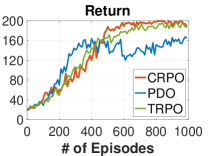
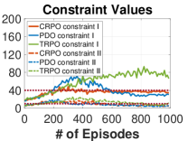
(a) Cartpole

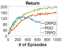
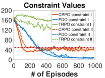
(b) Acrobot

Figure 1: Average performance for CRPO, PDO, and unconstrained TRPO over 10 seeds. The red dot lines in (a) and (b) represent the limits of the constraints.

In both tasks, CRPO tracks the constraint returns almost exactly to the limit, indicating that CRPO sufficiently explores the boundary of the feasible set, which results in an optimal return reward. In contrast, although PDO also outputs a constraints-satisfying policy in the end, it tends to over- or under-enforce the constraints, which results in lower return reward and unstable constraint satisfaction performance. In terms of the convergence, the constraints of CRPO drop below the thresholds (and thus satisfy the constraints) much faster than that of PDO, corroborating our theoretical comparison that the constraint violation of CRPO (given in Theorem 2) converges much faster than that of PDO given in (Ding et al., 2020b).

6 Conclusion

In this paper, we propose a novel CRPO approach for policy optimization for SRL, which is easy to implement and has provable global optimality guarantee. We show that CRPO achieves an $\mathcal{O}(1/\sqrt{T})$ convergence rate to the global optimum and an $\mathcal{O}(1/\sqrt{T})$ rate of vanishing constraint error when NPG update is adopted as the optimizer. This is the first primal SRL algorithm that has a provable convergence guarantee to a global optimum. In the future, it is interesting to incorporate various momentum schemes to CRPO to improve its convergence performance.

Supplementary Materials

Appendix A Experimental Setting

In our constrained Cartpole environment, the cart is restricted in the area $[-2.4,2.4]$. Each episode length is no longer than 200 and terminated when the angle of the pole is larger than 12 degree. During the training, the agent receives a reward $+1$ for every step taken, but is penalized with cost $+1$ if (1) entering the area $[-2.4,-2.2]$, $[-1.3,-1.1]$, $[-0.1,0.1]$, $[1.1,1.3]$, and $[2.2,2.4]$; or (2) having the angle of pole larger than 6 degree.

In our constrained Acrobot environment, each episode has length 500. During the training, the agent receives a reward $+1$ when the end-effector is at a height of 0.5, but is penalized with cost $+1$ when (1) a torque with value $+1$ is applied when the first pendulum swings along an anticlockwise direction; or (2) a torque with value $+1$ is applied when the second pendulum swings along an anticlockwise direction with respect to the first pendulum.

For details about the update of PD, please refer to (Achiam et al., 2017)[Section 10.3.3]. The performance of PD is very sensitive to the stepsize of the dual variable’s update. If the stepsize is too small, then the dual variable will not update quickly to enforce the constraints. If the stepsize is too large, then the algorithm will behave conservatively and have low return reward. To appropriately select the stepsize for the dual variable, we conduct the experiments with the learning rates $\{0.0001,0.0005,0.001,0.005,0.01,0.05\}$ for both tasks. The learning rate $0.005$ performs the best in the first task, and the learning rate $0.0005$ performs the best in the second task. Thus, our reported result of Cartpole is with the stepsize $0.005$ and our reported result of Acrobot is with the stepsize $0.0005$.

Next, we investigate the robustness of CRPO with respect to the tolerance parameter $\eta$. We conduct the experiments under the following values of $\eta$ $\{10,5,2,1,0.5\}$ for the Acrobot environment. It can be seen from Figure 2 that the learning curves of CRPO with the tolerance parameter $\eta$ taking different values are almost the same, which indicates that the convergence performance of CRPO is robust to the value of $\eta$ over a wide range. Thus, the tolerance parameter $\eta$ does not cause much parameter tuning cost for CRPO.

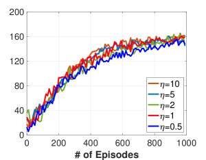
(a) Return Reward

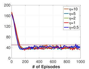
(b) Constraint Value I

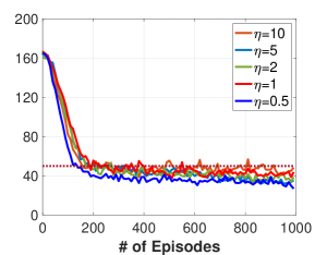
(c) Constraint Value II

Figure 2: Comparison of CRPO in Acrobot with tolerance parameter $\eta$ taking different values.

Appendix B Proof of Theorem 1: Tabular Setting

B.1 Supporting Lemmas for Poof of Theorem 1

The following lemma characterizes the convergence rate of TD learning in the tabular setting.

Lemma 2 ((Dalal et al., 2019)).

Consider the iteration given in eq. 4 with arbitrary initialization $\theta^{i}_{0}$. Assume that the stationary distribution $\mu_{\pi_{w}}$ is not degenerate for all $w\in{\mathbb{R}}^{\left|\mathcal{S}\right|\times\left|\mathcal{A}\right|}$. Let stepsize $\beta_{k}=\Theta(\frac{1}{t^{\sigma}})\,(0<\sigma<1)$. Then, with probability at least $1-\delta$, we have

$$\left\|\theta^{i}_{K}-\theta^{i}_{*}(\pi_{w})\right\|_{2}=\mathcal{O}\left(\frac{\log(\left|\mathcal{S}\right|^{2}\left|\mathcal{A}\right|^{2}K^{2}/\delta)}{(1-\gamma)K^{\sigma/2}}\right).$$

Note that $\sigma$ can be arbitrarily close to $1$. Lemma 2 implies that we can obtain an approximation $\bar{Q}^{i}_{t}$ such that $\left\|\bar{Q}^{i}_{t}-Q^{i}_{\pi_{w}}\right\|_{2}=\mathcal{O}(1/\sqrt{K_{\text{in}}})$ with high probability.

Lemma 3 (Performance difference lemma (Kakade & Langford, 2002) ).

For all policies $\pi$, $\pi^{\prime}$ and initial distribution $\rho$, we have

$$J_{i}^{\rho}(\pi)-J^{\rho}_{i}(\pi^{\prime})=\frac{1}{1-\gamma}{\mathbb{E}}_{s\sim\nu_{\rho}}{\mathbb{E}}_{a\sim\pi(\cdot|s)}[A^{i}_{\pi^{\prime}}(s,a)]$$

where $J^{\rho}_{i}(\pi)$ and $\nu_{\rho}$ denote the accumulated reward (cost) function and visitation distribution under policy $\pi$ when the initial state distribution is $\rho$.

Lemma 4 (Lemma 5.6. (Agarwal et al., 2019)).

Considering the approximated NPG update in line 7 of Algorithm 1 in the tabular setting and $i=0$, the NPG update takes the form:

$$w_{t+1}=w_{t}+\frac{\alpha}{1-\gamma}\bar{Q}^{i}_{t},\quad\text{and}\quad\pi_{w_{t+1}}(a|s)=\pi_{w_{t}}(a|s)\frac{\exp(\alpha\bar{Q}^{i}_{t}(s,a)/(1-\gamma))}{Z_{t}(s)},$$

where

$$Z_{t}(s)=\sum_{a\in\mathcal{A}}\pi_{w_{t}}(a|s)\exp\left(\frac{\alpha\bar{Q}^{i}_{t}(s,a)}{1-\gamma}\right).$$

Note that if we follow the update in line 10 of Algorithm 1, we can obtain similar results for the case $i\in\{1,\cdots,p\}$ as stated in Lemma 4.

Lemma 5 (Policy gradient property of softmax parameterization).

Considering the softmax policy in the tabular setting (eq. 3). For any initial state distribution $\rho$, we have

$$\nabla_{w}J^{\rho}_{i}(w)={\mathbb{E}}_{s\sim\nu_{\rho}}{\mathbb{E}}_{a\sim\pi_{w}(\cdot|s)}\left[\left(\mathds{1}_{as}-\sum_{a^{\prime}\in\mathcal{A}}\pi_{w}(a^{\prime}|s)\mathds{1}_{a^{\prime}s}\right)Q^{i}_{\pi_{w}}(s,a)\right],$$

and

$$\left\|\nabla_{w}J^{\rho}_{i}(w)\right\|_{2}\leq\frac{2c_{\max}}{1-\gamma},$$

where $\mathds{1}_{as}$ is an $\left|\mathcal{S}\right|\times\left|\mathcal{A}\right|$-dimension vector, with $(a,s)$-th element being one, and the rest elements being zero.

Proof.

The first result can follows directly from Lemma C.1 in (Agarwal et al., 2019). We now proceed to prove the second result.

$$\left\|\nabla_{w}J^{\rho}_{i}(w)\right\|_{2} =\left\|{\mathbb{E}}\left[\left(\mathds{1}_{as}-\sum_{a^{\prime}\in\mathcal{A}}\pi_{w}(a^{\prime}|s)\mathds{1}_{a^{\prime}s}\right)Q^{i}_{\pi_{w}}(s,a)\right]\right\|_{2}$$

$$\leq{\mathbb{E}}\left[\left\|\left(\mathds{1}_{as}-\sum_{a^{\prime}\in\mathcal{A}}\pi_{w}(a^{\prime}|s)\mathds{1}_{a^{\prime}s}\right)Q^{i}_{\pi_{w}}(s,a)\right\|_{2}\right]$$

$$\leq{\mathbb{E}}\left[\left\|\mathds{1}_{as}-\sum_{a^{\prime}\in\mathcal{A}}\pi_{w}(a^{\prime}|s)\mathds{1}_{a^{\prime}s}\right\|_{2}Q^{i}_{\pi_{w}}(s,a)\right]$$

$$\leq 2{\mathbb{E}}\left[Q^{i}_{\pi_{w}}(s,a)\right]\leq\frac{2c_{\max}}{1-\gamma}.$$

∎

Lemma 6 (Performance improvement bound for approximated NPG).

For the iterates $\pi_{w_{t}}$ generated by the approximated NPG updates in line 7 of Algorithm 1 in the tabular setting, we have for all initial state distribution $\rho$ and when $i=0$, the following holds

$$J^{\rho}_{0}(w_{t+1})-J^{\rho}_{0}(w_{t})$$

$$\geq\frac{1-\gamma}{\alpha}{\mathbb{E}}_{s\sim\rho}\left(\log Z_{t}(s)-\frac{\alpha}{1-\gamma}V^{0}_{\pi_{w_{t}}}(s)+\frac{\alpha}{1-\gamma}\sum_{a\in\mathcal{A}}\pi_{w_{t}}(a|s)\left|\bar{Q}^{0}_{t}(s,a)-Q^{0}_{\pi_{w_{t}}}(s,a)\right|\right)$$

$$\quad-\frac{1}{1-\gamma}{\mathbb{E}}_{s\sim\nu_{\rho}}\sum_{a\in\mathcal{A}}\pi_{w_{t}}(a|s)\left|\bar{Q}^{0}_{t}(s,a)-Q^{0}_{\pi_{w_{t}}}(s,a)\right|$$

$$\quad-\frac{1}{1-\gamma}{\mathbb{E}}_{s\sim\nu_{\rho}}\sum_{a\in\mathcal{A}}\pi_{w_{t+1}}(a|s)\left|Q^{0}_{\pi_{w_{t}}}(s,a)-\bar{Q}^{0}_{t}(s,a)\right|.$$

Proof.

We first provide the following lower bound.

$$\log Z_{t}(s)-\frac{\alpha}{1-\gamma}V^{i}_{\pi_{w_{t}}}(s)$$

$$=\log\sum_{a\in\mathcal{A}}\pi_{w_{t}}(a|s)\exp\left(\frac{\alpha\bar{Q}^{i}_{t}(s,a)}{1-\gamma}\right)-\frac{\alpha}{1-\gamma}V^{i}_{\pi_{w_{t}}}(s)$$

$$\geq\sum_{a\in\mathcal{A}}\pi_{w_{t}}(a|s)\log\exp\left(\frac{\alpha\bar{Q}^{i}_{t}(s,a)}{1-\gamma}\right)-\frac{\alpha}{1-\gamma}V^{i}_{\pi_{w_{t}}}(s)$$

$$=\frac{\alpha}{1-\gamma}\sum_{a\in\mathcal{A}}\pi_{w_{t}}(a|s)(\bar{Q}^{i}_{t}(s,a)-Q^{i}_{\pi_{w_{t}}}(s,a))+\frac{\alpha}{1-\gamma}\sum_{a\in\mathcal{A}}\pi_{w_{t}}(a|s)Q^{i}_{\pi_{w_{t}}}(s,a)-\frac{\alpha}{1-\gamma}V^{i}_{\pi_{w_{t}}}(s)$$

$$=\frac{\alpha}{1-\gamma}\sum_{a\in\mathcal{A}}\pi_{w_{t}}(a|s)(\bar{Q}^{i}_{t}(s,a)-Q^{i}_{\pi_{w_{t}}}(s,a))$$

$$\geq\frac{-\alpha}{1-\gamma}\sum_{a\in\mathcal{A}}\pi_{w_{t}}(a|s)\left|\bar{Q}^{i}_{t}(s,a)-Q^{i}_{\pi_{w_{t}}}(s,a)\right|.$$

Thus, we conclude that

$$\log Z_{t}(s)-\frac{\alpha}{1-\gamma}V^{i}_{\pi_{w_{t}}}(s)+\frac{\alpha}{1-\gamma}\sum_{a\in\mathcal{A}}\pi_{w_{t}}(a|s)\left|\bar{Q}^{i}_{t}(s,a)-Q^{i}_{\pi_{w_{t}}}(s,a)\right|\geq 0.$$

We then proceed to prove Lemma 6. The performance difference lemma (Lemma 3) implies:

$$J^{\rho}_{i}(w_{t+1})-J^{\rho}_{i}(w_{t})$$

$$=\frac{1}{1-\gamma}{\mathbb{E}}_{s\sim\nu_{\rho}}\sum_{a\in\mathcal{A}}\pi_{w_{t+1}}(a|s)A^{i}_{\pi_{w_{t}}}(s,a)$$

$$=\frac{1}{1-\gamma}{\mathbb{E}}_{s\sim\nu_{\rho}}\sum_{a\in\mathcal{A}}\pi_{w_{t+1}}(a|s)Q^{i}_{\pi_{w_{t}}}(s,a)-\frac{1}{1-\gamma}{\mathbb{E}}_{s\sim\nu_{\rho}}V^{i}_{\pi_{w_{t}}}(s)$$

$$=\frac{1}{1-\gamma}{\mathbb{E}}_{s\sim\nu_{\rho}}\sum_{a\in\mathcal{A}}\pi_{w_{t+1}}(a|s)\bar{Q}^{i}_{t}(s,a)+\frac{1}{1-\gamma}{\mathbb{E}}_{s\sim\nu_{\rho}}\sum_{a\in\mathcal{A}}\pi_{w_{t+1}}(a|s)(Q^{i}_{\pi_{w_{t}}}(s,a)-\bar{Q}^{i}_{t}(s,a))$$

$$\quad-\frac{1}{1-\gamma}{\mathbb{E}}_{s\sim\nu_{\rho}}V^{i}_{\pi_{w_{t}}}(s)$$

$$\overset{(i)}{=}\frac{1}{\alpha}{\mathbb{E}}_{s\sim\nu_{\rho}}\sum_{a\in\mathcal{A}}\pi_{w_{t+1}}(a|s)\log\left(\frac{\pi_{w_{t+1}}(a|s)Z_{t}(s)}{\pi_{w_{t}}(a|s)}\right)$$

$$\quad+\frac{1}{1-\gamma}{\mathbb{E}}_{s\sim\nu_{\rho}}\sum_{a\in\mathcal{A}}\pi_{w_{t+1}}(a|s)(Q^{i}_{\pi_{w_{t}}}(s,a)-\bar{Q}^{i}_{t}(s,a))-\frac{1}{1-\gamma}{\mathbb{E}}_{s\sim\nu_{\rho}}V^{i}_{\pi_{w_{t}}}(s)$$

$$=\frac{1}{\alpha}{\mathbb{E}}_{s\sim\nu_{\rho}}D_{\text{KL}}(\pi_{w_{t+1}}||\pi_{w_{t}})+\frac{1}{\alpha}{\mathbb{E}}_{s\sim\nu_{\rho}}\log Z_{t}(s)$$

$$\quad+\frac{1}{1-\gamma}{\mathbb{E}}_{s\sim\nu_{\rho}}\sum_{a\in\mathcal{A}}\pi_{w_{t+1}}(a|s)(Q^{i}_{\pi_{w_{t}}}(s,a)-\bar{Q}^{i}_{t}(s,a))-\frac{1}{1-\gamma}{\mathbb{E}}_{s\sim\nu_{\rho}}V^{i}_{\pi_{w_{t}}}(s)$$

$$\geq\frac{1}{\alpha}{\mathbb{E}}_{s\sim\nu_{\rho}}\left(\log Z_{t}(s)-\frac{\alpha}{1-\gamma}V^{i}_{\pi_{w_{t}}}(s)+\frac{\alpha}{1-\gamma}\sum_{a\in\mathcal{A}}\pi_{w_{t}}(a|s)\left|\bar{Q}^{i}_{t}(s,a)-Q^{i}_{\pi_{w_{t}}}(s,a)\right|\right)$$

$$\quad-\frac{1}{1-\gamma}{\mathbb{E}}_{s\sim\nu_{\rho}}\sum_{a\in\mathcal{A}}\pi_{w_{t}}(a|s)\left|\bar{Q}^{i}_{t}(s,a)-Q^{i}_{\pi_{w_{t}}}(s,a)\right|$$

$$\quad-\frac{1}{1-\gamma}{\mathbb{E}}_{s\sim\nu_{\rho}}\sum_{a\in\mathcal{A}}\pi_{w_{t+1}}(a|s)\left|Q^{i}_{\pi_{w_{t}}}(s,a)-\bar{Q}^{i}_{t}(s,a)\right|$$

$$\overset{(ii)}{\geq}\frac{1-\gamma}{\alpha}{\mathbb{E}}_{s\sim\rho}\left(\log Z_{t}(s)-\frac{\alpha}{1-\gamma}V^{i}_{\pi_{w_{t}}}(s)+\frac{\alpha}{1-\gamma}\sum_{a\in\mathcal{A}}\pi_{w_{t}}(a|s)\left|\bar{Q}^{i}_{t}(s,a)-Q^{i}_{\pi_{w_{t}}}(s,a)\right|\right)$$

$$\quad-\frac{1}{1-\gamma}{\mathbb{E}}_{s\sim\nu_{\rho}}\sum_{a\in\mathcal{A}}\pi_{w_{t}}(a|s)\left|\bar{Q}^{i}_{t}(s,a)-Q^{i}_{\pi_{w_{t}}}(s,a)\right|$$

$$\quad-\frac{1}{1-\gamma}{\mathbb{E}}_{s\sim\nu_{\rho}}\sum_{a\in\mathcal{A}}\pi_{w_{t+1}}(a|s)\left|Q^{i}_{\pi_{w_{t}}}(s,a)-\bar{Q}^{i}_{t}(s,a)\right|$$

where $(i)$ follows from the update rule in Lemma 4 and $(ii)$ follows from the facts that $\left\|\nu_{\rho}/\rho\right\|_{\infty}\geq 1-\gamma$ and $\log Z_{t}(s)-\frac{\alpha}{1-\gamma}V^{i}_{\pi_{w_{t}}}(s)+\frac{\alpha}{1-\gamma}\sum_{a\in\mathcal{A}}\pi_{w_{t}}(a|s)\left|\bar{Q}^{i}_{t}(s,a)-Q^{i}_{\pi_{w_{t}}}(s,a)\right|\geq 0$. ∎

Note that if we follow the update in line 10 of Algorithm 1, we can obtain similar results for the case $i\in\{1,\cdots,p\}$ as stated in Lemma 6.

Lemma 7 (Upper bound on optimality gap for approximated NPG).

Consider the approximated NPG updates in line 7 of Algorithm 1 in the tabular setting when $i=0$. We have

$$J_{0}(\pi^{*})-J_{0}(\pi_{w_{t}})$$

$$\leq\frac{1}{\alpha}{\mathbb{E}}_{s\sim\nu^{*}}(D_{\text{KL}}(\pi^{*}||\pi_{w_{t}})-D_{\text{KL}}(\pi^{*}||\pi_{w_{t+1}}))+\frac{2\alpha c^{2}_{\max}\left|\mathcal{S}\right|\left|\mathcal{A}\right|}{(1-\gamma)^{3}}+\frac{3(1+\alpha c_{\max})}{(1-\gamma)^{2}}\left\|Q^{0}_{\pi_{w_{t}}}-\bar{Q}^{0}_{t}\right\|_{2}.$$

Proof.

By the performance difference lemma (Lemma 3), we have

$$J_{i}(\pi^{*})-J_{i}(\pi_{w_{t}})$$

$$=\frac{1}{1-\gamma}{\mathbb{E}}_{s\sim\nu^{*}}\sum_{a\in\mathcal{A}}\pi^{*}(a|s)A^{i}_{\pi_{w_{t}}}(s,a)$$

$$=\frac{1}{1-\gamma}{\mathbb{E}}_{s\sim\nu^{*}}\sum_{a\in\mathcal{A}}\pi^{*}(a|s)Q^{i}_{\pi_{w_{t}}}(s,a)-\frac{1}{1-\gamma}{\mathbb{E}}_{s\sim\nu^{*}}V^{i}_{\pi_{w_{t}}}(s)$$

$$=\frac{1}{1-\gamma}{\mathbb{E}}_{s\sim\nu^{*}}\sum_{a\in\mathcal{A}}\pi^{*}(a|s)\bar{Q}^{i}_{t}(s,a)+\frac{1}{1-\gamma}{\mathbb{E}}_{s\sim\nu^{*}}\sum_{a\in\mathcal{A}}\pi^{*}(a|s)(Q^{i}_{\pi_{w_{t}}}(s,a)-\bar{Q}^{i}_{t}(s,a))$$

$$\quad-\frac{1}{1-\gamma}{\mathbb{E}}_{s\sim\nu^{*}}V^{i}_{\pi_{w_{t}}}(s)$$

$$\overset{(i)}{=}\frac{1}{1-\gamma}{\mathbb{E}}_{s\sim\nu^{*}}\sum_{a\in\mathcal{A}}\pi^{*}(a|s)\log\frac{\pi_{w_{t+1}}(a|s)Z_{t}(s)}{\pi_{w_{t}}(a|s)}+\frac{1}{1-\gamma}{\mathbb{E}}_{s\sim\nu^{*}}\sum_{a\in\mathcal{A}}\pi^{*}(a|s)(Q^{i}_{\pi_{w_{t}}}(s,a)-\bar{Q}^{i}_{t}(s,a))$$

$$\quad-\frac{1}{1-\gamma}{\mathbb{E}}_{s\sim\nu^{*}}V^{i}_{\pi_{w_{t}}}(s)$$

$$=\frac{1}{\alpha}{\mathbb{E}}_{s\sim\nu^{*}}(D_{\text{KL}}(\pi^{*}||\pi_{w_{t}})-D_{\text{KL}}(\pi^{*}||\pi_{w_{t+1}}))+\frac{1}{\alpha}{\mathbb{E}}_{s\sim\nu^{*}}\left(\log Z_{t}(s)-\frac{\alpha}{1-\gamma}V^{i}_{\pi_{w_{t}}}(s)\right)$$

$$\quad+\frac{1}{1-\gamma}{\mathbb{E}}_{s\sim\nu^{*}}\sum_{a\in\mathcal{A}}\pi^{*}(a|s)(Q^{i}_{\pi_{w_{t}}}(s,a)-\bar{Q}^{i}_{t}(s,a))$$

$$\leq\frac{1}{\alpha}{\mathbb{E}}_{s\sim\nu^{*}}(D_{\text{KL}}(\pi^{*}||\pi_{w_{t}})-D_{\text{KL}}(\pi^{*}||\pi_{w_{t+1}}))$$

$$\quad+\frac{1}{\alpha}{\mathbb{E}}_{s\sim\nu^{*}}\left(\log Z_{t}(s)-\frac{\alpha}{1-\gamma}V^{i}_{\pi_{w_{t}}}(s)+\frac{\alpha}{1-\gamma}\sum_{a\in\mathcal{A}}\pi_{w_{t}}(a|s)\left|\bar{Q}^{i}_{t}(s,a)-Q^{i}_{\pi_{w_{t}}}(s,a)\right|\right)$$

$$\quad+\frac{1}{1-\gamma}{\mathbb{E}}_{s\sim\nu^{*}}\sum_{a\in\mathcal{A}}\pi^{*}(a|s)(Q^{i}_{\pi_{w_{t}}}(s,a)-\bar{Q}^{i}_{t}(s,a))$$

$$\overset{(ii)}{\leq}\frac{1}{\alpha}{\mathbb{E}}_{s\sim\nu^{*}}(D_{\text{KL}}(\pi^{*}||\pi_{w_{t}})-D_{\text{KL}}(\pi^{*}||\pi_{w_{t+1}}))$$

$$\quad+\frac{1}{1-\gamma}(J^{\nu^{*}}_{i}(w_{t+1})-J^{\nu^{*}}_{i}(w_{t}))+\frac{1}{(1-\gamma)^{2}}{\mathbb{E}}_{s\sim\nu_{\nu^{*}}}\sum_{a\in\mathcal{A}}\pi_{w_{t+1}}(a|s)\left|Q^{i}_{\pi_{w_{t}}}(s,a)-\bar{Q}^{i}_{t}(s,a)\right|$$

$$\quad+\frac{1}{(1-\gamma)^{2}}{\mathbb{E}}_{s\sim\nu_{\nu^{*}}}\sum_{a\in\mathcal{A}}\pi_{w_{t}}(a|s)\left|Q^{i}_{\pi_{w_{t}}}(s,a)-\bar{Q}^{i}_{t}(s,a)\right|$$

$$\quad+\frac{1}{1-\gamma}{\mathbb{E}}_{s\sim\nu^{*}}\sum_{a\in\mathcal{A}}\pi^{*}(a|s)\left|Q^{i}_{\pi_{w_{t}}}(s,a)-\bar{Q}^{i}_{t}(s,a)\right|$$

$$\overset{(iii)}{\leq}\frac{1}{\alpha}{\mathbb{E}}_{s\sim\nu^{*}}(D_{\text{KL}}(\pi^{*}||\pi_{w_{t}})-D_{\text{KL}}(\pi^{*}||\pi_{w_{t+1}}))+\frac{2c_{\max}}{(1-\gamma)^{2}}\left\|w_{t+1}-w_{t}\right\|_{2}+\frac{3}{(1-\gamma)^{2}}\left\|Q^{i}_{\pi_{w_{t}}}-\bar{Q}^{i}_{t}\right\|_{2}$$

$$=\frac{1}{\alpha}{\mathbb{E}}_{s\sim\nu^{*}}(D_{\text{KL}}(\pi^{*}||\pi_{w_{t}})-D_{\text{KL}}(\pi^{*}||\pi_{w_{t+1}}))+\frac{2\alpha c_{\max}}{(1-\gamma)^{2}}\left\|\bar{Q}^{i}_{t}\right\|_{2}+\frac{3}{(1-\gamma)^{2}}\left\|Q^{i}_{\pi_{w_{t}}}-\bar{Q}^{i}_{t}\right\|_{2}$$

$$\leq\frac{1}{\alpha}{\mathbb{E}}_{s\sim\nu^{*}}(D_{\text{KL}}(\pi^{*}||\pi_{w_{t}})-D_{\text{KL}}(\pi^{*}||\pi_{w_{t+1}}))+\frac{2\alpha c_{\max}}{(1-\gamma)^{2}}\left\|Q^{i}_{\pi_{w_{t}}}\right\|_{2}+\frac{3(1+\alpha c_{\max})}{(1-\gamma)^{2}}\left\|Q^{i}_{\pi_{w_{t}}}-\bar{Q}^{i}_{t}\right\|_{2}$$

$$\leq\frac{1}{\alpha}{\mathbb{E}}_{s\sim\nu^{*}}(D_{\text{KL}}(\pi^{*}||\pi_{w_{t}})-D_{\text{KL}}(\pi^{*}||\pi_{w_{t+1}}))+\frac{2\alpha c^{2}_{\max}\left|\mathcal{S}\right|\left|\mathcal{A}\right|}{(1-\gamma)^{3}}+\frac{3(1+\alpha c_{\max})}{(1-\gamma)^{2}}\left\|Q^{i}_{\pi_{w_{t}}}-\bar{Q}^{i}_{t}\right\|_{2},$$

where $(i)$ follows from Lemma 4, $(ii)$ follows from Lemma 6 and $(iii)$ follows from the Lipschitz property of $J^{\nu^{*}}_{i}(w)$ such that $J^{\nu^{*}}_{i}(w_{t+1})-J^{\nu^{*}}_{i}(w_{t})\leq\frac{2c_{\max}}{1-\gamma}\left\|w_{t+1}-w_{t}\right\|_{2}$, which is proved by Proposition 1 in (Xu et al., 2020b). ∎

Note that if we follow the update in line 10 of Algorithm 1, we can obtain the following result for the case $i\in\{1,\cdots,p\}$ as stated in Lemma 7:

$$J_{i}(\pi_{w_{t}})-J_{i}(\pi^{*})$$

$$\leq\frac{1}{\alpha}{\mathbb{E}}_{s\sim\nu^{*}}(D_{\text{KL}}(\pi^{*}||\pi_{w_{t}})-D_{\text{KL}}(\pi^{*}||\pi_{w_{t+1}}))+\frac{2\alpha c^{2}_{\max}\left|\mathcal{S}\right|\left|\mathcal{A}\right|}{(1-\gamma)^{3}}+\frac{3(1+\alpha c_{\max})}{(1-\gamma)^{2}}\left\|Q^{i}_{\pi_{w_{t}}}-\bar{Q}^{i}_{t}\right\|_{2}.$$

Lemma 8.

Considering CRPO in Algorithm 1 in the tabular setting. Let $K_{\text{in}}=\Theta(T^{1/\sigma}\log^{2/\sigma}(\left|\mathcal{S}\right|^{2}\left|\mathcal{A}\right|^{2}T^{1+2/\sigma}/\delta))$. Define ${\mathcal{N}}_{i}$ as the set of steps that CRPO algorithm chooses to minimize the $i$-th constraint. With probability at least $1-\delta$, we have

$$\sum_{t\in{\mathcal{N}}_{0}}(J_{0}(\pi^{*})-J_{0}(\pi_{w_{t}}))+\alpha\eta\sum_{i=1}^{p}\left|{\mathcal{N}}_{i}\right|$$

$$\leq{\mathbb{E}}_{s\sim\nu^{*}}D_{\text{KL}}(\pi^{*}||\pi_{w_{0}})+\frac{2\alpha^{2}c^{2}_{\max}\left|\mathcal{S}\right|\left|\mathcal{A}\right|T}{(1-\gamma)^{3}}+\frac{\alpha\sqrt{T}(2+(1-\gamma)^{2}+2\alpha c_{\max})}{(1-\gamma)^{2}}.$$

Proof.

If $t\in{\mathcal{N}}_{0}$, by Lemma 7 we have

$$\alpha(J_{0}(\pi^{*})-J_{0}(\pi_{w_{t}}))$$

$$\leq{\mathbb{E}}_{s\sim\nu^{*}}(D_{\text{KL}}(\pi^{*}||\pi_{w_{t}})-D_{\text{KL}}(\pi^{*}||\pi_{w_{t+1}}))+\frac{2\alpha^{2}c^{2}_{\max}\left|\mathcal{S}\right|\left|\mathcal{A}\right|}{(1-\gamma)^{3}}+\frac{3\alpha(1+\alpha c_{\max})}{(1-\gamma)^{2}}\left\|Q^{0}_{\pi_{w_{t}}}-\bar{Q}^{0}_{t}\right\|_{2}.$$ (12)

If $t\in{\mathcal{N}}_{i}$, similarly we can obtain

$$\alpha(J_{i}(\pi_{w_{t}})-J_{i}(\pi^{*}))$$

$$\leq{\mathbb{E}}_{s\sim\nu^{*}}(D_{\text{KL}}(\pi^{*}||\pi_{w_{t}})-D_{\text{KL}}(\pi^{*}||\pi_{w_{t+1}}))+\frac{2\alpha^{2}c^{2}_{\max}\left|\mathcal{S}\right|\left|\mathcal{A}\right|}{(1-\gamma)^{3}}+\frac{3\alpha(1+\alpha c_{\max})}{(1-\gamma)^{2}}\left\|Q^{i}_{\pi_{w_{t}}}-\bar{Q}^{i}_{t}\right\|_{2}.$$ (13)

Taking the summation of eq. 12 and eq. 13 from $t=0$ to $T-1$ yields

$$\alpha\sum_{t\in{\mathcal{N}}_{0}}(J_{0}(\pi^{*})-J_{0}(\pi_{w_{t}}))+\alpha\sum_{i=1}^{p}\sum_{t\in{\mathcal{N}}_{i}}(J_{i}(\pi_{w_{t}})-J_{i}(\pi^{*}))$$

$$\leq{\mathbb{E}}_{s\sim\nu^{*}}D_{\text{KL}}(\pi^{*}||\pi_{w_{0}})+\frac{2\alpha^{2}c^{2}_{\max}\left|\mathcal{S}\right|\left|\mathcal{A}\right|T}{(1-\gamma)^{3}}+\frac{3\alpha(1+\alpha c_{\max})}{(1-\gamma)^{2}}\sum_{i=0}^{p}\sum_{t\in{\mathcal{N}}_{i}}\left\|Q^{i}_{\pi_{w_{t}}}-\bar{Q}^{i}_{t}\right\|_{2}.$$ (14)

Note that when $t\in{\mathcal{N}}_{i}$ ($i\neq 0$), we have $\bar{J}_{i}(\theta^{i}_{t})>d_{i}+\eta$ (line 9 in Algorithm 1), which implies that

$$J_{i}(\pi_{w_{t}})-J_{i}(\pi^{*}) \geq\bar{J}_{i}(\theta^{i}_{t})-J_{i}(\pi^{*})-\left|\bar{J}_{i}(\theta^{i}_{t})-J_{i}(\pi_{w_{t}})\right|$$

$$\geq d_{i}+\eta-J_{i}(\pi^{*})-\left|\bar{J}_{i}(\theta^{i}_{t})-J_{i}(\pi_{w_{t}})\right|$$

$$\geq\eta-\left\|Q^{i}_{\pi_{w}}-\bar{Q}^{i}_{t}\right\|_{2}.$$ (15)

Substituting eq. 15 into eq. 14 yields

$$\alpha\sum_{t\in{\mathcal{N}}_{0}}(J_{0}(\pi^{*})-J_{0}(\pi_{w_{t}}))+\alpha\eta\sum_{i=1}^{p}\left|{\mathcal{N}}_{i}\right|-\alpha\sum_{i=1}^{p}\sum_{t\in{\mathcal{N}}_{i}}\left\|Q^{i}_{\pi_{w_{t}}}-\bar{Q}^{i}_{t}\right\|_{2}$$

$$\leq{\mathbb{E}}_{s\sim\nu^{*}}D_{\text{KL}}(\pi^{*}||\pi_{w_{0}})+\frac{2\alpha^{2}c^{2}_{\max}\left|\mathcal{S}\right|\left|\mathcal{A}\right|T}{(1-\gamma)^{3}}+\frac{3\alpha(1+\alpha c_{\max})}{(1-\gamma)^{2}}\sum_{i=0}^{p}\sum_{t\in{\mathcal{N}}_{i}}\left\|Q^{i}_{\pi_{w_{t}}}-\bar{Q}^{i}_{t}\right\|_{2},$$

which implies

$$\alpha\sum_{t\in{\mathcal{N}}_{0}}(J_{0}(\pi^{*})-J_{0}(\pi_{w_{t}}))+\alpha\eta\sum_{i=1}^{p}\left|{\mathcal{N}}_{i}\right|$$

$$\leq{\mathbb{E}}_{s\sim\nu^{*}}D_{\text{KL}}(\pi^{*}||\pi_{w_{0}})+\frac{2\alpha^{2}c^{2}_{\max}\left|\mathcal{S}\right|\left|\mathcal{A}\right|T}{(1-\gamma)^{3}}+\frac{\alpha(2+(1-\gamma)^{2}+3\alpha c_{\max})}{(1-\gamma)^{2}}\sum_{i=0}^{p}\sum_{t\in{\mathcal{N}}_{i}}\left\|Q^{i}_{\pi_{w_{t}}}-\bar{Q}^{i}_{t}\right\|_{2}.$$ (16)

By Lemma 2, we have with probability at least $1-\delta$, the following holds

$$\left\|Q^{i}_{\pi_{w_{t}}}-\bar{Q}^{i}_{t}\right\|_{2}=\mathcal{O}\left(\frac{\log(\left|\mathcal{S}\right|^{2}\left|\mathcal{A}\right|^{2}K_{\text{in}}^{2}/\delta)}{(1-\gamma)K_{\text{in}}^{\sigma/2}}\right).$$

Thus, if we let

$$K_{\text{in}}=\Theta\left(\left(\frac{T}{(1-\gamma)^{2}\left|\mathcal{S}\right|\left|\mathcal{A}\right|}\right)^{\frac{1}{\sigma}}\log^{\frac{2}{\sigma}}\left(\frac{T^{\frac{2}{\sigma}+1}}{\delta(1-\gamma)^{\frac{2}{\sigma}}\left|\mathcal{S}\right|^{\frac{2}{\sigma}-2}\left|\mathcal{A}\right|^{\frac{2}{\sigma}-2}}\right)\right),$$

then with probability at least $1-\delta/T$, we have

$$\left\|Q^{i}_{\pi_{w_{t}}}-\bar{Q}^{i}_{t}\right\|_{2}\leq\frac{\sqrt{(1-\gamma)\left|\mathcal{S}\right|\left|\mathcal{A}\right|}}{\sqrt{T}}.$$ (17)

Applying the union bound to eq. 17 from $t=0$ to $T-1$, we have with probability at least $1-\delta$ the following holds

$$\sum_{i=0}^{p}\sum_{t\in{\mathcal{N}}_{i}}\left\|Q^{i}_{\pi_{w_{t}}}-\bar{Q}^{i}_{t}\right\|_{2}\leq\sqrt{(1-\gamma)\left|\mathcal{S}\right|\left|\mathcal{A}\right|T},$$ (18)

which further implies that, with probability at least $1-\delta$, we have

$$\alpha\sum_{t\in{\mathcal{N}}_{0}}(J_{0}(\pi^{*})-J_{0}(\pi_{w_{t}}))+\alpha\eta\sum_{i=1}^{p}\left|{\mathcal{N}}_{i}\right|$$

$$\leq{\mathbb{E}}_{s\sim\nu^{*}}D_{\text{KL}}(\pi^{*}||\pi_{w_{0}})+\frac{2\alpha^{2}c^{2}_{\max}\left|\mathcal{S}\right|\left|\mathcal{A}\right|T}{(1-\gamma)^{3}}+\frac{\alpha\sqrt{\left|\mathcal{S}\right|\left|\mathcal{A}\right|T}(2+(1-\gamma)^{2}+3\alpha c_{\max})}{(1-\gamma)^{1.5}},$$

which completes the proof. ∎

Lemma 9.

If

$$\frac{1}{2}\alpha\eta T\geq{\mathbb{E}}_{s\sim\nu^{*}}D_{\text{KL}}(\pi^{*}||\pi_{w_{0}})+\frac{2\alpha^{2}c^{2}_{\max}\left|\mathcal{S}\right|\left|\mathcal{A}\right|T}{(1-\gamma)^{3}}+\frac{\alpha\sqrt{\left|\mathcal{S}\right|\left|\mathcal{A}\right|T}(2+(1-\gamma)^{2}+3\alpha c_{\max})}{(1-\gamma)^{1.5}},$$ (19)

then with probability at least $1-\delta$, we have the following holds

1. ${\mathcal{N}}_{0}\neq\emptyset$, i.e., $w_{\text{out}}$ is well-defined,

2. One of the following two statements must hold,

   1. $\left|{\mathcal{N}}_{0}\right|\geq T/2$,

   2. $\sum_{t\in{\mathcal{G}}}(J_{0}(\pi^{*})-J_{0}(w_{t}))\leq 0$.

Proof.

We prove Lemma 9 in the event that eq. 18 holds, which happens with probability at least $1-\delta$. Under such an event, the following inequality holds, which is also the result of Lemma 8.

$$\alpha\sum_{t\in{\mathcal{N}}_{0}}(J_{0}(\pi^{*})-J_{0}(\pi_{w_{t}}))+\alpha\eta\sum_{i=1}^{p}\left|{\mathcal{N}}_{i}\right|$$

$$\leq{\mathbb{E}}_{s\sim\nu^{*}}D_{\text{KL}}(\pi^{*}||\pi_{w_{0}})+\frac{2\alpha^{2}c^{2}_{\max}\left|\mathcal{S}\right|\left|\mathcal{A}\right|T}{(1-\gamma)^{3}}+\frac{\alpha\sqrt{\left|\mathcal{S}\right|\left|\mathcal{A}\right|T}(2+(1-\gamma)^{2}+2\alpha c_{\max})}{(1-\gamma)^{1.5}}.$$ (20)

We first verify item 1. If ${\mathcal{N}}_{0}=\emptyset$, then $\sum_{i=1}^{p}\left|{\mathcal{N}}_{i}\right|=T$, and eq. 20 implies that

$$\alpha\eta T\leq{\mathbb{E}}_{s\sim\nu^{*}}D_{\text{KL}}(\pi^{*}||\pi_{w_{0}})+\frac{2\alpha^{2}c^{2}_{\max}\left|\mathcal{S}\right|\left|\mathcal{A}\right|T}{(1-\gamma)^{3}}+\frac{\alpha\sqrt{\left|\mathcal{S}\right|\left|\mathcal{A}\right|T}(2+(1-\gamma)^{2}+2\alpha c_{\max})}{(1-\gamma)^{1.5}},$$

which contradicts eq. 19. Thus, we must have ${\mathcal{N}}_{0}\neq\emptyset$.

We then proceed to verify item 2. If $\sum_{t\in{\mathcal{N}}_{0}}(J_{0}(\pi^{*})-J_{0}(w_{t}))\leq 0$, then (b) in item 2 holds. If $\sum_{t\in{\mathcal{N}}_{0}}(J_{0}(\pi^{*})-J_{0}(w_{t}))\leq 0$, then eq. 20 implies that

$$\alpha\eta\sum_{i=1}^{p}\left|{\mathcal{N}}_{i}\right|\leq{\mathbb{E}}_{s\sim\nu^{*}}D_{\text{KL}}(\pi^{*}||\pi_{w_{0}})+\frac{2\alpha^{2}c^{2}_{\max}\left|\mathcal{S}\right|\left|\mathcal{A}\right|T}{(1-\gamma)^{3}}+\frac{\alpha\sqrt{\left|\mathcal{S}\right|\left|\mathcal{A}\right|T}(2+(1-\gamma)^{2}+3\alpha c_{\max})}{(1-\gamma)^{1.5}}.$$

Suppose that $\left|{\mathcal{N}}_{0}\right|<T/2$, i.e., $\sum_{i=1}^{p}\left|{\mathcal{N}}_{i}\right|\geq T/2$. Then,

$$\frac{1}{2}\alpha\eta T \leq\alpha\eta\sum_{i=1}^{p}\left|{\mathcal{N}}_{i}\right|$$

$$\leq{\mathbb{E}}_{s\sim\nu^{*}}D_{\text{KL}}(\pi^{*}||\pi_{w_{0}})+\frac{2\alpha^{2}c^{2}_{\max}\left|\mathcal{S}\right|\left|\mathcal{A}\right|T}{(1-\gamma)^{3}}+\frac{\alpha\sqrt{\left|\mathcal{S}\right|\left|\mathcal{A}\right|T}(2+(1-\gamma)^{2}+3\alpha c_{\max})}{(1-\gamma)^{1.5}},$$

which contradicts eq. 19. Hence, (a) in item 2 holds. ∎

B.2 Proof of Theorem 1

We restate Theorem 1 as follows to include the specifics of the parameters.

Theorem 3 (Restatement of Theorem 1).

Consider Algorithm 1 in the tabular setting. Let $\alpha=(1-\gamma)^{1.5}/\sqrt{\left|\mathcal{S}\right|\left|\mathcal{A}\right|T}$, $\eta=\frac{2\sqrt{\left|\mathcal{S}\right|\left|\mathcal{A}\right|}}{(1-\gamma)^{1.5}\sqrt{T}}(3+{\mathbb{E}}_{s\sim\nu^{*}}D_{\text{KL}}(\pi^{*}||\pi_{w_{0}})+3c_{\max}+c^{2}_{\max})$, and

$$K_{\text{in}}=\Theta\left(\left(\frac{T}{(1-\gamma)\left|\mathcal{S}\right|\left|\mathcal{A}\right|}\right)^{\frac{1}{\sigma}}\log^{\frac{2}{\sigma}}\left(\frac{T^{\frac{2}{\sigma}+1}}{\delta(1-\gamma)^{\frac{2}{\sigma}}\left|\mathcal{S}\right|^{\frac{2}{\sigma}-2}\left|\mathcal{A}\right|^{\frac{2}{\sigma}-2}}\right)\right).$$

Suppose the same setting for policy evaluation in Lemma 2 hold. Then, with probability at least $1-\delta$, we have

$$J_{0}(\pi^{*})-{\mathbb{E}}[J_{0}(w_{\text{out}})]=\frac{2\sqrt{\left|\mathcal{S}\right|\left|\mathcal{A}\right|}}{(1-\gamma)^{1.5}\sqrt{T}}\left({\mathbb{E}}_{s\sim\nu^{*}}D_{\text{KL}}(\pi^{*}||\pi_{w_{0}})+3+2c^{2}_{\max}+3c_{\max}\right),$$

and for all $i\in\{1,\cdots,p\}$, we have

$${\mathbb{E}}[J_{i}(\pi_{w_{\text{out}}})]-d_{i}\leq\frac{2\sqrt{\left|\mathcal{S}\right|\left|\mathcal{A}\right|}}{(1-\gamma)^{1.5}\sqrt{T}}(3+{\mathbb{E}}_{s\sim\nu^{*}}D_{\text{KL}}(\pi^{*}||\pi_{w_{0}})+3c_{\max}+c^{2}_{\max})+\frac{2\sqrt{(1-\gamma)\left|\mathcal{S}\right|\left|\mathcal{A}\right|}}{\sqrt{T}}.$$

To prove Theorem 1 (or Theorem 3), we still consider the following event given in eq. 18 that happens with probability at least $1-\delta$:

$$\sum_{i=0}^{p}\sum_{t\in{\mathcal{N}}_{i}}\left\|Q^{i}_{\pi_{w_{t}}}-\bar{Q}^{i}_{t}\right\|_{2}\leq\sqrt{(1-\gamma)\left|\mathcal{S}\right|\left|\mathcal{A}\right|T},$$

which implies

$$\alpha\sum_{t\in{\mathcal{N}}_{0}}(J_{0}(\pi^{*})-J_{0}(\pi_{w_{t}}))+\alpha\eta\sum_{i=1}^{p}\left|{\mathcal{N}}_{i}\right|$$

$$\leq{\mathbb{E}}_{s\sim\nu^{*}}D_{\text{KL}}(\pi^{*}||\pi_{w_{0}})+\frac{2\alpha^{2}c^{2}_{\max}\left|\mathcal{S}\right|\left|\mathcal{A}\right|T}{(1-\gamma)^{3}}+\frac{\alpha\sqrt{\left|\mathcal{S}\right|\left|\mathcal{A}\right|T}(2+(1-\gamma)^{2}+3\alpha c_{\max})}{(1-\gamma)^{1.5}}.$$

We first consider the convergence rate of the objective function. Under the above event, the following holds

$$\alpha\sum_{t\in{\mathcal{N}}_{0}}(J_{0}(\pi^{*})-J_{0}(\pi_{w_{t}}))$$

$$\leq{\mathbb{E}}_{s\sim\nu^{*}}D_{\text{KL}}(\pi^{*}||\pi_{w_{0}})+\frac{2\alpha^{2}c^{2}_{\max}\left|\mathcal{S}\right|\left|\mathcal{A}\right|T}{(1-\gamma)^{3}}+\frac{\alpha\sqrt{\left|\mathcal{S}\right|\left|\mathcal{A}\right|T}(2+(1-\gamma)^{2}+3\alpha c_{\max})}{(1-\gamma)^{1.5}}.$$

If $\sum_{t\in{\mathcal{N}}_{0}}(J_{0}(\pi^{*})-J_{0}(\pi_{w_{t}}))\leq 0$, then we have $J_{0}(\pi^{*})-J_{0}(\pi_{w_{\text{out}}})\leq 0$. If $\sum_{t\in{\mathcal{N}}_{0}}(J_{0}(\pi^{*})-J_{0}(\pi_{w_{t}}))\geq 0$, we have $\left|{\mathcal{N}}_{0}\right|\geq T/2$, which implies the following convergence rate

$$J_{0}(\pi^{*})-{\mathbb{E}}[J_{0}(\pi_{w_{\text{out}}})]$$

$$=\frac{1}{\left|{\mathcal{N}}_{0}\right|}\sum_{t\in{\mathcal{N}}_{0}}(J_{0}(\pi^{*})-J_{0}(\pi_{w_{t}}))$$

$$\leq\frac{2}{\alpha T}{\mathbb{E}}_{s\sim\nu^{*}}D_{\text{KL}}(\pi^{*}||\pi_{w_{0}})+\frac{4\alpha c^{2}_{\max}\left|\mathcal{S}\right|\left|\mathcal{A}\right|}{(1-\gamma)^{3}}+\frac{2\sqrt{\left|\mathcal{S}\right|\left|\mathcal{A}\right|}(2+(1-\gamma)^{2}+3\alpha c_{\max})}{(1-\gamma)^{1.5}\sqrt{T}}$$

$$\leq\frac{\sqrt{\left|\mathcal{S}\right|\left|\mathcal{A}\right|}}{(1-\gamma)^{1.5}\sqrt{T}}\left(2{\mathbb{E}}_{s\sim\nu^{*}}D_{\text{KL}}(\pi^{*}||\pi_{w_{0}})+6+4c^{2}_{\max}+6c_{\max}\right).$$

We then proceed to bound the constrains violation. For any $i\in\{1,\cdots,p\}$, we have

$${\mathbb{E}}[J_{i}(\pi_{w_{\text{out}}})]-d_{i} =\frac{1}{\left|{\mathcal{N}}_{0}\right|}\sum_{t\in{\mathcal{N}}_{0}}J_{i}(\pi_{w_{t}})-d_{i}$$

$$\leq\frac{1}{\left|{\mathcal{N}}_{0}\right|}\sum_{t\in{\mathcal{N}}_{0}}(\bar{J}_{i}(\theta^{i}_{t})-d_{i})+\frac{1}{\left|{\mathcal{N}}_{0}\right|}\sum_{t\in{\mathcal{N}}_{0}}\left|J_{i}(\pi_{w_{t}})-\bar{J}_{i}(\theta^{i}_{t})\right|$$

$$\leq\eta+\frac{1}{\left|{\mathcal{N}}_{0}\right|}\sum_{t=0}^{T-1}\left|J_{i}(\pi_{w_{t}})-\bar{J}_{i}(\theta^{i}_{t})\right|$$

$$\leq\eta+\frac{1}{\left|{\mathcal{N}}_{0}\right|}\sum_{i=0}^{p}\sum_{t\in{\mathcal{N}}_{i}}\left\|Q^{i}_{\pi_{w_{t}}}-\bar{Q}^{i}_{t}\right\|_{2}$$

$$\leq\eta+\frac{2}{T}\sum_{i=0}^{p}\sum_{t\in{\mathcal{N}}_{i}}\left\|Q^{i}_{\pi_{w_{t}}}-\bar{Q}^{i}_{t}\right\|_{2}.$$

Under the event defined in eq. 18, we have $\sum_{i=0}^{p}\sum_{t\in{\mathcal{N}}_{i}}\left\|Q^{i}_{\pi_{w_{t}}}-\bar{Q}^{i}_{t}\right\|_{2}\leq\sqrt{(1-\gamma)\left|\mathcal{S}\right|\left|\mathcal{A}\right|T}$. Recall the value of the tolerance $\eta=\frac{2\sqrt{\left|\mathcal{S}\right|\left|\mathcal{A}\right|}}{(1-\gamma)^{1.5}\sqrt{T}}(3+{\mathbb{E}}_{s\sim\nu^{*}}D_{\text{KL}}(\pi^{*}||\pi_{w_{0}})+3c_{\max}+c^{2}_{\max})$. With probability at least $1-\delta$, we have

$${\mathbb{E}}[J_{i}(\pi_{w_{\text{out}}})]-d_{i}\leq\frac{2\sqrt{\left|\mathcal{S}\right|\left|\mathcal{A}\right|}}{(1-\gamma)^{1.5}\sqrt{T}}(3+{\mathbb{E}}_{s\sim\nu^{*}}D_{\text{KL}}(\pi^{*}||\pi_{w_{0}})+3c_{\max}+c^{2}_{\max})+\frac{2\sqrt{(1-\gamma)\left|\mathcal{S}\right|\left|\mathcal{A}\right|}}{\sqrt{T}}.$$

Appendix C Proof of Lemma 1 and Theorem 2: Function Approximation Setting

For notation simplicity, we denote the state action pairs $(s,a)$ and $(s^{\prime},a^{\prime})$ as $x$ and $x^{\prime}$, respectively. We define the weighted norm $\left\|f\right\|_{\mathcal{D}}=\sqrt{\int f(x)^{2}d\mathcal{D}(x)}$ for any distribution $\mathcal{D}$ over $\left|\mathcal{S}\right|\times\left|\mathcal{A}\right|$. We will write $\theta^{i}_{k}$ as $\theta_{k}$ whenever there is no confusion in this subsection. We define

$$f_{0}(x,\theta)=\frac{1}{\sqrt{m}}\sum_{r=1}^{m}b_{r}\mathds{1}(\theta_{0,r}^{\top}\psi(x)>0)\theta_{r}^{\top}\psi(x)$$

as the local linearizion of $f(x,\theta)$ at the initial point $\theta_{0}$. We denote the temporal differences as $\delta_{0}(x,x^{\prime}.\theta_{k})=f_{0}((s^{\prime},a^{\prime});\theta_{k})-\gamma f_{0}((s,a);\theta_{k})-r(s,a,s^{\prime})$ and $\delta_{k}(x,x^{\prime}.\theta_{k})=f((s^{\prime},a^{\prime});\theta_{k})-\gamma f((s,a);\theta_{k})-r(s,a,s^{\prime})$. We define the stochastic semi-gradient $g_{k}(\theta_{k})=\delta_{k}(x_{k},x^{\prime}_{k}.\theta_{k})\nabla_{\theta}f(x_{k},\theta_{k})$, and the full semi-gradients $\bar{g}_{0}(\theta_{k})={\mathbb{E}}_{\mu_{\pi}}[\delta_{0}(x,x^{\prime}.\theta_{k})\nabla_{\theta}f_{0}(x,\theta_{k})]$, and $\bar{g}_{k}(\theta_{k})={\mathbb{E}}_{\mu_{\pi}}[\delta_{k}(x,x^{\prime}.\theta_{k})\nabla_{\theta}f(x,\theta_{k})]$. The approximated stationary point $\theta^{*}$ satisfies $\bar{g}_{0}(\theta)^{\top}(\theta-\theta^{*})\geq$ for any $\theta\in{\bm{B}}$. We define the following function spaces

$${\mathcal{F}}_{0,m}=\left\{\frac{1}{\sqrt{m}}\sum_{r=1}^{m}b_{r}\mathds{1}(\theta_{0,r}^{\top}\psi(x)>0)\theta_{r}^{\top}\psi(x):\left\|\theta-\theta_{0}\right\|_{2}\leq R\right\},$$

and

$$\overline{{\mathcal{F}}}_{0,m}=\left\{\frac{1}{\sqrt{m}}\sum_{r=1}^{m}b_{r}\mathds{1}(\theta_{0,r}^{\top}\psi(s)>0)\theta_{r}^{\top}\psi(x):\left\|\theta_{r}-\theta_{0,r}\right\|_{\infty}\leq R/\sqrt{md}\right\},$$

and define $f_{0}(x,\theta^{*}_{\pi})$ as the projection of $Q_{\pi}(x)$ onto the function space ${\mathcal{F}}_{0,m}$ in terms of $\left\|\cdot\right\|_{\mu_{\pi}}$norm. Without loss of generality, we assume $0<\delta<\frac{1}{e}$ in the sequel.

C.1 Supporting Lemmas for Proof of Lemma 1

We provide the proof of supporting lemmas for Lemma 1.

Lemma 10 ((Rahimi & Recht, 2009)).

Let $f\in{\mathcal{F}}_{0,\infty}$, where ${\mathcal{F}}_{0,\infty}$ is defined in Assumption 2. For any $\delta>0$, it holds with probability at least $1-\delta$ that

$$\left\|\Pi_{\overline{{\mathcal{F}}}_{0,m}}f-f\right\|_{\mathcal{D}}^{2}\leq\frac{4R^{2}\log(\frac{1}{\delta})}{m},$$

where $\mathcal{D}$ is any distribution over $\mathcal{S}\times\mathcal{A}$.

For the following Lemma 11 and Lemma 12, we provide slightly different proofs from those in (Cai et al., 2019), which are included here for completeness.

Lemma 11.

Suppose Assumption 1 holds. For any policy $\pi$ and all $k\geq 0$, it holds that

$${\mathbb{E}}_{\mu_{\pi}}\left[\frac{1}{m}\sum_{r=1}^{m}\left|\mathds{1}\left(\theta^{\top}_{k,r}\psi(x)>0\right)-\mathds{1}\left(\theta^{\top}_{0,r}\psi(x)>0\right)\right|\right]\leq\frac{C_{0}R}{d_{1}\sqrt{m}}.$$

Proof.

Note that $\mathds{1}\left(\theta^{\top}_{k,r}\psi(x)>0\right)\neq\mathds{1}\left(\theta^{\top}_{0,r}\psi(x)>0\right)$ implies

$$\left|\theta^{\top}_{0,r}\psi(x)\right|\leq\left|\theta^{\top}_{k,r}\psi(x)-\theta^{\top}_{0,r}\psi(x)\right|\leq\left\|\theta_{k,r}-\theta_{0,r}\right\|_{2},$$

which further implies

$$\left|\mathds{1}\left(\theta^{\top}_{k,r}\psi(x)>0\right)-\mathds{1}\left(\theta^{\top}_{0,r}\psi(x)>0\right)\right|\leq\mathds{1}(\left|\theta^{\top}_{0,r}\psi(x)\right|\leq\left\|\theta_{k,r}-\theta_{0,r}\right\|_{2}).$$ (21)

Then, we can derive the following upper bound

$${\mathbb{E}}_{\mu_{\pi}}\left[\frac{1}{m}\sum_{r=1}^{m}\left|\mathds{1}\left(\theta^{\top}_{k,r}\psi(x)>0\right)-\mathds{1}\left(\theta^{\top}_{0,r}\psi(x)>0\right)\right|\right]$$

$$\leq{\mathbb{E}}_{\mu_{\pi}}\left[\frac{1}{m}\sum_{r=1}^{m}\mathds{1}(\left|\theta^{\top}_{0,r}\psi(x)\right|\leq\left\|\theta_{k,r}-\theta_{0,r}\right\|_{2})\right]$$ (22)

$$=\frac{1}{m}\sum_{r=1}^{m}{\bm{P}}_{\mu_{\pi}}(\left|\theta^{\top}_{0,r}\psi(x)\right|\leq\left\|\theta_{k,r}-\theta_{0,r}\right\|_{2})$$

$$\overset{(i)}{\leq}\frac{C_{0}}{m}\sum_{r=1}^{m}\frac{\left\|\theta_{k,r}-\theta_{0,r}\right\|_{2}}{\left\|\theta_{0,r}\right\|_{2}}$$

$$\leq\frac{C_{0}}{m}\left(\sum_{r=1}^{m}\left\|\theta_{k,r}-\theta_{0,r}\right\|_{2}^{2}\right)^{1/2}\left(\sum_{r=1}^{m}\frac{1}{\left\|\theta_{0,r}\right\|_{2}^{2}}\right)^{1/2}$$

$$\overset{(ii)}{\leq}\frac{C_{0}R}{d_{1}\sqrt{m}}.$$ (23)

where $(i)$ follows from Assumption 1 and $(ii)$ follows from the fact that $\left\|\theta_{0,r}\right\|_{2}\geq d_{1}.$ ∎

Lemma 12.

Suppose Assumption 1 holds. For any policy $\pi$ and all $k\geq 0$, it holds that

$${\mathbb{E}}_{\mu_{\pi}}\left[\left|f((s,a);\theta_{k})-f_{0}((s,a);\theta_{k})\right|^{2}\right]\leq\frac{4C_{0}R^{3}}{d_{1}\sqrt{m}}.$$

Proof.

By definition, we have

$$\left|f((s,a);\theta_{t})-f_{0}((s,a);\theta_{t})\right|$$

$$=\frac{1}{\sqrt{m}}\left|\sum_{r=1}^{m}\left(\mathds{1}(\theta_{k,r}^{\top}\psi(x)>0)-\mathds{1}(\theta_{0,r}^{\top}\psi(x)>0)\right)b_{r}\theta_{k,r}^{\top}\psi(x)\right|$$

$$\leq\frac{1}{\sqrt{m}}\sum_{r=1}^{m}\left|\left(\mathds{1}(\theta_{k,r}^{\top}\psi(x)>0)-\mathds{1}(\theta_{0,r}^{\top}\psi(x)>0)\right)\right|\left|b_{r}\right|\left\|\theta_{k,r}^{\top}\psi(x)\right\|_{2}$$

$$\overset{(i)}{\leq}\frac{1}{\sqrt{m}}\sum_{r=1}^{m}\mathds{1}(\left|\theta^{\top}_{0,r}\psi(x)\right|\leq\left\|\theta_{k,r}-\theta_{0,r}\right\|_{2})\left\|\theta_{k,r}^{\top}\psi(x)\right\|_{2}$$

$$\leq\frac{1}{\sqrt{m}}\sum_{r=1}^{m}\mathds{1}(\left|\theta^{\top}_{0,r}\psi(x)\right|\leq\left\|\theta_{k,r}-\theta_{0,r}\right\|_{2})\left(\left\|\theta_{0,r}-\theta_{k,r}\right\|_{2}+\left\|\theta_{0,r}^{\top}\psi(x)\right\|_{2}\right)$$

$$\leq\frac{2}{\sqrt{m}}\sum_{r=1}^{m}\mathds{1}(\left|\theta^{\top}_{0,r}\psi(x)\right|\leq\left\|\theta_{k,r}-\theta_{0,r}\right\|_{2})\left\|\theta_{0,r}-\theta_{k,r}\right\|_{2}.$$ (24)

where $(i)$ follows from eq. 21. We can then obtain the following upper bound.

$${\mathbb{E}}_{\mu_{\pi}}\left[\left|f((s,a);\theta_{t})-f_{0}((s,a);\theta_{t})\right|^{2}\right]$$

$$\leq\frac{4}{m}{\mathbb{E}}_{\mu_{\pi}}\left[\left(\sum_{r=1}^{m}\mathds{1}(\left|\theta^{\top}_{0,r}\psi(x)\right|\leq\left\|\theta_{k,r}-\theta_{0,r}\right\|_{2})\left\|\theta_{0,r}-\theta_{k,r}\right\|_{2}\right)^{2}\right]$$

$$\overset{(i)}{\leq}\frac{4}{m}{\mathbb{E}}_{\mu_{\pi}}\left[\sum_{r=1}^{m}\mathds{1}(\left|\theta^{\top}_{0,r}\psi(x)\right|\leq\left\|\theta_{k,r}-\theta_{0,r}\right\|_{2})\sum_{r=1}^{m}\left\|\theta_{0,r}-\theta_{k,r}\right\|_{2}^{2}\right]$$

$$=\frac{4R^{2}}{m}{\mathbb{E}}_{\mu_{\pi}}\left[\sum_{r=1}^{m}\mathds{1}(\left|\theta^{\top}_{0,r}\psi(x)\right|\leq\left\|\theta_{k,r}-\theta_{0,r}\right\|_{2})\right]$$

$$\overset{(ii)}{\leq}\frac{4C_{0}R^{3}}{d_{1}\sqrt{m}},$$ (25)

where $(i)$ follows from Holder’s inequality, and $(ii)$ follows from the derivation in Lemma 11 after eq. 22. ∎

Lemma 13.

Suppose Assumption 1 holds. For any policy $\pi$ and all $k\geq 0$, with probability at least $1-\delta$, we have

$$\left\|\bar{g}_{k}(\theta_{k})-\bar{g}_{0}(\theta_{k})\right\|_{2}\leq\Theta\left(\frac{\sqrt{\log(\frac{1}{\delta})}}{(1-\gamma)m^{1/4}}\right).$$

Proof.

By definition, we have

$$\left\|\bar{g}_{k}(\theta_{k})-\bar{g}_{0}(\theta_{k})\right\|_{2}$$

$$=\left\|{\mathbb{E}}_{\mu_{\pi}}[\delta_{k}(x,x^{\prime}.\theta_{k})\nabla_{\theta}f(x,\theta_{k})]-{\mathbb{E}}_{\mu_{\pi}}[\delta_{0}(x,x^{\prime}.\theta_{k})\nabla_{\theta}f_{0}(x,\theta_{k})]\right\|_{2}$$

$$=\left\|{\mathbb{E}}_{\mu_{\pi}}[\left(\delta_{k}(x,x^{\prime}.\theta_{k})-\delta_{0}(x,x^{\prime}.\theta_{k})\right)\nabla_{\theta}f(x,\theta_{k})+\delta_{0}(x,x^{\prime}.\theta_{k})\left(\nabla_{\theta}f(x,\theta_{k})-\nabla_{\theta}f_{0}(x,\theta_{k})\right)]\right\|_{2}$$

$$\leq{\mathbb{E}}_{\mu_{\pi}}[\left|\delta_{k}(x,x^{\prime}.\theta_{k})-\delta_{0}(x,x^{\prime}.\theta_{k})\right|\left\|\nabla_{\theta}f(x,\theta_{k})\right\|_{2}+\left|\delta_{0}(x,x^{\prime}.\theta_{k})\right|\left\|\nabla_{\theta}f(x,\theta_{k})-\nabla_{\theta}f_{0}(x,\theta_{k})\right\|_{2}]$$

$$\overset{(i)}{\leq}{\mathbb{E}}_{\mu_{\pi}}[\left|\delta_{k}(x,x^{\prime}.\theta_{k})-\delta_{0}(x,x^{\prime}.\theta_{k})\right|]+{\mathbb{E}}_{\mu_{\pi}}[\left|\delta_{0}(x,x^{\prime}.\theta_{k})\right|\left\|\nabla_{\theta}f(x,\theta_{k})-\nabla_{\theta}f_{0}(x,\theta_{k})\right\|_{2}],$$ (26)

where $(i)$ follows from the fact that $\left\|\nabla_{\theta}f(x,\theta_{k})\right\|_{2}\leq 1$. Then, eq. 26 implies that

$$\left\|\bar{g}_{k}(\theta_{k})-\bar{g}_{0}(\theta_{k})\right\|_{2}^{2}$$

$$\leq 2{\mathbb{E}}_{\mu_{\pi}}[\left|\delta_{k}(x,x^{\prime}.\theta_{k})-\delta_{0}(x,x^{\prime}.\theta_{k})\right|^{2}]+2\left({\mathbb{E}}_{\mu_{\pi}}[\left|\delta_{0}(x,x^{\prime}.\theta_{k})\right|\left\|\nabla_{\theta}f(x,\theta_{k})-\nabla_{\theta}f_{0}(x,\theta_{k})\right\|_{2}]\right)^{2}$$

$$\leq 2{\mathbb{E}}_{\mu_{\pi}}[\left|\delta_{k}(x,x^{\prime}.\theta_{k})-\delta_{0}(x,x^{\prime}.\theta_{k})\right|^{2}]+2{\mathbb{E}}_{\mu_{\pi}}[\left|\delta_{0}(x,x^{\prime}.\theta_{k})\right|^{2}]{\mathbb{E}}_{\mu_{\pi}}[\left\|\nabla_{\theta}f(x,\theta_{k})-\nabla_{\theta}f_{0}(x,\theta_{k})\right\|_{2}^{2}].$$ (27)

We first upper bound the term ${\mathbb{E}}_{\mu_{\pi}}[\left|\delta_{k}(x,x^{\prime}.\theta_{k})-\delta_{0}(x,x^{\prime}.\theta_{k})\right|^{2}]$. By definition, we have

$$\left|\delta_{k}(x,x^{\prime}.\theta_{k})-\delta_{0}(x,x^{\prime}.\theta_{k})\right|$$

$$=\left|f(x,\theta_{k})-f_{0}(x,\theta_{k})-\gamma(f(x^{\prime},\theta_{k})-f_{0}(x^{\prime},\theta_{k}))\right|$$

$$\leq\left|f(x,\theta_{k})-f_{0}(x,\theta_{k})\right|+\left|f(x^{\prime},\theta_{k})-f_{0}(x^{\prime},\theta_{k})\right|,$$

which implies

$${\mathbb{E}}_{\mu_{\pi}}[\left|\delta_{k}(x,x^{\prime}.\theta_{k})-\delta_{0}(x,x^{\prime}.\theta_{k})\right|^{2}]$$

$$\leq 2{\mathbb{E}}_{\mu_{\pi}}[\left|f(x,\theta_{k})-f_{0}(x,\theta_{k})\right|^{2}]+2{\mathbb{E}}_{\mu_{\pi}}[\left|f(x^{\prime},\theta_{k})-f_{0}(x^{\prime},\theta_{k})\right|^{2}]$$

$$=4{\mathbb{E}}_{\mu_{\pi}}[\left|f(x,\theta_{k})-f_{0}(x,\theta_{k})\right|^{2}]$$

$$\overset{(i)}{\leq}\frac{16C_{0}R^{2}}{d_{1}\sqrt{m}},$$ (28)

where $(i)$ follows from Lemma 12. We then proceed to bound the term ${\mathbb{E}}_{\mu_{\pi}}[\left\|\nabla_{\theta}f(x,\theta_{k})-\nabla_{\theta}f_{0}(x,\theta_{k})\right\|_{2}^{2}]$. By definition, we have

$$\left\|\nabla_{\theta}f(x,\theta_{k})-\nabla_{\theta}f_{0}(x,\theta_{k})\right\|_{2}$$

$$=\frac{1}{\sqrt{m}}\left\|\sum_{r=1}^{m}\left[\mathds{1}\left(\theta^{\top}_{k,r}\psi(x)>0\right)-\mathds{1}\left(\theta^{\top}_{0,r}\psi(x)>0\right)\right]b_{r}\theta^{\top}_{0,r}\psi(x)\right\|_{2}$$

$$\overset{(i)}{\leq}\frac{1}{\sqrt{m}}\sum_{r=1}^{m}\left|\mathds{1}\left(\theta^{\top}_{k,r}\psi(x)>0\right)-\mathds{1}\left(\theta^{\top}_{0,r}\psi(x)>0\right)\right|\left\|\theta_{0,r}\right\|_{2}$$

$$\overset{(ii)}{\leq}\frac{1}{\sqrt{m}}\sum_{r=1}^{m}\mathds{1}(\left|\theta^{\top}_{0,r}\psi(x)\right|\leq\left\|\theta_{k,r}-\theta_{0,r}\right\|_{2})\left\|\theta_{0,r}\right\|_{2},$$ (29)

where $(i)$ follows because $\left|b_{r}\right|\leq 1$ and $\left\|\psi(s)\right\|_{2}\leq 1$, and $(ii)$ follows from eq. 21. Further, eq. 29 implies that

$${\mathbb{E}}_{\mu_{\pi}}[\left\|\nabla_{\theta}f(x,\theta_{k})-\nabla_{\theta}f_{0}(x,\theta_{k})\right\|_{2}^{2}]$$

$$\leq\frac{1}{m}{\mathbb{E}}_{\mu_{\pi}}\left[\left(\sum_{r=1}^{m}\mathds{1}(\left|\theta^{\top}_{0,r}\psi(x)\right|\leq\left\|\theta_{k,r}-\theta_{0,r}\right\|_{2})\right)\left(\sum_{r=1}^{m}\left\|\theta_{0,r}\right\|_{2}^{2}\right)\right]$$

$$\leq\frac{R^{2}}{m}\sum_{r=1}^{m}\mathds{1}(\left|\theta^{\top}_{0,r}\psi(x)\right|\leq\left\|\theta_{k,r}-\theta_{0,r}\right\|_{2})$$

$$\overset{(i)}{\leq}\frac{C_{0}R^{3}}{d_{1}\sqrt{m}},$$ (30)

where $(i)$ follows from the derivation in Lemma 11 after eq. 22.

Finally, we upper-bound ${\mathbb{E}}_{\mu_{\pi}}[\left|\delta_{0}(x,x^{\prime}.\theta_{k})\right|^{2}]$. We proceed as follows.

$${\mathbb{E}}_{\mu_{\pi}}[\left|\delta_{0}(x,x^{\prime}.\theta_{k})\right|^{2}]$$

$$\leq{\mathbb{E}}_{\mu_{\pi}}[\left|f_{0}(x,\theta_{k})-r(x,x^{\prime})-\gamma f_{0}(x^{\prime},\theta_{k})\right|^{2}]$$

$$\leq 3{\mathbb{E}}_{\mu_{\pi}}[\left|f_{0}(x,\theta_{k})\right|^{2}]+3{\mathbb{E}}_{\mu_{\pi}}[r^{2}(x,x^{\prime})]+3\gamma^{2}{\mathbb{E}}_{\mu_{\pi}}[\left\|f_{0}(x^{\prime},\theta_{k})\right\|_{2}^{2}]$$

$$\leq 6{\mathbb{E}}_{\mu_{\pi}}[\left|f_{0}(x,\theta_{k})\right|^{2}]+3c^{2}_{\max}$$

$$=6{\mathbb{E}}_{\mu_{\pi}}[\left|f_{0}(x,\theta_{k})-f_{0}(x,\theta^{*}_{\pi})+f_{0}(x,\theta^{*}_{\pi})-Q_{\pi}(x)+Q_{\pi}(x)\right|^{2}]+3c^{2}_{\max}$$

$$=18{\mathbb{E}}_{\mu_{\pi}}[\left|f_{0}(x,\theta_{k})-f_{0}(x,\theta^{*}_{\pi})\right|^{2}]+18{\mathbb{E}}_{\mu_{\pi}}[\left|f_{0}(x,\theta^{*}_{\pi})-Q_{\pi}(x)\right|^{2}]+18{\mathbb{E}}_{\mu_{\pi}}[\left|Q_{\pi}(x)\right|^{2}]+3c^{2}_{\max}$$

$$\overset{(i)}{\leq}18R^{2}+\frac{21c^{2}_{\max}}{(1-\gamma)^{2}}+18{\mathbb{E}}_{\mu_{\pi}}[\left|f_{0}(x,\theta^{*}_{\pi})-Q_{\pi}(x)\right|^{2}],$$ (31)

where $(i)$ follows from the fact that $Q_{\pi}(x)\leq\frac{c_{\max}}{1-\gamma}$, $\left\|\theta_{k}\right\|_{2}\leq R$ and $\left\|\theta^{*}_{\pi}\right\|_{2}\leq R$.

Since $\overline{{\mathcal{F}}}_{0,m}\subset{\mathcal{F}}_{0,m}$. Lemma 10 implies that with probability at least $1-\delta$, we have

$${\mathbb{E}}_{\mu_{\pi}}[\left|f_{0}(x,\theta^{*}_{\pi})-Q_{\pi}(x)\right|^{2}]\leq\frac{4R^{2}\log\left(\frac{1}{\delta}\right)}{m}\leq 4R^{2}\log\left(\frac{1}{\delta}\right).$$ (32)

Thus, with probability at least $1-\delta$, we have

$${\mathbb{E}}_{\mu_{\pi}}[\left|\delta_{0}(x,x^{\prime}.\theta_{k})\right|^{2}]\leq 18R^{2}+\frac{21c^{2}_{\max}}{(1-\gamma)^{2}}+72R^{2}\log\left(\frac{1}{\delta}\right).$$ (33)

Combining eq. 28, eq. 30 and eq. 33, we can obtain that, with probability at least $1-\delta$, we have

$$\left\|\bar{g}_{k}(\theta_{k})-\bar{g}_{0}(\theta_{k})\right\|_{2}^{2}\leq\Theta\left(\frac{\log(\frac{1}{\delta})}{(1-\gamma)^{2}\sqrt{m}}\right),$$

which implies that with probability at least $1-\delta$, we have

$$\left\|\bar{g}_{k}(\theta_{k})-\bar{g}_{0}(\theta_{k})\right\|_{2}\leq\Theta\left(\frac{\sqrt{\log(\frac{1}{\delta})}}{(1-\gamma)m^{1/4}}\right),$$

which completes the proof. ∎

C.2 Proof of Lemma 1

We consider the convergence of $\theta^{i}_{k}$ for a given $i$ under a fixed policy $\pi$. For the iteration of $\theta_{k}$, we proceed as follows.

$$\left\|\theta_{k+1}-\theta^{*}\right\|_{2}^{2}$$

$$=\left\|\Pi_{\bm{B}}(\theta_{k}-\beta g_{k}(\theta_{k}))-\Pi_{\bm{B}}(\theta^{*}-\beta\bar{g}_{0}(\theta^{*}))\right\|_{2}^{2}$$

$$\leq\left\|(\theta_{k}-\theta^{*})-\beta(g_{k}(\theta_{k})-\bar{g}_{0}(\theta^{*}))\right\|_{2}^{2}$$

$$=\left\|\theta_{k}-\theta^{*}\right\|_{2}^{2}-2\beta(g_{k}(\theta_{k})-\bar{g}_{0}(\theta^{*}))^{\top}(\theta_{k}-\theta^{*})+\beta^{2}\left\|g_{k}(\theta_{k})-\bar{g}_{0}(\theta^{*})\right\|_{2}^{2}$$

$$=\left\|\theta_{k}-\theta^{*}\right\|_{2}^{2}-2\beta(\bar{g}_{0}(\theta_{k})-\bar{g}_{0}(\theta^{*}))^{\top}(\theta_{k}-\theta^{*})+2\beta(\bar{g}_{k}(\theta_{k})-g_{k}(\theta_{k}))^{\top}(\theta_{k}-\theta^{*})$$

$$\quad+2\beta(\bar{g}_{0}(\theta_{k})-\bar{g}_{k}(\theta_{k}))^{\top}(\theta_{k}-\theta^{*})+\beta^{2}\left\|g_{k}(\theta_{k})-\bar{g}_{0}(\theta^{*})\right\|_{2}^{2}$$

$$\leq\left\|\theta_{k}-\theta^{*}\right\|_{2}^{2}-2\beta(\bar{g}_{0}(\theta_{k})-\bar{g}_{0}(\theta^{*}))^{\top}(\theta_{k}-\theta^{*})+2\beta(\bar{g}_{k}(\theta_{k})-g_{k}(\theta_{k}))^{\top}(\theta_{k}-\theta^{*})$$

$$\quad+2\beta(\bar{g}_{0}(\theta_{k})-\bar{g}_{k}(\theta_{k}))^{\top}(\theta_{k}-\theta^{*})+3\beta^{2}\left\|g_{k}(\theta_{k})-\bar{g}_{k}(\theta_{k})\right\|_{2}^{2}+3\beta^{2}\left\|\bar{g}_{k}(\theta_{k})-\bar{g}_{0}(\theta_{k})\right\|_{2}^{2}$$

$$\quad+3\beta^{2}\left\|\bar{g}_{0}(\theta_{k})-\bar{g}_{0}(\theta^{*})\right\|_{2}^{2}$$

$$\overset{(i)}{\leq}\left\|\theta_{k}-\theta^{*}\right\|_{2}^{2}-2(1-\gamma)\beta{\mathbb{E}}_{\mu_{\pi}}\left[(f_{0}((s,a);\theta_{k})-f_{0}((s,a);\theta^{*}))^{2}\right]$$

$$\quad+2\beta(\bar{g}_{k}(\theta_{k})-g_{k}(\theta_{k}))^{\top}(\theta_{k}-\theta^{*})+4R\beta\left\|\bar{g}_{0}(\theta_{k})-\bar{g}_{k}(\theta_{k})\right\|_{2}+3\beta^{2}\left\|g_{k}(\theta_{k})-\bar{g}_{k}(\theta_{k})\right\|_{2}^{2}$$

$$\quad+3\beta^{2}\left\|\bar{g}_{k}(\theta_{k})-\bar{g}_{0}(\theta_{k})\right\|_{2}^{2}+3\beta^{2}\left\|\bar{g}_{0}(\theta_{k})-\bar{g}_{0}(\theta^{*})\right\|_{2}^{2}$$

$$\overset{(ii)}{\leq}\left\|\theta_{k}-\theta^{*}\right\|_{2}^{2}-[2\beta(1-\gamma)-12\beta^{2}]{\mathbb{E}}_{\mu_{\pi}}\left[(f_{0}((s,a);\theta_{k})-f_{0}((s,a);\theta^{*}))^{2}\right]$$

$$\quad+2\beta(\bar{g}_{k}(\theta_{k})-g_{k}(\theta_{k}))^{\top}(\theta_{k}-\theta^{*})+4R\beta\left\|\bar{g}_{0}(\theta_{k})-\bar{g}_{k}(\theta_{k})\right\|_{2}+3\beta^{2}\left\|g_{k}(\theta_{k})-\bar{g}_{k}(\theta_{k})\right\|_{2}^{2}$$

$$\quad+3\beta^{2}\left\|\bar{g}_{k}(\theta_{k})-\bar{g}_{0}(\theta_{k})\right\|_{2}^{2},$$ (34)

where $(i)$ follows from the fact that

$$(\bar{g}_{0}(\theta_{k})-\bar{g}_{0}(\theta^{*}))^{\top}(\theta_{k}-\theta^{*})$$

$$\geq(1-\gamma){\mathbb{E}}_{\mu_{\pi}}\left[(f_{0}((s,a);\theta_{k})-f_{0}((s,a);\theta^{*}))^{2}\right]-R\left\|\bar{g}_{k}(\theta_{k})-\bar{g}_{0}(\theta_{k})\right\|_{2},$$

and $(ii)$ follows from the fact that

$$\left\|\bar{g}_{0}(\theta_{k})-\bar{g}_{0}(\theta^{*})\right\|_{2}^{2}\leq 4{\mathbb{E}}_{\mu_{\pi}}\left[(f_{0}((s,a);\theta_{k})-f_{0}((s,a);\theta^{*}))^{2}\right].$$

Rearranging eq. 34 yields

$$[2\beta(1-\gamma)-12\beta^{2}]{\mathbb{E}}_{\mu_{\pi}}\left[(f_{0}((s,a);\theta_{k})-f_{0}((s,a);\theta^{*}))^{2}\right]$$

$$\leq\left\|\theta_{k}-\theta^{*}\right\|_{2}^{2}-\left\|\theta_{k+1}-\theta^{*}\right\|_{2}^{2}+2\beta(\bar{g}_{k}(\theta_{k})-g_{k}(\theta_{k}))^{\top}(\theta_{k}-\theta^{*})+4R\beta\left\|\bar{g}_{0}(\theta_{k})-\bar{g}_{k}(\theta_{k})\right\|_{2}$$

$$\quad+3\beta^{2}\left\|g_{k}(\theta_{k})-\bar{g}_{k}(\theta_{k})\right\|_{2}^{2}+3\beta^{2}\left\|\bar{g}_{k}(\theta_{k})-\bar{g}_{0}(\theta_{k})\right\|_{2}^{2}.$$ (35)

Taking summation of eq. 35 over $t=0$ to $K-1$ yields

$$[2\beta(1-\gamma)-12\beta^{2}]\sum_{t=0}^{K-1}{\mathbb{E}}_{\mu_{\pi}}\left[(f_{0}((s,a);\theta_{k})-f_{0}((s,a);\theta^{*}))^{2}\right]$$

$$\leq\left\|\theta_{0}-\theta^{*}\right\|_{2}^{2}-\left\|\theta_{K}-\theta^{*}\right\|_{2}^{2}+2\beta\sum_{t=0}^{K-1}(\bar{g}_{k}(\theta_{k})-g_{k}(\theta_{k}))^{\top}(\theta_{k}-\theta^{*})+4R\beta\sum_{t=0}^{K-1}\left\|\bar{g}_{0}(\theta_{k})-\bar{g}_{k}(\theta_{k})\right\|_{2}$$

$$\quad+3\beta^{2}\sum_{t=0}^{K-1}\left\|g_{k}(\theta_{k})-\bar{g}_{k}(\theta_{k})\right\|_{2}^{2}+3\beta^{2}\sum_{t=0}^{K-1}\left\|\bar{g}_{k}(\theta_{k})-\bar{g}_{0}(\theta_{k})\right\|_{2}^{2}$$

$$\overset{(i)}{\leq}R^{2}+2\beta\sum_{t=0}^{K-1}\zeta_{k}(\theta_{k})^{\top}(\theta_{k}-\theta^{*})+3\beta^{2}\sum_{t=0}^{K-1}\left\|\zeta_{k}(\theta_{k})\right\|_{2}^{2}+4R\beta\sum_{t=0}^{K-1}\left\|\xi_{k}(\theta_{k})\right\|_{2}+3\beta^{2}\sum_{t=0}^{K-1}\left\|\xi_{k}(\theta_{k})\right\|_{2}^{2},$$

where in $(i)$ we define $\zeta_{k}(\theta_{k})=\bar{g}_{k}(\theta_{k})-g_{k}(\theta_{k})$ and $\xi_{k}(\theta_{k})=\bar{g}_{k}(\theta_{k})-\bar{g}_{0}(\theta_{k})$.

We first consider the term $\sum_{t=0}^{K-1}\left\|\zeta_{k}(\theta_{k})\right\|_{2}^{2}$. We proceed as follows.

$${\bm{P}}_{\mu_{\pi}}\left(\sum_{t=0}^{K-1}\left\|\zeta_{k}(\theta_{k})\right\|_{2}^{2}\geq(1+\Lambda)C^{2}_{\zeta}K\right)$$

$$={\bm{P}}_{\mu_{\pi}}\left(\frac{\sum_{t=0}^{K-1}\left\|\zeta_{k}(\theta_{k})\right\|_{2}^{2}}{C^{2}_{\zeta}K}\geq 1+\Lambda\right)$$

$$={\bm{P}}_{\mu_{\pi}}\left(\exp\left(\frac{\sum_{t=0}^{K-1}\left\|\zeta_{k}(\theta_{k})\right\|_{2}^{2}}{C^{2}_{\zeta}K}\right)\geq\exp(1+\Lambda)\right)$$

$$\leq{\bm{P}}_{\mu_{\pi}}\left(\frac{1}{K}\sum_{t=0}^{K-1}\exp\left(\frac{\left\|\zeta_{k}(\theta_{k})\right\|_{2}^{2}}{C^{2}_{\zeta}}\right)\geq\exp(1+\Lambda)\right)$$

$$\overset{(i)}{\leq}\frac{1}{K}\sum_{t=0}^{K-1}{\mathbb{E}}_{\mu_{\pi}}\left[\exp\left(\frac{\left\|\zeta_{k}(\theta_{k})\right\|_{2}^{2}}{C^{2}_{\zeta}}\right)\right]/\exp(1+\Lambda)$$

$$\overset{(ii)}{\leq}\exp(-\Lambda),$$ (36)

where $(i)$ follows from Markov’s inequality, $(ii)$ follows from Assumption 3. Then, eq. 36 implies that with probability at least $1-\delta_{1}$, we have

$$\sum_{t=0}^{K-1}\left\|\zeta_{k}(\theta_{k})\right\|_{2}^{2}\leq\left(1+\log\left(\frac{1}{\delta_{1}}\right)\right)C^{2}_{\zeta}K\leq 2\log\left(\frac{1}{\delta_{1}}\right)C^{2}_{\zeta}K.$$ (37)

We then consider the term $\sum_{t=0}^{K-1}\zeta_{k}(\theta_{k})^{\top}(\theta_{k}-\theta^{*})$. Note that for any $0\leq k\leq K-1$, we have

$$\left|\zeta_{k}(\theta_{k})^{\top}(\theta_{k}-\theta^{*})\right|^{2}\leq\left\|\zeta_{k}(\theta_{k})\right\|_{2}^{2}\left\|\theta_{k}-\theta^{*}\right\|_{2}^{2}\leq R^{2}\left\|\zeta_{k}(\theta_{k})\right\|_{2}^{2},$$

which implies

$${\mathbb{E}}_{\mu_{\pi}}\left[\exp\left(\frac{\left|\zeta_{k}(\theta_{k})^{\top}(\theta_{k}-\theta^{*})\right|^{2}}{B^{2}C^{2}_{\zeta}}\right)\right]\leq{\mathbb{E}}_{\mu_{\pi}}\left[\exp\left(\frac{\left\|\zeta_{k}(\theta_{k})\right\|_{2}^{2}}{C^{2}_{\zeta}}\right)\right]\leq\exp(1).$$

Applying Bernstein’s inequality for martingale (Ghadimi & Lan, 2013)[Lemma 2.3], we can obtain

$${\bm{P}}_{\mu_{\pi}}\left(\left|\sum_{t=0}^{K-1}\zeta_{k}(\theta_{k})^{\top}(\theta_{k}-\theta^{*})\right|\geq\sqrt{2}(1+\Lambda)C_{\zeta}\sqrt{K}\right)\leq\exp(-\Lambda^{2}/3),$$

which implies that with probability at least $1-\delta_{2}$, we have

$$\left|\sum_{t=0}^{K-1}\zeta_{k}(\theta_{k})^{\top}(\theta_{k}-\theta^{*})\right|\leq\sqrt{2}\left(1+\sqrt{3\log\left(\frac{1}{\delta_{2}}\right)}\right)C_{\zeta}\sqrt{K}\leq 5C_{\zeta}\sqrt{\log\left(\frac{1}{\delta_{2}}\right)}\sqrt{K}.$$ (38)

We then consider the terms $\sum_{t=0}^{K-1}\left\|\xi_{k}(\theta_{k})\right\|_{2}$ and $\sum_{t=0}^{K-1}\left\|\xi_{k}(\theta_{k})\right\|_{2}^{2}$. Lemma 13 implies that with probability at least $1-\delta_{3}/K$, we have

$$\left\|\xi_{k}(\theta_{k})\right\|_{2}\leq\Theta\left(\frac{\sqrt{\log(\frac{K}{\delta_{3}})}}{(1-\gamma)m^{1/4}}\right).$$

Applying then union bound we can obtain that with probability at least $1-\delta_{3}$, we have

$$\sum_{t=0}^{K-1}\left\|\xi_{k}(\theta_{k})\right\|_{2}\leq\Theta\left(\frac{K\sqrt{\log(\frac{K}{\delta_{3}})}}{(1-\gamma)m^{1/4}}\right).$$ (39)

Similarly, we can obtain that with probability at least $1-\delta_{3}$, we have

$$\sum_{t=0}^{K-1}\left\|\xi_{k}(\theta_{k})\right\|_{2}^{2}\leq\Theta\left(\frac{K\log(\frac{K}{\delta_{3}})}{(1-\gamma)^{2}m^{1/2}}\right).$$ (40)

Combining eq. 37, eq. 38, eq. 39 and eq. 40 and applying the union bound, we can obtain that with probability at least $1-(\delta_{1}+\delta_{2}+\delta_{3}+\delta_{4})$, we have

$$[2\beta(1-\gamma)-12\beta^{2}]\sum_{t=0}^{K-1}{\mathbb{E}}_{\mu_{\pi}}\left[(f_{0}((s,a);\theta_{k})-f_{0}((s,a);\theta^{*}))^{2}\right]$$

$$\leq R^{2}+10\beta C_{\zeta}\sqrt{\log\left(\frac{1}{\delta_{2}}\right)}\sqrt{K}+6\beta^{2}\log\left(\frac{1}{\delta_{1}}\right)C^{2}_{\zeta}K+\beta K\Theta\left(\frac{\sqrt{\log(\frac{K}{\delta_{3}})}}{(1-\gamma)m^{1/4}}\right)$$

$$\quad+\beta^{2}K\Theta\left(\frac{\log(\frac{K}{\delta_{3}})}{(1-\gamma)^{2}m^{1/2}}\right).$$ (41)

Divide both sides of eq. 41 by $[2\beta(1-\gamma)-12\beta^{2}]K$. Recalling that the stepsize $\beta=\min\{1/\sqrt{K},(1-\gamma)/12\}$, which implies that $\frac{1}{\sqrt{K}[2\beta(1-\gamma)-12\beta^{2}]}\leq\frac{12}{(1-\gamma)^{2}}$. Then, with probability at least $1-(\delta_{1}+\delta_{2}+\delta_{3}+\delta_{4})$, we have

$$\left\|f_{0}((s,a);\bar{\theta}_{K})-f_{0}((s,a);\theta^{*})\right\|_{\mu_{\pi}}^{2}$$

$$\leq\frac{1}{K}\sum_{t=0}^{K-1}{\mathbb{E}}_{\mu_{\pi}}\left[(f_{0}((s,a);\theta_{k})-f_{0}((s,a);\theta^{*}))^{2}\right]$$

$$\leq\frac{R^{2}}{[2\beta(1-\gamma)-12\beta^{2}]K}+\frac{10\beta C_{\zeta}\sqrt{\log\left(\frac{1}{\delta_{2}}\right)}}{[2\beta(1-\gamma)-12\beta^{2}]\sqrt{K}}+\frac{6\beta\log\left(\frac{1}{\delta_{1}}\right)C^{2}_{\zeta}}{[2\beta(1-\gamma)-12\beta^{2}]\sqrt{K}}$$

$$\quad+\Theta\left(\frac{\sqrt{\log(\frac{K}{\delta_{3}})}}{(1-\gamma)m^{1/4}}\right)\frac{1}{[2\beta(1-\gamma)-12\beta^{2}]\sqrt{K}}$$

$$\quad+\Theta\left(\frac{\log(\frac{K}{\delta_{3}})}{(1-\gamma)^{2}m^{1/2}}\right)\frac{1}{[2\beta(1-\gamma)-12\beta^{2}]\sqrt{K}}$$

$$\leq\Theta\left(\frac{1}{(1-\gamma)^{2}\sqrt{K}}\right)+\Theta\left(\frac{1}{(1-\gamma)^{2}\sqrt{K}}\sqrt{\log\left(\frac{1}{\delta_{1}}\right)}\right)+\Theta\left(\frac{1}{(1-\gamma)^{2}\sqrt{K}}\sqrt{\log\left(\frac{1}{\delta_{2}}\right)}\right)$$

$$\quad+\Theta\left(\frac{\sqrt{\log(\frac{K}{\delta_{3}})}}{(1-\gamma)^{3}m^{1/4}}\right)+\Theta\left(\frac{\sqrt{\log(\frac{K}{\delta_{4}})}}{(1-\gamma)^{3}m^{1/4}}\right)$$

$$=\Theta\left(\frac{1}{(1-\gamma)^{2}\sqrt{K}}\left(\sqrt{\log\left(\frac{1}{\delta_{1}}\right)}+\sqrt{\log\left(\frac{1}{\delta_{1}}\right)}\right)\right)$$

$$\quad+\Theta\left(\frac{1}{(1-\gamma)^{3}m^{1/4}}\left(\sqrt{\log\left(\frac{K}{\delta_{3}}\right)}+\sqrt{\log\left(\frac{K}{\delta_{4}}\right)}\right)\right).$$ (42)

Finally, we upper bound $\left\|f((s,a);\bar{\theta}_{K})-Q_{\pi}(s,a)\right\|_{\mu_{\pi}}^{2}$. We proceed as follows

$$\left\|f((s,a);\bar{\theta}_{K})-Q_{\pi}(s,a)\right\|_{\mu_{\pi}}^{2}$$

$$\leq 3\left\|f((s,a);\bar{\theta}_{K})-f_{0}((s,a);\bar{\theta}_{K})\right\|_{\mu_{\pi}}^{2}+3\left\|f_{0}((s,a);\bar{\theta}_{K})-f_{0}((s,a);\theta^{*})\right\|_{\mu_{\pi}}^{2}$$

$$\quad+3\left\|f_{0}((s,a);\theta^{*})-Q_{\pi}(s,a)\right\|_{\mu_{\pi}}^{2}$$

$$\overset{(i)}{\leq}\Theta\left(\frac{1}{\sqrt{m}}\right)+3\left\|f_{0}((s,a);\bar{\theta}_{K})-f_{0}((s,a);\theta^{*})\right\|_{\mu_{\pi}}^{2}+\frac{3}{1-\gamma}\left\|f_{0}((s,a);\theta^{*}_{\pi})-Q_{\pi}(s,a)\right\|_{\mu_{\pi}}^{2},$$ (43)

where $(i)$ follows from Lemma 12 and the fact that

$$\left\|f_{0}((s,a);\theta^{*})-Q_{\pi}(s,a)\right\|_{\mu_{\pi}}^{2}\leq\frac{1}{1-\gamma}\left\|f_{0}((s,a);\theta^{*}_{\pi})-Q_{\pi}(s,a)\right\|_{\mu_{\pi}}^{2},$$

which is given in (Cai et al., 2019). Then, eq. 32 implies that, with probability at least $\delta_{5}$, we have

$$\left\|f_{0}((s,a);\theta^{*}_{\pi})-Q_{\pi}(s,a)\right\|_{\mu_{\pi}}^{2}\leq\frac{4R^{2}\log\left(\frac{1}{\delta_{5}}\right)}{m}.$$ (44)

Substituting eq. 42 and eq. 44 into eq. 43, we have with probability at least $1-(\delta_{1}+\delta_{2}+\delta_{3}+\delta_{4}+\delta_{5})$, the following holds:

$$\left\|f((s,a);\bar{\theta}_{K})-Q_{\pi}(s,a)\right\|_{\mu_{\pi}}^{2}$$

$$\leq\Theta\left(\frac{1}{(1-\gamma)^{2}\sqrt{K}}\left(\sqrt{\log\left(\frac{1}{\delta_{1}}\right)}+\sqrt{\log\left(\frac{1}{\delta_{1}}\right)}\right)\right)$$

$$\quad+\Theta\left(\frac{1}{(1-\gamma)^{3}m^{1/4}}\left(\sqrt{\log\left(\frac{K}{\delta_{3}}\right)}+\sqrt{\log\left(\frac{K}{\delta_{4}}\right)}\right)\right)$$

$$\quad+\Theta\left(\frac{1}{(1-\gamma)m}\log\left(\frac{1}{\delta_{5}}\right)\right).$$

Letting $\delta_{1}=\delta_{2}=\delta_{3}=\delta_{4}=\delta_{5}=\frac{\delta}{5}$, we have with probability at least $1-\delta$, the following holds:

$$\left\|f((s,a);\bar{\theta}_{K})-Q_{\pi}(s,a)\right\|_{\mu_{\pi}}^{2}$$

$$\leq\Theta\left(\frac{1}{(1-\gamma)^{2}\sqrt{K}}\sqrt{\log\left(\frac{1}{\delta}\right)}\right)+\Theta\left(\frac{1}{(1-\gamma)^{3}m^{1/4}}\sqrt{\log\left(\frac{K}{\delta}\right)}\right),$$

which completes the proof.

C.3 Supporting Lemmas for Proof of Theorem 2

For the two-layer neural network defined in eq. 6, we have the following property: $\tau\cdot f(x,W)=f(x,\tau W)$. Thus, in the sequel, we write $\pi^{\tau}_{W}(a|s)=\pi_{\tau W}(a|s)$. In the technical proof, we consider the following policy class:

$$\pi_{W}(a|s)\coloneqq\frac{\exp(f((s,a);W))}{\sum_{a^{\prime}\mathcal{A}}\exp(f((s,a^{\prime});W))},\quad\forall(s,a)\in\mathcal{S}\times\mathcal{A},$$ (45)

and $J_{i}(W)$ as the accumulated cost with policy $\pi_{W}$. We denote $\phi^{i}_{W}(s,a)=\nabla_{W}f_{i}((s,a),W)$. We define the diameter of ${\bm{B}}_{W}$ as $R_{W}$. When performing each NPG update, we will need to solve the linear regression problem specified in eq. 10. As shown in (Wang et al., 2019), when the neural network for the policy parametrization and value function approximation share the same initialization, $\bar{\theta}_{t}$ is an approximated solution of the problem eq. 10. Thus, instead of solving the problem eq. 10 directly, here we simply use $\bar{\theta}_{t}$ as the approximated NPG update at each iteration:

$$\tau_{t+1}\cdot W_{t+1}=\tau_{t}\cdot W_{t}+\frac{\alpha}{1-\gamma}\bar{\theta}_{t}.$$

Without loss of generality, we assume that for the visitation distribution of the global optimal policy $\nu^{*}$, there exists a constants $C_{RN}$ such that for all $\pi_{W}$, the following holds

$$\int_{x}\left(\frac{d\nu^{*}(x)}{d\mu_{\pi_{W}}(x)}\right)^{2}d\mu_{\pi_{W}}(x)\leq C^{2}_{RN}.$$ (46)

Lemma 14.

For any $\theta,\theta^{\prime}\in{\bm{B}}$ and $\pi$, we have

$$\left\|\phi_{\theta}(s,a)^{\top}\theta^{\prime}-\phi_{\theta_{0}}(s,a)^{\top}\theta^{\prime}\right\|_{\mu_{\pi}}^{2}\leq\frac{4C_{0}R^{3}}{d_{1}\sqrt{m}}.$$

Proof.

By definition, we have

$$\phi_{\theta}(s,a)^{\top}\theta^{\prime}-\phi_{\theta_{0}}(s,a)^{\top}\theta^{\prime}$$

$$=\frac{1}{\sqrt{m}}\left|\sum_{r=1}^{m}\left(\mathds{1}(\theta_{r}^{\top}\psi(x)>0)-\mathds{1}(\theta_{0,r}^{\top}\psi(x)>0)\right)b_{r}\theta_{r}^{\prime\top}\psi(x)\right|$$

$$\leq\frac{1}{\sqrt{m}}\sum_{r=1}^{m}\left|\left(\mathds{1}(\theta_{r}^{\top}\psi(x)>0)-\mathds{1}(\theta_{0,r}^{\top}\psi(x)>0)\right)\right|\left|b_{r}\right|\left\|\theta_{r}^{\prime\top}\psi(x)\right\|_{2}$$

$$\overset{(i)}{\leq}\frac{1}{\sqrt{m}}\sum_{r=1}^{m}\mathds{1}(\left|\theta^{\top}_{0,r}\psi(x)\right|\leq\left\|\theta_{r}-\theta_{0,r}\right\|_{2})\left\|\theta_{r}^{\prime\top}\psi(x)\right\|_{2}$$

$$\leq\frac{1}{\sqrt{m}}\sum_{r=1}^{m}\mathds{1}(\left|\theta^{\top}_{0,r}\psi(x)\right|\leq\left\|\theta_{r}-\theta_{0,r}\right\|_{2})\left(\left\|\theta_{r}^{\prime\top}\psi(x)-\theta_{0,r}^{\top}\psi(x)\right\|_{2}+\left\|\theta_{0,r}^{\top}\psi(x)\right\|_{2}\right)$$

$$\leq\frac{1}{\sqrt{m}}\sum_{r=1}^{m}\mathds{1}(\left|\theta^{\top}_{0,r}\psi(x)\right|\leq\left\|\theta_{r}-\theta_{0,r}\right\|_{2})\left(\left\|\theta^{\prime}_{r}-\theta_{0,r}\right\|_{2}+\left\|\theta_{0,r}^{\top}\psi(s)\right\|_{2}\right)$$

$$\leq\frac{1}{\sqrt{m}}\sum_{r=1}^{m}\mathds{1}(\left|\theta^{\top}_{0,r}\psi(x)\right|\leq\left\|\theta_{r}-\theta_{0,r}\right\|_{2})\left(\left\|\theta^{\prime}_{r}-\theta_{0,r}\right\|_{2}+\left\|\theta_{r}-\theta_{0,r}\right\|_{2}\right),$$ (47)

where $(i)$ follows from eq. 21. Following from Holder’s inequality, we obtain from eq. 47 that

$$\left|\phi_{\theta}(s,a)^{\top}\theta^{\prime}-\phi_{\theta_{0}}(s,a)^{\top}\theta^{\prime}\right|^{2}$$

$$\leq\frac{1}{m}\left[\sum_{r=1}^{m}\mathds{1}^{2}(\left|\theta^{\top}_{0,r}\psi(x)\right|\leq\left\|\theta_{r}-\theta_{0,r}\right\|_{2})\right]\left[\sum_{r=1}^{m}\left(\left\|\theta^{\prime}_{r}-\theta_{0,r}\right\|_{2}+\left\|\theta_{r}-\theta_{0,r}\right\|_{2}\right)^{2}\right]$$

$$\leq\frac{2}{m}\left[\sum_{r=1}^{m}\mathds{1}^{2}(\left|\theta^{\top}_{0,r}\psi(x)\right|\leq\left\|\theta_{r}-\theta_{0,r}\right\|_{2})\right]\left[\sum_{r=1}^{m}\left\|\theta^{\prime}_{r}-\theta_{0,r}\right\|_{2}^{2}+\sum_{r=1}^{m}\left\|\theta_{r}-\theta_{0,r}\right\|_{2}^{2}\right]$$

$$\leq\frac{4R^{2}}{m}\sum_{r=1}^{m}\mathds{1}(\left|\theta^{\top}_{0,r}\psi(x)\right|\leq\left\|\theta_{r}-\theta_{0,r}\right\|_{2}),$$

which implies

$$\left\|\phi_{\theta}(s,a)^{\top}\theta^{\prime}-\phi_{\theta_{0}}(s,a)^{\top}\theta^{\prime}\right\|_{\mu_{\pi}}^{2}={\mathbb{E}}_{\mu_{\pi}}[\left|\phi_{\theta}(s,a)^{\top}\theta^{\prime}-\phi_{\theta_{0}}(s,a)^{\top}\theta^{\prime}\right|^{2}]\leq\frac{4C_{0}R^{3}}{d_{1}\sqrt{m}},$$ (48)

where $(i)$ follows from the derivation in Lemma 11 after eq. 22. ∎

Lemma 15 (Upper bound on optimality gap for neural NPG).

Consider the approximated NPG updates in the neural network approximation setting. We have

$$\alpha(1-\gamma)(J_{0}(\pi^{*})-J_{0}(\pi_{\tau_{t}W_{t}}))$$

$$\leq{\mathbb{E}}_{\nu^{*}}\left[D_{\text{KL}}(\pi^{*}||\pi_{\tau_{t}W_{t}})\right]-{\mathbb{E}}_{\nu^{*}}\left[D_{\text{KL}}(\pi^{*}||\pi_{\tau_{t+1}W_{t+1}})\right]+\frac{8\alpha C_{RN}\sqrt{C_{0}}R^{1.5}}{\sqrt{d_{1}}m^{1/4}}+\alpha^{2}L_{f}(R^{2}+md^{2}_{2})$$

$$\quad+2\alpha C_{RN}\left\|f((s,a),\bar{\theta}_{t})-Q_{\pi_{\tau_{t}W_{t}}}(s,a)\right\|_{\mu_{\pi_{\tau_{t}W_{t}}}}.$$

Proof.

It has been verified that the feature mapping $\phi^{r}_{W}(s,a)$ is bounded (Wang et al., 2019; Cai et al., 2019). By following the argument similar to that in (Agarwal et al., 2019)[Example 6.3], we can show that $\log(\pi_{w}(a|s))$ is $L_{f}$-Lipschitz. Applying the Lipschitz property of $\log(\pi_{w}(a|s))$, we can obtain the following.

$${\mathbb{E}}_{\nu^{*}}\left[D_{\text{KL}}(\pi^{*}||\pi_{\tau_{t}W_{t}})\right]-{\mathbb{E}}_{\nu^{*}}\left[D_{\text{KL}}(\pi^{*}||\pi_{\tau_{t+1}W_{t+1}})\right]$$

$$={\mathbb{E}}_{\nu^{*}}\left[\log(\pi_{\tau_{t+1}W_{t+1}}(a|s))-\log(\pi_{\tau_{t}W_{t}}(a|s))\right]$$

$$\overset{(i)}{\geq}{\mathbb{E}}_{\nu^{*}}\left[\nabla_{W}\log(\pi_{\tau_{t}W_{t}}(a|s))\right]^{\top}(\tau_{t+1}W_{t+1}-\tau_{t}W_{t})-\frac{L_{f}}{2}\left\|\tau_{t+1}W_{t+1}-\tau_{t}W_{t}\right\|_{2}^{2}$$

$$=\alpha{\mathbb{E}}_{\nu^{*}}\left[\nabla_{W}\log(\pi_{\tau_{t}W_{t}}(a|s))\right]^{\top}\bar{\theta}_{t}-\frac{\alpha^{2}L_{f}}{2}\left\|\bar{\theta}_{t}\right\|_{2}^{2}$$

$$=\alpha{\mathbb{E}}_{\nu^{*}}\left[\phi_{W_{t}}(s,a)-{\mathbb{E}}_{\pi_{\tau_{t}W_{t}}}\left[\phi_{W_{t}}(s,a^{\prime})\right]\right]^{\top}\bar{\theta}_{t}-\frac{\alpha^{2}L_{f}}{2}\left\|\bar{\theta}_{t}\right\|_{2}^{2}$$

$$=\alpha{\mathbb{E}}_{\nu^{*}}\left[Q_{\pi_{\tau_{t}W_{t}}}(s,a)-{\mathbb{E}}_{\pi_{\tau_{t}W_{t}}}\left[Q_{\pi_{\tau_{t}W_{t}}}(s,a^{\prime})\right]\right]+\alpha{\mathbb{E}}_{\nu^{*}}\left[\phi_{W_{t}}(s,a)^{\top}\bar{\theta}_{t}-Q_{\pi_{\tau_{t}W_{t}}}(s,a)\right]$$

$$\quad+\alpha{\mathbb{E}}_{\nu^{*}}{\mathbb{E}}_{\pi_{\tau_{t}W_{t}}}\left[Q_{\pi_{\tau_{t}W_{t}}}(s,a^{\prime})-\phi_{W_{t}}(s,a^{\prime})^{\top}\bar{\theta}_{t}\right]-\frac{\alpha^{2}L_{f}}{2}\left\|\bar{\theta}_{t}\right\|_{2}^{2}$$

$$=\alpha(1-\gamma)(J_{0}(\pi^{*})-J_{0}(\pi_{\tau_{t}W_{t}}))+\alpha{\mathbb{E}}_{\nu^{*}}\left[\phi_{W_{t}}(s,a)^{\top}\bar{\theta}_{t}-f((s,a),\bar{\theta}_{t})\right]$$

$$\quad+\alpha{\mathbb{E}}_{\nu^{*}}\left[f((s,a),\bar{\theta}_{t})-Q_{\pi_{\tau_{t}W_{t}}}(s,a)\right]+\alpha{\mathbb{E}}_{\nu^{*}}{\mathbb{E}}_{\pi_{\tau_{t}W_{t}}}\left[Q_{\pi_{\tau_{t}W_{t}}}(s,a^{\prime})-f((s,a^{\prime}),\bar{\theta}_{t})\right]$$

$$\quad+\alpha{\mathbb{E}}_{\nu^{*}}{\mathbb{E}}_{\pi_{\tau_{t}W_{t}}}\left[f((s,a^{\prime}),\bar{\theta}_{t})-\phi_{W_{t}}(s,a^{\prime})^{\top}\bar{\theta}_{t}\right]-\frac{\alpha^{2}L_{f}}{2}\left\|\bar{\theta}_{t}\right\|_{2}^{2}$$

$$=\alpha(1-\gamma)(J_{0}(\pi^{*})-J_{0}(\pi_{\tau_{t}W_{t}}))+\alpha{\mathbb{E}}_{\nu^{*}}\left[\phi_{W_{t}}(s,a)^{\top}\bar{\theta}_{t}-f((s,a),\bar{\theta}_{t})\right]$$

$$\quad+\alpha{\mathbb{E}}_{\nu^{*}}\left[f((s,a),\bar{\theta}_{t})-Q_{\pi_{\tau_{t}W_{t}}}(s,a)\right]+\alpha{\mathbb{E}}_{\nu^{*}}{\mathbb{E}}_{\pi_{\tau_{t}W_{t}}}\left[Q_{\pi_{\tau_{t}W_{t}}}(s,a^{\prime})-f((s,a^{\prime}),\bar{\theta}_{t})\right]$$

$$\quad+\alpha{\mathbb{E}}_{\nu^{*}}{\mathbb{E}}_{\pi_{\tau_{t}W_{t}}}\left[f((s,a^{\prime}),\bar{\theta}_{t})-\phi_{W_{t}}(s,a^{\prime})^{\top}\bar{\theta}_{t}\right]-\frac{\alpha^{2}L_{f}}{2}\left\|\bar{\theta}_{t}\right\|_{2}^{2}$$

$$=\alpha(1-\gamma)(J_{0}(\pi^{*})-J_{0}(\pi_{\tau_{t}W_{t}}))+\alpha{\mathbb{E}}_{\nu^{*}}{\mathbb{E}}_{\bar{\theta}_{t}}\left[\phi_{W_{t}}(s,a)^{\top}\bar{\theta}_{t}-f((s,a),\bar{\theta}_{t})\right]$$

$$\quad+\alpha{\mathbb{E}}_{\nu^{*}}\left[f((s,a),\bar{\theta}_{t})-Q_{\pi_{\tau_{t}W_{t}}}(s,a)\right]+\alpha{\mathbb{E}}_{\nu^{*}}{\mathbb{E}}_{\pi_{\tau_{t}W_{t}}}\left[Q_{\pi_{\tau_{t}W_{t}}}(s,a^{\prime})-f((s,a^{\prime}),\bar{\theta}_{t})\right]$$

$$\quad+\alpha{\mathbb{E}}_{\nu^{*}}{\mathbb{E}}_{\pi_{\tau_{t}W_{t}}}\left[f((s,a^{\prime}),\bar{\theta}_{t})-\phi_{W_{t}}(s,a^{\prime})^{\top}\bar{\theta}_{t}\right]-\frac{\alpha^{2}L_{f}}{2}\left\|\bar{\theta}_{t}\right\|_{2}^{2}$$

$$\geq\alpha(1-\gamma)(J_{0}(\pi^{*})-J_{0}(\pi_{\tau_{t}W_{t}}))-\alpha\sqrt{{\mathbb{E}}_{\nu^{*}}\left[\left(\phi_{W_{t}}(s,a)^{\top}\bar{\theta}_{t}-f((s,a),\bar{\theta}_{t})\right)^{2}\right]}$$

$$\quad-\alpha\sqrt{{\mathbb{E}}_{\nu^{*}}\left[(f((s,a),\bar{\theta}_{t})-Q_{\pi_{\tau_{t}W_{t}}}(s,a))^{2}\right]}-\alpha\sqrt{{\mathbb{E}}_{\nu^{*}}{\mathbb{E}}_{\pi_{\tau_{t}W_{t}}}\left[(Q_{\pi_{\tau_{t}W_{t}}}(s,a^{\prime})-f((s,a^{\prime}),\bar{\theta}_{t}))^{2}\right]}$$

$$\quad-\alpha\sqrt{{\mathbb{E}}_{\nu^{*}}{\mathbb{E}}_{\pi_{\tau_{t}W_{t}}}\left[(f((s,a^{\prime}),\bar{\theta}_{t})-\phi_{W_{t}}(s,a^{\prime})^{\top}\bar{\theta}_{t})^{2}\right]}-\frac{\alpha^{2}L_{f}}{2}\left\|\bar{\theta}_{t}\right\|_{2}^{2},$$ (49)

where $(i)$ follows from the $L_{f}$-Lipschitz property of $\log(\pi_{w}(a|s))$. Note that for any $x\sim\nu_{\pi_{W}}$, and any function $h(x)$, we have

$$\int_{x}h(x)d\nu^{*}(x) =\int_{x}h(x)\frac{d\nu^{*}(x)}{d\mu_{\pi_{W}}(x)}d\mu_{\pi_{W}}(x)$$

$$\overset{(i)}{\leq}\sqrt{\int_{x}h^{2}(x)d\mu_{\pi_{W}}(x)}\sqrt{\int_{x}\left(\frac{d\nu^{*}(x)}{d\mu_{\pi_{W}}(x)}\right)^{2}d\mu_{\pi_{W}}(x)}$$

$$\overset{(ii)}{\leq}C^{2}_{RN}\left\|h(x)\right\|_{\mu_{\pi_{W}}},$$ (50)

where $(i)$ follows from Holder’s inequality, and $(ii)$ follows from eq. 46. Similarly, we can obtain

$$\int_{x}h(x)d(\nu^{*}\pi_{W})(x)\leq C^{2}_{RN}\left\|h(x)\right\|_{\mu_{\pi_{W}}}.$$ (51)

Substituting eq. 50 and eq. 51 into eq. 49 and using the fact that $\left\|\bar{\theta}_{t}\right\|_{2}\leq R+\sqrt{m}d_{2}$ yield

$${\mathbb{E}}_{\nu^{*}}\left[D_{\text{KL}}(\pi^{*}||\pi_{\tau_{t}W_{t}})\right]-{\mathbb{E}}_{\nu^{*}}\left[D_{\text{KL}}(\pi^{*}||\pi_{\tau_{t+1}W_{t+1}})\right]$$

$$\geq\alpha(1-\gamma)(J_{0}(\pi^{*})-J_{0}(\pi_{\tau_{t}W_{t}}))-\alpha C_{RN}\sqrt{{\mathbb{E}}_{\nu_{\pi_{\tau_{t}W_{t}}}}\left[\left(\phi_{W_{t}}(s,a)^{\top}\bar{\theta}_{t}-f((s,a),\bar{\theta}_{t})\right)^{2}\right]}$$

$$\quad-\alpha C_{RN}\sqrt{{\mathbb{E}}_{\mu_{\pi_{\tau_{t}W_{t}}}}\left[(f((s,a),\bar{\theta}_{t})-Q_{\pi_{\tau_{t}W_{t}}}(s,a))^{2}\right]}$$

$$\quad-\alpha C_{RN}\sqrt{{\mathbb{E}}_{\mu_{\pi_{\tau_{t}W_{t}}}}\left[(Q_{\pi_{\tau_{t}W_{t}}}(s,a^{\prime})-f((s,a^{\prime}),\bar{\theta}_{t}))^{2}\right]}$$

$$\quad-\alpha C_{RN}\sqrt{{\mathbb{E}}_{\mu_{\pi_{\tau_{t}W_{t}}}}\left[(f((s,a^{\prime}),\bar{\theta}_{t})-\phi_{W_{t}}(s,a^{\prime})^{\top}\bar{\theta}_{t})^{2}\right]}-\alpha^{2}L_{f}(R^{2}+md^{2}_{2})$$

$$=\alpha(1-\gamma)(J_{0}(\pi^{*})-J_{0}(\pi_{\tau_{t}W_{t}}))-2\alpha C_{RN}\sqrt{{\mathbb{E}}_{\mu_{\pi_{\tau_{t}W_{t}}}}\left[\left(\phi_{W_{t}}(s,a)^{\top}\bar{\theta}_{t}-f((s,a),\bar{\theta}_{t})\right)^{2}\right]}$$

$$\quad-2\alpha C_{RN}\sqrt{{\mathbb{E}}_{\mu_{\pi_{\tau_{t}W_{t}}}}\left[(f((s,a),\bar{\theta}_{t})-Q_{\pi_{\tau_{t}W_{t}}}(s,a))^{2}\right]}-\alpha^{2}L_{f}(R^{2}+md^{2}_{2})$$

$$=\alpha(1-\gamma)(J_{0}(\pi^{*})-J_{0}(\pi_{\tau_{t}W_{t}}))-2\alpha C_{RN}\left\|\phi_{W_{t}}(s,a)^{\top}\bar{\theta}_{t}-f((s,a),\bar{\theta}_{t})\right\|_{\mu_{\pi_{\tau_{t}W_{t}}}}$$

$$\quad-2\alpha C_{RN}\left\|f((s,a),\bar{\theta}_{t})-Q_{\pi_{\tau_{t}W_{t}}}(s,a)\right\|_{\mu_{\pi_{\tau_{t}W_{t}}}}-\alpha^{2}L_{f}(R^{2}+md^{2}_{2}).$$ (52)

We then proceed to upper bound the term $\left\|\phi_{W_{t}}(s,a)^{\top}\bar{\theta}_{t}-f((s,a),\bar{\theta}_{t})\right\|_{\mu_{\pi_{\tau_{t}W_{t}}}}^{2}$.

$$\left\|\phi_{W_{t}}(s,a)^{\top}\bar{\theta}_{t}-f((s,a),\bar{\theta}_{t})\right\|_{\mu_{\pi_{\tau_{t}W_{t}}}}^{2}$$

$$=\left\|\phi_{W_{t}}(s,a)^{\top}\bar{\theta}_{t}-\phi_{W_{0}}(s,a)^{\top}\bar{\theta}_{t}+\phi_{W_{0}}(s,a)^{\top}\bar{\theta}_{t}-f((s,a),\bar{\theta}_{t})\right\|_{\mu_{\pi_{\tau_{t}W_{t}}}}^{2}$$

$$\leq 2\left\|\phi_{W_{t}}(s,a)^{\top}\bar{\theta}_{t}-\phi_{W_{0}}(s,a)^{\top}\bar{\theta}_{t}\right\|_{\mu_{\pi_{\tau_{t}W_{t}}}}^{2}+2\left\|\phi_{W_{0}}(s,a)^{\top}\bar{\theta}_{t}-f((s,a),\bar{\theta}_{t})\right\|_{\mu_{\pi_{\tau_{t}W_{t}}}}^{2}$$

$$\overset{(i)}{\leq}\frac{16C_{0}R^{3}}{d_{1}\sqrt{m}},$$ (53)

where $(i)$ follows from Lemma 12 and Lemma 14. Substituting eq. 53 into eq. 52 yields

$${\mathbb{E}}_{\nu^{*}}\left[D_{\text{KL}}(\pi^{*}||\pi_{\tau_{t}W_{t}})\right]-{\mathbb{E}}_{\nu^{*}}\left[D_{\text{KL}}(\pi^{*}||\pi_{\tau_{t+1}W_{t+1}})\right]$$

$$\leq\alpha(1-\gamma)(J_{0}(\pi^{*})-J_{0}(\pi_{\tau_{t}W_{t}}))-\frac{8\alpha C_{RN}\sqrt{C_{0}}R^{1.5}}{\sqrt{d_{1}}m^{1/4}}-\alpha^{2}L_{f}(R^{2}+md^{2}_{2})$$

$$\quad-2\alpha C_{RN}\left\|f((s,a),\bar{\theta}_{t})-Q_{\pi_{\tau_{t}W_{t}}}(s,a)\right\|_{\mu_{\pi_{\tau_{t}W_{t}}}}.$$

Rearranging the above inequality yields the desired result. ∎

Note that when we follow the update in line 10 of Algorithm 1, we can obtain similar results for the case $i\in\{1,\cdots,p\}$ as stated in Lemma 15:

$$\alpha(1-\gamma)(J_{i}(\pi_{\tau_{t}W_{t}})-J_{i}(\pi^{*}))$$

$$\leq{\mathbb{E}}_{\nu^{*}}\left[D_{\text{KL}}(\pi^{*}||\pi_{\tau_{t}W_{t}})\right]-{\mathbb{E}}_{\nu^{*}}\left[D_{\text{KL}}(\pi^{*}||\pi_{\tau_{t+1}W_{t+1}})\right]+\frac{8\alpha C_{RN}\sqrt{C_{0}}R^{1.5}}{\sqrt{d_{1}}m^{1/4}}+\alpha^{2}L_{f}(R^{2}+md^{2}_{2})$$

$$\quad+2\alpha C_{RN}\left\|f((s,a),\bar{\theta}_{t})-Q_{\pi_{\tau_{t}W_{t}}}(s,a)\right\|_{\mu_{\pi_{\tau_{t}W_{t}}}}.$$

Lemma 16.

Considering the CRPO update in Algorithm 1 in the neural network approximation setting. Let $K_{\text{in}}=C_{1}((1-\gamma)^{2}\sqrt{m})$ and $N=T\log(2T/\delta)$. With probability at least $1-\delta$, we have

$$\alpha(1-\gamma)\sum_{t\in{\mathcal{N}}_{0}}(J_{0}(\pi^{*})-J_{0}(\pi_{w_{t}}))+\alpha(1-\gamma)\eta\sum_{i=1}^{p}\left|{\mathcal{N}}_{i}\right|$$

$$\leq{\mathbb{E}}_{s\sim\nu^{*}}D_{\text{KL}}(\pi^{*}||\pi_{w_{0}})+C_{3}\left(\frac{\alpha T}{m^{1/4}}\right)+C_{4}(\alpha^{2}mT)$$

$$\quad+C_{5}\left(\frac{\alpha T}{(1-\gamma)^{1.5}m^{1/8}}\log^{\frac{1}{4}}\left(\frac{T^{3}}{\delta}\right)\right)+C_{6}\left(\alpha(1-\gamma)\sqrt{T}\right).$$

where $C_{3}=\frac{8C_{RN}\sqrt{C_{0}}R^{1.5}}{\sqrt{d_{1}}}$, $C_{4}=L_{f}(R^{2}+d^{2}_{2})$, $C_{5}=3\alpha C_{2}C_{RN}$, $C_{6}=2C_{f}$ and $C_{2}$ is a positive constant depend on $C_{1}$.

Proof.

We define ${\mathcal{N}}_{i}$ as the set of steps that CRPO algorithm chooses to minimize the $i$-th constraint. If $t\in{\mathcal{N}}_{0}$, by Lemma 15 we have

$$\alpha(1-\gamma)(J_{0}(\pi^{*})-J_{0}(\pi_{\tau_{t}W_{t}}))$$

$$\leq{\mathbb{E}}_{\nu^{*}}\left[D_{\text{KL}}(\pi^{*}||\pi_{\tau_{t}W_{t}})\right]-{\mathbb{E}}_{\nu^{*}}\left[D_{\text{KL}}(\pi^{*}||\pi_{\tau_{t+1}W_{t+1}})\right]+\frac{8\alpha C_{RN}\sqrt{C_{0}}R^{1.5}}{\sqrt{d_{1}}m^{1/4}}+\alpha^{2}L_{f}(R^{2}+md^{2}_{2})$$

$$\quad+2\alpha C_{RN}\left\|f_{0}((s,a),\bar{\theta}_{t})-Q^{0}_{\pi_{\tau_{t}W_{t}}}(s,a)\right\|_{\mu_{\pi_{\tau_{t}W_{t}}}}.$$ (54)

If $t\in{\mathcal{N}}_{i}$, similarly we can obtain

$$\alpha(1-\gamma)(J_{i}(\pi_{\tau_{t}W_{t}})-J_{i}(\pi^{*}))$$

$$\leq{\mathbb{E}}_{\nu^{*}}\left[D_{\text{KL}}(\pi^{*}||\pi_{\tau_{t}W_{t}})\right]-{\mathbb{E}}_{\nu^{*}}\left[D_{\text{KL}}(\pi^{*}||\pi_{\tau_{t+1}W_{t+1}})\right]+\frac{8\alpha C_{RN}\sqrt{C_{0}}R^{1.5}}{\sqrt{d_{1}}m^{1/4}}+\alpha^{2}L_{f}(R^{2}+md^{2}_{2})$$

$$\quad+2\alpha C_{RN}\left\|f_{i}((s,a),\bar{\theta}_{t})-Q^{i}_{\pi_{\tau_{t}W_{t}}}(s,a)\right\|_{\mu_{\pi_{\tau_{t}W_{t}}}}.$$ (55)

Taking summation of eq. 12 and eq. 13 from $t=0$ to $T-1$ yields

$$\alpha(1-\gamma)\sum_{t\in{\mathcal{N}}_{0}}(J_{0}(\pi^{*})-J_{0}(\pi_{w_{t}}))+\alpha(1-\gamma)\sum_{i=1}^{p}\sum_{t\in{\mathcal{N}}_{i}}(J_{i}(\pi_{w_{t}})-J_{i}(\pi^{*}))$$

$$\leq{\mathbb{E}}_{s\sim\nu^{*}}D_{\text{KL}}(\pi^{*}||\pi_{w_{0}})+\frac{8\alpha C_{RN}\sqrt{C_{0}}R^{1.5}T}{\sqrt{d_{1}}m^{1/4}}+\alpha^{2}L_{f}(R^{2}+md^{2}_{2})T$$

$$\quad+2\alpha C_{RN}\sum_{i=0}^{p}\sum_{t\in{\mathcal{N}}_{i}}\left\|f_{i}((s,a),\bar{\theta}_{t})-Q^{i}_{\pi_{\tau_{t}W_{t}}}(s,a)\right\|_{\mu_{\pi_{\tau_{t}W_{t}}}}.$$ (56)

Note that when $t\in{\mathcal{N}}_{i}$ ($i\neq 0$), we have $\bar{J}_{i}(\theta^{i}_{t})>d_{i}+\eta$ (line 9 in Algorithm 1), which implies that

$$J_{i}(\pi_{\tau_{t}W_{t}})-J_{i}(\pi^{*}) \geq\bar{J}_{i}(\theta^{i}_{t})-J_{i}(\pi^{*})-\left|\bar{J}_{i}(\theta^{i}_{t})-J_{i}(\pi_{\tau_{t}W_{t}})\right|$$

$$\geq d_{i}+\eta-J_{i}(\pi^{*})-\left|\bar{J}_{i}(\theta^{i}_{t})-J_{i}(\pi_{\tau_{t}W_{t}})\right|$$

$$\geq\eta-\left|\bar{J}_{i}(\theta^{i}_{t})-J_{i}(\pi_{\tau_{t}W_{t}})\right|.$$ (57)

To bound the term $\left|\bar{J}_{i}(\theta^{i}_{t})-J_{i}(\pi_{\tau_{t}W_{t}})\right|$, we proceed as follows

$$\left|\bar{J}_{i}(\theta^{i}_{t})-J_{i}(\pi_{\tau_{t}W_{t}})\right|$$

$$=\left|\bar{J}_{i}(\theta^{i}_{t})-{\mathbb{E}}_{\nu_{\pi_{\tau_{t}W_{t}}}}[f_{i}((s,a),\bar{\theta}_{t})]+{\mathbb{E}}_{\nu_{\pi_{\tau_{t}W_{t}}}}[f_{i}((s,a),\bar{\theta}_{t})]-J_{i}(\pi_{\tau_{t}W_{t}})\right|$$

$$\leq\left|\bar{J}_{i}(\theta^{i}_{t})-{\mathbb{E}}_{\nu_{\pi_{\tau_{t}W_{t}}}}[f_{i}((s,a),\bar{\theta}_{t})]\right|+\left\|f_{i}((s,a),\bar{\theta}_{t})-Q^{i}_{\pi_{\tau_{t}W_{t}}}(s,a)\right\|_{\nu_{\pi_{\tau_{t}W_{t}}}}$$

$$\overset{(i)}{\leq}\left|\bar{J}_{i}(\theta^{i}_{t})-{\mathbb{E}}_{\nu_{\pi_{\tau_{t}W_{t}}}}[f_{i}((s,a),\bar{\theta}_{t})]\right|+C_{RN}\left\|f_{i}((s,a),\bar{\theta}_{t})-Q^{i}_{\pi_{\tau_{t}W_{t}}}(s,a)\right\|_{\mu_{\pi_{\tau_{t}W_{t}}}},$$ (58)

where $(i)$ can be obtained by following steps similar to those in eq. 50. Substituting eq. 58 into eq. 57 yields

$$J_{i}(\pi_{\tau_{t}W_{t}})-J_{i}(\pi^{*})$$

$$\geq\eta-\left(\left|\bar{J}_{i}(\theta^{i}_{t})-{\mathbb{E}}_{\nu_{\pi_{\tau_{t}W_{t}}}}[f_{i}((s,a),\bar{\theta}_{t})]\right|+C_{RN}\left\|f_{i}((s,a),\bar{\theta}_{t})-Q^{i}_{\pi_{\tau_{t}W_{t}}}(s,a)\right\|_{\mu_{\pi_{\tau_{t}W_{t}}}}\right).$$ (59)

Then, substituting eq. 59 into eq. 56 yields

$$\alpha(1-\gamma)\sum_{t\in{\mathcal{N}}_{0}}(J_{0}(\pi^{*})-J_{0}(\pi_{w_{t}}))+\alpha(1-\gamma)\eta\sum_{i=1}^{p}\left|{\mathcal{N}}_{i}\right|$$

$$\leq{\mathbb{E}}_{s\sim\nu^{*}}D_{\text{KL}}(\pi^{*}||\pi_{w_{0}})+\frac{8\alpha C_{RN}\sqrt{C_{0}}R^{1.5}T}{\sqrt{d_{1}}m^{1/4}}+\alpha^{2}L_{f}(R^{2}+md^{2}_{2})T$$

$$\quad+3\alpha C_{RN}\sum_{i=0}^{p}\sum_{t\in{\mathcal{N}}_{i}}\left\|f_{i}((s,a),\bar{\theta}_{t})-Q^{i}_{\pi_{\tau_{t}W_{t}}}(s,a)\right\|_{\mu_{\pi_{\tau_{t}W_{t}}}}$$

$$\quad+\alpha(1-\gamma)\sum_{i=1}^{p}\sum_{t\in{\mathcal{N}}_{i}}\left|\bar{J}_{i}(\theta^{i}_{t})-{\mathbb{E}}_{\nu_{\pi_{\tau_{t}W_{t}}}}[f_{i}((s,a),\bar{\theta}_{t})]\right|$$

$$\leq{\mathbb{E}}_{s\sim\nu^{*}}D_{\text{KL}}(\pi^{*}||\pi_{w_{0}})+\frac{8\alpha C_{RN}\sqrt{C_{0}}R^{1.5}T}{\sqrt{d_{1}}m^{1/4}}+\alpha^{2}L_{f}(R^{2}+md^{2}_{2})T$$

$$\quad+3\alpha C_{RN}\sum_{t=0}^{T-1}\left\|f_{i}((s,a),\bar{\theta}_{t})-Q^{i}_{\pi_{\tau_{t}W_{t}}}(s,a)\right\|_{\mu_{\pi_{\tau_{t}W_{t}}}}$$

$$\quad+\alpha(1-\gamma)\sum_{t=0}^{T-1}\left|\bar{J}_{i}(\theta^{i}_{t})-{\mathbb{E}}_{\nu_{\pi_{\tau_{t}W_{t}}}}[f_{i}((s,a),\bar{\theta}_{t})]\right|.$$ (60)

We then upper bound the term $\sum_{t=0}^{T-1}\left\|f_{i}((s,a),\bar{\theta}_{t})-Q^{i}_{\pi_{\tau_{t}W_{t}}}(s,a)\right\|_{\mu_{\pi_{\tau_{t}W_{t}}}}$. Lemma 1 implies that if we let $K_{\text{in}}=C_{1}((1-\gamma)^{2}\sqrt{m})$, then with probability at least $1-\delta_{1}/T$, we have

$$\left\|f((s,a);\bar{\theta}_{K})-Q_{\pi}(s,a)\right\|_{\mu_{\pi}}\leq C_{2}\left(\frac{1}{(1-\gamma)^{1.5}m^{1/8}}\log^{\frac{1}{4}}\left(\frac{(1-\gamma)^{2}T\sqrt{m}}{\delta_{1}}\right)\right),$$

where $C_{1}$ and $C_{2}$ are positive constant. Applying the union bound, we have with probability at least $1-\delta_{1}$,

$$\sum_{t=0}^{T-1}\left\|f_{i}((s,a),\bar{\theta}_{t})-Q^{i}_{\pi_{\tau_{t}W_{t}}}(s,a)\right\|_{\mu_{\pi_{\tau_{t}W_{t}}}}\leq C_{2}\left(\frac{T}{(1-\gamma)^{1.5}m^{1/8}}\log^{\frac{1}{4}}\left(\frac{(1-\gamma)^{2}T\sqrt{m}}{\delta_{1}}\right)\right).$$ (61)

We then bound the term $\sum_{t=0}^{T-1}\left|\bar{J}_{i}(\theta^{i}_{t})-{\mathbb{E}}_{\nu_{\pi_{\tau_{t}W_{t}}}}[f_{i}((s,a),\bar{\theta}_{t})]\right|$. For simplicity, we denote $J^{\prime}_{i}(\bar{\theta}_{t})={\mathbb{E}}_{\xi\cdot\mu_{\pi_{\tau_{t}W_{t}}}}[f_{i}((s,a),\bar{\theta}_{t})]$. Recall that $\bar{J}_{i}(\theta^{i}_{t})=\frac{1}{N}\sum_{j=1}^{N}f_{i}((s_{j},a_{j}),\bar{\theta}_{t})$. For each $t\geq 0$, we bound the error $\bar{J}_{i}(\theta^{i}_{t})-J^{\prime}_{i}(\bar{\theta}_{t})$ as follows:

$${\bm{P}}\left(\left(\frac{1}{N}\sum_{j=1}^{N}f_{i}((s_{j},a_{j}),\bar{\theta}_{t})-J^{\prime}_{i}(\bar{\theta}_{t})\right)^{2}\geq\frac{(1+\Lambda)C_{f}^{2}}{N}\right)$$

$$\leq{\bm{P}}\left(\frac{1}{N}\sum_{j=1}^{N}\frac{\left[f_{i}((s_{j},a_{j}),\bar{\theta}_{t})-J^{\prime}_{i}(\bar{\theta}_{t})\right]^{2}}{C_{f}^{2}}\geq 1+\Lambda\right)$$

$$={\bm{P}}\left(\exp\left(\frac{1}{N}\sum_{j=1}^{N}\frac{\left[f_{i}((s_{j},a_{j}),\bar{\theta}_{t})-J^{\prime}_{i}(\bar{\theta}_{t})\right]^{2}}{C^{2}_{f}}\right)\geq 1+\Lambda\right)$$

$$\leq{\bm{P}}\left(\frac{1}{N}\sum_{j=1}^{N}\exp\left(\frac{\left[f_{i}((s_{j},a_{j}),\bar{\theta}_{t})-J^{\prime}_{i}(\bar{\theta}_{t})\right]^{2}}{C^{2}_{f}}\right)\geq 1+\Lambda\right)$$

$$\overset{(i)}{\leq}\frac{1}{N}\sum_{j=1}^{N}{\mathbb{E}}\left[\exp\left(\frac{\left[f_{i}((s_{j},a_{j}),\bar{\theta}_{t})-J^{\prime}_{i}(\bar{\theta}_{t})\right]^{2}}{C^{2}_{f}}\right)\right]/\exp(1+\Lambda)$$

$$\leq\exp(-\Lambda),$$ (62)

where $(i)$ follows from Markov’s inequality. Then, eq. 62 implies that with probability at least $1-\delta_{2}/T$, we have

$$\left|\frac{1}{N}\sum_{j=1}^{N}f_{i}((s_{j},a_{j}),\bar{\theta}_{t})-J^{\prime}_{i}(\bar{\theta}_{t})\right|\leq\frac{C_{f}}{\sqrt{N}}\left(1+\sqrt{\log\left(\frac{T}{\delta_{2}}\right)}\right).$$

Applying the union bound, we have with probability at least $1-\delta_{2}$,

$$\sum_{t=0}^{T-1}\left|\bar{J}_{i}(\theta^{i}_{t})-{\mathbb{E}}_{\nu_{\pi_{\tau_{t}W_{t}}}}[f_{i}((s,a),\bar{\theta}_{t})]\right|\leq\frac{C_{f}T}{\sqrt{N}}\left(1+\sqrt{\log\left(\frac{T}{\delta_{2}}\right)}\right).$$ (63)

Letting $\delta_{1}=\delta_{2}=\frac{\delta}{2}$, $N=T\log(2T/\delta)$, and combing eq. 61 and eq. 63, we have with probability at least $1-\delta$

$$\alpha(1-\gamma)\sum_{t\in{\mathcal{N}}_{0}}(J_{0}(\pi^{*})-J_{0}(\pi_{w_{t}}))+\alpha(1-\gamma)\eta\sum_{i=1}^{p}\left|{\mathcal{N}}_{i}\right|$$

$$\leq{\mathbb{E}}_{s\sim\nu^{*}}D_{\text{KL}}(\pi^{*}||\pi_{w_{0}})+C_{3}\left(\frac{\alpha T}{m^{1/4}}\right)+C_{4}(\alpha^{2}mT)$$

$$\quad+C_{5}\left(\frac{\alpha T}{(1-\gamma)^{1.5}m^{1/8}}\log^{\frac{1}{4}}\left(\frac{(1-\gamma)^{2}T\sqrt{m}}{\delta}\right)\right)+C_{6}\left(\alpha(1-\gamma)\sqrt{T}\right),$$

where $C_{3}=\frac{8C_{RN}\sqrt{C_{0}}R^{1.5}}{\sqrt{d_{1}}}$, $C_{4}=L_{f}(R^{2}+d^{2}_{2})$, $C_{5}=3\alpha C_{2}C_{RN}$, and $C_{6}=2C_{f}$ are positive constants. ∎

Lemma 17.

Let $K_{\text{in}}=C_{1}((1-\gamma)^{2}\sqrt{m})$, $N=T\log(2T/\delta)$, and

$$\frac{1}{2}\alpha(1-\gamma)\eta T \geq{\mathbb{E}}_{s\sim\nu^{*}}D_{\text{KL}}(\pi^{*}||\pi_{w_{0}})+C_{3}\left(\frac{\alpha T}{m^{1/4}}\right)+C_{4}(\alpha^{2}mT)$$

$$\quad+C_{5}\left(\frac{\alpha T}{(1-\gamma)^{1.5}m^{1/8}}\log^{\frac{1}{4}}\left(\frac{(1-\gamma)^{2}T\sqrt{m}}{\delta}\right)\right)+C_{6}\left(\alpha(1-\gamma)\sqrt{T}\right).$$ (64)

Then with probability at least $1-\delta$, we have the following holds

1. ${\mathcal{N}}_{0}\neq\emptyset$, i.e., $w_{\text{out}}$ is well-defined,

2. One of the following two statements must hold,

   1. $\left|{\mathcal{N}}_{0}\right|\geq T/2$,

   2. $\sum_{t\in{\mathcal{G}}}(J_{0}(\pi^{*})-J_{0}(w_{t}))\leq 0$.

Proof.

Under the event given in Lemma 16, which happens with probability at least $1-\delta$, we have

$$\alpha(1-\gamma)\sum_{t\in{\mathcal{N}}_{0}}(J_{0}(\pi^{*})-J_{0}(\pi_{w_{t}}))+\alpha(1-\gamma)\eta\sum_{i=1}^{p}\left|{\mathcal{N}}_{i}\right|$$

$$\leq{\mathbb{E}}_{s\sim\nu^{*}}D_{\text{KL}}(\pi^{*}||\pi_{w_{0}})+C_{3}\left(\frac{\alpha T}{m^{1/4}}\right)+C_{4}(\alpha^{2}mT)$$

$$\quad+C_{5}\left(\frac{\alpha T}{(1-\gamma)^{1.5}m^{1/8}}\log^{\frac{1}{4}}\left(\frac{(1-\gamma)^{2}T\sqrt{m}}{\delta}\right)\right)+C_{6}\left(\alpha(1-\gamma)\sqrt{T}\right).$$ (65)

We first verify item 1. If ${\mathcal{N}}_{0}=\emptyset$, then $\sum_{i=1}^{p}\left|{\mathcal{N}}_{i}\right|=T$, and Lemma 16 implies that

$$\alpha(1-\gamma)\eta T \leq{\mathbb{E}}_{s\sim\nu^{*}}D_{\text{KL}}(\pi^{*}||\pi_{w_{0}})+C_{3}\left(\frac{\alpha T}{m^{1/4}}\right)+C_{4}(\alpha^{2}mT)$$

$$\quad+C_{5}\left(\frac{\alpha T}{(1-\gamma)^{1.5}m^{1/8}}\log^{\frac{1}{4}}\left(\frac{(1-\gamma)^{2}T\sqrt{m}}{\delta}\right)\right)+C_{6}\left(\alpha(1-\gamma)\sqrt{T}\right),$$

which contradicts eq. 64. Thus, we must have ${\mathcal{N}}_{0}\neq\emptyset$.

We then proceed to verify the item 2. If $\sum_{t\in{\mathcal{G}}}(J_{0}(\pi^{*})-J_{0}(w_{t}))\leq 0$, then (b) in item 2 holds. If $\sum_{t\in{\mathcal{G}}}(J_{0}(\pi^{*})-J_{0}(w_{t}))\leq 0$, then eq. 65 implies that

$$\alpha(1-\gamma)\eta\sum_{i=1}^{p}\left|{\mathcal{N}}_{i}\right| \leq{\mathbb{E}}_{s\sim\nu^{*}}D_{\text{KL}}(\pi^{*}||\pi_{w_{0}})+C_{3}\left(\frac{\alpha T}{m^{1/4}}\right)+C_{4}(\alpha^{2}mT)$$

$$\quad+C_{5}\left(\frac{\alpha T}{(1-\gamma)^{1.5}m^{1/8}}\log^{\frac{1}{4}}\left(\frac{(1-\gamma)^{2}T\sqrt{m}}{\delta}\right)\right)+C_{6}\left(\alpha(1-\gamma)\sqrt{T}\right).$$

Suppose that $\left|{\mathcal{N}}_{0}\right|<T/2$, i.e., $\sum_{i=1}^{p}\left|{\mathcal{N}}_{i}\right|\geq T/2$. Then,

$$\frac{1}{2}\alpha(1-\gamma)\eta T \leq{\mathbb{E}}_{s\sim\nu^{*}}D_{\text{KL}}(\pi^{*}||\pi_{w_{0}})+C_{3}\left(\frac{\alpha T}{m^{1/4}}\right)+C_{4}(\alpha^{2}mT)$$

$$\quad+C_{5}\left(\frac{\alpha T}{(1-\gamma)^{1.5}m^{1/8}}\log^{\frac{1}{4}}\left(\frac{(1-\gamma)^{2}T\sqrt{m}}{\delta}\right)\right)+C_{6}\left(\alpha(1-\gamma)\sqrt{T}\right),$$

which contradicts eq. 64. Hence, (a) in item 2 holds. ∎

C.4 Proof of Theorem 2

We restate Theorem 2 as follows to include the specifics of the parameters.

Theorem 4 (Restatement of Theorem 2).

Consider Algorithm 1 in the neural network approximation setting. Suppose Assumptions 1-4 hold. Let $\alpha=\frac{1}{2C_{4}\sqrt{T}}$ and

$$\eta =\frac{4C_{4}{\mathbb{E}}_{s\sim\nu^{*}}D_{\text{KL}}(\pi^{*}||\pi_{w_{0}})}{(1-\gamma)\sqrt{T}}+\frac{2C_{3}}{(1-\gamma)m^{1/4}}+\frac{m}{(1-\gamma)\sqrt{T}}$$

$$\quad+2C_{5}\left(\frac{\alpha T}{(1-\gamma)^{2.5}m^{1/8}}\log^{\frac{1}{4}}\left(\frac{(1-\gamma)^{2}T\sqrt{m}}{\delta}\right)\right)+\frac{2C_{6}}{\sqrt{T}}.$$

Suppose performing neural TD with $K_{\text{in}}=C_{1}(1-\gamma)^{2}\sqrt{m}$ iterations at each iteration of CRPO. Then, with probability at least $1-\delta$, we have

$$J_{0}(\pi^{*})-{\mathbb{E}}[J_{0}(\pi_{w_{\text{out}}})]\leq\frac{C_{7}m}{(1-\gamma)\sqrt{T}}+\frac{C_{8}}{(1-\gamma)^{2.5}m^{1/8}}\log^{\frac{1}{4}}\left(\frac{(1-\gamma)^{2}T\sqrt{m}}{\delta}\right),$$

where

$$C_{7}=\frac{4C_{4}D_{\text{KL}}(\pi^{*}||\pi_{w_{0}})}{m}+\frac{2(1-\gamma)C_{6}}{m}+1,$$

and

$$C_{8}=2C_{5}+\frac{2C_{3}(1-\gamma)^{1.5}}{m^{1/8}}.$$

For all $i\in\{1,\cdots,p\}$, we have

$${\mathbb{E}}[J_{i}(\pi_{w_{\text{out}}})]-d_{i} \leq\frac{4C_{4}{\mathbb{E}}_{s\sim\nu^{*}}D_{\text{KL}}(\pi^{*}||\pi_{w_{0}})}{(1-\gamma)\sqrt{T}}+\frac{2C_{3}}{(1-\gamma)m^{1/4}}+\frac{m}{(1-\gamma)\sqrt{T}}$$

$$\quad+2(C_{2}+C_{5})\left(\frac{\alpha T}{(1-\gamma)^{2.5}m^{1/8}}\log^{\frac{1}{4}}\left(\frac{(1-\gamma)^{2}T\sqrt{m}}{\delta}\right)\right)+\frac{4C_{6}}{\sqrt{T}}.$$

To proceed the proof of Theorem 2/Theorem 4, we consider the event given in Lemma 16, which happens with probability at least $1-\delta$:

$$\alpha(1-\gamma)\sum_{t\in{\mathcal{N}}_{0}}(J_{0}(\pi^{*})-J_{0}(\pi_{w_{t}}))+\alpha(1-\gamma)\eta\sum_{i=1}^{p}\left|{\mathcal{N}}_{i}\right|$$

$$\leq{\mathbb{E}}_{s\sim\nu^{*}}D_{\text{KL}}(\pi^{*}||\pi_{w_{0}})+C_{3}\left(\frac{\alpha T}{m^{1/4}}\right)+C_{4}(\alpha^{2}mT)$$

$$\quad+C_{5}\left(\frac{\alpha T}{(1-\gamma)^{1.5}m^{1/8}}\log^{\frac{1}{4}}\left(\frac{(1-\gamma)^{2}T\sqrt{m}}{\delta}\right)\right)+C_{6}\left(\alpha(1-\gamma)\sqrt{T}\right).$$ (66)

We first consider the convergence rate of the objective function. Under the aforementioned event, we have the following holds:

$$\alpha(1-\gamma)\sum_{t\in{\mathcal{N}}_{0}}(J_{0}(\pi^{*})-J_{0}(\pi_{w_{t}}))$$

$$\leq{\mathbb{E}}_{s\sim\nu^{*}}D_{\text{KL}}(\pi^{*}||\pi_{w_{0}})+C_{3}\left(\frac{\alpha T}{m^{1/4}}\right)+C_{4}(\alpha^{2}mT)$$

$$\quad+C_{5}\left(\frac{\alpha T}{(1-\gamma)^{1.5}m^{1/8}}\log^{\frac{1}{4}}\left(\frac{(1-\gamma)^{2}T\sqrt{m}}{\delta}\right)\right)+C_{6}\left(\alpha(1-\gamma)\sqrt{T}\right).$$

If $\sum_{t\in{\mathcal{N}}_{0}}(J_{0}(\pi^{*})-J_{0}(\pi_{w_{t}}))\leq 0$, then we have $J_{0}(\pi^{*})-J_{0}(\pi_{w_{\text{out}}})\leq 0$. If $\sum_{t\in{\mathcal{N}}_{0}}(J_{0}(\pi^{*})-J_{0}(\pi_{w_{t}}))\geq 0$, we have $\left|{\mathcal{N}}_{0}\right|\geq T/2$, which implies the following convergence rate

$$J_{0}(\pi^{*})-{\mathbb{E}}[J_{0}(\pi_{w_{\text{out}}})] =\frac{1}{\left|{\mathcal{N}}_{0}\right|}\sum_{t\in{\mathcal{N}}_{0}}(J_{0}(\pi^{*})-J_{0}(\pi_{w_{t}}))$$

$$\leq\frac{2{\mathbb{E}}_{s\sim\nu^{*}}D_{\text{KL}}(\pi^{*}||\pi_{w_{0}})}{\alpha(1-\gamma)T}+\frac{2C_{3}}{(1-\gamma)m^{1/4}}+\frac{2C_{4}\alpha m}{1-\gamma}$$

$$\quad+\frac{2C_{5}}{(1-\gamma)^{2.5}m^{1/8}}\log^{\frac{1}{4}}\left(\frac{(1-\gamma)^{2}T\sqrt{m}}{\delta}\right)+\frac{2C_{6}}{\sqrt{T}}.$$

Letting $\alpha=\frac{1}{2C_{4}\sqrt{T}}$, we can obtain the following convergence rate

$$J_{0}(\pi^{*})-{\mathbb{E}}[J_{0}(\pi_{w_{\text{out}}})]\leq\frac{C_{7}m}{(1-\gamma)\sqrt{T}}+\frac{C_{8}}{(1-\gamma)^{2.5}m^{1/8}}\log^{\frac{1}{4}}\left(\frac{(1-\gamma)^{2}T\sqrt{m}}{\delta}\right),$$

where

$$C_{7}=\frac{4C_{4}D_{\text{KL}}(\pi^{*}||\pi_{w_{0}})}{m}+\frac{2(1-\gamma)C_{6}}{m}+1,$$

and

$$C_{8}=2C_{5}+\frac{2C_{3}(1-\gamma)^{1.5}}{m^{1/8}}.$$

We then proceed to bound the constraint violation. For any $i\in\{1,\cdots,p\}$, we have

$${\mathbb{E}}[J_{i}(\pi_{w_{\text{out}}})]-d_{i} =\frac{1}{\left|{\mathcal{N}}_{0}\right|}\sum_{t\in{\mathcal{N}}_{0}}J_{i}(\pi_{w_{t}})-d_{i}$$

$$\leq\frac{1}{\left|{\mathcal{N}}_{0}\right|}\sum_{t\in{\mathcal{N}}_{0}}(\bar{J}_{i}(\theta^{i}_{t})-d_{i})+\frac{1}{\left|{\mathcal{N}}_{0}\right|}\sum_{t\in{\mathcal{N}}_{0}}\left|J_{i}(\pi_{w_{t}})-\bar{J}_{i}(\theta^{i}_{t})\right|$$

$$\leq\eta+\frac{1}{\left|{\mathcal{N}}_{0}\right|}\sum_{t=0}^{T-1}\left|J_{i}(\pi_{w_{t}})-\bar{J}_{i}(\theta^{i}_{t})\right|$$

$$\leq\eta+\frac{1}{\left|{\mathcal{N}}_{0}\right|}\sum_{t=0}^{T-1}\left|\bar{J}_{i}(\theta^{i}_{t})-{\mathbb{E}}_{\nu_{\pi_{\tau_{t}W_{t}}}}[f_{i}((s,a),\bar{\theta}_{t})]\right|$$

$$\quad+\frac{C_{RN}}{{\mathcal{N}}_{0}}\sum_{t=0}^{T-1}\left\|f_{i}((s,a),\bar{\theta}_{t})-Q^{i}_{\pi_{\tau_{t}W_{t}}}(s,a)\right\|_{\mu_{\pi_{\tau_{t}W_{t}}}}.$$

Recalling eq. 61 and eq. 63, under the event defined in eq. 66, we have

$$\sum_{t=0}^{T-1}\left|\bar{J}_{i}(\theta^{i}_{t})-{\mathbb{E}}_{\nu_{\pi_{\tau_{t}W_{t}}}}[f_{i}((s,a),\bar{\theta}_{t})]\right|\leq C_{6}\sqrt{T},$$ (67)

and

$$\sum_{t=0}^{T-1}\left\|f_{i}((s,a),\bar{\theta}_{t})-Q^{i}_{\pi_{\tau_{t}W_{t}}}(s,a)\right\|_{\mu_{\pi_{\tau_{t}W_{t}}}}$$

$$\leq C_{2}\left(\frac{T}{(1-\gamma)^{1.5}m^{1/8}}\log^{\frac{1}{4}}\left(\frac{2(1-\gamma)^{2}T\sqrt{m}}{\delta}\right)\right).$$ (68)

Let the value of the tolerance $\eta$ be

$$\eta =\frac{4C_{4}{\mathbb{E}}_{s\sim\nu^{*}}D_{\text{KL}}(\pi^{*}||\pi_{w_{0}})}{(1-\gamma)\sqrt{T}}+\frac{2C_{3}}{(1-\gamma)m^{1/4}}+\frac{m}{(1-\gamma)\sqrt{T}}$$

$$\quad+2C_{5}\left(\frac{\alpha T}{(1-\gamma)^{2.5}m^{1/8}}\log^{\frac{1}{4}}\left(\frac{(1-\gamma)^{2}T\sqrt{m}}{\delta}\right)\right)+\frac{2C_{6}}{\sqrt{T}},$$ (69)

We have

$$\frac{1}{2}\alpha(1-\gamma)\eta T \geq{\mathbb{E}}_{s\sim\nu^{*}}D_{\text{KL}}(\pi^{*}||\pi_{w_{0}})+C_{3}\left(\frac{\alpha T}{m^{1/4}}\right)+C_{4}(\alpha^{2}mT)$$

$$\quad+C_{5}\left(\frac{\alpha T}{(1-\gamma)^{1.5}m^{1/8}}\log^{\frac{1}{4}}\left(\frac{(1-\gamma)^{2}T\sqrt{m}}{\delta}\right)\right)+C_{6}\left(\alpha(1-\gamma)\sqrt{T}\right),$$

which satisfies the requirement specified in Lemma 17. Combining eq. 67, eq. 68 and eq. 69, and using Lemma 17, we have with probability at least $1-\delta$ at least one of the following holds:

$${\mathbb{E}}[J_{i}(\pi_{w_{\text{out}}})]-d_{i}\leq 0,$$

or $\left|{\mathcal{N}}_{0}\right|\geq T/2$, which further implies

$${\mathbb{E}}[J_{i}(\pi_{w_{\text{out}}})]-d_{i} \leq\frac{4C_{4}{\mathbb{E}}_{s\sim\nu^{*}}D_{\text{KL}}(\pi^{*}||\pi_{w_{0}})}{(1-\gamma)\sqrt{T}}+\frac{2C_{3}}{(1-\gamma)m^{1/4}}+\frac{m}{(1-\gamma)\sqrt{T}}$$

$$\quad+2(C_{2}+C_{5})\left(\frac{\alpha T}{(1-\gamma)^{2.5}m^{1/8}}\log^{\frac{1}{4}}\left(\frac{(1-\gamma)^{2}T\sqrt{m}}{\delta}\right)\right)+\frac{4C_{6}}{\sqrt{T}}.$$

References

• Achiam et al. (2017) Achiam, J., Held, D., Tamar, A., and Abbeel, P. Constrained policy optimization. In International Conference on Machine Learning (ICML), pp. 22–31, 2017.
• Agarwal et al. (2019) Agarwal, A., Kakade, S. M., Lee, J. D., and Mahajan, G. Optimality and approximation with policy gradient methods in Markov decision processes. arXiv preprint arXiv:1908.00261, 2019.
• Altman (1999) Altman, E. Constrained Markov decision processes, volume 7. CRC Press, 1999.
• Bhandari & Russo (2019) Bhandari, J. and Russo, D. Global optimality guarantees for policy gradient methods. arXiv preprint arXiv:1906.01786, 2019.
• Bhandari & Russo (2020) Bhandari, J. and Russo, D. A note on the linear convergence of policy gradient methods. arXiv preprint arXiv:2007.11120, 2020.
• Bhandari et al. (2018) Bhandari, J., Russo, D., and Singal, R. A finite time analysis of temporal difference learning with linear function approximation. In Conference on Learning Theory (COLT), pp.  1691–1692, 2018.
• Bhatnagar & Lakshmanan (2012) Bhatnagar, S. and Lakshmanan, K. An online actor–critic algorithm with function approximation for constrained markov decision processes. Journal of Optimization Theory and Applications, 153(3):688–708, 2012.
• Borkar (2005) Borkar, V. S. An actor-critic algorithm for constrained markov decision processes. Systems & control letters, 54(3):207–213, 2005.
• Brockman et al. (2016) Brockman, G., Cheung, V., Pettersson, L., Schneider, J., Schulman, J., Tang, J., and Zaremba, W. OpenAI Gym, 2016.
• Cai et al. (2019) Cai, Q., Yang, Z., Lee, J. D., and Wang, Z. Neural temporal-difference and q-learning provably converge to global optima. arXiv preprint arXiv:1905.10027, 2019.
• Cen et al. (2020) Cen, S., Cheng, C., Chen, Y., Wei, Y., and Chi, Y. Fast global convergence of natural policy gradient methods with entropy regularization. arXiv preprint arXiv:2007.06558, 2020.
• Chow et al. (2017) Chow, Y., Ghavamzadeh, M., Janson, L., and Pavone, M. Risk-constrained reinforcement learning with percentile risk criteria. The Journal of Machine Learning Research, 18(1):6070–6120, 2017.
• Chow et al. (2018) Chow, Y., Nachum, O., Duenez-Guzman, E., and Ghavamzadeh, M. A Lyapunov-based approach to safe reinforcement learning. In Advances in Neural Information Processing Systems (NeurIPS), pp.  8092–8101, 2018.
• Chow et al. (2019) Chow, Y., Nachum, O., Faust, A., Duenez-Guzman, E., and Ghavamzadeh, M. Lyapunov-based safe policy optimization for continuous control. arXiv preprint arXiv:1901.10031, 2019.
• Dalal et al. (2018a) Dalal, G., Dvijotham, K., Vecerik, M., Hester, T., Paduraru, C., and Tassa, Y. Safe exploration in continuous action spaces. arXiv preprint arXiv:1801.08757, 2018a.
• Dalal et al. (2018b) Dalal, G., Szörényi, B., Thoppe, G., and Mannor, S. Finite sample analyses for TD (0) with function approximation. In Proc. AAAI Conference on Artificial Intelligence (AAAI), 2018b.
• Dalal et al. (2019) Dalal, G., Szorenyi, B., and Thoppe, G. A tale of two-timescale reinforcement learning with the tightest finite-time bound. arXiv preprint arXiv:1911.09157, 2019.
• DeepMind (2019) DeepMind, G. A. Mastering the real-time strategy game starcraft ii. 2019.
• Ding et al. (2020a) Ding, D., Wei, X., Yang, Z., Wang, Z., and Jovanović, M. R. Provably efficient safe exploration via primal-dual policy optimization. arXiv preprint arXiv:2003.00534, 2020a.
• Ding et al. (2020b) Ding, D., Zhang, K., Basar, T., and Jovanovic, M. Natural policy gradient primal-dual method for constrained Markov decision processes. In Proc. Advances in Neural Information Processing Systems (NeurIPS), 33, 2020b.
• Du et al. (2018) Du, S. S., Zhai, X., Poczos, B., and Singh, A. Gradient descent provably optimizes over-parameterized neural networks. In In Proc. International Conference on Learning Representations (ICLR), 2018.
• Fazel et al. (2018) Fazel, M., Ge, R., Kakade, S. M., and Mesbahi, M. Global convergence of policy gradient methods for the linear quadratic regulator. arXiv preprint arXiv:1801.05039, 2018.
• Fisac et al. (2018) Fisac, J. F., Akametalu, A. K., Zeilinger, M. N., Kaynama, S., Gillula, J., and Tomlin, C. J. A general safety framework for learning-based control in uncertain robotic systems. IEEE Transactions on Automatic Control, 64(7):2737–2752, 2018.
• Fu et al. (2020) Fu, Z., Yang, Z., and Wang, Z. Single-timescale actor-critic provably finds globally optimal policy. arXiv preprint arXiv:2008.00483, 2020.
• Ghadimi & Lan (2013) Ghadimi, S. and Lan, G. Stochastic first-and zeroth-order methods for nonconvex stochastic programming. SIAM Journal on Optimization, 23(4):2341–2368, 2013.
• Ghadimi & Lan (2016) Ghadimi, S. and Lan, G. Accelerated gradient methods for nonconvex nonlinear and stochastic programming. Mathematical Programming, 156(1-2):59–99, 2016.
• Haarnoja et al. (2018) Haarnoja, T., Zhou, A., Abbeel, P., and Levine, S. Soft actor-critic: Off-policy maximum entropy deep reinforcement learning with a stochastic actor. In In Proc. International Conference on Machine Learning (ICML), pp.  1861–1870, 2018.
• Julian et al. (2002) Julian, D., Chiang, M., O’Neill, D., and Boyd, S. Qos and fairness constrained convex optimization of resource allocation for wireless cellular and ad hoc networks. In In Proc. Conference of the IEEE Computer and Communications Societies, volume 2, pp.  477–486. IEEE, 2002.
• Kakade & Langford (2002) Kakade, S. and Langford, J. Approximately optimal approximate reinforcement learning. In Proc. International Conference on Machine Learning (ICML), volume 2, pp.  267–274, 2002.
• Kakade (2002) Kakade, S. M. A natural policy gradient. In Proc. Advances in Neural Information Processing Systems (NeurIPS), pp.  1531–1538, 2002.
• Kumar et al. (2019) Kumar, H., Koppel, A., and Ribeiro, A. On the sample complexity of actor-critic method for reinforcement learning with function approximation. arXiv preprint arXiv:1910.08412, 2019.
• Lan (2012) Lan, G. An optimal method for stochastic composite optimization. Mathematical Programming, 133(1):365–397, 2012.
• Lan & Zhou (2016) Lan, G. and Zhou, Z. Algorithms for stochastic optimization with functional or expectation constraints. arXiv preprint arXiv:1604.03887, 2016.
• Levine et al. (2016) Levine, S., Finn, C., Darrell, T., and Abbeel, P. End-to-end training of deep visuomotor policies. The Journal of Machine Learning Research, 17(1):1334–1373, 2016.
• Liang et al. (2018) Liang, Q., Que, F., and Modiano, E. Accelerated primal-dual policy optimization for safe reinforcement learning. arXiv preprint arXiv:1802.06480, 2018.
• Lillicrap et al. (2015) Lillicrap, T. P., Hunt, J. J., Pritzel, A., Heess, N., Erez, T., Tassa, Y., Silver, D., and Wierstra, D. Continuous control with deep reinforcement learning. arXiv preprint arXiv:1509.02971, 2015.
• Liu et al. (2019a) Liu, B., Cai, Q., Yang, Z., and Wang, Z. Neural proximal/trust region policy optimization attains globally optimal policy. In Proc. Advances in Neural Information Processing Systems (NeuIPS), 2019a.
• Liu et al. (2019b) Liu, Y., Ding, J., and Liu, X. Ipo: interior-point policy optimization under constraints. arXiv preprint arXiv:1910.09615, 2019b.
• Malik et al. (2018) Malik, D., Pananjady, A., Bhatia, K., Khamaru, K., Bartlett, P. L., and Wainwright, M. J. Derivative-free methods for policy optimization: guarantees for linear quadratic systems. arXiv preprint arXiv:1812.08305, 2018.
• Nemirovski et al. (2009) Nemirovski, A., Juditsky, A., Lan, G., and Shapiro, A. Robust stochastic approximation approach to stochastic programming. SIAM Journal on optimization, 19(4):1574–1609, 2009.
• Papini et al. (2017) Papini, M., Pirotta, M., and Restelli, M. Adaptive batch size for safe policy gradients. In Advances in Neural Information Processing Systems (NeurIPS), pp.  3591–3600, 2017.
• Papini et al. (2018) Papini, M., Binaghi, D., Canonaco, G., Pirotta, M., and Restelli, M. Stochastic variance-reduced policy gradient. In International Conference on Machine Learning (ICML), pp. 4026–4035, 2018.
• Paternain et al. (2019a) Paternain, S., Calvo-Fullana, M., Chamon, L. F., and Ribeiro, A. Safe policies for reinforcement learning via primal-dual methods. arXiv preprint arXiv:1911.09101, 2019a.
• Paternain et al. (2019b) Paternain, S., Chamon, L., Calvo-Fullana, M., and Ribeiro, A. Constrained reinforcement learning has zero duality gap. In In Proc. Advances in Neural Information Processing Systems (NeurIPS), pp.  7555–7565, 2019b.
• Qiu et al. (2019) Qiu, S., Yang, Z., Ye, J., and Wang, Z. On the finite-time convergence of actor-critic algorithm. In Optimization Foundations for Reinforcement Learning Workshop at Advances in Neural Information Processing Systems (NeurIPS), 2019.
• Rahimi & Recht (2009) Rahimi, A. and Recht, B. Weighted sums of random kitchen sinks: replacing minimization with randomization in learning. In Advances in Neural Information Processing Systems (NeurIPS), pp.  1313–1320, 2009.
• Schulman et al. (2015) Schulman, J., Levine, S., Abbeel, P., Jordan, M., and Moritz, P. Trust region policy optimization. In In Proc. International Conference on Machine Learning (ICML), pp.  1889–1897, 2015.
• Schulman et al. (2017) Schulman, J., Wolski, F., Dhariwal, P., Radford, A., and Klimov, O. Proximal policy optimization algorithms. arXiv preprint arXiv:1707.06347, 2017.
• Shani et al. (2019) Shani, L., Efroni, Y., and Mannor, S. Adaptive trust region policy optimization: Global convergence and faster rates for regularized mdps. arXiv preprint arXiv:1909.02769, 2019.
• Shen et al. (2019) Shen, Z., Ribeiro, A., Hassani, H., Qian, H., and Mi, C. Hessian aided policy gradient. In International Conference on Machine Learning (ICML), pp. 5729–5738, 2019.
• Silver et al. (2017) Silver, D., Schrittwieser, J., Simonyan, K., Antonoglou, I., Huang, A., Guez, A., Hubert, T., Baker, L., Lai, M., Bolton, A., et al. Mastering the game of go without human knowledge. Nature, 550(7676):354–359, 2017.
• Srikant & Ying (2019) Srikant, R. and Ying, L. Finite-time error bounds for linear stochastic approximation and TD learning. In Proc. Conference on Learning Theory (COLT), 2019.
• Stooke et al. (2020) Stooke, A., Achiam, J., and Abbeel, P. Responsive safety in reinforcement learning by pid lagrangian methods. In In Proc. International Conference on Machine Learning (ICML), 2020.
• Sutton (1988) Sutton, R. S. Learning to predict by the methods of temporal differences. Machine Learning, 3(1):9–44, 1988.
• Sutton et al. (2000) Sutton, R. S., McAllester, D. A., Singh, S. P., and Mansour, Y. Policy gradient methods for reinforcement learning with function approximation. In Proc. Advances in Neural Information Processing Systems (NeurIPS), pp.  1057–1063, 2000.
• Tessler et al. (2018) Tessler, C., Mankowitz, D. J., and Mannor, S. Reward constrained policy optimization. In In Proc. International Conference on Learning Representations (ICLR), 2018.
• Tu & Recht (2018) Tu, S. and Recht, B. The gap between model-based and model-free methods on the linear quadratic regulator: an asymptotic viewpoint. arXiv preprint arXiv:1812.03565, 2018.
• Wang et al. (2019) Wang, L., Cai, Q., Yang, Z., and Wang, Z. Neural policy gradient methods: Global optimality and rates of convergence. arXiv preprint arXiv:1909.01150, 2019.
• Wu et al. (2017) Wu, Y., Mansimov, E., Grosse, R. B., Liao, S., and Ba, J. Scalable trust-region method for deep reinforcement learning using kronecker-factored approximation. In In Proc. Advances in Neural Information Processing Systems (NeurIPS), pp.  5279–5288, 2017.
• Xiong et al. (2020) Xiong, H., Xu, T., Liang, Y., and Zhang, W. Non-asymptotic convergence of adam-type reinforcement learning algorithms under Markovian sampling. arXiv preprint arXiv:2002.06286, 2020.
• Xu et al. (2019a) Xu, P., Gao, F., and Gu, Q. An improved convergence analysis of stochastic variance-reduced policy gradient. In Proc. International Conference on Uncertainty in Artificial Intelligence (UAI), 2019a.
• Xu et al. (2020a) Xu, P., Gao, F., and Gu, Q. Sample efficient policy gradient methods with recursive variance reduction. In Proc. International Conference on Learning Representations (ICLR), 2020a.
• Xu et al. (2019b) Xu, T., Zou, S., and Liang, Y. Two time-scale off-policy TD learning: Non-asymptotic analysis over markovian samples. In Proc. Advances in Neural Information Processing Systems (NeurIPS), pp.  10633–10643, 2019b.
• Xu et al. (2020b) Xu, T., Wang, Z., and Liang, Y. Improving sample complexity bounds for actor-critic algorithms. arXiv preprint arXiv:2004.12956, 2020b.
• Xu et al. (2020c) Xu, T., Wang, Z., and Liang, Y. Non-asymptotic convergence analysis of two time-scale (natural) actor-critic algorithms. arXiv preprint arXiv:2005.03557, 2020c.
• Yang et al. (2019a) Yang, T.-Y., Rosca, J., Narasimhan, K., and Ramadge, P. J. Projection-based constrained policy optimization. In In Proc. International Conference on Learning Representations (ICLR), 2019a.
• Yang et al. (2019b) Yang, Z., Chen, Y., Hong, M., and Wang, Z. Provably global convergence of actor-critic: A case for linear quadratic regulator with ergodic cost. In Proc. Advances in Neural Information Processing Systems (NeurIPS), pp.  8351–8363, 2019b.
• Yu et al. (2019) Yu, M., Yang, Z., Kolar, M., and Wang, Z. Convergent policy optimization for safe reinforcement learning. In In Proc. Advances in Neural Information Processing Systems (NeurIPS), pp.  3127–3139, 2019.
• Zhang et al. (2019) Zhang, K., Koppel, A., Zhu, H., and Başar, T. Global convergence of policy gradient methods to (almost) locally optimal policies. arXiv preprint arXiv:1906.08383, 2019.
• Zhang et al. (2020) Zhang, Y., Cai, Q., Yang, Z., and Wang, Z. Generative adversarial imitation learning with neural networks: global optimality and convergence rate. arXiv preprint arXiv:2003.03709, 2020.
• Zheng et al. (2018) Zheng, G., Zhang, F., Zheng, Z., Xiang, Y., Yuan, N. J., Xie, X., and Li, Z. Drn: A deep reinforcement learning framework for news recommendation. In In Proc. World Wide Web Conference, pp.  167–176, 2018.