A quantum version of Pollard’s Rho
of which Shor’s Algorithm is a particular case

Abstract

Pollard’s Rho is a method for solving the integer factorization problem. The strategy searches for a suitable pair of elements belonging to a sequence of natural numbers that yields a nontrivial factor given suitable conditions. In translating the algorithm to a quantum model of computation, we found its running time reduces to polynomial-time using a certain set of functions for generating the sequence. We also arrived at a new result that characterizes the availability of nontrivial factors in the sequence. The result has led us to the realization that Pollard’s Rho is a generalization of Shor’s algorithm, a fact easily seen in the light of the new result.

1 Introduction

The inception of public-key cryptography based on the factoring problem [25, 26] “sparked tremendous interest in the problem of factoring large integers” [33, section 1.1, page 4]. Even though post-quantum cryptography could eventually retire the problem from its most popular application, its importance will remain for as long as it is not satisfactorily answered.

While public-key cryptosystems have been devised in the last fifty years, the problem of factoring “is centuries old” [24]. In the nineteenth century, it was vigorously put that a fast solution to the problem was required [10, section VI, article 329, page 396].

All methods that have been proposed thus far are either restricted to very special cases or are so laborious and prolix that even for numbers that do not exceed the limits of tables construed by estimable men […] they try the patience of even the practiced calculator. And these methods can hardly be used for larger numbers.

Since then, various methods of factoring have been devised, but none polynomially bounded in a classical model of computation. Then in 1994 a polynomial-time procedure was given [30, 31, 32] with the catch [1, page 65] that it needed a quantum model of computation. The algorithm was considered “a powerful indication that quantum computers are more powerful than Turing machines, even probabilistic Turing machines” [22, section 1.1.1, page 7]: the problem is believed to be hard [18, section 1].

Nevertheless, with each new observation, a new light is shed on the problem and its implications. In the next sections, a new perspective over Shor’s algorithm is presented. It is an observation that has helped us to better understand it.

Contents of this paper

• Theorem 4 in Section 5 is a new result. The theorem characterizes nontrivial collisions in the cycles of sequences produced by the polynomials used in Pollard’s Rho. It allows us to write a certain quantum version of the strategy, which is presented in Section 6. For clarity, we provide in Section 10 a description of a quantum circuit for the algorithm.

• The quantum version of Pollard’s Rho presented happens to be a generalization of Shor’s algorithm and this fact is described in Section 9. This is a new way of looking at Shor’s algorithm, but Section 9 does not bring any new result.

• Readers familiar with Pollard’s Rho may skip Sections 3–4. Similarly, Sections 7–8 only describe Shor’s algorithm, its original version and its extension to odd orders.

• Section 2 is a quick description of how to factor an integer with an emphasis on number-theoretical results of relevance to Shor’s algorithm. It serves as a brief summary of scattered results in the literature.

2 The state-of-the-art in factoring

Assuming we know nothing about the integer, a reasonable general recipe to factor an integer $N$ on the classical model of computation is to try to apply special-purpose algorithms first. They will generally be more efficient if $N$ happens to have certain properties of which we can take advantage. Special-purpose algorithms include Pollard’s Rho, Pollard’s $p-1$, the elliptic curve algorithm and the special number field sieve.

As an example of a general strategy, we can consider the following sequence of methods. Apply trial division first, testing for small prime divisors up to a bound $b_{1}$. If no factors are found, then apply Pollard’s Rho hoping to find a prime factor smaller than some bound $b_{2}>b_{1}$. If not found, try the elliptic curve method hoping to find a prime factor smaller than some bound $b_{3}>b_{2}$. If still unsuccessful, then apply a general-purpose algorithm such as the quadratic sieve or the general number field sieve [20, chapter 3, section 3.2, page 90].

Since 1994, due to the publication of Shor’s algorithm, a quantum model of computation has been an important part of the art of factoring because Shor’s algorithm gives us hope of factoring integers in polynomial-time [30, 31, 32]: to make it a reality, we need to build large quantum computers.

Shor’s algorithm is a probabilistic algorithm — it succeeds with a probability [32, section 5, page 317] of at least $1-1/2^{k-1}$, where $k$ is the number of distinct odd prime factors of $N$. The integer factoring problem reduces [15], via a polynomial-time transformation, to the problem of finding the order of an element $x$ in the multiplicative group $\mathbb{Z}_{N}^{*}$. The order $r=\operatorname{ord}(x,N)$ of an element $x\in\mathbb{Z}_{N}^{*}$ is the smallest positive integer $r$ such that $x^{r}=1\bmod{N}$.

If $r=\operatorname{ord}(x,N)$, for some integer $x\in\mathbb{Z}_{N}^{*}$, Shor’s algorithm finds a factor by computing the greatest common divisor of $x^{r/2}-1$ and $N$, that is, it computes $\gcd(x^{r/2}-1,N)$, implying $r$ must be even. The essence of the strategy comes from the fact that

$$(x^{r/2}-1)(x^{r/2}+1)=x^{r}-1=0\bmod{N}.$$ (1)

It is easy to see from Equation (1) that if $x^{r/2}\equiv-1\bmod{N}$ then the equation is trivially true, leading the computation of the $\gcd$ to reveal the undesirable trivial factor $N$. So Shor’s algorithm needs not only an even order, but also $x^{r/2}\not\equiv-1\bmod{N}$.

If $\operatorname{ord}(x,N)$ happens to be odd, the algorithm must try a different $x$ in the hope that its order is even. To that end, an improvement has been proposed [17] to the effect that choosing $x$ such that $J(x,N)=-1$, where $J(x,N)$ is the Jacobi symbol of $x$ over $N$, lifts the lower bound of the probability of success of the algorithm from $1/2$ to $3/4$. This improvement tries to steer clear from odd orders, but other contributions [16] show odd orders can be used to one’s advantage. For example, if $r$ is odd but $x$ is a square modulo $N$, then finding $y$ such that $y=x^{2}\bmod{N}$ can lead to extracting a factor from $N$ by computing $\gcd(y^{r}-1,N)$ and $\gcd(y^{r}+1,N)$ if $N$ is of the form $N=p_{1}p_{2}$, where $p_{1},p_{2}\equiv 3\bmod{4}$. Compared to choosing $J(x,N)=-1$, the improvement is a factor of $1-1/(4\sqrt{N})$, which is too small: it is less than 1% when $N$ has seven bits or more.

More emphatically, an extension of Shor’s algorithm has been proposed [19] that uses any order of $x$ modulo $N$ satisfying $\gcd(x,N)=1$ as long as a prime divisor of the order can be found. The work also includes sufficient conditions [19, section 4, pages 3–4] for when a successful splitting of $N$ should occur. Let us state the result. Let $N=AB$, where $A,B$ are coprime nontrivial factors of $N$. Let $r=\operatorname{ord}(x,N)$ and $d$ be a prime divisor of $r$. Suppose

$$x^{r/d}\equiv 1\bmod{A}\text{\qquad and\qquad}x^{r/d}\not\equiv 1\bmod{B}.$$

Then $1<\gcd(x^{r/d}-1,N)<N$. A different perspective of this result has been given [8, section 3] and the equivalence of both perspectives has been established [8, section 3]. Moreover, a generalization of Equation (1) that naturally leads us to the extension [19] has been provided [8, section 4], making it immediately clear why the extension of the algorithm works. For example, it has been observed [19, section 3, page 3] that when $2$ is a divisor of $r$, then $(x^{r/2}-1)$ and $(x^{r/2}+1)$ are the nontrivial factors of $N=pq$, but if $3$ is also a divisor of $r$, then even assuming that $(x^{r/3}-1)$ is a nontrivial factor, the other nontrivial factor is not $(x^{r/3}+1)$. To find the other factor we need to use the general form [8, section 4] of Equation (1), which is

$$(x^{r/d}-1)\sum_{i=0}^{d-1}x^{ir/d}=x^{r}-1\equiv 0\bmod{N}.$$

In particular, if $3$ divides $r$, the other factor is $1+x^{r/3}+x^{2r/3}$, since $x^{r}-1=(x^{r/3}-1)(1+x^{r/3}+x^{2r/3})$.

The quantum order-finding algorithm is also a probabilistic procedure. There are times when the answer given by the procedure is a divisor of the order, not the order itself, that is, the procedure sometimes fails. It has been shown [34] how to use these failed runs of the quantum order-finding algorithm to split $N$. Suppose, for instance, that the quantum order-finding algorithm produces a divisor $c$ of $\operatorname{ord}(x,N)$. Then $\gcd(x^{c}-1,N)$ might yield a nontrivial factor. In this respect, we present in Section 5 a new theorem that shows when $x^{c}-1$ shares a nontrivial factor with $N$.

Particular properties of $N$ have also been investigated providing special-purpose variations of Shor’s algorithm. For instance, if $N=pq$ is a product of two distinct safe primes greater than 3, then $N$ can be factored by a variation of Shor’s algorithm with probability approximately $1-4/N$ using a single successful execution of the quantum order-finding algorithm, leading to the fact that the product of two distinct safe primes is easy to factor [11, section 1, page 2]. In this direction, it has been shown that if $N$ is a product of two safe primes, not necessarily distinct, then any $x\bmod{N}$ such that $\gcd(x,N)=1$ and $1<x$ allows one to find a nontrivial factor of $N$ with a single successful execution of the quantum order-finding algorithm if and only if $J(x,N)=-1$, where $J(x,N)$ is the Jacobi symbol of $x$ over $N$.

We also observe that, as a description of the state-of-the-start, Shor’s algorithm is not the complete story. The subject is richer. Interesting results have been published that are not based on Shor’s algorithm: GEECM, a quantum version of the elliptic curve method using an Edwards curve, “is often much faster than Shor’s algorithm and all pre-quantum factorization algorithms” [5, section 1, page 2]. Also, Shor’s method “is not competitive with [other methods that excel] at finding small primes” [5, section 2, page 6]. The state-of-the-art in factoring is not only concerned with large integers, although large integers are obviously of great importance, given their wide use in cryptography.

3 The strategy in Pollard’s Rho

Pollard’s Rho is an algorithm suitable for finding small prime factors in a composite number $N$ that is not a prime power. Before applying the strategy, it should be checked that the number to be factored is not a prime power, a verification that can be done in polynomial-time [2][20, chapter 3, note 3.6, page 89]. Throughout this paper, we assume these verifications are performed before Pollard’s Rho is applied.

Let us begin with an important well-known fact used in Pollard’s Rho.

Theorem 1.

Let $N=AB$, where $A,B$ are coprime nontrivial factors of $N$. Let $(N_{k})$ be an infinite sequence of natural numbers reduced modulo $N$. Let $(A_{k})$ be the sequence of integers obtained by reducing modulo $A$ each element $n_{k}\in(N_{k})$. If $a_{i}=a_{j}\in(A_{k})$ then

$$1<\gcd(n_{i}-n_{j},N)\leq N,$$

for $n_{i},n_{j}\in(N_{k})$, where $\gcd$ represents the greatest common divisor among its arguments.

Proof.

If $a_{i}\equiv a_{j}\bmod{A}$ then $A$ divides $a_{i}-a_{j}$. Therefore, $A$ divides $\gcd(a_{i}-a_{j},N)$ and $1<A$. ∎

In other words, when $a_{i}=a_{j}\in(A_{k})$, then $n_{i}-n_{j}$ shares a common factor with $N$, where $n_{i},n_{j}\in(N_{k})$.

Given a function $f\colon S\to S$, where $S$ is a finite nonempty subset of the natural numbers, if the infinite sequence $(N_{k})$ is generated by the rule $n_{i+1}=f(n_{i})\bmod{N}$, for all $i\geq 1$, then $(N_{k})$ contains a cycle. Consequently, $(A_{k})$ contains a cycle, so there are indices $i\neq j$ such that $a_{i}=a_{j}\in(A_{k})$. Moreover, whenever $a_{i}=a_{j}$, it follows that $1<\gcd(n_{i}-n_{j},N)\leq N$. We say these pairs $(a_{i},a_{j})$ and $(n_{i},n_{j})$ are collisions.

Definition 1.

Let $(N_{k})$ be a sequence of integers reduced modulo $N$. If $\gcd(n_{i}-n_{j},N)=N$, where $n_{i},n_{k}\in(N_{k})$ for indices $i$ and $j$, we say $(i,j)$ is a trivial collision relative to $(N_{k})$. If $1<\gcd(n_{i}-n_{j},N)<N$, we say $(i,j)$ is a nontrivial collision relative to $(N_{k})$. When context makes it clear, we refrain from explicitly saying which sequence the collision refers to.

As an immediate application of Definition 1, we may define the “Pollard’s Rho Problem” as the task of finding a nontrivial collision in an infinite sequence $n_{0},n_{1},...$ of natural numbers reduced modulo $N$.

As Theorem 1 asserts, a collision in $(A_{k})$ provides us with enough information to find a collision in $(N_{k})$, out of which we might find a nontrivial factor. The smaller the cycle in $(A_{k})$, the faster we would find a collision in $(A_{k})$. Using an arbitrary function $f\colon S\to S$ to generate $(N_{k})$ via a rule $n_{i+1}=f(n_{i})\bmod{N}$, where $S$ is a finite nonempty subset of the natural numbers, we cannot guarantee that the cycle in $(A_{k})$ is smaller than the cycle in $(N_{k})$, but if we take $f$ to be a polynomial of integer coefficients, such as $f(x)=x^{2}+1$, then the cycle in $(A_{k})$ is smaller than the cycle in $(N_{k})$ with high probability [20, section 3.2.2, note 3.8, page 91]. This importance of a polynomial of integer coefficients for Pollard’s Rho is established by the next theorem [28, section 6.6.2, pages 213–215].

Theorem 2.

Let $N$ be a composite number having $p$ as a prime divisor. Let $f(x)$ be a polynomial of integer coefficients. Fix $n_{0}<N$ as the initial element of the infinite sequence $(N_{k})$ generated by the rule $n_{k+1}=f(n_{k})\bmod{N}$ for all $k\geq 0$. If $n_{i}=n_{j}\bmod{p}$, then $n_{i+\delta}=n_{j+\delta}\mod p$ for all indices $\delta\geq 0$.

Proof.

Suppose $n_{i}=n_{j}\bmod{p}$. Since $f$ is a polynomial of integer coefficients, then $f(n_{i})=f(n_{j})\bmod{p}$. By definition, $n_{i+1}=f(n_{i})\bmod{N}$, so

$$n_{i+1}\bmod{p}=(f(n_{i})\bmod{N})\bmod{p}=f(n_{i})\bmod{p},$$

because $p$ divides $N$. Similarly, $n_{j+1}\bmod{p}=f(n_{j})\bmod{p}$. Hence, $n_{i+1}=n_{j+1}\bmod{p}$. By repeating these steps $\delta$ times, we may deduce

$$n_{i}=n_{j}\bmod{p}\implies n_{i+\delta}=n_{j+\delta}\bmod{p}$$

for all $\delta\geq 0$, as desired. ∎

Figure 1: The periodic sequences $n_{k+1}=n_{k}^{2}+8\bmod{3127}$ and $a_{k+1}=a_{k}^{2}+8\bmod{53}$ with $n_{0}=a_{0}=2$ and a collision modulo $53$ at $(a_{8},a_{12})$ related to the collision modulo $N$ at $(n_{8},n_{12})$.

Figure 2: The sequences $n_{k}^{2}+8\bmod{3551}$, $a_{k}^{2}+8\bmod{53}$, $b_{k}^{2}+8\bmod{67}$ with $n_{0}=a_{0}=b_{0}=38$, an example of terrible luck for Pollard’s Rho due to the cycles modulo $3551$, $53$ and $67$ of equal length.

To illustrate the importance of Theorem 2, let us look at an example. Using Figure 1 as a guide, let $(N_{k})$ be the sequence generated by the rule $n_{k+1}=n_{k}^{2}+8\bmod{3127}$ with initial value $n_{0}=2$. If we knew that indices $i=8$ and $j=12$ of the sequence $(A_{k})$ provided a collision relative to $(A_{k})$, then we would compute $\gcd(n_{8}-n_{12},3127)=\gcd(615-456,3127)$ and find $53$ as a nontrivial factor of $3127$. But notice the pair $(n_{8},n_{12})$ is not the only collision in the cycle of $(N_{k})$. Indeed, the pairs $(9,13)$, $(10,14)$, $(11,15)$, $(12,16)$, $(13,17)$, $(14,18)$ are also collisions. In fact, since $\lambda_{\!A}=4$ is the length of the cycle of $(A_{k})$, we get a collision $(n_{i},n_{j})$ as long as $j-i$ is a multiple of $\lambda_{\!A}$, which greatly increases the probability we will find a collision in $(N_{k})$ compared to the case in which $(A_{k})$ has the same cycle length as that of $(N_{k})$.

In Section 5, we present a new result (Theorem 4) that characterizes nontrivial collisions in terms of the lengths of the cycles of the sequences $(A_{k})$ and $(B_{k})$, where $(A_{k})$ is the sequence obtained by reducing modulo $A$ each element $n_{k}\in(N_{k})$ and similarly for $(B_{k})$. The result states that there is a nontrivial collision if and only if $\lambda_{\!A}\neq\lambda_{\!B}$, where $\lambda_{\!A}$ is the length of the cycle contained in the sequence $(A_{k})$ and similarly for $\lambda_{\!B}$. In particular, if $m$ is a multiple of $\lambda_{\!A}$ but not of $\lambda_{\!B}$, then $(i,i+m)$ is a nontrivial collision whenever $n_{i}$ is an element of the cycle contained in $(N_{k})$. Finding a nontrivial collision by effectively getting a hold of $m$ produces the nontrivial factor $A$ of $N$. Thus, we may equivalently understand the Pollard’s Rho Problem as the task of finding a suitable $m$ that is a multiple of the length of the cycle in $(A_{k})$ but not a multiple of the length of the cycle in $(B_{k})$.

It is not obvious how to efficiently solve the Pollard’s Rho Problem in the classical model of computation. Floyd’s algorithm for cycle-detection  [14, chapter 3, exercise 6b, page 7] provides us with a set of pairs that are collisions, not all of which are nontrivial. Thus, by using Floyd’s algorithm, Pollard’s Rho is able to make educated guesses at pairs that might be nontrivial collisions, optimizing a search that would otherwise be a brute-force approach.

Typical sequences chosen for Pollard’s Rho are generated by polynomial functions of the form $n_{k+1}=(n_{k}^{e}+c)\bmod{N}$. Very little is known about these polynomials, but it is clear that $c=-2$ should not be used if $e=2$. If $c=-2$ and $e=2$, then $n_{k+1}=2$ whenever $n_{k}=2$, closing a cycle of length $1$. If $(N_{k})$ has a cycle of length $1$, then $(A_{k})$ has a cycle of length $1$ and so does $(B_{k})$, rendering trivial all collisions. Figure 2 illustrates the case when all cycles have the same length.

Many implementations choose the exponent $e=2$. The argument is that polynomials of greater degree are more expensive to compute and not much more is known about them than it is about those of second degree [9, section 19.4, page 548].

4 Floyd’s algorithm as a strategy for the Pollard’s Rho Problem

Let us now discuss the generation of pairs that are collision candidates. The objective of Pollard’s Rho is to find a nontrivial collision, so any refinement we can make in the set of all possible pairs is useful. The candidates for collision are formed by pairing elements of a sequence that cycles. If nontrivial collisions are nonexistent in the sequence, as illustrated by Figure 2, we must have a way to give up on the search, lest we cycle on forever. How can we avoid cycling on forever? A trivial strategy is obtained by storing in memory each element seen and stopping when the next in the sequence has been seen before. In more precision: create a list $L$ and store $x_{0}$ in $L$, where $x_{0}$ is the first element of the sequence. Now, for $i=1$, compute $y=f(x_{i})$ and verify whether $y\in L$. If it is, we found $f(x_{i})=f(x_{j})$ where $i\neq j$, hence a collision is $(x_{i},x_{j})$. Otherwise, store $y\in L$, set $i=i+1$ and repeat. The verification process of whether $y\in L$ can be done efficiently by sorting the values $f(x)$ in a list $K$ and applying a binary search to check whether $y$ was previously seen. Binary search guarantees no more than $\Theta(\lg|K|)$ comparisons would be made [28, section 4.2.2, algorithm 4.3, page 125], where $|K|$ represents the cardinality of $K$. However, in this strategy, the space required for the list $K$ grows linearly in $N$, an exponential amount of memory. Floyd’s algorithm [14, chapter 3, exercise 6b, page 7], on the other hand, requires essentially just two elements of the sequence to be stored in memory. Let us see how this is possible.

Algorithm 1 Pollard’s Rho using a polynomial $f(x)$ with initial value $x_{0}$. The strategy for finding collisions is the one provided by Floyd’s algorithm for cycle-detection. The variable $a$ represents the position of Achilles while $t$ represents the tortoise’s. The procedure gives up on the search as soon as it finds a trivial collision. Assume $N$ is not a prime power.

procedure $\operatorname{rho}$($N,f,x_{0}$):

     $a\leftarrow t\leftarrow x_{0}$

     loop

         $t\leftarrow f(t)\bmod{N}$

         $a\leftarrow f(f(a))\bmod{N}$

         $d\leftarrow\gcd(t-a,N)$

         if $d=N$ then

              return none

         end if

         if $1<d<N$ then

              return $d$

         end if

     end loop

end procedure

Picture the sequence of numbers containing a cycle as a race track. Let us put two old friends, Achilles and the tortoise, to compete in this race. While the tortoise is able to take a step at every unit of time, Achilles is able to take two steps. By “step”, we mean a jump from one number in the sequence to the next. After the starting gun has fired, will Achilles ever be behind the tortoise? He eventually will because the track is infinite and contains a cycle.

Floyd’s strategy proves Achilles catches the tortoise by eventually landing on the same element of the sequence as the tortoise. Moreover, they meet at an index that is a multiple of the length of the cycle. Let us see why.

Let $\lambda$ be the length of the cycle and $\mu$ the length of the tail. If both Achilles and the tortoise are in the cycle, then they must have passed by at least $\mu$ elements of the sequence. They can never meet outside the cycle because, throughout the tail, Achilles is always ahead of the tortoise. Let $k$ be the distance between the beginning of the cycle and the index at which Achilles meets the tortoise. Let $L_{\!A}$ be the number of laps Achilles has completed around the cycle when he meets the tortoise. Similarly, let $L_{t}$ describe the number of laps the tortoise has given around the cycle up until it was caught by Achilles. What is the distance traveled by each runner? Achilles has traveled $\mu+\lambda L_{\!A}+k$, while the tortoise has traveled $\mu+\lambda L_{t}+k$. Since Achilles travels with double the speed of the tortoise, we may deduce $\mu+\lambda L_{\!A}+k=2(\mu+\lambda L_{t}+k)$, implying

$$\mu+k=\lambda(L_{\!A}-2L_{t})=\lambda M,$$ (2)

where $M=L_{\!A}-2L_{t}$. Now, notice $\mu+k$ describes the index of the sequence where Achilles meets the tortoise. Therefore, Equation (2) tells us they meet at an index of the sequence that is a multiple of $\lambda$.

It is not possible for Achilles to jump the tortoise and continue the chase. At each iteration, one step in the distance between them is reduced. In particular, if Achilles is one step behind the tortoise, they both meet in the next iteration. Thus, since the cycle has length $\lambda$, Achilles must meet the tortoise in at most $\lambda-1$ steps.

Theorem 3 (name=Robert W. Floyd).

Given a function $f\colon S\to S$, where $S$ is a nonempty finite set, let $x_{0},x_{1},\dots$ be an infinite sequence generated by the rule $x_{i+1}=f(x_{i})$, for $i\geq 0$, where $x_{0}\in S$ is given. Since this sequence has a cycle, let $\mu$ be the length of the tail of the sequence and $\lambda$ the length of the cycle. Then,

$$i\geq\mu\text{ and }i=n\lambda\text{\qquad if and only if\qquad}x_{i}=x_{2i},$$

for any natural numbers $n\geq 1$ and $i\geq 1$.

Proof.

Suppose $i=n\lambda$, where $n\geq 1$, and $i\geq\mu$, that is, suppose $i$ is an index in the cycle, so that $x_{i}=x_{i+t\lambda}$ for each natural $t\geq 0$. In particular, if $t=n$, we have

$$x_{2i}=x_{i+i}=x_{i+n\lambda}=x_{i+t\lambda}=x_{i},$$

as desired.

Suppose $x_{i}=x_{2i}$. By way of contradiction, suppose $i<\mu$, that is, let us see what happens if $i$ is an index on the tail, a chunk of the sequence where $x_{i}=x_{j}$ if and only if $i=j$. By hypothesis, $i\geq 1$. So, on the tail it cannot happen that $i=2i$, since that would imply $i=0$. Therefore, $x_{i}\neq x_{2i}$, violating the initial assumption. Thus, $i\geq\mu$, in which case

$$i=\mu+[(i-\mu)\bmod{\lambda}]\text{\qquad and\qquad}2i=\mu+[(2i-\mu)\bmod{\lambda}],$$

where the expression $(i-\mu)\bmod{\lambda}$ describes the index $i$ relative to the beginning of the cycle, not to the beginning of the sequence.

Since $x_{i}=x_{2i}$, then

$$i=\mu+\bigl{[}(i-\mu)\bmod{\lambda}\bigr{]}=\mu+\bigl{[}(2i-\mu)\bmod{\lambda}\bigr{]}=2i.$$ (3)

Subtracting $\mu+\bigl{[}(i-\mu)\bmod{\lambda}\bigr{]}$ from both sides of Equation (3), we get

$$0 =\mu+\bigl{[}(2i-\mu)\bmod{\lambda}\bigr{]}-\mu+\bigl{[}(i-\mu)\bmod{\lambda}\bigr{]}$$

$$=(2i-\mu)-(i-\mu)\bmod{\lambda}$$

$$=i\bmod{\lambda},$$

implying $i=n\lambda$ for all $n\geq 0$, that is, $i$ is a multiple of $\lambda$, as desired. ∎

Applying Floyd’s theorem to the problem of finding a collision in the cycle, we can be sure some collision will occur at the pair $(i,2i)$, making certain the procedure terminates. Refinements of Floyd’s method have been published [6][14, chapter 3, exercise 7, page 8]. The Pollard’s Rho algorithm with Floyd’s method is displayed in Algorithm 1.

Floyd’s algorithm has the merit that it takes constant space, since it essentially needs to hold only two numbers in memory, but the worst case time-complexity of the strategy is $\Theta(\mu+\lambda)$, where $\lambda$ is the length of the cycle and $\mu$ is the length of the tail.

We now proceed to the new result that allows us to characterize nontrivial collisions. The theorem leads us to a quantum version of Pollard’s Rho of which Shor’s algorithm is particular case.

5 A characterization of nontrivial collisions

The uniqueness claim in the fundamental theorem of arithmetic [10, section II, article 16, page 6] [12, section 1.3, page 3, sections 2.10, 2.11, page 21] guarantees that if two natural numbers have identical prime factorization, then they are the same number. The contrapositive of this fact is that if two numbers are not the same, there must be at least one prime power which appears in one factorization but not on the other. That is, two different numbers can be distinguished by such prime power. One way to pinpoint this distinguishing prime power is to develop the following device. Let

$$N=\prod_{s}s^{e(s,N)},$$

where $s$ is a prime number and $e(s,N)$ is the exponent of $s$ in the prime factorization of $N$. If $s$ does not divide $N$, we set $e(s,N)=0$. This way all natural numbers are expressed in terms of all prime numbers. Such device allows us to distinguish two natural numbers $N\neq M$ by writing

$$N=\prod_{s}s^{e(s,N)}\qquad\text{and}\qquad M=\prod_{s}s^{e(s,M)}$$

and letting $t$ be a distinguishing prime relative to $N$ and $M$ if $e(t,N)\neq e(t,M)$, where $e(t,N)$ is the largest exponent of $t$ such that $t^{e(t,N)}$ divides $N$ and $e(t,M)$ the largest exponent of $t$ such that $t^{e(t,M)}$ divides $M$.

We formalize this definition and illustrate it with an example.

Definition 2.

Given two natural numbers $N\neq M$, we say any factor $t^{e(t,N)}$ of $N$ is a distinguishing prime power relative to $M$ if $e(t,N)\neq e(t,M)$ where $e(t,N)$ is the largest exponent of $t$ such that $t^{e(t,N)}$ divides $N$ and $e(t,M)$ is the largest exponent of $t$ such that $t^{e(t,M)}$ divides $M$. Similarly, we say $t$ is a distinguishing prime relative to $N,M$.

Example.

Let $N=2\cdot 3^{2}\cdot 5^{2}$, $M=2\cdot 3^{0}\cdot 7$. Then $t^{e(t,N)}=3^{2}$ is a factor of $N$ where $2$ is the largest exponent of $3$ such that $3^{2}$ divides $N$ and $e(3,M)=0$ because $0$ is the largest exponent of $3$ such that $3^{0}$ divides $M$. We can distinguish $N$ from $M$ by the fact that $3^{2}$ appears in the prime factorization of $N$ but not in the prime factorization of $M$.

In the proof of Theorem 4 we need the following lemma.

Notation.

If $f$ is a function and $(N_{k})$ is a sequence of natural numbers, let $f^{k}$ stand for the $k$-th recursive application of $f$ to an arbitrary element of $(N_{k})$. For example, if $n_{5}\in(N_{k})$, then $f^{0}(n_{5})=n_{5}$, $f^{1}(n_{5})=f(n_{5})=n_{6}$ and $f^{3}(n_{5})=(f\circ f\circ f)(n_{5})=n_{8}$.

Lemma 1.

Let $N=AB$, where $A,B$ are coprime nontrivial factors of $N$. Given a polynomial function $f\colon S\to S$, where $S$ is a finite nonempty subset of the natural numbers, let $\lambda$ be the length of the cycle of the sequence $(N_{k})$ generated by the rule $n_{i+1}=f(n_{i})\bmod{N}$, for all $i\geq 1$, with a given first element $n_{0}\in S$. Then

$$\lambda=\operatorname{lcm}(\lambda_{\!A},\lambda_{\!B}),$$

where $\lambda_{\!A}$ and $\lambda_{\!B}$ are the lengths of the cycles of the corresponding sequences obtained by reducing each element $n_{k}\in(N_{k})$ modulo $A$ and $B$, respectively.

Proof.

Fix an element $x$ in the cycle of $(N_{k})$. By definition, $\lambda$ is the least positive integer such that $f^{\lambda}(x)\equiv x\bmod{N}$, which implies $f^{\lambda}(x)-x\equiv 0\bmod{N}$. In other words, $f^{\lambda}(x)-x$ is a multiple of $N$. Since $N=AB$, any multiple of $N$ is a multiple of both $A$ and $B$, that is, $f^{\lambda}(x)-x\equiv 0\bmod{A,B}$, implying $f^{\lambda}(x)\equiv x\bmod{A,B}$. This shows $\lambda$ is a common multiple of both $\lambda_{\!A}$ and $\lambda_{\!B}$. We are left with showing $\lambda$ is the least such multiple.

By way of contradiction, suppose that $\lambda$ is not the least common multiple of $\lambda_{\!A}$ and $\lambda_{\!B}$. Then there is a positive integer $\mu<\lambda$ such that $\mu$ is a multiple of both $\lambda_{\!A}$ and $\lambda_{\!B}$. This means $f^{\mu}(x)\equiv x\bmod{A,B}$, which implies $f^{\mu}(x)-x\equiv 0\bmod{A,B}$. But this result implies $f^{\mu}(x)-x$ is a multiple of $N$ too, so $f^{\mu}(x)-x\equiv 0\bmod{N}$ implying $f^{\mu}(x)\equiv x\bmod{N}$. In other words, there is a positive integer $\mu<\lambda$ such that $f^{\mu}(x)\equiv x\bmod{N}$, violating the hypothesis that $\lambda$ is the least positive integer with the property. Therefore, no such $\mu$ exists and $\lambda=\operatorname{lcm}(\lambda_{\!A},\lambda_{\!B})$, as desired. ∎

Theorem 4 (name=A characterization of nontrivial collisions).

Let $N=AB$, where $A,B$ are coprime nontrivial factors of $N$. Let $f\colon S\to S$ be a polynomial function, where $S$ is a finite nonempty subset of the natural numbers. Let $(N_{k})$ be the infinite sequence generated by the rule $n_{i+1}=f(n_{i})\bmod{N}$, for all $i\geq 1$, with a given first element $n_{0}\in S$. Similarly, let $(A_{k})$ and $(B_{k})$ be the infinite sequences generated by reducing modulo $A,B$ each element $n_{k}\in(N_{k})$. Then $\lambda_{\!A}\neq\lambda_{\!B}$ if and only if there exists a natural number $m<\lambda$ such that $m$ is a multiple of $\lambda_{\!A}$ but $m$ is not a multiple of $\lambda_{\!B}$, or vice-versa, where $\lambda$ is the length of cycle in the sequence $(N_{k})$ and $\lambda_{\!A},\lambda_{\!B}$ are the lengths of the cycles of their corresponding sequences. Moreover,

$$1<\gcd(f^{m}(x)-x,N)<N$$

for some element $x$ inside the cycle of $(N_{k})$.

Proof.

The converse implication is easily proved by noticing that if there is a natural number $m<\lambda$ such that $m$ is a multiple of $\lambda_{\!A}$ but $m$ is not a multiple of $\lambda_{\!B}$, then $\lambda_{\!A}\neq\lambda_{\!B}$. (If $m$ is a multiple of $\lambda_{\!B}$ but not a multiple of $\lambda_{\!A}$, then again $\lambda_{\!A}\neq\lambda_{\!B}$.)

Let us now prove the forward implication. We must show that (1) a certain natural number $m$ exists and (2) that $m$ satisfies $1<\gcd(f^{m}(x)-x,N)<N$ for some fixed element $x$ in the cycle of $(N_{k})$ generated by $f$. To prove the existence of $m$ we may take either one of two paths, namely (a) show that there is a natural number $m<\lambda$ such that $m$ is a multiple of $\lambda_{\!A}$ but $m$ is not a multiple of $\lambda_{\!B}$ or (b) show that $m$ is not a multiple of $\lambda_{\!A}$ but $m$ is a multiple of $\lambda_{\!B}$. We will take path (a).

Let $\lambda_{\!A}\neq\lambda_{\!B}$. By Lemma 1, $\lambda=\operatorname{lcm}(\lambda_{\!A},\lambda_{\!B})$. Now write

$$\lambda_{\!A}=\prod_{s}s^{e(s,\lambda_{\!A})}\qquad\text{and}\qquad\lambda_{\!B}=\prod_{s}s^{e(s,\lambda_{\!B})},$$

where $s$ is a prime number and $e(s,\lambda_{\!A})$ represents the exponent of $s$ in the prime factorization of $\lambda_{\!A}$. Let $t$ be a distinguishing prime relative to $\lambda_{\!A},\lambda_{\!B}$ in the sense of Definition 2. Without loss of generality, assume $e(t,\lambda_{\!A})<e(t,\lambda_{\!B})$. Let $m=\lambda/t$. By construction, $m<\lambda$. Given that $t$ is a distinguishing prime relative to $\lambda_{\!A},\lambda_{\!B}$ and $e(t,\lambda_{\!A})<e(t,\lambda_{\!B})$, then $e(t,m)=e(t,\lambda_{\!B})-1$ because $m=\lambda/t$ and $\lambda=\operatorname{lcm}(\lambda_{\!A},\lambda_{\!B})$, implying $m$ is not a multiple of $\lambda_{\!B}$. In the prime factorization of $\lambda_{\!A}$, however, the largest possible value for $e(t,\lambda_{\!A})$ is $e(t,\lambda_{\!B})-1$, thus $m$ is a multiple of $\lambda_{\!A}$, as desired. We are left with showing $1<\gcd(f^{m}(x)-x,N)<N$.

Fix an element $x$ in the cycle of $(N_{k})$ generated by $f$. By definition, $\lambda$ is the least positive integer such that $f^{\lambda}(x)\equiv x\bmod{N}$. Since $m<\lambda$, then $f^{m}(x)\not\equiv x\bmod{N}$, otherwise $m$ would be the length of the cycle of $(N_{k})$. Thus, $f^{m}(x)-x\not\equiv 0\bmod{N}$, meaning $f^{m}(x)-x$ is not a multiple of $N$. Since we have already established that $m$ is a multiple of $\lambda_{\!A}$, so $f^{m}(x)\equiv x\bmod{A}$ implying $f^{m}(x)-x$ is a multiple of $A$. Therefore, $f^{m}(x)-x$ is a multiple of $A$ but not a multiple of $N$. Hence,

$$1<\gcd(f^{m}(x)-x,N)<N,$$

as desired. ∎

As the proof of Theorem 4 suggests, we can split $N$ by finding a number $m$, if it exists, having the property that it is a multiple of $\lambda_{\!A}$ but not of $\lambda_{\!B}$, or vice-versa. Since the quantum period-finding algorithm is able to compute $\lambda$ in polynomial-time, we are left with finding $m$. The classical version of Pollard’s Rho searches for a nontrivial collision among pairs of numbers in a cycle generated by an iterated polynomial function. Since Theorem 4 gives us a nontrivial collision if we find $m$, we can replace the classical version’s searching procedure with the quantum period-finding algorithm (which will give us $\lambda$) followed by a search for $m$. So, the algorithm we present next is a quantum version of Pollard’s Rho.

6 A quantum version of Pollard’s Rho

Since a quantum model of computation provides the polynomial-time quantum period-finding algorithm [22, section 5.4.1, page 236], we can design a quantum version of Pollard’s Rho. If we just translate the classical version in a trivial way, it will not be obvious how to take advantage of quantum parallelism because, for example, the typical polynomial $f(x)=x^{2}+1\bmod{N}$ used in the classical version has no easy-to-find closed-form formula that we can use. We would end up with an exponential quantum version of the strategy. Not every function used in the classical version will produce an efficient quantum version of the method.

The straightforward way to take advantage of quantum parallelism is to find a closed-form formula for the iterated function that can be calculated in polynomial-time. (Informally, an arithmetical expression is said to be in closed-form if it can be written in terms of a finite number of familiar operations. In particular, ellipses are not allowed if they express a variable number of operations in the expression [13, section 5.3, page 282].)

Theorem 5 on page 5 proves that the family of iterated functions

$$f(x)=ax^{2}+bx+\frac{b^{2}-2b}{4a}$$ (4)

has closed-form formula

$$f^{n}(x)=\frac{2\alpha^{2^{n}}-b}{2a},$$

where $\alpha=(2ax+b)/2$. Having the closed-form expression for $f^{n}(x)$, we can take advantage of quantum parallelism. However, since we desire a polynomial-time algorithm, we must find a way to keep the exponent small in $\alpha^{2^{n}}$, which is achievable if we reduce $2^{n}$ modulo $\operatorname{ord}(\alpha,N)$ or modulo a multiple of $\operatorname{ord}(\alpha,N)$. We get

$$f^{n}(x)=(2\alpha^{\gamma}-b)(2a)^{-1}\bmod{N},$$

where $\gamma=2^{n}\bmod{r}$ and $r=\operatorname{ord}(\alpha,N)$ with $\gcd(\alpha,N)=1$. One last requirement is choosing $a$ and $b$ such that $f^{n}(x)$ is a polynomial of integer coefficients. For example, if we set $a=1$, $b=2$ and let $x_{0}$ be an initial value for the sequence, we get the polynomial $n_{i+1}=f(x_{i})=x_{i}^{2}+2x_{i}\bmod{N}$ whose closed-form formula is

$$n_{i+1}=g(i)=((x_{0}+1)^{\gamma}-1)\bmod{N},$$

where $\gamma={2^{i}\bmod r}$, $r=\operatorname{ord}(x_{0}+1,N)$ and $x_{0}$ is some initial value such that $\gcd(x_{0}+1,N)=1$.

Remark.

The family of functions defined by Equation 4 is not the only one that can be used. For example, $f(x)=ax\bmod{N}$, where $1<a\bmod{N}$ is fixed, is a family of functions useful to the method too. In fact, this family reduces the quantum version of Pollard’s Rho to Shor’s algorithm. We investigate this reduction in Section 9.

Remark.

The dependency on $\operatorname{ord}(\alpha,N)$ makes the quadratic family of Equation 4 an alternative factoring strategy when both Shor’s algorithm (Section 7) and its extended version (Section 8) fail. We can use $r$ computed by the failed attempts to satisfy the closed-form formula $g$.

Although these polynomials $g$ of integer coefficients defined by Equation 4 contain a cycle, they are not, in general, periodic functions. A periodic $g$ would require $g(x,i+\lambda)=g(x,i)$ for every $x$ in the domain of $g$, for some $\lambda>0$, which is not satisfied by all $x$. To get a periodic function for taking advantage of the quantum period-finding algorithm, which is the method that will provide us with $\lambda$, we can set its initial element $x_{0}$ to some element in the cycle contained in $g$. Since the length of the cycle in $g$ is bounded by $N$, then $g(N)$ must be an element in the cycle, so we get the desired restriction on $g$. Therefore, another key step in the algorithm is to compute the $N$-th element of the sequence generated by $g$.

The function which we should use in the quantum version of Pollard’s Rho is $g(i)=f^{i}(x_{0})$, where $i$ is the $i$-th element in the sequence generated by $g$. As an example, we use

$$g(i)={2\alpha^{2^{i}}-b}({2a})^{-1}\bmod{N},$$

where $\alpha=(2ax_{0}+b)2^{-1}\bmod{N}$, which corresponds to the iterated function

$$f(x)=ax^{2}+bx+({b^{2}-2b})({4a})^{-1}\bmod{N}.$$

Observe that the strategy does not need $f$. The procedure quantum-rho, expressed in Algorithm 2, uses only $g$. The important requirement is for $g$ to correspond to an iterated function. For example, instead of the $g$ we use, we could take $g(i)=x_{0}a^{i}\bmod{N}$ because this family corresponds to the family $f(x)=ax\bmod{N}$ of iterated functions. The importance of iterated functions is the same as that of polynomials of integer coefficients in the classical version of Pollard’s Rho (Theorem 2, Section 3).

Algorithm 2 A quantum version of Pollard’s Rho using an integer periodic sequence modulo $N$ generated by a closed-form formula $g$ corresponding to an iterated function. Assume $N$ is not a prime power.

procedure quantum-rho($N$)

     $r_{\!g}\leftarrow\textsc{quantum-period-finding}(g)$

     for $d\text{ in }\text{divisors}(r_{\!g})$ do

         $m\leftarrow\gcd(g(N+r_{\!g}/d)-g(N),N)$

         if $1<m<N$ then

              return $m$ $\triangleright$ Nontrivial collision found.

         end if

     end for

     return none

end procedure

We now describe the steps of quantum-rho, the procedure expressed in Algorithm 2. In Section 10, we give a description of a quantum circuit that could be used to execute Algorithm 2 on a quantum computer.

The procedure consumes $N$, the composite we wish to factor. At a first stage, Algorithm 2 must use a circuit like the one described in Section 10 to compute the length $r_{\!g}$ of the cycle contained in the sequence generated by the function $g$. Then the procedure checks to see if any pair $(N,N+r_{\!g}/d)$ is a nontrivial collision relative to $(N_{k})$. The characterization of nontrivial collisions established by Theorem 4 asserts that if $r_{\!g}/d$ is a multiple of $\lambda_{\!A}$ but not a multiple of $\lambda_{\!B}$, then $(N,N+r_{\!g}/d)$ is a nontrivial collision, where $\lambda_{\!A}$ and $\lambda_{\!B}$ are the lengths of the cycles of the sequences generated by $g$ reduced modulo $A$ and $B$, respectively, where $N=AB$ and $A$ is coprime to $B$.

An example should clarify the procedure.

Example.

Let $p=7907$, $q=7919$ so that $N=pq=62615533$. Let $a=1$, $b=2$ so that $f$ is the polynomial of integer coefficients $x_{i+1}=f(x_{i})=x_{i}^{2}+2x_{i}\bmod{N}$ and choose $x_{0}=3$ as its initial value. The closed-form formula for $f$ is $g(i)=((x_{0}+1)^{\gamma}-1)\bmod{N}$, where $\gamma={2^{i}\bmod r}$ and $r=\operatorname{ord}(x_{0}+1,N)$. Assuming we have $r=\operatorname{ord}(4,N)=15649927$, we compute $x_{\!N}=g(N)=10689696$, the $N$-th element of the sequence generated by $g$, which is an element in the cycle. Restricting $g$ by letting its initial value be $x_{\!N}$, we get a periodic function whose period $r_{\!g}=608652$ is computed by the quantum period-finding algorithm. The procedure then looks for a nontrivial collision by trying pairs $(N,N+r_{\!g}/d)$ for prime divisors $d$ of $r_{\!g}$. Since $608652$ is even, $d=2$ is the first prime divisor of $r_{\!g}$ revealed. In this case, the algorithm finds a nontrivial collision using $d=2$ because the prime factorizations of

$$r_{\!g}/2 =2\times 3^{2}\times 11\times 29\times 53$$

$$\lambda_{P} =2\times 3\times 11\times 29$$

$$\lambda_{Q} =2^{2}\times 3^{2}\times 53$$

reveals that $r_{\!g}/2$ is a multiple of $\lambda_{P}$ but not of $\lambda_{Q}$, hence $(N,N+r_{\!g}/2)$ is a nontrivial collision, which we confirm by computing $\gcd(16896691-10689696,62615533)=7907$.

The procedure “divisors” used in Algorithm 2 searches for any small prime divisors $d$ of $r_{\!g}$ if it can find. We can guarantee a polynomial-time bound for the procedure by restricting the search up to the $n$-th smallest prime, where $n$ is the number of bits in $N$.

Asymptotically, the complexity of Algorithm 2 is the same as that of Shor’s algorithm, $O(\lg^{3}N)$, given that the procedure “divisors” is interrupted after $n$ attempts, where $n$ is the number of bits in $N$. (Finer estimates for Shor’s algorithm have been given [3, 4].)

We close this section by proving the equivalence between the family of quadratic polynomials and their closed-form formulas used by Algorithm 2.

Theorem 5.

The closed-form formula for the iterated family

$$f(x)=ax^{2}+bx+\frac{b^{2}-2b}{4a}$$

of such quadratic polynomials is

$$f^{i}(x_{0})=\frac{2\alpha^{2^{i}}-b}{2a},$$

where $\alpha=(2ax_{0}+b)/2$ and $f^{i}$ stands for the $i$-th iteration of $f$ having $x=x_{0}$ as an initial value.

Proof.

We prove by induction on $i$. The first element of the sequence generated by $f$ is $x_{0}$ by definition, which we verify by computing

$$f^{0}(x_{0})=x_{0}=\frac{2ax_{0}+b-b}{2a}=2\left(\frac{[2ax_{0}+b]/2}{2a}\right)-\frac{b}{2a}=\frac{2\alpha-b}{2a}=\frac{2\alpha^{2^{0}}-b}{2a}.$$

Now, suppose

$$f^{k}(x_{0})=\frac{2\alpha^{2^{k}}-b}{2a},$$

for some $k\geq 0$ where $\alpha=(2ax_{0}+b)/2$.

Since

$$f^{k+1}(x_{0})=f(f^{k}(x_{0})),$$

we deduce

$$f^{k+1}(x_{0}) =f\Biggl{(}\frac{2\alpha^{2^{k}}-b}{2a}\Biggr{)}$$

$$=a\left(\frac{2\alpha^{2^{k}}-b}{2a}\right)^{2}+b\left(\frac{2\alpha^{2^{k}}-b}{2a}\right)+\frac{b^{2}-2b}{4a}$$

$$=\frac{4\alpha^{2^{k+1}}-4\alpha^{2^{k}}b+b^{2}}{4a}+\frac{2\alpha^{2^{k}}b-b^{2}}{2a}+\frac{b^{2}/2-b}{2a}$$

$$=\frac{2\alpha^{2^{k+1}}-2\alpha^{2^{k}}b+b^{2}/2+2\alpha^{2^{k}}b-b^{2}+b^{2}/2-b}{2a}$$

$$=\frac{2\alpha^{2^{k+1}}-b}{2a},$$

as desired. ∎

7 The strategy in Shor’s algorithm

Shor’s algorithm [30, 31, 32] brought quantum computing to the spotlight in 1994 with its exponential speed up of a solution for the problem of finding the order of an element $x$ in a finite group. The order $r=\operatorname{ord}(x,N)$ of an element $x\in\mathbb{Z}_{N}^{*}$ is the smallest positive number $r$ such that $x^{r}=1\bmod{N}$. There is a polynomial-time reduction of the problem of factoring to the problem of finding the order of an element [15]. By computing $\operatorname{ord}(x,N)$ in polynomial-time in a quantum model of computation, the rest of the work of factoring $N$ can be carried out efficiently in a classical model of computation, providing us with an efficient solution to the problem of factoring.

Algorithm 3 Shor’s algorithm using $x\bmod{N}$ with $x$ coprime to $N$ and $N$ not a prime power.

procedure shor($x,N$)

     $r\leftarrow\textsc{quantum-order-finding}(x,N)$

     if $r$ is even then

         $p\leftarrow\gcd(x^{r/2}-1,N)$

         if $1<p<N$ then

              return $p$ $\triangleright$ Shor’s condition is satisfied.

         end if

     end if

     return none

end procedure

If $r=\operatorname{ord}(x,N)$ is even, for the chosen $x\in\mathbb{Z}_{N}^{*}$, Shor’s algorithm finds a factor by computing $\gcd(x^{r/2}-1,N)$. The essence of the strategy comes from the fact that

$$(x^{r/2}-1)(x^{r/2}+1)=x^{r}-1=0\bmod{N}.$$ (5)

It is easy to see that if $x^{r/2}\equiv-1\bmod{N}$ then the equation is trivially true, leading the computation of the $\gcd$ to reveal the undesirable trivial factor $N$. In other words, the algorithm fails. Shor’s algorithm needs not only an even order, but also $x^{r/2}\not\equiv-1\bmod{N}$.

If $r$ is odd, an extension [8, 19] of Shor’s algorithm is useful for further attempts at splitting $N$.

In the expression of Shor’s algorithm in Algorithm 3, we assume $N$ is not a prime power [30, section 6, page 130]. Verifying a number is not a prime power can be done efficiently [2][20, chapter 3, note 3.6, page 89] in a classical model of computation. Througout this document, whenever Shor’s algorithm is mentioned, we assume such verification is applied.

8 An extension of Shor’s algorithm to odd orders

Special ways of using odd orders have been know for some time [7, 16, 34] and a general extension of Shor’s algorithm to odd orders has also been presented [19]. More recently, we presented a different perspective [8, section 3] of the same result [19] to extend Shor’s algorithm to any odd order, establishing the equivalence of both perspectives.

Algorithm 4 An extension of Shor’s algorithm in which a certain fixed number of small divisors of the order of $x$ in $\mathbb{Z}_{N}^{*}$ is considered. The procedure assumes $N$ is not a prime power.

procedure extended-shor($x,N$)

     $r\leftarrow\textsc{quantum-order-finding}(x,N)$

     for $d\text{ in }\text{divisors}(r)$ do

         $p\leftarrow\gcd(x^{r/d}-1,N)$

         if $1<p<N$ then

              return $p$

         end if

     end for

     return none

end procedure

The reason Shor’s procedure needs $r$ to be even is due to Equation (5), but a generalization of this equation naturally leads us to the extended version (Algorithm 4) showing how any divisor $d$ of $r$ can be used. For instance, if $3$ divides $r$, then $(x^{r/3}-1)(1+x^{r/3}+x^{2r/3})=x^{r}-1\equiv 0\bmod{N}$. In general,

$$(x^{r/d}-1)\left(\sum_{i=0}^{d-1}x^{ir/d}\right)=x^{r}-1\equiv 0\bmod{N},$$ (6)

whenever $d$ divides $r$.

However, the extended version must hope that $x^{r/d}\not\equiv-1\bmod{N}$, when the extended version would also fail, as it similarly happens in the original version of Shor’s algorithm. Equation (6) gives us little understanding of when such cases occur, but Theorem 4 provides deeper insight. Sufficient conditions [19, sections 2–3, pages 2–3] for the success of the extended version and an equivalent result [8, section 3] have been presented.

9 Pollard’s Rho is a generalization of Shor’s algorithm

As we promised in Section 6, let us revist the family of functions

$$f(x)=ax\bmod{N},$$ (7)

where $1<a\bmod{N}$ is a fixed natural number. Let $x_{0}=1$ be the first element of the sequence generated by this iterated function. If we choose $a=2$, we get the sequence $1,2,4,8,...$. This iterated function has closed-form formula

$$g(i)=a^{i}\bmod{N}.$$ (8)

It follows that $g$ is purely periodic and the length of its period is $\operatorname{ord}(a,N)$. Since $g$ is purely periodic and $1$ is always an element of the sequence, instead of using $g(N)$ as an element in the cycle as we did in Algorithm 2, we use $g(0)=1$. Using $g$ (from Equation 8) for the quantum version of Pollard’s Rho, we get Algorithm 5. The difference between Algorithm 5 and Algorithm 2 is the choice of the function $g$ and the choice of an element that we can be sure it belongs to the cycle.

Algorithm 5 A quantum version of Pollard’s Rho using an integer periodic sequence modulo $N$ generated by a closed-form formula $g$ from the family defined by Equation 7 on page 7 with first element $x_{0}=1$. Assume $N$ is not a prime power.

procedure quantum-rho’($a,N$)

     $r_{\!g}\leftarrow\textsc{quantum-period-finding}(g)$

     for $d\text{ in }\text{divisors}(r_{\!g})$ do

         $p\leftarrow\gcd(g(r_{\!g}/d)-g(0),N)$ $\triangleright$ Notice $g(0)=1$.

         if $1<p<N$ then

              return $p$ $\triangleright$ Nontrivial collision found.

         end if

     end for

     return none

end procedure

function $g$($i$)

     return $a^{i}\bmod{N}$

end function

Let us see an example of the steps of Algorithm 5.

Example.

Let $a=3$ so that the function defined by Equation 7 has closed-form formula $g(i)=3^{i}\bmod{N}$. Let $p=19$ and $q=11$ so that $N=pq=209$. The period of $g$ is $r_{\!g}=90$ and so $d=2$ divides $r_{\!g}$. Since $\operatorname{ord}(3,11)=5\neq 18=\operatorname{ord}(3,19)$ and $r_{\!g}/d=45$ is a multiple of $\operatorname{ord}(3,11)$ but not a multiple of $\operatorname{ord}(3,19)$, Theorem 4 guarantees that $(0,45)$ is a nontrivial collision. We check the result computing $\gcd(g(90/2)-g(0))=\gcd(3^{90/2}-1,209)=\gcd(55,209)=11$, as desired.

Since $r_{\!g}$ happens to be even, we can see that the example follows the exact steps of the original algorithm published by Peter Shor in 1994.

We end this section with one final example.

Example.

Let $p=7907$, $q=7919$ so that $N=pq=62615533$. If we pick $a=3$, we get $r_{\!g}=\operatorname{ord}(3,N)=15649927$, an odd integer, a case in which Shor’s original algorithm would not succeed. Since $N$ has 26 bits, the procedure checks if any of the smallest 26 primes divides $r_{\!g}$. The smallest eleven primes do not, but the twelfth prime is 37 and it divides $r_{\!g}$, so Algorithm 5 finds a nontrivial factor by computing $\gcd(x^{r_{\!g}/37}-1,N)=\gcd(48604330-1,62615533)=7907$. We can see why it succeeds by looking at the prime factorizations of

$$r_{\!g}/37 =59\times 67\times 107$$

$$r_{p} =59\times 67$$

$$r_{q} =37\times 107,$$

where $r_{p}=\operatorname{ord}(3,7907)$ and $r_{q}=\operatorname{ord}(3,7919)$. We see that $r_{\!g}/37$ is a multiple of $r_{p}$ but not a multiple of $r_{q}$, so Theorem 4 guarantees that $1<\gcd(x^{r/37}-1,N)<N$. From the point of view of the extended version of Shor’s algorithm, it succeeds because $x^{r/37}\not\equiv-1\bmod{N}$, but in the light of Theorem 4 we get the deeper insight that the strategy succeeds because 37 happens to be a distinguishing prime relative to $r_{p},r_{q}$ in the sense of Definition 2.

10 A description of a quantum circuit for Pollard’s Rho

We now describe a circuit for the quantum version of Pollard’s Rho using elementary quantum gates. For greater clarity, we implement the circuit relative to the function $f(x)=x^{2}+2x\bmod{N}$ and take $N=11\times 13$ as a concrete example. Despite this particular choice of $N$ in our description, the circuit is general for the function $f(x)=x^{2}+2x\bmod{N}$ and describing different functions would follow similar steps. With this choice of $f(x)$, we have chosen $a=1$ and $b=2$ in Equation 4, so $\alpha\equiv 2\bmod{N}$ and

$$g(i)=(x_{0}+1)^{2^{i}\bmod{r}}-1\bmod{N},$$

where $r=\operatorname{ord}(x_{0}+1,N)$ and $x_{0}$ is some initial value such that $\gcd(x_{0}+1,N)=1$. Let us let $x_{0}=2$ so that $\operatorname{ord}(3,143)=15$.

The need for calculating $r$ implies that, before using this circuit, we should see if Shor’s original algorithm (or its extended version) is able to split $N$. If neither succeeds, then instead of running either one of them again, the quantum version of Pollard’s Rho using the family of Equation 4 is an alternative, since the number $r$ it needs is already computed by the failed attempts of Shor’s original algorithm and its extended version.

We illustrate first the operator for modular exponentiation (Figure 3). The operator $U$ for calculating $g(i)$ is defined as $U|i\rangle|y\rangle\rightarrow|i\rangle|y\oplus g(i)\rangle$. In our example,

$$U|i\rangle|y\rangle\rightarrow|i\rangle|y\oplus(3^{2^{i}\bmod{15}}-1\bmod{143})\rangle.$$

The circuit for $U$ is illustrated by Figure 4. The operators used in $U$ are the modular exponentiation operator, described by Figure 3 and the modular SUB operator, both of which are well-known operators [21, 29].

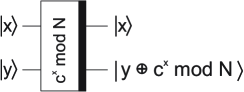
Figure 3: Operator for modular exponentiation

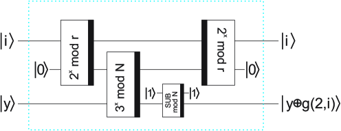
Figure 4: The circuit for $U$ using $x_{0}=2$.

Let us now describe the steps in the quantum period-finding algorithm, illustrated by Figure 5.

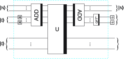
Figure 5: Perioding-finding using the $U$ operator of Figure 4 to factor $N$.

The initial state of the system is

$$|\Psi_{0}\rangle=|N\rangle_{n}|0\rangle_{\ell}|0\rangle_{n},$$

where $n=\lfloor\log_{2}N\rfloor+1$ is the number of bits needed to represent $N$ and $2^{\ell}$ is the number of elements evaluated by the operator QFT. In general, the size $\ell$ of the second register satisfies $N^{2}\leq 2^{\ell}<N^{2}+1$. See Shor [27] for more details. The ancilla bits are not shown in Figure 5.

After the Hadamard gates are applied, we get

$$|\Psi_{1}\rangle=|143\rangle_{n}H^{\otimes\ell}|0\rangle_{\ell}|0\rangle_{n}=\frac{1}{2^{\ell/2}}\sum_{i=0}^{2^{\ell}-1}|143\rangle_{n}|i\rangle_{\ell}|0\rangle_{n}.$$

Our strategy to restrict $g$ to the cycle, before $U$ is applied, is to give $g$ an initial value that is an element in the cycle, so we use the ADDER operator to shift the register $N$ units ahead, yielding

$$|\Psi_{2}\rangle=\frac{1}{2^{\ell/2}}\sum_{i=0}^{2^{\ell}-1}|143\rangle_{n}|143+i\rangle_{\ell}|0\rangle_{n}.$$

The ADDER operator is defined as $ADD\colon|A\rangle|B\rangle\rightarrow|A\rangle|A+B\rangle$. The size of the second register needs to be greater than or equal to the first register in this operator. See Vedral, Barenco and Eckert for more information about the implementation of the ADDER [29]. An extra q-bit $|0\rangle$ is needed to avoid a possible overflow. In our case, this extra q-bit is part of the second register of the ADDER, but the Hadamard gate is not applied to this q-bit. For simplicity, this bit is omitted in Figure 5 and in the description of the states of the system.

The next step is the application of $U$, after which the state of the system is

$$|\Psi_{3}\rangle=U|\Psi_{2}\rangle=\frac{1}{2^{\ell/2}}|143\rangle_{n}\sum_{i=0}^{2^{\ell}-1}|143+i\rangle_{\ell}|3^{2^{143+i}\bmod{15}}-1\bmod{143}\rangle_{n}.$$

For $N=143$, we have $2^{143}\equiv 2^{3}\bmod{15}$ and $n=8$. Taking $\ell=\lfloor\log_{2}(N^{2})\rfloor+1=15$, we get

$$|\Psi_{3}\rangle=\frac{1}{\sqrt{32768}}|143\rangle\sum_{i=0}^{32767}|143+i\rangle|3^{2^{3+i}\bmod{15}}-1\bmod{143}\rangle.$$

We can rewrite $|\Psi_{3}\rangle$ as

$$\begin{array}[]{rlll}|\Psi_{3}\rangle=\frac{1}{\sqrt{32768}}|143\rangle\bigl{(}&(|143\rangle+|147\rangle+|151\rangle+|155\rangle+\cdots+|32907\rangle)&|125\rangle&+\\ &(|144\rangle+|148\rangle+|152\rangle+|156\rangle+\cdots+|32908\rangle)&|2\rangle&+\\ &(|145\rangle+|149\rangle+|153\rangle+|157\rangle+\cdots+|32909\rangle)&|8\rangle&+\\ &(|146\rangle+|150\rangle+|154\rangle+|158\rangle+\cdots+|32910\rangle)&|80\rangle&\bigr{)}.\end{array}$$

The next step is the application of the reverse of the ADDER operator, after which we get

$$\begin{array}[]{rlll}|\Psi_{4}\rangle=\frac{1}{\sqrt{32768}}|143\rangle\bigl{(}&(|0\rangle+|4\rangle+|8\rangle+|12\rangle+\cdots+|32764\rangle)&|125\rangle&+\\ &(|1\rangle+|5\rangle+|9\rangle+|13\rangle+\cdots+|32765\rangle)&|2\rangle&+\\ &(|2\rangle+|6\rangle+|10\rangle+|14\rangle+\cdots+|32766\rangle)&|8\rangle&+\\ &(|3\rangle+|7\rangle+|11\rangle+|15\rangle+\cdots+|32767\rangle)&|80\rangle&\bigr{)}.\end{array}$$

The final state before measurement is $|\Psi_{5}\rangle=QFT^{\dagger}|\Psi_{4}\rangle$, that is,

$$|\Psi_{5}\rangle=\frac{1}{32768}|143\rangle\sum_{i=0}^{32767}\sum_{k=0}^{32767}e^{2\pi\iota ik/32768}|i\rangle|3^{2^{3+i}\bmod{15}}-1\bmod{143}\rangle,$$

where $\iota=\sqrt{-1}$.

We can use the principle of implicit measurement [23, box 5.4, page 235] to assume that the second register was measured, giving us a random result from {2, 8, 80, 125}. So, in this example, there are four possible outcomes of the measurement in the first register of the state $|\Psi_{5}\rangle$, all of which have the same probability of being measured. We might get either 0, 8192, 16384 or 24576, that is, $0/2^{\ell}$, $r_{\!g}/2^{\ell}$, $2r_{\!g}/2^{\ell}$ or $3r_{\!g}/2^{\ell}$, where $r_{\!g}=4$ is the period of the cycle produced by the function $g$. For more information on extracting $r_{\!g}$ from the measurement of $|\Psi_{5}\rangle$, please see Shor [27] and Nielsen, Chuang [23, section 5.3.1, page 226].

Finally, we compute $m=\gcd(g(N+r_{\!g}/2)-g(N),N)=\gcd(8-125,143)=13$, as desired.

11 Conclusions

John M. Pollard presented in 1975 an exponential algorithm for factoring integers that essentially searches the cycle of a sequence of natural numbers looking for a certain pair of numbers from which we can extract a nontrivial factor of the composite we wish to factor, assuming such pair exists. Until now there was no characterization of the pairs that yield a nontrivial factor. A characterization is now given by Theorem 4 in Section 5.

Peter W. Shor presented in 1994 a polynomial-time algorithm for factoring integers on a quantum computer that essentially computes the order $r$ of a number $x$ in the multiplicative group $\mathbb{Z}_{N}^{*}$ and uses $r$ to find a nontrivial divisor of the composite. No publication had so far reported that Shor’s strategy is essentially a particular case of Pollard’s strategy.

In the light of Theorem 4 in Section 5, we wrote a quantum version of Pollard’s Rho (Algorithm 2, Section 6) and Section 9 exposes the fact that by choosing a certain family of functions the steps of the algorithm are reduced to the exact steps of Shor’s algorithm.

References

- [1] Scott Aaronson “The limits of quantum” In Scientific American 298.3 JSTOR, 2008, pp. 62–69
- [2] Manindra Agrawal, Neeraj Kayal and Nitin Saxena “PRIMES is in P” In Annals of mathematics JSTOR, 2004, pp. 781–793
- [3] Stephane Beauregard “Circuit for Shor’s algorithm using 2n+3 qubits”, 2002 arXiv:quant-ph/0205095 [quant-ph]
- [4] David Beckman, Amalavoyal N. Chari, Srikrishna Devabhaktuni and John Preskill “Efficient networks for quantum factoring” In Phys. Rev. A 54 American Physical Society, 1996, pp. 1034–1063 DOI: 10.1103/PhysRevA.54.1034
- [5] Daniel J. Bernstein, Nadia Heninger, Paul Lou and Luke Valenta “Post-quantum RSA” In 8th International Workshop, PQCrypto2017, 2017, pp. 311–329 Springer
- [6] Richard P. Brent “An Improved Monte Carlo Factorization Algorithm” In BIT 20: 176–184, doi:10.1007/BF01933190, 1980
- [7] Zhengjun Cao “A Note on Shor’s Quantum Algorithm for Prime Factorization”, Cryptology ePrint Archive, Report 2005/051 URL: https://ia.cr/2005/051
- [8] Daniel Chicayban Bastos and Luis Antonio Kowada “How to detect whether Shor’s Algorithm succeeds against large integers without a quantum computer” In XI Latin and American Algorithms, Graphs and Optimization Symposium, 2021, pp. 132–138
- [9] Joachim Gathen and Jürgen Gerhard “Modern Computer Algebra” Cambridge University Press, 2013
- [10] Carl F. Gauss “Disquisitiones Arithmeticae” Springer-Verlag, 1986
- [11] Frédéric Grosshans, Thomas Lawson, François Morain and Benjamin Smith “Factoring Safe Semiprimes with a Single Quantum Query”, 2015 arXiv:1511.04385 [quant-ph]
- [12] Godfrey Harold Hardy and Edward Maitland Wright “An introduction to the theory of numbers” Oxford University Press, 1975
- [13] James L. Hein “Discrete Mathematics” JonesBartlett Publishers, 1996
- [14] Donald E. Knuth “The Art of Computer Programming, volume 2, seminumerical algorithms” Boston, MA, USA: Addison-Wesley Longman Publishing Co., Inc., 1997
- [15] Gary L. “Riemann’s Hypothesis and Tests for Primality” In Journal of computer and system sciences 13.3 Academic Press, 1976, pp. 300–317
- [16] Thomas Lawson “Odd orders in Shor’s factoring algorithm” In Quantum Information Processing 14.3 Springer, 2015, pp. 831–838
- [17] Gregor Leander “Improving the Success Probability for Shor’s Factoring Algorithm” In arXiv preprint quant-ph/0208183, 2002
- [18] Arjen K. Lenstra “Factoring” In International Workshop on Distributed Algorithms, 1994, pp. 28–38 Springer
- [19] Anna M. “Shor’s Algorithm and Factoring: Don’t Throw Away the Odd Orders”, Cryptology ePrint Archive, Report 2017/083, 2017 URL: https://ia.cr/2017/083
- [20] A.. Menezes, P.. Oorschot and S.. Vanstone “Handbook of Applied Cryptography”, Discrete Mathematics and Its Applications CRC Press, 1996
- [21] R.. Meter and K.. Itoh “Fast quantum modular exponentiation” In Physical Review A 71.5, 2005, pp. 052320
- [22] Michael A. Nielsen and Isaac L. Chuang “Quantum computation and quantum information”, Cambridge Series on Information and the Natural Sciences Cambridge University Press, 2004
- [23] Michael A. Nielsen and Isaac L. Chuang “Quantum computation and quantum information”, Cambridge Series on Information and the Natural Sciences Cambridge University Press, 2004
- [24] Carl Pomerance “Analysis and comparison of some integer factoring algorithms” In Computational methods in number theory Math. Centrum, 1982, pp. 89–139
- [25] Michael O. Rabin “Digitalized signatures and public-key functions as intractable as factorization”, 1979 URL: https://bit.ly/2WSjSXL
- [26] Ronald L. Rivest, Adi Shamir and Leonard Adleman “A Method for Obtaining Digital Signatures and Public-key Cryptosystems” In Commun. ACM 21.2 New York, NY, USA: ACM, 1978, pp. 120–126 DOI: 10.1145/359340.359342
- [27] Peter W. Shor “Polynomial-Time Algorithms for Prime Factorization and Discrete Logarithms on a Quantum Computer” In SIAM Journal on Computing 26.5 SIAM, 1997, pp. 1484–1509
- [28] Douglas Robert Stinson and Maura B. Paterson “Cryptography. Theory and Practice” CRC Press, 2018
- [29] V. Vedral, A. Barenco and A. Ekert “Quantum networks for elementary arithmetic operations” In Physical Review A 54.1, 1996, pp. 147–153
- [30] Peter W. “Algorithms for Quantum Computation: Discrete Logarithms and Factoring” In Proceedings of the 35th Annual Symposium on Foundations of Computer Science, SFCS ’94 Washington, DC, USA: IEEE Computer Society, 1994, pp. 124–134 DOI: 10.1109/SFCS.1994.365700
- [31] Peter W. “Polynomial-Time Algorithms for Prime Factorization and Discrete Logarithms on a Quantum Computer” In SIAM Journal on Computing 26.5 Society for Industrial & Applied Mathematics (SIAM), 1997, pp. 1484–1509 DOI: 10.1137/s0097539795293172
- [32] Peter W. “Polynomial-Time Algorithms for Prime Factorization and Discrete Logarithms on a Quantum Computer” In SIAM Review 41.2 SIAM, 1999, pp. 303–332
- [33] Samuel S. Wagstaff “The Joy of Factoring” American Mathematical Society, 2013
- [34] Guoliang Xu, Daowen Qiu, Xiangfu Zou and Jozef Gruska “Improving the Success Probability for Shor’s Factorization Algorithm” In Reversibility and Universality Springer, 2018, pp. 447–462