Contrastive Losses and Solution Caching for Predict-and-Optimize

Abstract

Many decision-making processes involve solving a combinatorial optimization problem with uncertain input that can be estimated from historic data. Recently, problems in this class have been successfully addressed via end-to-end learning approaches, which rely on solving one optimization problem for each training instance at every epoch. In this context, we provide two distinct contributions. First, we use a Noise Contrastive approach to motivate a family of surrogate loss functions, based on viewing non-optimal solutions as negative examples. Second, we address a major bottleneck of all predict-and-optimize approaches, i.e. the need to frequently recompute optimal solutions at training time. This is done via a solver-agnostic solution caching scheme, and by replacing optimization calls with a lookup in the solution cache. The method is formally based on an inner approximation of the feasible space and, combined with a cache lookup strategy, provides a controllable trade-off between training time and accuracy of the loss approximation. We empirically show that even a very slow growth rate is enough to match the quality of state-of-the-art methods, at a fraction of the computational cost.

1 Introduction

Many real-life decision-making problems can be formulated as combinatorial optimization problems. However, uncertainty in the input parameters is commonplace; an example being the day-ahead scheduling of tasks on machines, where future energy prices are uncertain. A predict-then-optimize Elmachtoub and Grigas (2021) approach is a widely-utilized industry practice, where first a machine learning (ML) model is trained to make a point estimate of the uncertain parameters and then the optimization problem is solved using the predictions.

The ML models are trained to minimize prediction errors without taking into consideration their impacts on the downstream optimization problem. This often results in sub-optimal decision performance. A more appropriate choice would be to integrate the prediction and the optimization task and train the ML model using a decision-focused loss Elmachtoub and Grigas (2021); Wilder et al. (2019); Demirović et al. (2019a). Such predict-and-optimize approach is proven to be effective in various tasks Mandi et al. (2020); Demirovic et al. (2019b); Ferber et al. (2020).

Unfortunately, computational complexity and scalability are two major roadblocks for the predict-and-optimize approach involving NP-hard combinatorial optimization problem. This is due to the fact that an NP-hard optimization problem must be solved and differentiated for each training instance on each training epoch to find a gradient of the optimization task and backpropgating it during model training.

A number of approaches Wilder et al. (2019); Ferber et al. (2020); Mandi and Guns (2020) consider problems formulated as Integer Linear program (ILP) and solve and differentiate the relaxed LP using interior point methods. On the other hand, the approaches from Mandi et al. (2020) and Pogančić et al. (2020) are solver-agnostic, because they compute a subgradient using solutions of any combinatorial solvers.

Here we propose an alternative approach, motivated by the literature of noise-contrastive estimation Gutmann and Hyvärinen (2010), which we use to develop a new family of surrogate loss functions based on viewing non-optimal solutions as negative examples. This necessitates building a cache of solutions, which we implement by storing previous solutions during training. We provide a formal interpretation of such a solution cache as an inner approximation of the convex-hull of feasible solutions. This is helpful whenever a linear cost vector is optimized over a discrete space. Our second contribution is to propose a family of loss functions specific to combinatorial optimization problems with linear objectives. As an additional contribution, we extend the concept of discrete inner approximation to solver-agnostic approaches. In this way, we are able to overcome the training time bottleneck. Finally, we empirically demonstrate that noise-contrastive estimation and solution caching produce predictions at the same quality or better than the state-of-the-art methods in the literature with a drastic decrease in computational times.

2 Related Work

Noise-contrastive estimation (NCE) performs tractable parameter optimization for many models requiring normalization of the probability distribution over a set of discrete assignments. This is a common element of many popular probabilistic logic frameworks like Markov Logic Networks Richardson and Domingos (2006) or Probabilistic Soft Logic Bach et al. (2017). More recently, NCE has been at the core of several neuro-symbolic reasoning approaches Garcez et al. (2012) like Deep Logic Models Marra et al. (2019) or Relational Neural Machines Marra et al. (2020). We use NCE to derive some tractable formulations of the combinatorial optimization problem.

Numerical instability is a major issue in end-to-end training as implicit differentiation at the optimal point leads to zero Jacobian when optimizing linear functions. Wilder et al. (2019) introduce end-to-end training of a combinatorial problem by constructing a simpler optimization problem in the continuous relaxation space adding a quadratic regularizer term to the objective. As the continuous relaxation is an outer approximation of the feasible region in mixed integer problems, Ferber et al. (2020) strengthen the formulation by adding cuts. Mandi and Guns (2020) propose to differentiate the homogeneous self-dual formulation, instead of the KKT condition and show its effectiveness.

The Smart Predict and Optimize (SPO) framework introduced by Elmachtoub and Grigas (2021) uses a convex surrogate loss based subgradient which could overcome the numerical instability issue for linear problems. Mandi et al. (2020) investigate scaling up the technique for large-scale combinatorial problems using continuous relaxations and warm-starting of the solvers. Recent work by Pogančić et al. (2020) is similar to the SPO framework but it uses a different subgradient considering “implicit interpolation” of the argmin operator. Both of these approaches are capable of computing the gradient for any blackbox implementation of a combinatorial optimization with linear objective. Elmachtoub et al. (2020) extends the SPO framework for decision trees.

In all the discussed approaches, scalability is a major challenge due to the need to repeatedly solve the (possibly relaxed) optimisation problems. In contrast, our contrastive losses, coupled with a solution caching mechanism, do away with repeatedly solving the optimization problem during training and can be applied to other solver agnostic predict-and-optimize methods, too.

3 Problem Setting

In our setting we consider a combinatorial optimization problem in the form

$$v^{*}(c)=\operatorname*{argmin}_{v\in V}f(v,c)$$ (1)

where $V$ is a set of feasible solutions and $f:V\times\mathcal{C}\rightarrow\mathbb{R}$ is a real valued function. The objective function $f$ is parametric in $c$, the values we will try to estimate. We denote by $v^{*}(c)$ an optimal solution of (1). Despite the fact that $V$ can be any set, for the rest of the article we will consider the particular case where $V$ is a discrete set, specified implicitly through a set of constraints. This type of sets arise naturally in combinatorial optimization problems, including Mixed Integer Programming (MIP) and Constraint Programming (CP) problems, many of which are known to be NP-complete.

The value of $c$ is unknown but we assume having access to correlated features $x$ and a historic dataset $D=\{(x_{i},c_{i})\}_{i=1}^{n}$. One straightforward method to learn $c$ is to find a model $m(\omega,x)$ with model parameters $\omega$ that predicts a value $\hat{c}$. This model can be learned by fitting the data $D$ to minimizing some loss function, as in classical supervised learning approaches.

In a predict-and-optimize setting, the challenge is to learn model parameters $\omega$, such that, when it is used to provide estimates $\hat{c}$, these predictions lead to an optimal solution of the combinatorial problem with respect to the real values of $c$. In order to measure how good a model is, we compute the regret of the combinatorial optimisation, that is, the difference between the true value of: 1) the optimal solution $v^{*}(c)$ for the true parameter values; and 2) the optimal solution for the estimated parameter values $v^{*}(\hat{c})$. Formally, $\mbox{Regret}(\hat{c},c)=f(v^{*}(\hat{c}),c)-f(v^{*}(c),c)$. In case of minimisation problems, regret is always positive and it is $0$ in case optimizing over the estimated values leads either to the true optimal solution or to an equivalent one.

The goal of prediction-and-optimisation is to learn the model parameters $\omega$ to minimize the regret of the resulting predictions, i.e. $\operatorname*{argmin}_{\omega}\mathbb{E}\left[\mbox{Regret}(m(\omega,x),c)\right]$. When using backpropagation as a learning mechanism, regret cannot be directly used as a loss function because it is non-continuous and involves differentiating over the argmin in $v^{*}(c)$. Hence, the general challenge of predict-and-optimize is to identify a differentiable and efficient-to-compute loss function $\mathcal{L}^{v^{*}}$ that takes into account the structure of $f$ and $v^{*}(\cdot)$ more generally.

Learning over a set of $N$ training instances can be formulated within the empirical risk minimisation framework as

$$\begin{split}\operatorname*{argmin}_{\omega}\mathbb{E}\left[\mathcal{L}^{v^{*}}(m(\omega,x),c)\right]\\ \approx\operatorname*{argmin}_{\omega}\frac{1}{N}\sum_{i=1}^{N}\mathcal{L}^{v^{*}}(m(\omega,x_{i}),c_{i})\end{split}$$ (2)

Algorithm 1 Gradient-descent over combinatorial problem

Input:$A$,$b$; training data D$\equiv\{(x_{i},c_{i})\}_{i=1}^{n}$
Hyperparams: $\alpha$- learning rate, epochs

1:  Initialize $\omega$.

2:  for each epochs do

3:     for each instances do

4:        $\tilde{c}\leftarrow t(\hat{c})$ with $\hat{c}=m(\omega,x)$

5:        Obtain $v$ by calling a solver for Eq. (1) with $\tilde{c}$

6:        $\omega\leftarrow\omega-\alpha\frac{\partial\mathcal{L}^{v}}{\partial\tilde{c}}\frac{\partial\tilde{c}}{\partial\omega}$ # backpropagate (sub)gradient

7:     end for

8:  end for

3.1 Gradient-Descent Decision-Focused Learning

Algorithm 1 depicts a standard gradient descent learning procedure for predict-and-optimize approaches. For each epoch and instance, it computes the predictions, optionally transforms them on Line 4, calls a solver to compute $v^{*}(\tilde{c})$, and updates the trainable weights $\omega$ via standard backpropagation for an appropriately defined gradient $\partial\mathcal{L}^{v}/\partial c$.

To overcome both the non-continuous nature of the optimisation problem $v^{*}(c)$ and the computation time required, a number of works replace the original task $v^{*}$ by a continuous relaxation $g^{*}$ and solve and implicitly differentiate over $\mathcal{L}^{g^{*}}$, considering a quadratic Wilder et al. (2019) or log-barrier Mandi and Guns (2020) task-loss. In these cases, $t(\hat{c})=\hat{c}$.

Other approaches are solver-agnostic and do the implicit differentiation by defining a subgradient for $\partial\mathcal{L}^{v}/\partial c$. In case of SPO+ loss Elmachtoub and Grigas (2021), the subgradient is $v^{*}(c)-v^{*}(2\hat{c}-c)$, involving $t(\hat{c})=(2\hat{c}-c)$. In case of Blackbox differentiation Pogančić et al. (2020), the solver is called twice on Line 5 of Alg 1 and the subgradient is an interpolation of $\mathcal{L}^{v}$ around $\hat{c}$, where the interpolation is between $v^{*}(\hat{c})$ and its perturbation $v^{*}(\hat{c}+\lambda c)$.

In all those cases, in order to find the (sub)gradient, the optimization problem $v^{*}(c)$ must be solved repeatedly for each instance. In the next section, we present an alternative class of contrastive loss functions that has, to the best of our knowledge, not been used before for predict-and-optimize problems. These loss functions can be differentiated in closed-form and do not require solving a combinatorial problem $v^{*}(c)$ for every instance.

4 A Contrastive Loss for Predict-and-Optimize

Probabilistic models define a parametric probability distributions over the feasible assignments, and Maximum Likelihood Estimation can be used to find the distribution parameters making the observed data most probable under the model Kindermann (1980). In particular, the family of exponential distributions emerges ubiquitously in machine learning, as it is the required form of the optimal solution of any maximum entropy problem Berger et al. (1996).

We now propose an exponential distribution that fits the optimisation problem of Eq. (1). Let $v\in V$ be the space of feasible output assignments $V$ for one example $x$. Then, we define the following exponential distribution over $V$:

$$p(v|m(\omega,x))=\frac{1}{Z}\exp\Big{(}-f(v,m(\omega,x))\Big{)}$$ (3)

the partition function Z normalizes the distribution over the assignment space $V$:

$$Z=\displaystyle\sum_{v^{\prime}\in V}\exp\Big{(}-f(v^{\prime},m(\omega,x))\Big{)}\ .$$

By construction, if $v^{*}(m(\omega,x))$ is the minimizer of Eq. 1 for an instance $x$, it will maximize Eq. (3) and vice versa. We can use this to fix the solution to $v=v^{*}(c)$ with $c$ being the true costs, and learn the network weights $\omega$ that maximize the likelihood $p(v^{*}(c)|m(\omega,x))$. This corresponds to learning an $\omega$ that makes the intended true solution $v^{*}(c)$ be the best scoring solution of Eq. 3 and hence of $v^{*}(m(\omega,x))$, which is the goal of prediction-and-optimisation. In the following, these definitions will be implicitly extended over all training instance ($x_{i},c_{i}$).

A main challenge of working with this distribution is that computing the partition function $Z$ requires iterating over all possible solutions $V$, which is intractable for most combinatorial optimization problems.

4.1 Noise-Contrastive Estimation

Learning over this distribution without a direct evaluation of $Z$ can be achieved by using Noise Contrastive Estimation (NCE) Mikolov et al. (2013). The key idea there is to work with a small set of negative samples. To apply NCE in this work, we will use as negative samples the solutions that are different from the target solution $v^{\star}$, that is any subset $S\subset(V\setminus v^{\star})$ of feasible solutions.

Such an NCE approach avoids a direct evaluation of $Z$ and instead maximizes the separation of the probability of the optimal solution ${v}^{\star}_{i}=v^{*}(c_{i})$ for $x_{i}$ from the probability of a sample of the non-optimal ones (the ‘noise’ part). It is expressed as a maximization of the product of ratios between the optimal solution $v^{\star}_{i}$ and the negative samples $S$:

$$\operatorname*{argmax}_{\omega}\log\prod_{i}\prod_{v^{s}\in S} \frac{p\Big{(}v^{\star}_{i}|m(\omega,x_{i})\Big{)}}{p\Big{(}v^{s}|m(\omega,x_{i})\Big{)}}=$$ (4)

$$=\operatorname*{argmax}_{\omega}\sum_{i}\sum_{v^{s}\in S} \Big{(}-f(v^{\star}_{i},m(\omega,x_{i}))-log(Z)$$

$$+f(v^{s},m(\omega,x_{i}))+log(Z)\Big{)}$$

$$=\operatorname*{argmax}_{\omega}\sum_{i}\sum_{v^{s}\in S} \Big{(}f(v^{s},m(\omega,x_{i}))-f(v^{\star}_{i},m(\omega,x_{i}))\Big{)}.$$

By changing the sign to perform loss minimization, this leads to the following NCE-based loss function:

$$\mathcal{L}_{\operatorname*{NCE}}=\sum_{i}\sum_{v^{s}\in S}\Big{(}f\big{(}v^{\star}_{i},m(\omega,x_{i})\big{)}-f\big{(}v^{s},m(\omega,x_{i}\big{)}\Big{)}$$ (5)

which can be plugged directly into Algorithm 1. During differentiation, both $v^{\star}_{i}$ and $v^{s}$ will be treated as constants- the first since it effectively never changes, the second since it will be computed in the forward pass on line 5 in Alg. 1. As a side effect, automatic differentiation of Eq. 5 will yield a subgradient rather than a true gradient, as is common in integrated predict-and-optimize settings. In section 5, we will discuss how to create the sample $S$.

4.2 MAP Estimation

Self-contrastive estimation Goodfellow (2015) is a special case of NCE where the samples are drawn from the model. A simple but very efficient self-contrastive algorithm takes a single sample, which is the Maximum A Posteriori (MAP) assignment, i.e. the most probable solution for each example according to the current model $m(\omega,\cdot)$. Therefore , the MAP assignment approximation trains the weights $\omega$ as:

$$\operatorname*{argmax}_{\omega}\displaystyle\sum_{i}\left[-f(v^{\star}_{i},m(\omega,x_{i}))+f(\hat{v}^{\star}_{i},m(\omega,x_{i}))\big{]}\right]$$

with $\hat{v}^{\star}_{i}=\operatorname*{argmin}_{v^{\prime}\in S}[f(v^{\prime},m(\omega,x_{i}))]$ being the MAP solution for the current model. With a sign change to switch optimization direction, this translates into the following loss variant:

$$\mathcal{L}_{\operatorname*{MAP}}=\displaystyle\sum_{i}\big{[}f(v^{\star}_{i},m(\omega,x_{i}))-f(\hat{v}^{\star}_{i},m(\omega,x_{i}))\big{]}$$ (6)

4.3 Better Handling of Linear Cost Functions

The losses can be minimized by either matching the true optimal solution (the intended behavior), or by making $f\left(v^{\star}_{i},m(\omega,x_{i})\right)$ and $f\left(\hat{v}^{\star}_{i},m(\omega,x_{i})\right)$ identical by other means. For example, with a linear cost function $f(v,c)=c^{T}v$, Eq. 5 translates to:

$$\mathcal{L}_{\operatorname*{NCE}}=\sum_{i}\sum_{v^{s}\in S}m(\omega,x_{i})^{T}(v^{\star}_{i}-v^{s})$$ (7)

which can be minimized by predicting null costs, i.e. $m(\omega,x_{i})=0$. To address this issue, we introduce a variant of Eq. 5, where we replace the $\hat{c_{i}}$ term in the loss with $\big{(}\hat{c_{i}}-c_{i}\big{)}$. The modification amounts to adding a constant (so that all optimal solutions are preserved), and can be viewed as a regularization term that keeps $\hat{c}$ close to $c$. Thus we get:

$$\mathcal{L}_{\operatorname*{NCE}}^{(\hat{c}-c)} =\sum_{i}\sum_{v^{s}\in S}\Big{(}(m(\omega,x_{i})-c_{i})^{T}(v^{\star}_{i}-v^{s})\Big{)}$$ (8)

where $\hat{c}$ (in the loss name) is a shorthand for $m(\omega,x_{i})$. Note that we do not perturb the predictions prior to computing $\hat{v}^{\star}_{i}$, but only in the loss function.

The loss is still guaranteed non-negative, since $v^{\star}_{i}$ is by definition the best possible solution with the cost vector $c_{i}$. Eq. 7 can no longer be minimized with a null cost vector; instead, the loss can only be minimized by having the predicted costs $\hat{c}_{i}$ match the true costs $c_{i}$ or, and implied by that, having the solution with the estimated parameters $\hat{v}^{\star}_{i}$ match the true optimal solution $v^{\star}_{i}$. The same approach applied to the MAP version leads to:

$$\mathcal{L}_{\operatorname*{MAP}}^{(\hat{c}-c)}=\sum_{i}(m(\omega,x_{i})-c_{i})^{T}(v^{\star}_{i}-\hat{v}^{\star}_{i})$$ (9)

5 Negative Samples and Inner-approximations

5.1 Negative Sample Selection

The main question now is how to select the ‘noise’, i.e. the negative samples $S$. The only requirement is that any example in $S$ is a feasible solution, i.e. $S\subseteq V$. Instead of computing multiple feasible solutions in each iteration, which would be more costly, we instead propose the pragmatic approach of storing each solution found when calling the solver on Line 5 of Alg. 1 in a solution cache. As training proceeds, the solution cache will grow each time a new solution is found, and we can use this solution cache as negative samples $S$.

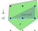
Figure 1: Representation of a solution cache (blue) and the continuous relaxation (green) of $V$.

While pragmatic, we can also interpret this solution cache $S$ from a combinatorial optimisation perspective: if $S$ would contain all possibly optimal solutions (for linear cost functions), it would represent the convex hull of the entire feasible space $V$. When containing only a subset of points, that is, a subset of the convex hull, it can be seen as an inner approximation of $V$. This in contrast to continuous relaxation that relax the integrality constraints, which are commonly used in prediction-and-optimisation today, that lead to an outer approximation. The inner approximation has the advantage of having more information about the structure of $V$. This is depicted in Figure 1 where a solution cache $S$ is represented by blue points, and the set $V$ of feasible points is the union of black and blue points. The continuous relaxation of this set depends on the formulation, that is, the precise set of inequalities used to represent $V$, for example, the green part, which clearly is an outer approximation of the convex-hull of $V$. The convex-hull of the solution cache is represented as $conv(S)$ and it is completely included in $conv(V)$ in contrast to the outer approximation.

5.2 Gradient-descent with Inner Approximation

The idea that caching the computed solutions results in an inner approximation, is not limited to noise-contrastive estimation. As $S$ becomes larger we can expect the inner approximation to become tighter, and hence we can solve the inner approximation instead of the computationally expensive full problem. Because the inner approximation is a reasonably sized list of solutions, solving it simply corresponds to a linear-time argmin over this list!

Algorithm 2 Gradient-descent with inner approximation

Input:$A$,$b$; training data D$\equiv\{(x_{i},c_{i})\}_{i=1}^{n}$
Hyperparams: $\alpha$ learning rate, epochs, $p_{solve}$

1:  Initialize $\omega$

2:  Initialize $S=\{v^{*}(c_{i})|(x_{i},c_{i})\in D\}$

3:  for each epochs do

4:     for each instances do

5:        $\tilde{c}\leftarrow t(\hat{c})$ with $\hat{c}=m(\omega,x)$

6:        if random$()<p_{solve}$ then

7:           Obtain $v$ by calling a solver for Eq. (1) with $\tilde{c}$

8:           $S\leftarrow S\cup\{v\}$

9:        else

10:           $v=\operatorname*{argmin}_{v^{\prime}\in S}(f(v^{\prime},\tilde{c}))$ // simple argmin

11:        end if

12:        $\omega\leftarrow\omega-\alpha\frac{\partial\mathcal{L}^{v}}{\partial\tilde{c}}\frac{\partial\tilde{c}}{\partial\omega}$ # backpropagate (sub)gradient

13:     end for

14:  end for

Alg. 2 shows the generic algorithm. In comparison to Alg. 1 the main difference is that on Line 2 we initialise the solution pool, for example with all true optimal solutions; these must be computed for most loss functions anyway. On Line 6 we now first sample a random number between 0 and 1, and if it is below $p_{solve}$, which represents the probability of calling the solver, then the expensive solver is called and the solution is added to the cache if not yet present, otherwise an argmin of the cache is done.

	Knapsack 60	Knapsack 120	Knapsack 180
$\mathcal{L}_{\operatorname*{NCE}}$ $\hat{c}$	912(21)	760(12)	2475(45)
$\mathcal{L}_{\operatorname*{NCE}}$ $(\hat{c}-c)$	1024(66)	770(15)	2474 (40)
$\mathcal{L}_{\operatorname*{MAP}}$ $\hat{c}$	1277(555)	912(9)	491(8)
$\mathcal{L}_{\operatorname*{MAP}}$ $(\hat{c}-c)$	764 (2)	562(1)	327(1)
Two-stage	989 (14)	1090 (27)	433 (12)

Table 1: Comparison among Contrastive loss variants on Knapsacks (Average and standard deviation of regret on test data)

	Energy 1	Energy 2	Energy 3
$\mathcal{L}_{\operatorname*{NCE}}$ $\hat{c}$	45847 (780)	27633 (214)	18789 (194)
$\mathcal{L}_{\operatorname*{NCE}}$ $(\hat{c}-c)$	45834 (1657)	28994 (659)	18768 (406)
$\mathcal{L}_{\operatorname*{MAP}}$ $\hat{c}$	104496 (18109)	50897 (20958)	32180 (8382)
$\mathcal{L}_{\operatorname*{MAP}}$ $(\hat{c}-c)$	41236 (66)	27734 (267)	17507 (42)
Two-stage	43384 (376)	31798 (781)	23423 (893)

Table 2: Comparison among Contrastive loss variants on Energy scheduling (Average and standard deviation of regret on test data)

	Matching 10	Matching 25	Matching 50
$\mathcal{L}_{\operatorname*{NCE}}$ $\hat{c}$	3702 (64)	3696 (76)	3382 (49)
$\mathcal{L}_{\operatorname*{NCE}}$ $(\hat{c}-c)$	3618 (81)	3674 (48)	3376 (73)
$\mathcal{L}_{\operatorname*{MAP}}$ $\hat{c}$	3708 (88)	3700 (23)	3444 (74)
$\mathcal{L}_{\operatorname*{MAP}}$ $(\hat{c}-c)$	3732 (85)	3712 (86)	3402 (66)
Two-stage	3700 (42)	3712 (59)	3440 (36)

Table 3: Comparison among Contrastive loss variants on Diverse Bipartite Matching (Average and standard deviation of regret on test data)

Note how the probability of solving $p_{solve}$ has an efficiency-accuracy trade-off: more solving is computationally more expensive but leads to better approximations of V. The approach of Alg. 1 corresponds to $p_{solve}=1$.

This inner-approximation caching approach can be used for any decision-focused learning method that calls an external solver, such as SPO+ method in Mandi et al. (2020) and its variants Elmachtoub et al. (2020), Blackbox solver differentiation of  Pogančić et al. (2020) and our two contrastive losses $\mathcal{L}_{\operatorname*{MAP}}$ and $\mathcal{L}_{\operatorname*{NCE}}$.

6 Empirical Evaluation

In this section we answer the following research questions:

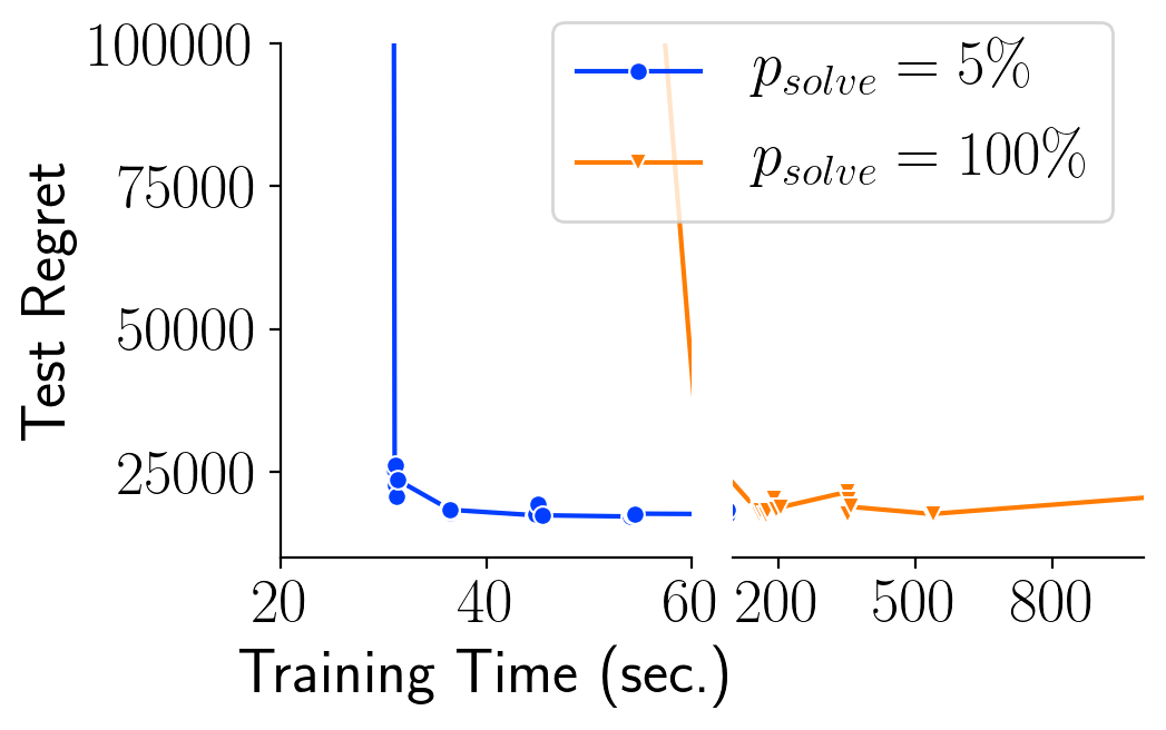
(a) NCE

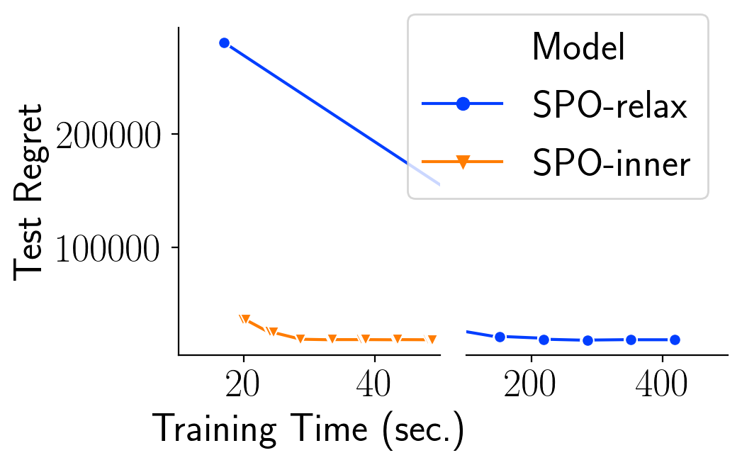
(b) SPO+

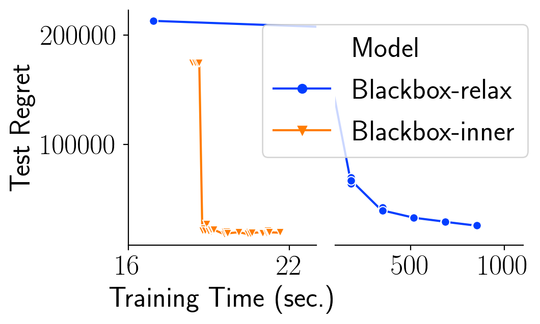
(c) Blackbox

Figure 2: Comparison of learning curves with/without the inner approximation with $p_{solve}=5\%$ for Energy-3.

• What is the performance of each task loss function in terms of expected regret?

• How does the growth of the solution caching impact on the solution quality and efficiency of the learning task?

• How do other solver-agnostic methods benefit from the solution caching scheme?

• How does the methodology outlined above perform in comparison with the state-of-the-art algorithms for decision-focused learning?

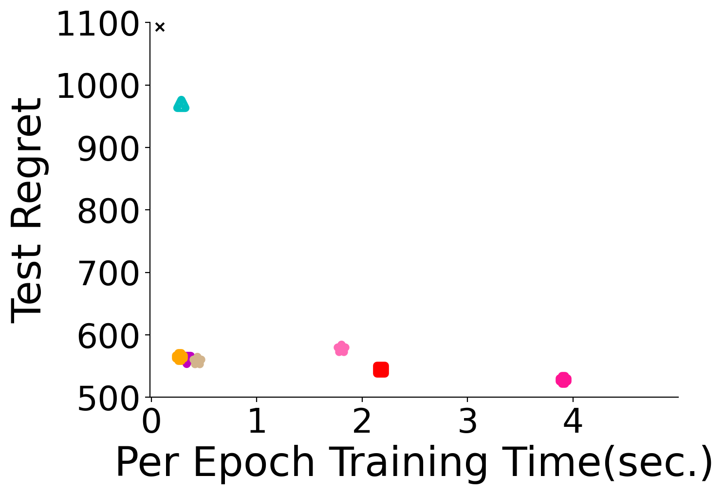
(a) Knapsack-120

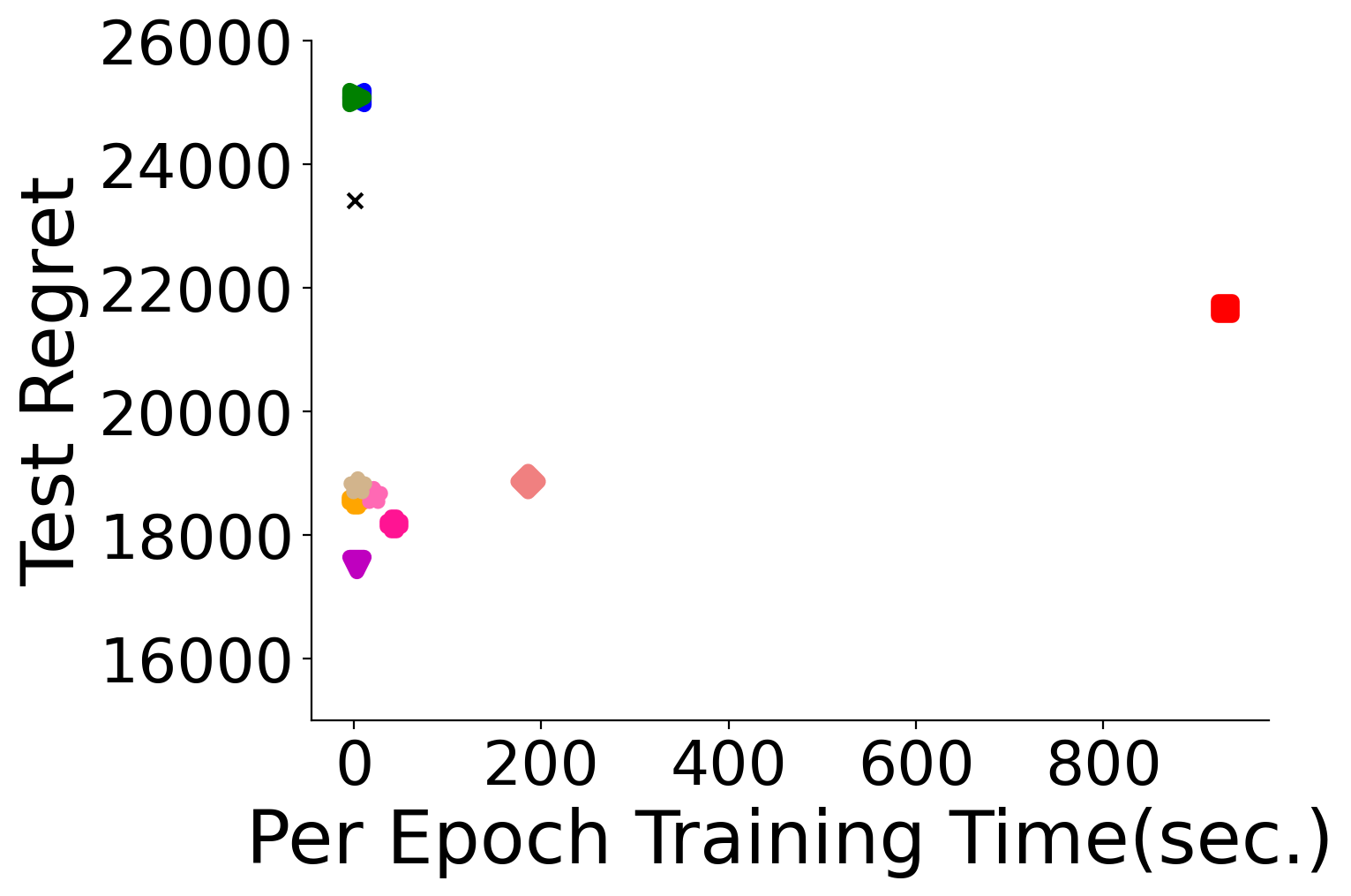
(b) Energy-3

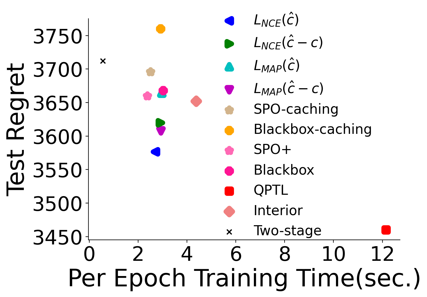
(c) Matching-25

Figure 3: Regret versus total training time for the different methods

To do so, we evaluate our methodology on three NP hard problems, the knapsack problem, a job scheduling problem and a maximum diverse bipartite matching problem.

6.1 Experimental Settings

Knapsack Problem.

The objective of this problem is to select a maximal value subset from a set of items subject to a capacity constraint. We generate our dataset from Ifrim et al. (2012), which contains historical energy price data at 30-minute intervals from 2011-2013. Each half-hour slot has features such as calendar attributes; day-ahead estimates of weather characteristics; SEMO day-ahead forecasted energy-load, wind-energy production and prices. Each knapsack instance consists of $48$ half-our slots, which basically translates to one calendar day. The knapsack weights are synthetically generated where a weight $\in\{3,5,7\}$ is randomly assigned to each of the 48 slots and the price is multiplied accordingly before adding Gaussian noise $\xi\sim\mathbb{N}(0,25)$ to maintain high correlation between the prices and the weights as strongly correlated instances are difficult to solve Pisinger (2005). We study three instances of this knapsack problem with capacities of 60, 120 and 180.

Energy-cost Aware Scheduling.

In our next experiment, we consider a more complex combinatorial optimization problem. This combinatorial problem is taken from CSPLib Gent and Walsh (1999), a library of constraint optimization problems. In energy-cost aware scheduling Simonis et al. (1999), a given number of tasks, each having its own duration, power usage, resource requirement, earliest possible start and latest-possible end, must be scheduled on a certain number of machines respecting the resource capacities of the machines. A task cannot be stopped or migrated once started on a machine. The cost of energy price varies throughout the day and the goal is to find a scheduling which would minimize the total energy consumption cost. We use the same energy price data for this experiment. We study three instances named Energy-1, Energy-2 and Energy-3.

Diverse Bipartite Matching.

We adopt this experiment from Ferber et al. (2020). The matching instances are constructed from the CORA citation network Sen et al. (2008). The graph is partitioned into 27 sets of disjoint nodes. Diversity constraints are added to ensure there are some edges between papers of the same field as well as edges between papers of different fields. The prediction task is to predict which edges are present using the node features. The optimization task is to find a maximum matching in the predicted graph. Contrary to the previous ones, here the learning task is the challenging one whereas the optimisation task is relatively simpler. We study three instances with varying degree of diversity constraints, Matching-10, Matching-25 and -50.

6.2 Results

For all the experiments, the dataset is split on training ($70\%$), validation ($10\%$) and test ($20\%$) data. The validation sets are used for selecting the best hyperparameters. The final model is run on the test data 10 times and we report the average and standard deviation (in bracket) of the 10 runs. All methods are implemented with Pytorch 1.3.1 Paszke et al. (2019) and Gurobi 9.0.1 Gurobi Optimization (2021).

6.2.1 Q1

In section 4, we introduced $\mathcal{L}_{\operatorname*{NCE}}$, $\mathcal{L}_{\operatorname*{MAP}}$, $\mathcal{L}_{\operatorname*{NCE}}^{(\hat{c}-c)}$ and $\mathcal{L}_{\operatorname*{MAP}}^{(\hat{c}-c)}$. In Table 1, 2 and 3, we compare the test regret of these 4 contrastive losses. The test regret of a two-stage approach, where model training is done with no regards to the optimization task, is provided as baseline.

We can see in Table 1 and Table2 for the knapsack and the scheduling problem, $\mathcal{L}_{\operatorname*{MAP}}\ (\hat{c}-c)$ performs the best among all the loss variants. Interestingly, with $\mathcal{L}_{\operatorname*{NCE}}$, there is no significant advantage of the linear objective loss function ($\hat{c}-c)$); whereas in case of $\mathcal{L}_{\operatorname*{MAP}}$, we observe significant gain by using the linear objective loss function. On the other hand, in Table 3, for the matching problem $\mathcal{L}_{\operatorname*{NCE}}$ performs slightly better than $\mathcal{L}_{\operatorname*{MAP}}$.

6.2.2 Q2

In the previous experiment, the initial discrete solutions on the training data as well as all solutions obtained during training are cached to form the inner approximation of the feasible region. But, as explained in section 5, finding the optimal $v^{*}(\hat{c})$ and adding it to the solution cache for all $\hat{c}$ during training is computationally expensive. Instead, now we empirically experiment with $p_{solve}=5\%$, i.e. where new solutions are computed only $5\%$ of the time.

In Figure 2(a), we plot regret against training time for Energy-3 (we observe similar results as shown in the appendix). There is a significant reduction in computational times as we switch to $5\%$ sampling strategy. Moreover, this does have not deleterious impact on the test regret. We conclude that adding new solutions to the solution cache by sampling seem to be an effective strategy to have good quality solutions without a high computational burden.  

6.2.3 Q3

To investigate the validity of inner-approximation caching approach, we implement SPO-caching and Blackbox-caching, where we perform differentiation of SPO+ loss and Blackbox solver differentiation respectively, with $p_{solve}$ being $5\%$. We again plot regret against training time in Figure 2(b) and Figure 2(c) for SPO+ and Blackbox respectively. These figures show caching drastically reduces training times without any significant impact on regret both for SPO+ and Blackbox differentiation.

6.2.4 Q4

Finally we investigate what we gain by implementing $\mathcal{L}_{\operatorname*{NCE}}$, $\mathcal{L}_{\operatorname*{NCE}}^{(\hat{c}-c)}$, $\mathcal{L}_{\operatorname*{MAP}}^{(\hat{c}-c)}$ and SPO-caching and blackbox-caching with $p_{solve}$ being $5\%$. We compare them against some of the state-of-the-art approaches- SPO+ Elmachtoub and Grigas (2021); Mandi et al. (2020), Blackbox Pogančić et al. (2020), QPTL Wilder et al. (2019) and Interior Mandi and Guns (2020). Our goal is not to beat them in terms of regret; rather our motivation is to reach similar regret in a time-efficient manner.

In Figure 3(a), Figure 3(b) and 3(c), we plot Test regret against per epoch training time for Knapsack-120, Energy-3 and Matching-25. In Knapsack-120, Blackbox and Interior performs best in terms of regret. $\mathcal{L}_{\operatorname*{MAP}}^{(\hat{c}-c)}$, SPO-caching and Blackbox-caching attain low regret comparable to these with a significant gain in training time. For Energy-3 the regret of SPO-caching and Blackbox-caching are comparable to the state of the art, whereas $\mathcal{L}_{\operatorname*{MAP}}^{(\hat{c}-c)}$, in this specific case, results in lowest regret at very low training time. In Matching-25, QPTL is the best albeit the slowest and SPO+ and Blackbox perform marginally better than a two-stage approach. In this instance, caching methods are not good enough; but the four contrastive methods performs better than SPO+ and Blackbox. These methods can be viewed as trade-off between lower regret of QPTL and faster runtime of two-stage.

7 Concluding Remarks

We presented a methodology for decision-focused learning based on two main contributions: i. A new family of loss functions inspired by noise contrastive estimation; and ii. A solution cache representing an inner approximation of the feasible region. We adapted the solution caching concept to other state-of-the-art methods, namely Blackbox Pogančić et al. (2020) and SPO+ Elmachtoub and Grigas (2021), for decision-focused learning improving their efficiency. These two concepts allow to reduce solution times drastically while reaching similar quality solutions.

Appendix A Predictive models

For knapsack and scheduling experiments, we train a simple linear regressor implemented as a single layer network in PyTorch, trained to minimize Mean Square Error. For matching experiments, we consider a 2-layers perceptron with an hidden layer of 200 units and ReLU activation function. As it is used in a binary classification problem, we apply a sigmoid function on its output. The neural network is trained to minimize Cross Entropy.

All predictive model are trained with ADAM Kingma and Ba [2015].

Appendix B Detailed Result

		Two-stage	SPO	Blackbox	QPTL	Interior	SPO-caching (5$\%$)	Blackbox-caching (5$\%$)
Knapsack-60	Regret	989 (14)	734 (10)	659 (15)	668 (4)	700 (54)	730 (42)	682 (37)
	MSE	34101(115)	$10^{6}$ (105)	$1.5\times 10^{6}$ (18)	$10^{6}$ (533)	$1.5\times 10^{6}$ (232)	$10^{6}$ (8$\times 10^{3}$)	$1.5\times 10^{6}$ (44)
Knapsack-120	Regret	1090 (27)	578 (1)	528 (10)	545 (1)	565 (40)	558 (7)	565 (40)
	MSE	34107(79)	$10^{6}$ (50)	$1.5\times 10^{6}$ (40)	$1.5\times 10^{6}$ (37)	$1.5\times 10^{6}$ (280)	$10^{6}$ ($10^{3}$)	$1.5\times 10^{6}$ (36)
Knapsack-180	Regret	433 (12)	316 (1)	314 (13)	1461 (13)	370 (22)	354 (14)	316 (22)
	MSE	34145(80)	$0.5\times 10^{6}$ (33)	$1.5\times 10^{6}$ (16)	$1.5\times 10^{6}$ (44)	$1.5\times 10^{6}$ (260)	$10^{6}$ ($10^{3}$)	$1.5\times 10^{6}$ (64)

Table 4: Test Regret of the state of the art for the Knapsack Problem

	SPO	SPO-caching (5$\%$)	Blackbox	Blackbox-caching (5$\%$)
Knapsack-60	2	0.5	4.5	0.5
Knapsack-120	2	0.5	4	0.5
Knapsack-180	2	0.5	4	0.5

Table 5: Per Epoch Runtime (sec.) of the caching implementation for the Knapsack Problem

$\mathcal{L}_{\operatorname*{NCE}}$

$\mathcal{L}_{MAP}$

$\hat{c}$

$(\hat{c}-c)$

$(2\hat{c}-c)$

$\hat{c}$

$(\hat{c}-c)$

$(2\hat{c}-c)$

Knapsack-60

Regret

912 (21)

1024 (66)

908 (15)

1277 (555)

764 (2)

809 (2)

MSE

$10^{6}$ (2$\times 10^{3}$)

$1.5\times 10^{6}$ (425)

$10^{6}$ ($10^{3}$)

$1.5\times 10^{6}$ (2)

$10^{6}$ (395)

$10^{6}$ (287)

Knapsack-120

Regret

760 (12)

770 (15)

763 (10)

912 (9)

562 (1)

591 (2)

MSE

$1.5\times 10^{6}$ (3)

$1.5\times 10^{6}$ (3)

$1.5\times 10^{6}$ (2)

$1.5\times 10^{6}$ (1)

$10^{6}$ (292)

$10^{6}$ (264)

Knapsack-180

Regret

2475 (45)

2474 (40)

2478 (630)

491 (8)

327 (1)

331 (5)

MSE

$10^{6}$ (47)

$10^{6}$ (62)

$10^{6}$ (24)

$1.5\times 10^{6}$ (1)

40500 (200)

52000 (158)

Table 6: Test Regret of the Variants of the Knapsack Problem

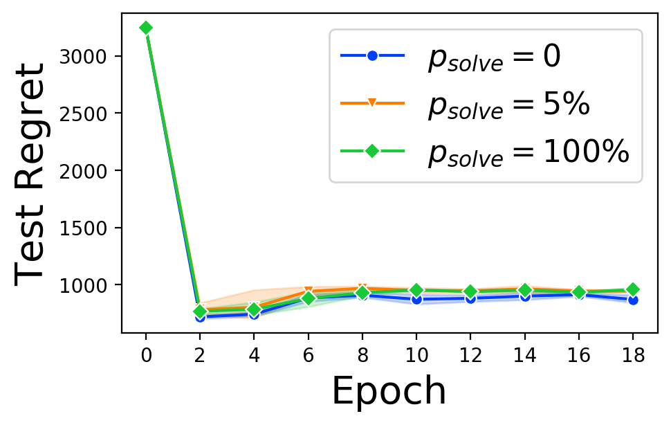
(a) Knapsack-60

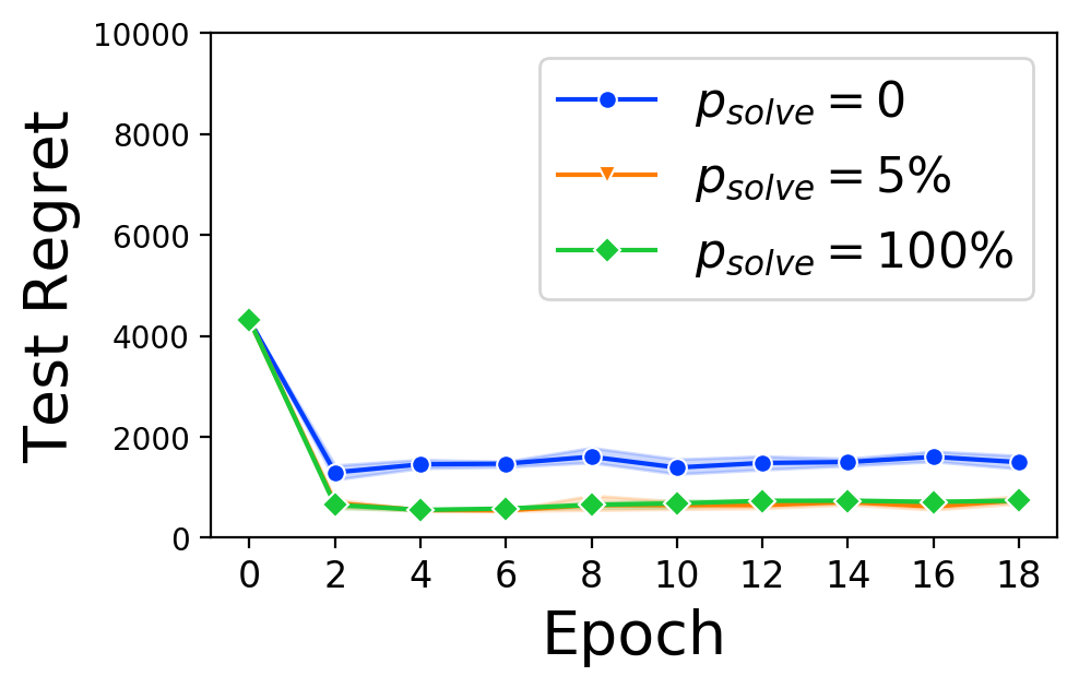
(b) Knapsack-120

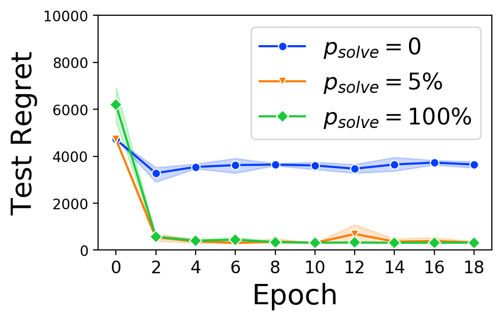
(c) Knapsack-180

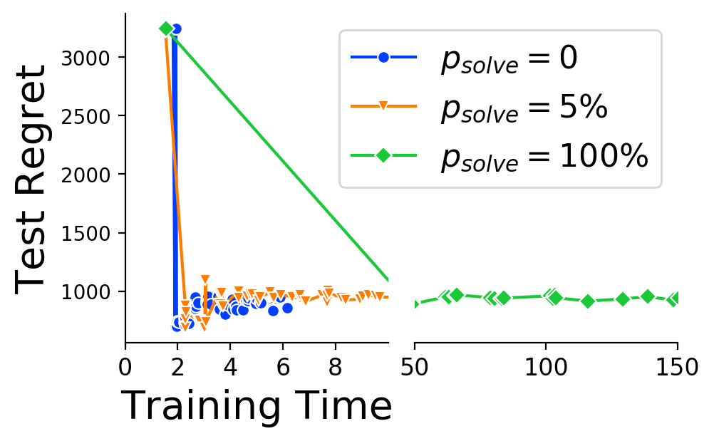
(d) Knapsack-60

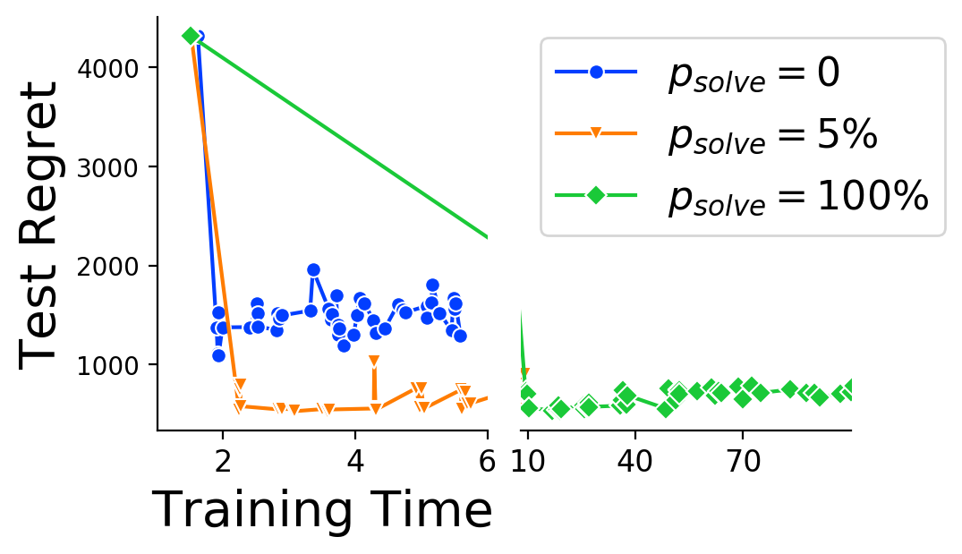
(e) Knapsack-120

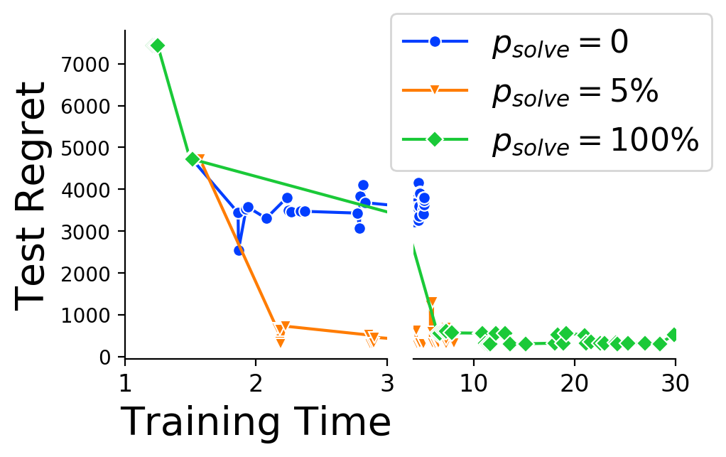
(f) Knapsack-180

Figure 4: Learning Curve for Knapsack Problem
$\mathcal{L}_{MAP}$ $(\hat{c}-c)$

		Two-stage	SPO-relax	Blackbox	QPTL	Interior	SPO-caching (5$\%$)	Blackbox-caching (5$\%$)
Energy-1	Regret	43384 (376)	40935 (115)	38800 (79)	40615 (799)	40200 (225)	40820 (76)	41635 (781)
	MSE	769 (3)	9648 (148)	5432 (2)	5161 (1)	2334 (66)	14464 (434)	5612 (42))
Energy-2	Regret	31978 (781)	27470 (42)	27405 (144)	37639 (194)	29407 (1855)	27591 (77)	27776 (856)
	MSE	768 (3)	5582 (248)	5525 (2)	5436 (1)	3651 (47)	10654 (664)	5571 (31)
Energy-3	Regret	23423 (893)	18647 (234)	18187 (587)	21677 (857)	18509 (1121)	18803 (39)	18881 (1481)
	MSE	770 (3)	3237 (37)	5485 (5)	5208 (4)	3742 (67)	5008 (229)	5455 (32)

Table 7: Test Regret of the state of the art of the Energy Scheduling Problem

	SPO	SPO-caching (5$\%$)	Blackbox	Blackbox-caching (5$\%$)
Energy-1	6.5	2	14	1
Energy-2	12	2	26.5	0.5
Energy-3	21	3.5	42.5	1.5

Table 8: Per Epoch Runtime (sec.) of the caching implementation for the Energy Scheduling Problem

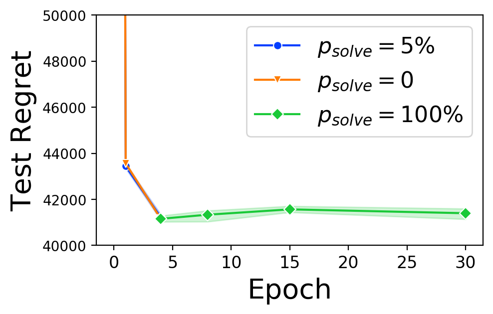
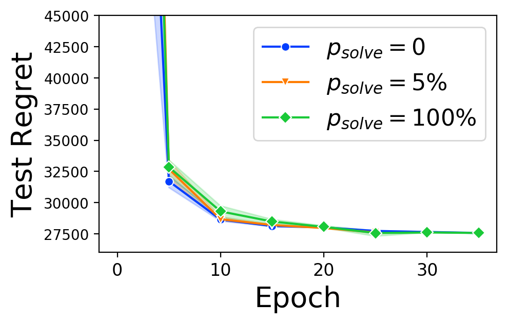
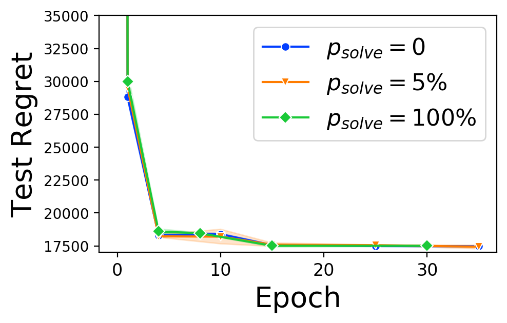
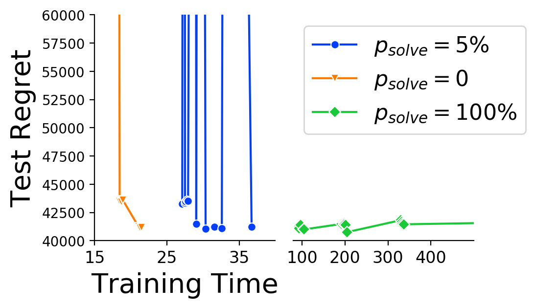
(a) Energy-1

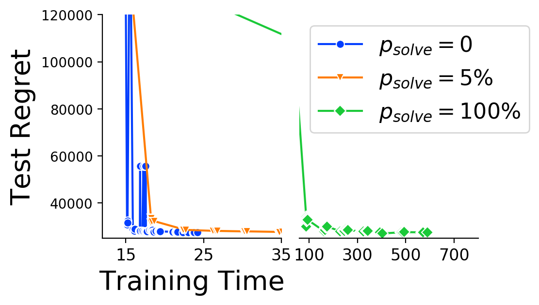
(b) Energy-2

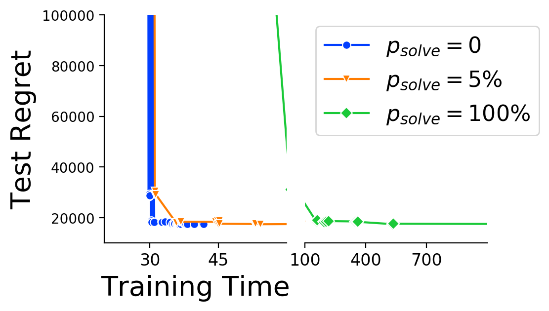
(c) Energy-3

Figure 5: Learning Curve for Energy Scheduling Problem
$\mathcal{L}_{MAP}$ $(\hat{c}-c)$

		$\mathcal{L}_{\operatorname*{NCE}}$			$\mathcal{L}_{MAP}$
		$\hat{c}$	$(\hat{c}-c)$	$(2\hat{c}-c)$	$\hat{c}$	$(\hat{c}-c)$	$(2\hat{c}-c)$
Energy-1	Regret	45847(780)	45834(1657)	51504(339)	104496 (18109)	41236 (66)	40762 (85)
	MSE	5477(5)	5475(4)	5352(268)	19070(291)	12958(1753)	15133(1164)
Energy-2	Regret	27633(214)	28994(659)	29339(681)	50897(20958)	27734 (267)	27728(346)
	MSE	5578(55)	17146(2620)	17864(3613)	6190(14)	10528(945)	11580(858)
Energy-3	Regret	18789(194)	18768(406)	18665(630)	32180(8382)	17507(42)	17504(156)
	MSE	14528(578)	14814(742)	13691(1572)	5876(36)	33593(4992)	49130(13108)

Table 9: Test Regret of the Variants of the Energy Scheduling Problem

		Two-stage	SPO	Blackbox	QPTL	Interior	SPO-caching (5$\%$)	Blackbox-caching (5$\%$)
Matching-10	Regret	3700 (42)	3746 (54)	3642 (73)	3422 (80)	3788 (58)	3664 (140)	3704 (74)
	AUC	0.497 (0.001)	0.492 (0.010)	0.483 (0.003)	0.586 (0.019)	0.495 (0.015)	0.480 (0.001)	0.495 (0.005)
Matching-25	Regret	3712 (59)	3786 (85)	3710 (65)	3482 (71)	3652 (87)	3696 (85)	3760 (57)
	AUC	0.495 (0.001)	0.494 (0.014)	0.503 (0.006)	0.569 (0.016)	0.501 (0.003)	0.498 (0.004)	0.498 (0.013)
Matching-50	Regret	3440 (36)	3458 (61)	3314 (76)	3242 (75)	3524 (117)	3416 (70)	3440 (28)
	AUC	0.494 (0.003)	0.510 (0.012)	0.525 (0.004)	0.564 (0.011)	0.485 (0.002)	0.507 (0.003)	0.490 (0.008)

Table 10: Test Regret of the state of the art for the Diverse Bipartite Matching Problem

		$\mathcal{L}_{\operatorname*{NCE}}$				$\mathcal{L}_{MAP}$
		$\hat{c}$	$(\hat{c}-c)$	$(2\hat{c}-c)$		$\hat{c}$	$(\hat{c}-c)$	$(2\hat{c}-c)$
Matching-10	Regret	3702 (64)	3618 (81)	3710 (45)		3708 (88)	3732 (85)	3692 (63)
	AUC	0.486 (0.003)	0.487 (0.004)	0.488 (0.007)		0.495 (0.002)	0.493 (0.004)	0.492 (0.002)
Matching-25	Regret	3696 (76)	3674 (48)	3736 (74)		3700 (23)	3712 (86)	3760 (60)
	MSE	0.496 (0.004)	0.495 (0.002)	0.496 (0.006)		0.494 (0.002)	0.490 (0.005)	0.494 (0.004)
Matching-50	Regret	3382 (49)	3376 (73)	3396 (57)		3444 (74)	3402 (66)	3380 (86)
	AUC	0.513 (0.004)	0.517 (0.005)	0.512 (0.003)		0.499 (0.002)	0.509 (0.01)	0.506 (0.007)

Table 11: Test Regret of the Variants of the Diverse Bipartite Matching Problem

Appendix C Problem Specification

C.1 Knapsack problem

In this problem we have to predict electricity-price $c_{t}$ of $T$(= 48) half-hour slots of the next day. Each slot $t$, is associated with a known weight $w_{t}$, which can be interpreted as the agency fee of that slot. The problem of maximizing the total revenue is stated as the following MILP:

$$\max_{x} \sum_{t\in T}c_{t}x_{t}$$

subject to $$\sum_{t\in T}w_{t}x_{t}\leq B$$

$$x_{t}\in\{0,1\} t\in T$$

where $x_{t}$ is a binary variable which takes the value 1 only if slot $t$ is purchased. Constraint limits the number of slots to buy under a fixed budget $B$. The objective is to make maximum revenue by selling the electricity to the grid at price $c_{t}$ in the slots already purchased.

C.2 Energy-cost Aware Scheduling

In this problem $J$ is the set of tasks to be scheduled on $M$ number of machines maintaining resource requirement of $R$ resources. The tasks must be scheduled over $T$(= 48) set of equal length time periods. Each task $j$ is specified by its duration $d_{j}$, earliest start time $e_{j}$, latest end time $l_{j}$, power usage $p_{j}$.$u_{jr}$ is the resource usage of task $j$ for resource $r$ and $c_{mr}$ is the capacity of machine $m$ for resource $r$. Let $x_{jmt}$ be a binary variable which is 1 only if task $j$ starts at time $t$ on machine $m$. If $c_{t}$ is the (predicted) energy price at timeslot $t$, the objective is to minimize the following formulation of total energy cost. Then the problem can be formulated as the following MILP:

$$\min_{x_{jmt}} \sum_{j\in J}\sum_{m\in M}\sum_{t\in T}x_{jmt}\Big{(}\sum_{t\leq t^{\prime}<t+d_{j}}p_{j}c_{t^{\prime}}\Big{)}$$

subject to $$\sum_{m\in M}\sum_{t\in T}x_{jmt}=1\ ,\forall_{j\in J}$$

$$x_{jmt}=0\ \ \forall_{j\in J}\forall_{m\in M}\forall_{t<e_{j}}$$

$$x_{jmt}=0\ \ \forall_{j\in J}\forall_{m\in M}\forall_{t+d_{j}>l_{j}}$$

$$\sum_{j\in J}\sum_{t-d_{j}<t^{\prime}\leq t}x_{jmt^{\prime}}u_{jr}\leq c_{mr},\forall_{m\in M}\forall_{r\in R}\forall_{t\in T}$$

The first constraint ensures each task is scheduled only once. The next constraints ensure the task scheduling abides by earliest start time and latest end time constraints. The final constraint is to respect the resource requirement of the machines.

C.3 Diverse Bipartite Matching

Following Ferber et al. [2020], in this problem 100 nodes representing scientific publications are split into two sets of 50 nodes $N_{1}$ and $N_{2}$. A (predicted) reward matrix $c$ indicates the likelihood that a link between each pair of nodes from $N_{1}$ to $N_{2}$ exists. Finally a indicator $m_{i,j}$ is $0$ if article $i$ and $j$ share the same subject field, and $0$ otherwise $\forall i\in N_{1},j\in N_{2}$. Let $p\in[0,1]$ be the rate of pair sharing their field in a solution and $q\in[0,1]$ the rate of unrelated pairs, the goal is to match as much nodes in $N_{1}$ with at most one node in $N_{2}$ by selecting edges which maximizes the sum of rewards under similarity and diversity constraints. Formally:

$$\begin{array}[]{lll}\max_{x}&\sum_{i,j}c_{i,j}x_{i,j}&\\ \text{ subject to }&\sum_{j}x_{i,j}\leq 1&\forall i\in N_{1}\\ &\sum_{i}x_{i,j}\leq 1&\forall j\in N_{2}\\ &\sum_{i.j}m_{i,j}x_{i,j}\geq p\sum_{i,j}x_{i,j}&\\ &\sum_{i.j}(1-m_{i,j})x_{i,j}\geq q\sum_{i,j}x_{i,j}\\ &x_{i,j}\in\{0,1\}&\forall i\in N_{1},j\in N_{2}\\ \end{array}$$

In our experiments, we considered three variation of this problem with $p=q=$ $10\%$, $25\%$ and $5\%$, respectively named Matching-10, Matching-25 and Matching-50.

Appendix D Hyperparameter Details

		Knapsack-60	Knapsack-120	Knapsack-180
Two-stage	Learning rate	$0.1$	$0.1$	$0.1$
	Epochs	20	20	20
SPO	Learning rate	$0.7$	$0.7$	$0.7$
	Epochs	4	20	20
Blackbox	Learning rate	0.01	0.01	0.01
	Displace parameter Lambda	10-5	10-5	10-5
	Epochs	32	32	32
QPTL	Learning rate	0.1	0.01	0.01
	Quadratic regularizer parameter	10-5	10-5	10-5
	Epochs	24	24	24
Interior	Learning rate	0.1	0.1	0.1
	$\lambda$cut-off	10-3	10-4	10-3
	damping factor	0.1	0.1	10-3
	Epochs	5	25	20
SPO-caching 5$\%$	Learning rate	$0.7$	$0.7$	$0.7$
	Epochs	8	8	8
Blackbox-caching (5$\%$)	Learning rate	0.01	0.01	0.01
	Displace parameter Lambda	10-5	10-5	10-5
	Epochs	32	32	32
$\mathcal{L}_{\operatorname*{NCE}}$ ($\hat{c}$)	Learning rate	0.1	0.001	0.01
	Epochs	20	20	20
$\mathcal{L}_{\operatorname*{NCE}}$ ($\hat{c}-c$)	Learning rate	0.01	0.001	0.01
	Epochs	20	20	20
$\mathcal{L}_{\operatorname*{NCE}}$ ($2\hat{c}-c$)	Learning rate	0.1	0.001	0.01
	Epochs	20	20	20
$\mathcal{L}_{MAP}$ ($\hat{c}$)	Learning rate	0.01	0.001	0.001
	Epochs	20	20	20
$\mathcal{L}_{MAP}$ ($\hat{c}-c$)	Learning rate	0.7	0.7	0.7
	Epochs	20	20	20
$\mathcal{L}_{MAP}$ ($2\hat{c}-c$)	Learning rate	0.7	0.7	0.7
	Epochs	20	20	20

Table 12: Choice of Hyperparameters (Knapsack Problem)

		Energy-1	Energy-2	Energy-3
Two-stage	Learning rate	$0.1$	$0.1$	$0.1$
	Epochs	20	20	20
SPO	Learning rate	$0.1$	$0.1$	$0.1$
	Epochs	16	16	16
Blackbox	Learning rate	10-3	10-3	10-3
	Displace parameter Lambda	10-3	10-3	10-3
	Epochs	30	30	30
QPTL	Learning rate	0.1	10-3	10-2
	Quadratic regularizer parameter	10-6	0.1	10-6
	Epochs	5	5	5
Interior	Learning rate	0.7	0.7	0.7
	$\lambda$cut-off	0.1	0.1	0.1
	damping factor	10-6	10-6	10-6
	Epochs	15	4	4
SPO-caching (5$\%)$	Learning rate	$0.1$	$0.1$	$0.1$
	Epochs	20	20	20
Blackbox-caching (5$\%$)	Learning rate	0.01	0.01	0.01
	Displace parameter Lambda	10-3	10-3	10-3
	Epochs	30	30	30
$\mathcal{L}_{\operatorname*{NCE}}$ ($\hat{c}$)	Learning rate	10-3	0.01	0.1
	Epochs	24	24	24
$\mathcal{L}_{\operatorname*{NCE}}$ ($\hat{c}-c$)	Learning rate	10-3	0.1	0.1
	Epochs	24	24	24
$\mathcal{L}_{\operatorname*{NCE}}$ ($2\hat{c}-c$)	Learning rate	10-3	0.1	0.1
	Epochs	24	24	24
$\mathcal{L}_{MAP}$ ($\hat{c}$)	Learning rate	0.1	0.01	0.01
	Epochs	24	24	24
$\mathcal{L}_{MAP}$ ($\hat{c}-c$)	Learning rate	0.1	0.1	0.7
	Epochs	24	24	24
$\mathcal{L}_{MAP}$ ($2\hat{c}-c$)	Learning rate	0.1	0.1	0.7
	Epochs	24	24	24

Table 13: Choice of Hyperparameters (Energy Scheduling Problem)

		Matching-10	Matching-25	Matching-50
Two-stage	Learning rate	$10^{-3}$	$10^{-3}$	$10^{-3}$
	Epochs	2	5	2
SPO	Learning rate	10-3	10-3	5$\times$ 10-3
	Epochs	5	3	4
Blackbox	Learning rate	5 $\times$10-3	5 $\times$10-3	10-2
	Displace parameter Lambda	$0.1$	10-5	$0.1$
	Epochs	3	5	4
QPTL	Learning rate	10-2	10-2	10-3
	Quadratic regularizer parameter	0.1	10-2	10-4
	Epochs	4	8	7
Interior	Learning rate	10-3	10-3	0.1
	$\lambda$cut-off	10-6	0.1	10-6
	damping factor	5 $\times$10-2	5 $\times$10-2	5 $\times$10-2
	Epochs	3	7	1
SPO-caching (5$\%)$	Learning rate	10-3	10-3	5 $\times$10-3
	Epochs	3	4	6
Blackbox-caching (5$\%$)	Learning rate	10-3	10-3	5 $\times$10-3
	Displace parameter Lambda	20	20	10
	Epochs	4	4	2
$\mathcal{L}_{\operatorname*{NCE}}$ ($\hat{c}$)	Learning rate	10-3	10-3	10-3
	Epochs	4	4	3
$\mathcal{L}_{\operatorname*{NCE}}$ ($\hat{c}-c$)	Learning rate	10-3	10-3	10-3
	Epochs	3	3	3
$\mathcal{L}_{\operatorname*{NCE}}$ ($2\hat{c}-c$)	Learning rate	10-3	10-3	10-3
	Epochs	2	2	4
$\mathcal{L}_{\operatorname*{MAP}}$ ($\hat{c}$)	Learning rate	$5\times 10^{-3}$	$5\times 10^{-3}$	$5\times 10^{-3}$1
	Epochs	5	5	5
$\mathcal{L}_{\operatorname*{MAP}}$ ($\hat{c}-c$)	Learning rate	$5\times 10^{-3}$	$5\times 10^{-3}$	$5\times 10^{-3}$
	Epochs	2	5	4
$\mathcal{L}_{MAP}$ ($2\hat{c}-c$)	Learning rate	$5\times 10^{-3}$	$5\times 10^{-3}$	$5\times 10^{-3}$
	Epochs	4	2	4

Table 14: Choice of Hyperparameters (Diverse Bipartite Matching Problem)

References

- Bach et al. [2017] Stephen H Bach, Matthias Broecheler, Bert Huang, and Lise Getoor. Hinge-loss markov random fields and probabilistic soft logic. The Journal of Machine Learning Research, 18(1):3846–3912, 2017.
- Berger et al. [1996] Adam Berger, Stephen A Della Pietra, and Vincent J Della Pietra. A maximum entropy approach to natural language processing. Computational linguistics, 22(1):39–71, 1996.
- Demirović et al. [2019a] Emir Demirović, Peter J. Stuckey, James Bailey, Jeffrey Chan, Chris Leckie, Kotagiri Ramamohanarao, and Tias Guns. An investigation into prediction + optimisation for the knapsack problem. In Louis-Martin Rousseau and Kostas Stergiou, editors, Integration of Constraint Programming, Artificial Intelligence, and Operations Research, pages 241–257, Cham, 2019. Springer International Publishing.
- Demirovic et al. [2019b] Emir Demirovic, Peter J Stuckey, James Bailey, Jeffrey Chan, Christopher Leckie, Kotagiri Ramamohanarao, and Tias Guns. Predict+ optimise with ranking objectives: Exhaustively learning linear functions. In IJCAI, pages 1078–1085, 2019.
- Elmachtoub and Grigas [2021] Adam N Elmachtoub and Paul Grigas. Smart “predict, then optimize”. Management Science, 2021.
- Elmachtoub et al. [2020] Adam Elmachtoub, Jason Cheuk Nam Liang, and Ryan McNellis. Decision trees for decision-making under the predict-then-optimize framework. In International Conference on Machine Learning, pages 2858–2867. PMLR, 2020.
- Ferber et al. [2020] Aaron Ferber, Bryan Wilder, Bistra Dilkina, and Milind Tambe. Mipaal: Mixed integer program as a layer. In AAAI, pages 1504–1511, 2020.
- Garcez et al. [2012] Artur S d’Avila Garcez, Krysia B Broda, and Dov M Gabbay. Neural-symbolic learning systems: foundations and applications. Springer Science & Business Media, 2012.
- Gent and Walsh [1999] Ian P Gent and Toby Walsh. Csplib: a benchmark library for constraints. In International Conference on Principles and Practice of Constraint Programming, pages 480–481. Springer, 1999.
- Goodfellow [2015] Ian J Goodfellow. On distinguishability criteria for estimating generative models. In Proceedings of ICLR, 2015.
- Gurobi Optimization [2021] LLC Gurobi Optimization. Gurobi optimizer reference manual. http://www.gurobi.com, 2021. Accessed: 2021-01-20.
- Gutmann and Hyvärinen [2010] Michael Gutmann and Aapo Hyvärinen. Noise-contrastive estimation: A new estimation principle for unnormalized statistical models. In Proceedings of the Thirteenth International Conference on Artificial Intelligence and Statistics, pages 297–304, 2010.
- Ifrim et al. [2012] Georgiana Ifrim, Barry O’Sullivan, and Helmut Simonis. Properties of energy-price forecasts for scheduling. In International Conference on Principles and Practice of Constraint Programming, pages 957–972. Springer, 2012.
- Kindermann [1980] Ross Kindermann. Markov random fields and their applications. American mathematical society, 1980.
- Kingma and Ba [2015] Diederik P. Kingma and Jimmy Ba. Adam: A method for stochastic optimization. CoRR, abs/1412.6980, 2015.
- Mandi and Guns [2020] Jayanta Mandi and Tias Guns. Interior point solving for lp-based prediction+optimisation. In H. Larochelle, M. Ranzato, R. Hadsell, M. F. Balcan, and H. Lin, editors, Advances in Neural Information Processing Systems, volume 33, pages 7272–7282. Curran Associates, Inc., 2020.
- Mandi et al. [2020] Jayanta Mandi, Peter J Stuckey, Tias Guns, et al. Smart predict-and-optimize for hard combinatorial optimization problems. In Proceedings of the AAAI Conference on Artificial Intelligence, volume 34, pages 1603–1610, 2020.
- Marra et al. [2019] Giuseppe Marra, Francesco Giannini, Michelangelo Diligenti, and Marco Gori. Integrating learning and reasoning with deep logic models. In Joint European Conference on Machine Learning and Knowledge Discovery in Databases (ECML), pages 517–532. Springer, 2019.
- Marra et al. [2020] Giuseppe Marra, Francesco Giannini, Michelangelo Diligenti, Marco Maggini, and Marco Gori. Relational neural machines. In European Conference on Artificial Intelligence (ECAI), 2020.
- Mikolov et al. [2013] Tomas Mikolov, Ilya Sutskever, Kai Chen, Greg S Corrado, and Jeff Dean. Distributed representations of words and phrases and their compositionality. Advances in neural information processing systems, 26:3111–3119, 2013.
- Paszke et al. [2019] Adam Paszke, Sam Gross, Francisco Massa, Adam Lerer, James Bradbury, Gregory Chanan, Trevor Killeen, Zeming Lin, Natalia Gimelshein, Luca Antiga, et al. Pytorch: An imperative style, high-performance deep learning library. In Advances in Neural Information Processing Systems, pages 8024–8035, 2019.
- Pisinger [2005] David Pisinger. Where are the hard knapsack problems? Computers & Operations Research, 32(9):2271–2284, 2005.
- Pogančić et al. [2020] Marin Vlastelica Pogančić, Anselm Paulus, Vit Musil, Georg Martius, and Michal Rolinek. Differentiation of blackbox combinatorial solvers. In ICLR 2020 : Eighth International Conference on Learning Representations, 2020.
- Richardson and Domingos [2006] Matthew Richardson and Pedro Domingos. Markov logic networks. Machine learning, 62(1-2):107–136, 2006.
- Sen et al. [2008] Prithviraj Sen, Galileo Namata, Mustafa Bilgic, Lise Getoor, Brian Galligher, and Tina Eliassi-Rad. Collective classification in network data. AI Magazine, 29(3):93, Sep. 2008.
- Simonis et al. [1999] Helmut Simonis, Barry O’Sullivan, Deepak Mehta, Barry Hurley, and Milan De Cauwer. CSPLib problem 059: Energy-cost aware scheduling. http://www.csplib.org/Problems/prob059, 1999.
- Wilder et al. [2019] Bryan Wilder, Bistra Dilkina, and Milind Tambe. Melding the data-decisions pipeline: Decision-focused learning for combinatorial optimization. In Proceedings of the AAAI Conference on Artificial Intelligence, volume 33, pages 1658–1665, 2019.