Multi-pooled Inception features for no-reference image quality assessment

Abstract

Image quality assessment (IQA) is an important element of a broad spectrum of applications ranging from automatic video streaming to display technology. Furthermore, the measurement of image quality requires a balanced investigation of image content and features. Our proposed approach extracts visual features by attaching global average pooling (GAP) layers to multiple Inception modules of on an ImageNet database pretrained convolutional neural network (CNN). In contrast to previous methods, we do not take patches from the input image. Instead, the input image is treated as a whole and is run through a pretrained CNN body to extract resolution-independent, multi-level deep features. As a consequence, our method can be easily generalized to any input image size and pretrained CNNs. Thus, we present a detailed parameter study with respect to the CNN base architectures and the effectiveness of different deep features. We demonstrate that our best proposal — called MultiGAP-NRIQA — is able to provide state-of-the-art results on three benchmark IQA databases. Furthermore, these results were also confirmed in a cross database test using the LIVE In the Wild Image Quality Challenge database.

1 Introduction

With the increasing popularity of imaging devices as well as the rapid spread of social media and multimedia sharing websites, digital images and videos have become an essential part of daily life, especially in everyday communication. Consequently, there is a growing need for effective systems that are able to monitor the quality of visual signals. Obviously, the most reliable way of assessing image quality is to perform subjective user studies, which involves the gathering of individual quality scores. However, the compilation and evaluation of a subjective user study are very slow and laborious processes. Furthermore, their application in a real-time system is impossible. In contrast, objective image quality assessment (IQA) involves the development of quantitative measures and algorithms for estimating image quality.

Objective IQA is classified based on the availability of the reference image. Full-reference image quality assessment (FR-IQA) methods have full access to the reference image, whereas no-reference image quality assessment (NR-IQA) algorithms possess only the distorted digital image. In contrast, reduced-reference image quality assessment (RR-IQA) methods have partial information about the reference image; for example, as a set of extracted features. Objective IQA algorithms are evaluated on benchmark databases containing the distorted images and their corresponding mean opinion scores (MOSs), which were collected during subjective user studies. The MOS is a real number, typically in the range 1.0–5.0, where 1.0 represents the lowest quality and 5.0 denotes the best quality. Furthermore, the MOS of an image is its arithmetic mean over all collected individual quality ratings. As already mentioned, publicly available IQA databases help researchers to devise and evaluate IQA algorithms and metrics. Existing IQA datasets can be grouped into two categories with respect to the introduced image distortion types. The first category contains images with artificial distortions, while the images of the second category are taken from sources with "natural" degradation without any additional artificial distortions.

The rest of this section is organized as follows. In Subsection 1.1, we review related work in NR-IQA with a special attention on deep learning based methods. Subsection 1.2 introduces the contributions made in this study.

1.1 Related work

Many traditional NR-IQA algorithms rely on the so-called natural scene statistics (NSS) [1] model. These methods assume that natural images possess a particular regularity that is modified by visual distortion. Further, by quantifying the deviation from the natural statistics, perceptual image quality can be determined. NSS-based feature vectors usually rely on the wavelet transform [2], discrete cosine transform [3], curvelet transform [4], shearlet transform [5], or transforms to other spatial domains [6]. DIIVINE [2] (Distortion Identification-based Image Verity and INtegrity Evaluation) exploits NSS using wavelet transform and consists of two steps. Namely, a probabilistic distortion identification stage is followed by a distortion-specific quality assessment one. In contrast, He et al. [7] presented a sparse feature representation of NSS using also the wavelet transform. Saad et al. [3] built a feature vector from DCT coefficients. Subsequently, a Bayesian inference approach was applied for the prediction of perceptual quality scores. In [8], the authors presented a detailed review about the use of local binary pattern texture descriptors in NR-IQA.

Another line of work focuses on opinion-unaware algorithms that require neither training samples nor human subjective scores. Zhang et al. [9] introduced the integrated local natural image quality evaluator (IL-NIQE), which combines features of NSS with multivariate Gaussian models of image patches. This evaluator uses several quality-aware NSS features, i.e., the statistics of normalized luminance, mean subtracted and contrast-normalized products of pairs of adjacent coefficients, gradient, log-Gabor filter responses, and color (after the transformation into a logarithmic-scale opponent color space).

Kim et al. [10] introduced a no-reference image quality predictor called the blind image evaluator based on a convolutional neural network (BIECON), in which the training process is carried out in two steps. First, local metric score regression and then subjective score regression are conducted. During the local metric score regression, non-overlapping image patches are trained independently; FR-IQA methods such as SSIM or GMS are used for the target patches. Then, the CNN trained on image patches is refined by targeting the subjective image score of the complete image. Similarly, the training of a multi-task end-to-end optimized deep neural network [11] is carried out in two steps. Namely, this architecture contains two sub-networks: a distortion identification network and a quality prediction network. Furthermore, a biologically inspired generalized divisive normalization [12] is applied as the activation function in the network instead of rectified linear units (ReLUs). Similarly, Fan et al. [13] introduced a two-stage framework. First, a distortion type classifier identifies the distortion type then a fusion algorithm is applied to aggregate the results of expert networks and produce a perceptual quality score.

In recent years, many algorithms relying on deep learning have been proposed. Because of the small size of many existing image quality benchmark databases, most deep learning based methods employ CNNs as feature extractors or take patches from the training images to increase the database size. The CNN framework of Kang et al. [14] is trained on non-overlapping image patches extracted from the training images. Furthermore, these patches inherit the MOS of their source images. For preprocessing, local contrast normalization is employed. The applied CNN consists of conventional building blocks, such as convolutional, pooling, and fully connected layers. Bosse et al. [15] introduced a similar method. Namely, they developed a 12-layer CNN that is trained on $32\times 32$ image patches. Furthermore, a weighted average patch aggregation method was introduced in which weights representing the relative importance of image patches in quality assessment are learned by a subnetwork. In contrast, Li et al. [16] combined a CNN trained on image patches with the Prewitt magnitudes of segmented images to predict perceptual quality.

Li et al. [17] trained a CNN on $32\times 32$ image patches and employed it as a feature extractor. In this method, a feature vector of length $800$ represents each image patch of an input image and the sum of image patches’ feature vectors is associated with the original input image. Finally, a support vector regressor (SVR) is trained to evaluate the image quality using the feature vector representing the input image. In contrast, Bianco et al. [18] utilized a fine-tuned AlexNet [19] as a feature extractor on the target database. Specifically, image quality is predicted by averaging the quality ratings on multiple randomly sampled image patches. Further, the perceptual quality of each patch is predicted by an SVR trained on deep features extracted with the help of a fine-tuned AlexNet [19]. Similarly, Gao et al. [20] employed a pretrained CNN as a feature extractor, but they generate one feature vector for each CNN layer. Furthermore, a quality score is predicted for each feature vector using an SVR. Finally, the overall perceptual quality of the image is determined by averaging these quality scores. In contrast, Zhang et al. [21] trained first a CNN to identify image distortion types and levels. Furthermore, the authors took another CNN, that was trained on ImageNet, to deal with authentic distortions. To predict perceptual image quality, the features of the last convolutional layers were pooled bi-linearly and mapped onto perceptual quality scores with a fully-connected layer. He et al. [22] proposed a method containing two steps. In the first step, a sequence of image patches is created from the input image. Subsequently, features are extracted with the help of a CNN and a long short-term memory (LSTM) is utilized to evaluate the level of image distortion. In the second stage, the model is trained to predict the patches’ quality score. Finally, a saliency weighted procedure is applied to determine the whole image’s quality from the patch-wise scores. Similarly, Ji et al. [23] utilized a CNN and an LSTM for NR-IQA, but the deep features were extracted from the convolutional layers of a VGG16 [24] network. In contrast to other algorithms, Zhang et al. [25] proposed an opinion-unaware deep method. Namely, high-contrast image patches were selected using deep convolutional maps from pristine images which were used to train a multi-variate Gaussian model.

1.2 Contributions

Convolutional neural networks (CNNs) have demonstrated great success in a wide range of computer vision tasks [26], [27], [28], including NR-IQA [14], [15], [16], [29]. Furthermore, pretrained CNNs can also provide a useful feature representation for a variety of tasks [30]. In contrast, employing pretrained CNNs is not straightforward. One major challenge is that CNNs require a fixed input size. To overcome this constraint, previous methods for NR-IQA [14], [15], [16], [18] take patches from the input image. Furthermore, the evaluation of perceptual quality was based on these image patches or on the features extracted from them. In this paper, we make the following contributions. We introduce a unified and content-preserving architecture that relies on the Inception modules of pretrained CNNs, such as GoogLeNet [31] or Inception-V3 [32]. Specifically, this novel architecture applies visual features extracted from multiple Inception modules of pretrained CNNs and pooled by global average pooling (GAP) layers. In this manner, we obtain both intermediate-level and high-level representation from CNNs and each level of representation is considered to predict image quality. Due to this architecture, we do not take patches from the input image like previous methods [14], [15], [16], [18]. Unlike previous deep architectures [22], [15], [18] we do not utilize only the deep features of the last layer of a pretrained CNN. Instead, we carefully examine the effect of different features extracted from different layers on the prediction performance and we point out that the combination of deep features from mid- and high-level layers results in significant prediction performance increase. With experiments on three publicly available benchmark databases, we demonstrate that the proposed method is able to outperform other state-of-the-art methods. Specifically, we utilized KonIQ-10k [33], KADID-10k [34], and LIVE In the Wild Image Quality Challenge Database [35] databases. KonIQ-10k [33] is the largest publicly available database containing 10,073 images with authentic distortions, while KADID-10k [34] consists of 81 reference images and 10,125 distorted ones (81 reference images $\times$ 25 types of distortions $\times$ 5 levels of distortions). LIVE In the Wild Image Quality Challenge Database [35] is significantly smaller than KonIQ-10k [33] or KADID-10k [34]. For a cross database test, also the LIVE In the Wild Image Quality Challenge Database [35] is applied which contains $1,162$ images with authentic distortions evaluated by over $8,100$ unique human observers.

The remainder of this paper is organized as follows. After this introduction, Section 2 introduces our proposed approach. In Section 3, the experimental results and analysis are presented, and a conclusion is drawn in Section 4.

2 Methodology

To extract visual features, GoogLeNet [31] or Inception-V3 [32] were applied as base models. GoogLeNet [31] is a 22 layer deep CNN and was the winner of ILSVRC 2014 with a top 5 error rate of 6.7 %. Depth and width of the network was increased but not simply following the general method of stacking the layers on each other. A new level of organization was introduced codenamed Inception module (see Figure 1). In GoogLeNet [31] not everything happens sequentially like in previous CNN models, pieces of the network work in parallel. Inspired by a neuroscience model in [36] where for handling multiple scales a series of Gabor filters were used with a two layer deep model. But contrary to the beforementioned model all layers are learned and not fixed. In GoogLeNet [31] architecture Inception layers are introduced and repeated many times. Subsequent improvements of GoogLeNet [31] have been called Inception-v$N$ where $N$ refers to the version number put out by Google. Inception-V2 [32] was refined by the introduction of batch normalization [37]. Inception-V3 [32] was improved by factorization ideas. Factorization into smaller convolutions means for example replacing a $5\times 5$ convolution by a multi-layer network with fewer parameters but with the same input size and output depth.

We chose the features of Inception modules for the following reasons. The main motivation behind the construction of Inception modules is that salient parts of images may very extremely. This means that the region of interest can occupy very different image regions both in terms of size and location. That is why, determining the convolutional kernel size in a CNN is very difficult. Namely, a larger kernel size is required for visual information that is distributed rather globally. On the other hand, a smaller kernel size is better for visual information that is distributed more locally. As already mentioned, the creators of Inception modules reflected to this challenge by the introduction of multiple filters with multiple sizes on the same level. Furthermore, visual distortions have a similar nature. Namely, the distortion distribution is strongly influenced by image content [38].

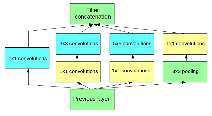
Figure 1: Illustration of Inception module. It was restricted to filter sizes $1\times 1$, $3\times 3$, and $5\times 5$. Subsequently, the outputs were concatenated into a single vector that is the input for the next stage. Adding of an alternative parallel pooling path was found to be beneficial. Applying filters of $1\times 1$ convolution makes possible to reduce the volume before the expensive $3\times 3$ and $5\times 5$ convolutions [31].

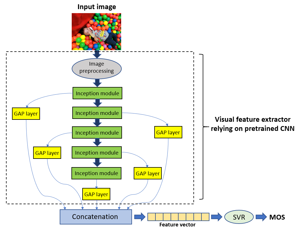
Figure 2: The pipeline of the proposed method. An input image is run through on an ImageNet database pretrained CNN body (GoogLeNet and Inception-V3 are considered in this study) which carries out all its defined operations. Furthermore, global average pooling (GAP) layers are attached to each Inception module to extract resolution independent deep features at different abstraction levels. The feature vectors obtained from the Inception modules are concatenated and an SVR with radial basis function is applied to predict perceptual image quality.

2.1 Pipeline of the proposed method

The pipeline of the proposed framework is depicted in Figure 2. A given input image to be evaluated is run through a pretrained CNN body (GoogLeNet [31] and Inception-V3 [32] are considered in this study) which carries out all its defined operations. Specifically, global average pooling (GAP) layers are attached to the output of each Inception module. Similar to max- or min-pooling layers, GAP layers are applied in CNNs to reduce the spatial dimensions of convolutional layers. However, a GAP layer carries out a more extreme type of dimensional reduction than a max- or min-pooling layer. Namely, an $h\times w\times d$ block is reduced to $1\times 1\times d$. In other words, a GAP layer reduces a feature map to a single value by taking the average of this feature map. By adding GAP layers to each Inception module, we are able to extract resolution independent features at different levels of abstraction. Namely, the feature maps produced by neuroscience models inspired [36] Inception modules have been shown representative for object categories [31], [32] and correlate well with human perceptual quality judgments [39]. The motivation behind the application of GAP layers was the followings. By attaching GAP layers to the Inception modules, we gain an architecture which can be easily generalized to any input image resolution and base CNN architecture. Furthermore, this way the decomposition of the input image into smaller patches can be avoided which means that parameter settings related to the database properties (patch size, number of patches, sampling strategy, etc.) can be ignored. Moreover, some kind of image distortions are not uniformly distributed in the image. These kind of distortions could be better captured in an aspect-ratio and content preserving architecture.

As already mentioned, a feature vector is extracted over each Inception module using a GAP layer. Let $\textbf{f}_{k}$ denote the feature vector extracted from the $k$th Inception module. The input image’s feature vector is obtained by concatenating the respective feature vectors produced by the Inception modules. Formally, we can write $\textbf{F}=\textbf{f}_{1}\oplus\textbf{f}_{2}\oplus...\oplus\textbf{f}_{N}$, where $N$ denotes the number of Inception modules in the base CNN and $\oplus$ stands for the concatenation operator. In Section 3.3, we present a detailed analysis about the effectiveness of different Inception modules’ deep features as a perceptual metric. Furthermore, we point out the prediction performance increase due to the concatenation of deep features extracted from different abstraction levels.

Subsequently, an SVR [40] with radial basis function (RBF) kernel is trained to learn the mapping between feature vectors and corresponding perceptual quality scores.

Moreover, we also applied Gaussian process regression (GPR) with rational quadratic kernel function [41] in Section 3.4.

2.2 Database compilation and transfer learning

Many image quality assessment databases are available online, such as TID2013 [42] or LIVE In the Wild [35], for research purposes. In this study, we selected the recently published KonIQ-10k [33] database to train and test our system, because it is the largest available database containing digital images with authentic distortions. Furthermore, we present a parameter study on KonIQ-10k [33] to find the best design choices. Our best proposal is compared against the state-of-the-art on KonIQ-10k [33] and also on other publicly available databases.

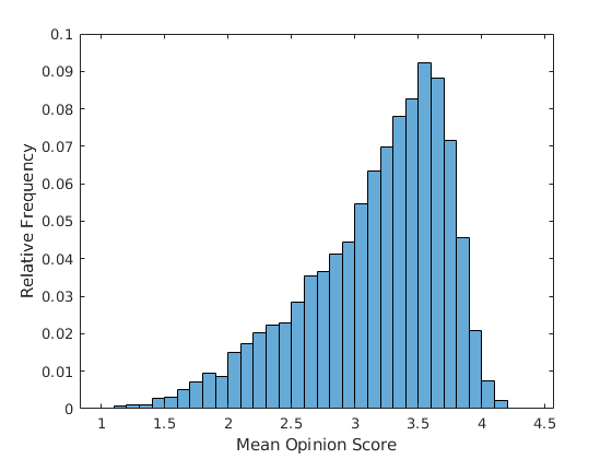
Figure 3: MOS distribution in KonIQ-10k database. It contains 10,073 RGB images with authentic distortions and the corresponding MOS values which are on a scale from 1.0 (worst image quality) to 5.0 (best image quality).

KonIQ-10k [33] consists of 10,073 digital images with the corresponding MOS values. To ensure the fairness of the experimental setup, we selected randomly 6,073 images $(\sim 60\%)$ for training, 2,000 images $(\sim 20\%)$ for validation, and 2,000 images $(\sim 20\%)$ for testing purposes. First, the base CNN was fine-tuned on target database KonIQ-10k [33] using the above-mentioned training and the validation subsets. To this end, regularly the base CNN’s last 1,000-way softmax layer was removed and replaced by a 5-way one in previous methods [18], because the training and validation subsets were reorganized into five classes with respect to the MOS values: class $A$ for excellent image quality $(5.0>MOS\geq 4.2)$, class $B$ for good image quality $(4.2>MOS\geq 3.4)$, class $C$ for fair image quality $(3.4>MOS\geq 2.6)$, class $D$ for poor image quality $(2.6>MOS\geq 1.8)$, and class $E$ for very poor image quality $(1.8>MOS\geq 1.0)$. Subsequently, the base CNN was further train to classify the images into quality categories. Since the MOS distribution in KonIQ-10k [33] is strongly imbalanced (see Figure 3), there would be very little number of images in the class for excellent images. That is why, we took a regression-based approach instead of classification-based approach for fine-tuning. Namely, we removed the base CNN’s last 1,000-way softmax layer and we replaced it by a regression layer containing only one neuron. Since GoogLeNet [31] and Inception-V3 [32] accept images with input size of $224\times 224$ and $299\times 299$, respectively, twenty $224\times 224$-sized or $299\times 299$-sized patches were cropped randomly from each training and validation images. Furthermore, these patches inherit the perceptual quality score of their source images and the fine-tuning is carried out on these patches. Specifically, we trained the base CNN further for regression to predict the images patches MOS values which are inherited from their source images. During fine-tuning Adam optimizer [43] was used, the initial learning rate was set to 0.0001 and divided by 10 when the validation error stopped improving. Further, the batch size was set to 28 and the momentum was 0.9 during fine-tuning.

3 Experimental results and analysis

In this section, we demonstrate our experimental results. First, we give the definition of the evaluation metrics in Section 3.1. Second, we describe the experimental setup and the implementation details in Section 3.2. In Section 3.3, we give a detailed parameter study to find the best design choices of the proposed method using KonIQ-10k [33] database. Subsequently, we carry out a comparison to other state-of-the-art methods using KonIQ-10k [33], KADID-10k [34], and LIVE In the Wild [35] publicly available IQA databases. Finally, we present a so-called cross database test using LIVE In the Wild Image Quality Challenge database [35].

3.1 Evaluation metrics

The performance of NR-IQA algorithms are characterized by the correlation calculated between the ground-truth scores of a benchmark database and the predicted scores. To this end, Pearson’s linear correlation coefficient (PLCC) and Spearman’s rank order correlation coefficient (SROCC) are widely used in the literature [44]. PLCC between datasets $A$ and $B$ is defined as

$$PLCC(A,B)=\frac{\sum_{i=1}^{m}(A_{i}-\bar{A})(B_{i}-\bar{B})}{\sqrt{\sum_{i=1}^{m}(A_{i}-\bar{A})^{2}}\sqrt{\sum_{i=1}^{m}(B_{i}-\bar{B})^{2}}},$$ (1)

where $\bar{A}$ and $\bar{B}$ denote the average of sets $A$ and $B$, and $A_{i}$ and $B_{i}$ denote the $i$th elements of sets $A$ and $B$, respectively. SROCC, it can be expressed as

$$SROCC(A,B)=\frac{\sum_{i=1}^{m}(A_{i}-\hat{A})(B_{i}-\hat{B})}{\sqrt{\sum_{i=1}^{m}(A_{i}-\hat{A})^{2}}\sqrt{\sum_{i=1}^{m}(B_{i}-\hat{B})^{2}}},$$ (2)

where $\hat{A}$ and $\hat{B}$ stand for the middle ranks.

3.2 Experimental setup and implementation details

As already mentioned, a detailed parameter study was carried out on the recently published KonIQ-10k [33], which is the currently largest available IQA database with authentic distortions, to determine the optimal design choices. Subsequently, our best proposal is compared to the state-of-the-art using other publicly available databases as well.

The proposed method was implemented in MATLAB R2019a mainly relying on the functions of the Deep Learning Toolbox (formerly Neural Network Toolbox), Image Processing Toolbox, and Statistics and Machine Learning Toolbox. Thus, the parameter study was also carried out in MATLAB environment. More specifically, it was evaluated by 100 random train-validation-test split of the applied database and we report on the average of the PLCC and SROCC values. As usual in machine learning, $\sim 60\%$ of the images was used for training, $\sim 20\%$ for validation, and $\sim 20\%$ for testing purposes. Moreover, for IQA databases containing artificial distortions the splitting of the database is carried out with respect to the reference images, so no semantic overlapping was between the training, validation, and test sets. Further, the models were trained and tested on a personal computer with 8-core i7-7700K CPU two NVidia Geforce GTX 1080 GPUs.

3.3 Parameter study

First, we conducted experiments to determine which Inception module in GoogLeNet [31] or in Inception-V3 [32] is the most appropriate for visual feature extraction to predict perceptual image quality. Second, we answer the question whether the concatenation of different Inception modules’ feature vectors improves the prediction’s performance or not. Third, we demonstrate that fine-tuning of the base CNN architecture results in significant performance increase. In this parameter study, we used KonIQ-10k database to answer the above mentioned questions and to find the most effective design choices. In the next subsection, our best proposal is used to carry out a comparison to the state-of-the-art using other databases as well.

The results of the parameter study are summarized in Tables 1, 2, 3, and 4. Specifically, Table 1 and 3 contains the results with GoogLeNet [31] and Inception-V3 [32] base architectures without fine-tuning, respectively. On the other hand, Table 2 and 4 summarizes the results when fine-tuning is applied. In these tables, we reported on the average, the median, and the standard deviation of the PLCC and SROCC values obtained after 100 random train-validation-test splits using KonIQ-10k database. Furthermore, we report on the effectiveness of deep features extracted from different Inception modules. Moreover, the tables also contain the prediction performance of the concatenated deep feature vector. From these results, it can be concluded that the deep features extracted from the early Inception modules perform slightly poorer than those of intermediate and last Inception modules. Although most state-of-the-art methods [22], [15], [18] utilize the features of the last CNN layers, it is worth to examine earlier layers as well, because the tables’ data indicate that the middle layers encode those information which are the most powerful for perceptual quality prediction. We can also assert that feature vectors containing both mid-level and high-level deep representations are significantly more efficient than those of containing only one level’s feature representation. Finally, it can be clearly seen that fine-tuning the base CNN architectures also improves the effectiveness of the extracted deep features. On the whole, the deeper Inception-V3 [32] provides more effective features than GoogLeNet [31]. Our best proposal relies on Inception-V3 and concatenates the features of all Inception modules. In the followings, we call this architecture MultiGAP-NRIQA and compare it to other state-of-the-art in the next subsection.

Another contribution of this parameter study may be the followings. It is worth to study the features of different layers separately because the features of intermediate layers may provide a better representation of the given task than high-level features. Furthermore, the proposed feature extraction method may be also superior in other problems where the task is to predict one value only from the image data itself relying on a large enough database.

In our environment (MATLAB R2019a, PC with 8-core i7700K CPU and two NVidia Geforce GTX 1080), the computational times of the proposed MultiGAP-NRIQA method are the followings. The loading of the base CNN and the $1024\times 768$-sized or the $512\times 384$ input image takes about $1.8s$. Furthermore, the feature extraction from multiple Inception modules of Inception-V3 [32] and concatenation takes on average $1.355s$ or $0.976s$ on the GPU, respectively. Furthermore, the SVR regression takes $2.976s$ on average computing on the CPU.

Table 1: Performance comparison of deep features extracted from GoogLeNet’s Inception modules without fine-tuning measured on KonIQ-10k. Average/median $(\pm std)$ values are reported over 100 random train-test splits. The best results are typed by bold.

Layer	Dimension	PLCC	SROCC
inception_3a-output	256	$0.845/0.845(\pm 0.006)$	$0.842/0.841(\pm 0.007)$
inception_3b-output	480	$0.861/0.861(\pm 0.007)$	$0.856/0.858(\pm 0.007)$
inception_4a-output	512	$0.876/0.876(\pm 0.004)$	$0.872/0.872(\pm 0.006)$
inception_4b-output	512	$0.874/0.874(\pm 0.005)$	$0.865/0.864(\pm 0.008)$
inception_4c-output	512	$0.875/0.877(\pm 0.006)$	$0.865/0.865(\pm 0.006)$
inception_4d-output	528	$0.876/0.875(\pm 0.007)$	$0.864/0.864(\pm 0.007)$
inception_4e-output	832	$0.872/0.871(\pm 0.006)$	$0.861/0.862(\pm 0.005)$
inception_5a-output	832	$0.873/0.874(\pm 0.005)$	$0.859/0.860(\pm 0.005)$
inception_5b-output	1024	$0.861/0.861(\pm 0.008)$	$0.851/0.850(\pm 0.008)$
All concatenated	5488	$\textbf{0.889/0.889}(\pm 0.007)$	$\textbf{0.879/0.877}(\pm 0.006)$

Table 2: Performance comparison of deep features extracted from GoogLeNet’s Inception modules with fine-tuning measured on KonIQ-10k. Average/median $(\pm std)$ values are reported over 100 random train-validation-test splits. The best results are typed by bold.

Layer	Dimension	PLCC	SROCC
inception_3a-output	256	$0.850/0.849(\pm 0.007)$	$0.846/0.846(\pm 0.007)$
inception_3b-output	480	$0.866/0.866(\pm 0.006)$	$0.861/0.862(\pm 0.007)$
inception_4a-output	512	$0.881/0.881(\pm 0.005)$	$0.877/0.876(\pm 0.006)$
inception_4b-output	512	$0.877/0.876(\pm 0.005)$	$0.870/0.870(\pm 0.006)$
inception_4c-output	512	$0.879/0.880(\pm 0.005)$	$0.869/0.868(\pm 0.005)$
inception_4d-output	528	$0.880/0.880(\pm 0.006)$	$0.869/0.868(\pm 0.005)$
inception_4e-output	832	$0.877/0.877(\pm 0.005)$	$0.867/0.867(\pm 0.007)$
inception_5a-output	832	$0.878/0.878(\pm 0.007)$	$0.864/0.864(\pm 0.007)$
inception_5b-output	1024	$0.865/0.865(\pm 0.007)$	$0.856/0.856(\pm 0.008)$
All concatenated	5488	$\textbf{0.894/0.894}(\pm 0.006)$	$\textbf{0.884/0.884}(\pm 0.006)$

Table 3: Performance comparison of deep features extracted from Inception-V3’s Inception modules without fine-tuning measured on KonIQ-10k. Average/median $(\pm std)$ values are reported over 100 random train-test splits. The best results are typed by bold.

Layer	Dimension	PLCC	SROCC
mixed0	256	$0.843/0.843(\pm 0.006)$	$0.839/0.839(\pm 0.006)$
mixed1	288	$0.848/0.848(\pm 0.005)$	$0.844/0.844(\pm 0.005)$
mixed2	288	$0.849/0.849(\pm 0.006)$	$0.844/0.844(\pm 0.007)$
mixed3	768	$0.861/0.860(\pm 0.005)$	$0.858/0.855(\pm 0.006)$
mixed4	768	$0.897/0.897(\pm 0.005)$	$0.889/0.889(\pm 0.006)$
mixed5	768	$0.906/0.906(\pm 0.004)$	$0.898/0.898(\pm 0.005)$
mixed6	768	$0.902/0.901(\pm 0.004)$	$0.890/0.891(\pm 0.006)$
mixed7	768	$0.884/0.884(\pm 0.004)$	$0.870/0.870(\pm 0.006)$
mixed8	1280	$0.892/0.891(\pm 0.004)$	$0.879/0.879(\pm 0.006)$
mixed9	2048	$0.871/0.871(\pm 0.005)$	$0.859/0.859(\pm 0.006)$
mixed10	2048	$0.842/0.844(\pm 0.006)$	$0.828/0.829(\pm 0.008)$
All concatenated	10048	$\textbf{0.910/0.911}(\pm 0.005)$	$\textbf{0.901/0.901}(\pm 0.005)$

Table 4: Performance comparison of deep features extracted from Inception-V3’s Inception modules with fine-tuning measured on KonIQ-10k. Average/median $(\pm std)$ values are reported over 100 random train-validation-test splits. The best results are typed by bold.

Layer	Dimension	PLCC	SROCC
mixed0	256	$0.848/0.848(\pm 0.008)$	$0.848/0.848(\pm 0.007)$
mixed1	288	$0.853/0.853(\pm 0.007)$	$0.853/0.853(\pm 0.006)$
mixed2	288	$0.854/0.853(\pm 0.007)$	$0.853/0.853(\pm 0.006)$
mixed3	768	$0.866/0.865(\pm 0.006)$	$0.867/0.867(\pm 0.007)$
mixed4	768	$0.902/0.902(\pm 0.007)$	$0.898/0.897(\pm 0.006)$
mixed5	768	$0.911/0.910(\pm 0.005)$	$0.908/0.908(\pm 0.006)$
mixed6	768	$0.907/0.906(\pm 0.005)$	$0.900/0.900(\pm 0.006)$
mixed7	768	$0.889/0.889(\pm 0.005)$	$0.880/0.880(\pm 0.006)$
mixed8	1280	$0.897/0.897(\pm 0.006)$	$0.888/0.887(\pm 0.008)$
mixed9	2048	$0.876/0.876(\pm 0.005)$	$0.869/0.870(\pm 0.007)$
mixed10	2048	$0.847/0.847(\pm 0.005)$	$0.837/0.836(\pm 0.008)$
All concatenated	10048	$\textbf{0.915/0.914}(\pm 0.005)$	$\textbf{0.911/0.911}(\pm 0.005)$

Table 5: Publicly available IQA databases used in this study. Publicly available IQA databases can be divided into two groups. The first one contains a smaller set of reference images and artificially distorted images are derived from them using different noise types at different intensity levels, while the second one contains images with "natural" degradation without any additional artificial distortions.

Database	Year	Reference images	Test images	Distortion type	Resolution	Subjective score
LIVE In the Wild	2015	-	1,162	authentic	$500\times 500$	MOS (1-5)
KonIQ-10k	2018	-	10,073	authentic	$1024\times 768$	MOS (1-5)
KADID-10k	2019	81	10,125	artificial	$512\times 384$	MOS (1-5)

3.4 Comparison to the state-of-the-art

To compare our proposed method to other state-of-the-art algorithms, we collected ten traditional learning-based NR-IQA metrics ( DIIVINE [2], BLIINDS-II [45], BRISQUE [6], CurveletQA [4], SSEQ [46], GRAD-LOG-CP [47], BMPRI [48], SPF-IQA [49], SCORER [50], ENIQA [51] ), and two opinion-unaware method (NIQE [52], PIQE [53]) whose original source code are available. Moreover, we took the results of two recently published deep learning based NR-IQA algorithms — DeepFL-IQA [54] and MLSP [55] — from their original publication. On the whole, we compared our proposed method — MultiGAP-NRIQA — to 12 other state-of-the-art IQA algorithms or metrics. The results can be seen in Table 6.

To ensure a fair comparison, these traditional and deep methods were trained, tested, and evaluated exactly the same as our proposed method. Specifically, $\sim 60\%$ of the images was used for training, $\sim 20\%$ for validation, and $\sim 20\%$ for testing purposes. If a validation set is not required, the training set contains $\sim 80\%$ of the images. Moreover, for IQA databases containing artificial distortions the splitting of the database is carried out with respect to the reference images, so no semantic overlapping was between the training, validation, and test sets. To compare our method to the state-of-the-art, we report on the average PLCC and SROCC values of 100 random train-validation-test splits of our method and those of other algorithms. As already mentioned, the results are summarized in Table 6. More specifically, this table illustrates the measured average PLCC and SROCC on three large publicly available IQA databases (Table 5 summarizes the major parameters of the IQA databases used in this paper).

From the results, it can be seen that the proposed significantly outperforms the state-of-the-art on KonIQ-10k database. Moreover, only the MultiGAP-NRIQA method is able perform over 0.9 PLCC and SROCC. It can be observed that GPR with rational quadratic kernel function performs better than SVR with Gaussian kernel function. Similarly, the proposed method outperforms the state-of-the-art on LIVE In the Wild IQA database [35] by a large margin. On KADID-10k, DeepFL-IQA [54] provides the best results by a large margin. The proposed MultiGAP-GPR gives the third best results.

Table 6: Comparison of MultiGAP-NRIQA with state-of-the-art NR-IQA and FR-IQA algorithms trained and tested on KonIQ-10k, KADID-10k, and TID2013 databases. The average PLCC and SROCC values are reported measured over 100 random train-validation-test split. The best results are shown in bold and the second best results are typed in italic. The results of DeepFL-IQA [54] and MLSP [55] was measured by the authors of [54].

	KonIQ-10k		KADID-10k		LIVE In the Wild
Method	PLCC	SROCC	PLCC	SROCC	PLCC	SROCC
DIIVINE [2]	0.709	0.692	0.423	0.428	0.602	0.579
BLIINDS-II [45]	0.571	0.575	0.548	0.530	0.450	0.419
BRISQUE [6]	0.702	0.676	0.383	0.386	0.503	0.487
NIQE [52]	-	-	0.273	0.309	-	-
CurveletQA [4]	0.728	0.716	0.473	0.450	0.620	0.611
SSEQ [46]	0.584	0.573	0.453	0.433	0.469	0.429
GRAD-LOG-CP [47]	0.705	0.698	0.585	0.566	0.579	0.557
PIQE [53]	0.206	0.245	0.289	0.237	0.171	0.108
BMPRI [48]	0.636	0.619	0.554	0.530	0.521	0.480
SPF-IQA [49]	0.759	0.740	0.717	0.708	0.592	0.563
SCORER [50]	0.772	0.762	0.855	0.856	0.599	0.590
ENIQA [51]	0.758	0.744	0.634	0.636	0.578	0.554
DeepFL-IQA [54]	0.887	0.877	0.938	0.936	0.842	0.814
MLSP [55]	0.924	0.913	-	-	0.769	0.734
MultiGAP-SVR [56]	0.915	0.911	0.799	0.795	0.841	0.813
MultiGAP-GPR [56]	0.928	0.925	0.820	0.814	0.857	0.826

3.5 Cross database test

To prove the generalization capability of our proposed MultiGAP-NRIQA method, we carry out a so-called cross database test in this subsection. This means that our model was trained on the whole KonIQ-10k [33] database and tested on LIVE In the Wild Image Quality Challenge Database [35]. Moreover, the other learning-based NR-IQA methods were also tested this way. The results are summarized in Table 7. From the results, it can be clearly seen that all learning-based methods performed significantly poorer in the cross database test than in the previous tests. It should be emphasized that our MultiGAP-NRIQA method generalized better than the state-of-the-art traditional or deep learning based algorithms even without fine-tuning. The performance drop occurs owing to the fact that images are treated slightly differently in each publicly available IQA database. For example, in LIVE In The Wild [35] database the images were rescaled. In contrast, the images of KonIQ-10k [33] were cropped from their original counterparts.

Table 7: Cross database test. The learning-based NR-IQA methods were trained on the whole KonIQ-10k database and tested on LIVE In the Wild database. The measured PLCC and SROCC values are reported. The best results are shown in bold and the second best results are typed in italic. The results of DeepFL-IQA [54] was measured by the authors of [54].

	LIVE In The Wild
Method	PLCC	SROCC
BLIINDS-II [3]	0.439	0.401
BRISQUE [6]	0.625	0.604
DIIVINE [2]	0.598	0.592
SSEQ [4]	0.440	0.412
DeepFL-IQA [54]	-	0.704
MLSP [55]	-	-
MultiGAP-NRIQA, RBF SVR (without fine-tuning)	0.841	0.812
MultiGAP-NRIQA, RBF SVR	0.841	0.813
MultiGAP-NRIQA, r.q. GPR (without fine-tuning)	0.856	0.855
MultiGAP-NRIQA, r.q. GPR	0.857	0.856

4 Conclusion

In this paper, we introduced a deep framework for NR-IQA which constructs a feature space relying on multi-level Inception features extracted from pretrained CNNs via GAP layers. Unlike previous deep methods, the proposed approach do not take patches from the input image, but instead treat the image as a whole and extract image resolution independent features. As a result, the proposed approach can be easily generalized to any input image size and CNN base architecture. Unlike previous deep methods, we extract multi-level features from the CNN to incorporate both mid-level and high-level deep representations into the feature vector. Furthermore, we pointed out in a detailed parameter study that mid-level features provide significantly more effective descriptors for NR-IQA. Another important observation was that the feature vector containing both mid-level and high-level representations outperforms all feature vectors containing the representation of one level. We also carried out a comparison to other state-of-the-art methods and our approach outperformed the state-of-the-art on the largest available benchmark IQA databases. Moreover, the results were also confirmed in a cross database test. There are many directions for future research. Specifically, we would like to improve the fine-tuning process in order to transfer quality-aware features more effectively into the base CNN. Another direction of future research could be the generalization of the applied feature extraction method to other CNN architectures, such as residual networks.

References

- [1] Pamela Reinagel and Anthony M Zador. Natural scene statistics at the centre of gaze. Network: Computation in Neural Systems, 10(4):341–350, 1999.
- [2] Anush Krishna Moorthy and Alan Conrad Bovik. Blind image quality assessment: From natural scene statistics to perceptual quality. IEEE transactions on Image Processing, 20(12):3350–3364, 2011.
- [3] Michele A Saad, Alan C Bovik, and Christophe Charrier. Dct statistics model-based blind image quality assessment. In 2011 18th IEEE International Conference on Image Processing, pages 3093–3096. IEEE, 2011.
- [4] Lixiong Liu, Bao Liu, Hua Huang, and Alan Conrad Bovik. No-reference image quality assessment based on spatial and spectral entropies. Signal Processing: Image Communication, 29(8):856–863, 2014.
- [5] Yuming Li, Lai-Man Po, Xuyuan Xu, and Litong Feng. No-reference image quality assessment using statistical characterization in the shearlet domain. Signal Processing: Image Communication, 29(7):748–759, 2014.
- [6] Anish Mittal, Anush Krishna Moorthy, and Alan Conrad Bovik. No-reference image quality assessment in the spatial domain. IEEE Transactions on Image Processing, 21(12):4695–4708, 2012.
- [7] Lihuo He, Dacheng Tao, Xuelong Li, and Xinbo Gao. Sparse representation for blind image quality assessment. In 2012 IEEE Conference on Computer Vision and Pattern Recognition, pages 1146–1153. IEEE, 2012.
- [8] Pedro Garcia Freitas, Luísa Peixoto Da Eira, Samuel Soares Santos, and Mylene Christine Queiroz de Farias. On the application lbp texture descriptors and its variants for no-reference image quality assessment. Journal of Imaging, 4(10):114, 2018.
- [9] Lin Zhang, Lei Zhang, and Alan C Bovik. A feature-enriched completely blind image quality evaluator. IEEE Transactions on Image Processing, 24(8):2579–2591, 2015.
- [10] Jongyoo Kim and Sanghoon Lee. Fully deep blind image quality predictor. IEEE Journal of selected topics in signal processing, 11(1):206–220, 2016.
- [11] Kede Ma, Wentao Liu, Kai Zhang, Zhengfang Duanmu, Zhou Wang, and Wangmeng Zuo. End-to-end blind image quality assessment using deep neural networks. IEEE Transactions on Image Processing, 27(3):1202–1213, 2017.
- [12] Qiang Li and Zhou Wang. Reduced-reference image quality assessment using divisive normalization-based image representation. IEEE journal of selected topics in signal processing, 3(2):202–211, 2009.
- [13] Chunling Fan, Yun Zhang, Liangbing Feng, and Qingshan Jiang. No reference image quality assessment based on multi-expert convolutional neural networks. IEEE Access, 6:8934–8943, 2018.
- [14] Le Kang, Peng Ye, Yi Li, and David Doermann. Convolutional neural networks for no-reference image quality assessment. In Proceedings of the IEEE conference on computer vision and pattern recognition, pages 1733–1740, 2014.
- [15] Sebastian Bosse, Dominique Maniry, Thomas Wiegand, and Wojciech Samek. A deep neural network for image quality assessment. In 2016 IEEE International Conference on Image Processing (ICIP), pages 3773–3777. IEEE, 2016.
- [16] Jie Li, Lian Zou, Jia Yan, Dexiang Deng, Tao Qu, and Guihui Xie. No-reference image quality assessment using prewitt magnitude based on convolutional neural networks. Signal, Image and Video Processing, 10(4):609–616, 2016.
- [17] Jie Li, Jia Yan, Dexiang Deng, Wenxuan Shi, and Songfeng Deng. No-reference image quality assessment based on hybrid model. Signal, Image and Video Processing, 11(6):985–992, 2017.
- [18] Simone Bianco, Luigi Celona, Paolo Napoletano, and Raimondo Schettini. On the use of deep learning for blind image quality assessment. Signal, Image and Video Processing, 12(2):355–362, 2018.
- [19] Alex Krizhevsky, Ilya Sutskever, and Geoffrey E Hinton. Imagenet classification with deep convolutional neural networks. In Advances in neural information processing systems, pages 1097–1105, 2012.
- [20] Fei Gao, Jun Yu, Suguo Zhu, Qingming Huang, and Qi Tian. Blind image quality prediction by exploiting multi-level deep representations. Pattern Recognition, 81:432–442, 2018.
- [21] Weixia Zhang, Kede Ma, Jia Yan, Dexiang Deng, and Zhou Wang. Blind image quality assessment using a deep bilinear convolutional neural network. IEEE Transactions on Circuits and Systems for Video Technology, 2018.
- [22] Lihuo He, Yanzhe Zhong, Wen Lu, and Xinbo Gao. A visual residual perception optimized network for blind image quality assessment. IEEE Access, 7:176087–176098, 2019.
- [23] Weiping Ji, Jinjian Wu, Guangming Shi, Wenfei Wan, and Xuemei Xie. Blind image quality assessment with semantic information. Journal of Visual Communication and Image Representation, 58:195–204, 2019.
- [24] Karen Simonyan and Andrew Zisserman. Very deep convolutional networks for large-scale image recognition. arXiv preprint arXiv:1409.1556, 2014.
- [25] Zhong Zhang, Hong Wang, Shuang Liu, and Tariq S Durrani. Deep activation pooling for blind image quality assessment. Applied Sciences, 8(4):478, 2018.
- [26] Domonkos Varga. No-reference video quality assessment based on the temporal pooling of deep features. Neural Processing Letters, pages 1–14, 2019.
- [27] Forrest N Iandola, Song Han, Matthew W Moskewicz, Khalid Ashraf, William J Dally, and Kurt Keutzer. Squeezenet: Alexnet-level accuracy with 50x fewer parameters and< 0.5 mb model size. arXiv preprint arXiv:1602.07360, 2016.
- [28] Albert Gordo, Jon Almazán, Jerome Revaud, and Diane Larlus. Deep image retrieval: Learning global representations for image search. In European conference on computer vision, pages 241–257. Springer, 2016.
- [29] Omar Alaql and Cheng-Chang Lu. No-reference image quality metric based on multiple deep belief networks. IET Image Processing, 2019.
- [30] Ali Sharif Razavian, Hossein Azizpour, Josephine Sullivan, and Stefan Carlsson. Cnn features off-the-shelf: an astounding baseline for recognition. In Proceedings of the IEEE conference on computer vision and pattern recognition workshops, pages 806–813, 2014.
- [31] Christian Szegedy, Wei Liu, Yangqing Jia, Pierre Sermanet, Scott Reed, Dragomir Anguelov, Dumitru Erhan, Vincent Vanhoucke, and Andrew Rabinovich. Going deeper with convolutions. In Proceedings of the IEEE conference on computer vision and pattern recognition, pages 1–9, 2015.
- [32] Christian Szegedy, Vincent Vanhoucke, Sergey Ioffe, Jon Shlens, and Zbigniew Wojna. Rethinking the inception architecture for computer vision. In Proceedings of the IEEE conference on computer vision and pattern recognition, pages 2818–2826, 2016.
- [33] Hanhe Lin, Vlad Hosu, and Dietmar Saupe. Koniq-10k: Towards an ecologically valid and large-scale iqa database. arXiv preprint arXiv:1803.08489, 2018.
- [34] Hanhe Lin, Vlad Hosu, and Dietmar Saupe. Kadid-10k: A large-scale artificially distorted iqa database. In 2019 Eleventh International Conference on Quality of Multimedia Experience (QoMEX), pages 1–3. IEEE, 2019.
- [35] Deepti Ghadiyaram and Alan C Bovik. Massive online crowdsourced study of subjective and objective picture quality. IEEE Transactions on Image Processing, 25(1):372–387, 2015.
- [36] Thomas Serre, Lior Wolf, Stanley Bileschi, Maximilian Riesenhuber, and Tomaso Poggio. Robust object recognition with cortex-like mechanisms. IEEE Transactions on Pattern Analysis & Machine Intelligence, (3):411–426, 2007.
- [37] Sergey Ioffe and Christian Szegedy. Batch normalization: Accelerating deep network training by reducing internal covariate shift. arXiv preprint arXiv:1502.03167, 2015.
- [38] Ke Gu, Shiqi Wang, Guangtao Zhai, Weisi Lin, Xiaokang Yang, and Wenjun Zhang. Analysis of distortion distribution for pooling in image quality prediction. IEEE Transactions on Broadcasting, 62(2):446–456, 2016.
- [39] Richard Zhang, Phillip Isola, Alexei A Efros, Eli Shechtman, and Oliver Wang. The unreasonable effectiveness of deep features as a perceptual metric. In Proceedings of the IEEE Conference on Computer Vision and Pattern Recognition, pages 586–595, 2018.
- [40] Harris Drucker, Christopher JC Burges, Linda Kaufman, Alex J Smola, and Vladimir Vapnik. Support vector regression machines. In Advances in neural information processing systems, pages 155–161, 1997.
- [41] Carl Edward Rasmussen. Gaussian processes in machine learning. In Summer School on Machine Learning, pages 63–71. Springer, 2003.
- [42] Nikolay Ponomarenko, Lina Jin, Oleg Ieremeiev, Vladimir Lukin, Karen Egiazarian, Jaakko Astola, Benoit Vozel, Kacem Chehdi, Marco Carli, Federica Battisti, et al. Image database tid2013: Peculiarities, results and perspectives. Signal Processing: Image Communication, 30:57–77, 2015.
- [43] Diederik P Kingma and Jimmy Ba. Adam: A method for stochastic optimization. arXiv preprint arXiv:1412.6980, 2014.
- [44] Long Xu, Weisi Lin, and C-C Jay Kuo. Visual quality assessment by machine learning. Springer, 2015.
- [45] Michele A Saad, Alan C Bovik, and Christophe Charrier. Blind image quality assessment: A natural scene statistics approach in the dct domain. IEEE transactions on Image Processing, 21(8):3339–3352, 2012.
- [46] Lixiong Liu, Bao Liu, Hua Huang, and Alan Conrad Bovik. No-reference image quality assessment based on spatial and spectral entropies. Signal Processing: Image Communication, 29(8):856–863, 2014.
- [47] Wufeng Xue, Xuanqin Mou, Lei Zhang, Alan C Bovik, and Xiangchu Feng. Blind image quality assessment using joint statistics of gradient magnitude and laplacian features. IEEE Transactions on Image Processing, 23(11):4850–4862, 2014.
- [48] Xiongkuo Min, Guangtao Zhai, Ke Gu, Yutao Liu, and Xiaokang Yang. Blind image quality estimation via distortion aggravation. IEEE Transactions on Broadcasting, 64(2):508–517, 2018.
- [49] Domonkos Varga. No-reference image quality assessment based on the fusion of statistical and perceptual features. Journal of Imaging, 6(8):75, 2020.
- [50] Mariusz Oszust. Local feature descriptor and derivative filters for blind image quality assessment. IEEE Signal Processing Letters, 26(2):322–326, 2019.
- [51] Xiaoqiao Chen, Qingyi Zhang, Manhui Lin, Guangyi Yang, and Chu He. No-reference color image quality assessment: from entropy to perceptual quality. EURASIP Journal on Image and Video Processing, 2019(1):77, 2019.
- [52] Anish Mittal, Rajiv Soundararajan, and Alan C Bovik. Making a “completely blind” image quality analyzer. IEEE Signal processing letters, 20(3):209–212, 2012.
- [53] N Venkatanath, D Praneeth, Maruthi Chandrasekhar Bh, Sumohana S Channappayya, and Swarup S Medasani. Blind image quality evaluation using perception based features. In 2015 Twenty First National Conference on Communications (NCC), pages 1–6. IEEE, 2015.
- [54] Hanhe Lin, Vlad Hosu, and Dietmar Saupe. Deepfl-iqa: Weak supervision for deep iqa feature learning. arXiv preprint arXiv:2001.08113, 2020.
- [55] Vlad Hosu, Bastian Goldlucke, and Dietmar Saupe. Effective aesthetics prediction with multi-level spatially pooled features. In Proceedings of the IEEE conference on computer vision and pattern recognition, pages 9375–9383, 2019.
- [56] Domonkos Varga. Multi-pooled inception features for no-reference image quality assessment. Applied Sciences, 10(6):2186, 2020.