On the Downlink Performance of RSMA-based UAV Communications

Abstract

The use of unmanned aerial vehicles (UAVs) as base stations (BSs) is envisaged as a key enabler for the fifth generation (5G) and beyond-5G networks. Specifically, aerial base stations (UAV-BS) are expected to provide ubiquitous connectivity and high spectral efficiency. To this end, we present in this correspondence an in-depth look into the integration of rate-splitting multiple access (RSMA) with UAV-BSs and downlink transmissions. A non-convex problem of joint UAV placement, RSMA precoding, and rate splitting, aiming to maximize the weighted sum data rate of users is formulated. Due to its complexity, two sub-problems are investigated, namely the UAV placement and RSMA parameters optimization. The resulting solutions are then combined to propose a novel alternating optimization method. Simulation results illustrate the latter’s efficiency compared to baseline approaches.

I Introduction

There has been a growing interest in unmanned aerial vehicle (UAV) communications, seen as a promising enabler for the fifth generation (5G) and beyond-5G networks [1]–[2]. The deployment of UAVs, driven by the emergence of new applications, such as aerial security inspection, smart agriculture, and aerial delivery, is expected to continue shaping future breakthrough services. UAVs can also serve as aerial base stations (UAV-BS) in order to support ubiquitous connectivity, particularly in rural areas and disaster areas, and high data rates, when deployed in dense areas. In this case, the UAV-BS will be a source of/or experience interference as in conventional cellular networks. Fortunately, such a problem can be addressed by the additional degrees of freedom provided solely by a UAV, i.e., the design of three-dimensional (3D) location and high probability of line-of-sight (LoS) to ground users [3]. Nevertheless, these additional degrees of freedom are not sufficient to provide the best experience to a constantly growing number of ground users. In this respect, downlink multiple access techniques play an important role in realizing the data rate requirements, low latency, and connectivity, without added resources.

Recently, rate-splitting multiple access (RSMA) has been identified as a highly-reliable and spectrum-efficient multiple access scheme, that is capable of outperforming both non-orthogonal multiple access (NOMA) and space division multiple access (SDMA) [4]. RSMA relies on the implementation of a linear precoder at the transmitter and successive interference cancellation (SIC) at the receiver. The process starts by dividing user’s messages into common and private parts at the transmitter. The common parts of (all and/or subsets of) users are combined together and encoded into a single common stream, while the private parts are encoded into distinct private streams. These streams are superimposed and sent over a multiple-input multiple-output (MIMO) channel. Then, each user decodes the first common stream and recovers its own data. At the receiver, the interference from the decoded common stream is removed using the SIC. This is followed by successive decoding of the next common parts (of users’ subsets) and removing them, then by private part decoding, while treating other (common and) private signals as noise.

In [4], Mao et al. showed that RSMA outperforms NOMA and SDMA systems over a wide range of network loads and user deployment scenarios, and that RSMA has a lower-complex receiver design than NOMA. In [5]–[7], it was shown that RSMA provides better energy and spectral efficiency than NOMA and SDMA for several user deployments, and unicast and multicast transmissions. Extensions of these works have been made to other system models, e.g., downlink coordinated multi-point transmission [8], cloud-radio access network (C-RAN) [9], multi-user multi-antenna wireless information and power transfer (SWIPT) [10], hybrid radar-communication system [11], and multi-beam satellite communications [12]. In [13], downlink RSMA was considered from one ground BS to serve several aerial users only, whereas in [14], a UAV-assisted C-RAN system, where RSMA parameters were optimized for joint transmissions from ground and aerial BSs to terrestrial users, was proposed. UAV-BS placement has been previously considered with multiple access, thus the UAV-BS’ altitude and its horizontal location can be either separately or jointly optimized. In [15], the authors investigated joint UAV-BS placement, power and time duration allocations for time-division and frequency-division multiple access (TDMA and FDMA). Xia et al. found in [16] optimal SDMA user grouping and precoding for ground-to-air (user to UAV-BS) communications in order to maximize the achieved sum data rate. Also, UAV-BS placement and NOMA power allocation were separately solved in [17] to maximize the system’s sum rate, whereas an extension to joint NOMA power allocation, user pairing, and UAV-BS placement has been studied in [18].

However, the aforementioned works either focused on simple and well-investigated multiple access techniques such as TDMA, FDMA, SDMA, and single-input-single-output (SISO) NOMA, which are not flexible, and are typically designed for specific scenarios (e.g., single-antenna BS, small number of users, etc.) [15]–[18], or ignored UAV-BS placement optimization when using RSMA on the air-to-ground channels [14]. It is obvious that given the recent research interest into RSMA, the latter has not been sufficiently researched in the context of aerial communications, which motivates us to combine the UAV and RSMA technologies to improve wireless data transmissions to ground users. Specifically, we investigate the joint optimization of UAV placement, RSMA precoding, and rate splitting, in order to maximize the weighted sum rate (WSR) of the downlink communication. Since the optimization problem is non-convex, we propose an alternating optimization (AO) method, where the main problem is divided into two sub-problems, namely UAV placement and RSMA parameters optimization, respectively solved for fixed RSMA configuration (using successive convex optimization) and UAV location (using the weighted minimum mean square error method), then combined into a global algorithm, where the optimization approaches for the sub-problems are iteratively executed.

The rest of the paper is organized as follows. In Section II, the system model is presented and the problem is formulated. Section III details the proposed solutions and discusses their complexity, while Section IV presents the results. Finally, Section V concludes the paper.

Notations: In the remainder of the paper, boldface uppercase and lowercase represent matrices and vectors, respectively. $(\cdot)^{T}$ and $(\cdot)^{H}$ denote the transpose and Hermitian operations respectively. $\mathbb{E}(\cdot)$ is the expectation, $\Re(\cdot)$ is the real part of a complex number, $||\cdot||$ is the Euclidean norm, $|\cdot|$ is the absolute value, 0 is the zero matrix, I is the identity matrix, $\mathbbm{1}_{a\times b}$ is $a\times b$ all-ones matrix, and tr$(\cdot)$ is the trace of a matrix.

II System Model and Problem Formulation

II-A System Model

We consider a downlink one layer rate-splitting (RS) transmission where a hovering UAV-BS, equipped with $N_{t}$ antennas, is communicating with $K$ single-antenna users, using a dedicated frequency band. At the UAV side, the distinct messages of all users denoted by $M_{k}$ ($k=1,2,...,K$) are initially divided into common and private parts as $M_{k}=\{M_{k}^{p},M_{k}^{c}\}$. Then, all common messages from all users are encoded together into a single stream $s_{0}$, for the purpose of reducing interference. This stream $s_{0}$ will be eventually decoded by all users. Meanwhile, the private message of each user is encoded into a separate private stream $s_{k}$ ($k=1,2,...,K$) that will be decoded by the corresponding user only. Hence, the vector of the $K+1$ streams to be transmitted is denoted by $\textbf{s}=[s_{0},s_{1},s_{2},...,s_{K}]^{T}$. It is to be noted that a generalized RS model can be obtained by following the same steps as in [4]. For the sake of simplicity, we keep such design out of the scope of this paper, and focus on the simplified version of one common signal only. In order to reduce multi-user interference, precoding $\textbf{P}=[\textbf{p}_{0},\textbf{p}_{1},\textbf{p}_{2},...,\textbf{p}_{K}]_{N_{t}\times(K+1)}$ is utilized to give the streams appropriate weights at each transmitting antenna. Finally, signals are superimposed and broadcast as $\textbf{x}=[x_{1},\ldots,x_{N_{t}}]^{T}=\textbf{P}\;\textbf{s}$. Hence, the received signal at user $k$ can be written as

$$\small y_{k}=\mathbf{h}_{k}^{H}\mathbf{P}\mathbf{s}+n_{k},\qquad\forall k=\{1,\ldots,K\},$$ (1)

where $n_{k}$ is the circularly symmetric complex additive white Gaussian noise (AWGN) with zero-mean and variance $\sigma^{2}$, and $\mathbf{h}_{k}=[h_{k}^{1},\ldots,h_{k}^{N_{t}}]^{T}\in{\mathbb{R}^{N_{t}\times 1}}$ is the air-to-ground channel from the UAV to user $k$. We assume that the air-to-ground communication channels are dominated by line-of-sight (LoS) links, thus, the channel coefficient $h_{k}^{j}$ ($j=1,\ldots,N_{t}$) follows the free-space path loss model expressed by [19]

$$\small h_{k}^{j}={{d_{k}}^{-{{\frac{\beta}{2}}}}},\qquad\forall j=\{1,\ldots,N_{t}\},$$ (2)

where $d_{k}=||\textbf{q}-\textbf{q}_{k}||_{2}$ is the distance between the UAV and user $k$, $\textbf{q}=[x,y,z]$ and $\textbf{q}_{k}=[x_{k},y_{k},z_{k}]$ are the UAV and user $k$ 3D locations, respectively, and $\beta=2$ is the free space path-loss factor [19]. Following [7, 14], channels are assumed perfectly known at the transmitter and receivers. Also, we assume that $\mathbb{E}\{\textbf{s}\textbf{s}^{H}\}=\textbf{{I}}$ and that the transmit power budget at the UAV is constrained by $\text{tr}(\textbf{P}\textbf{P}^{H})\leq P_{t}$, where $P_{t}$ is the UAV’s maximal transmit power.

The decoding procedure at the $k^{th}$ user is described as follows. Since the common stream $s_{c}$ is allocated the highest power, it will be decoded first by treating the rest of the received signal as noise. Then, the $k^{th}$ user will extract its intended information from the common stream. In order to improve the detection of the private stream, each user will apply SIC to remove the effect of the common stream. Finally, the $k^{th}$ user will decode its intended private stream $s_{k}$ by considering the rest of the other users’ private streams as noise. Hence, the received signal-to-interference-plus-noise ratios (SINRs) of the common and private streams $s_{0}$ and $s_{k}$ at $k^{th}$ user, can be given by

$$\small\gamma_{k}^{c}=\frac{|\mathbf{h}_{k}^{H}\mathbf{p}_{0}|^{2}}{\sum\limits_{i=1}^{K}|\mathbf{h}_{k}^{H}\mathbf{p}_{i}|^{2}+\sigma^{2}}=\frac{d_{k}^{-2}|\mathbbm{1}\mathbf{p}_{0}|^{2}}{\sum\limits_{i=1}^{K}d_{k}^{-2}|\mathbbm{1}\mathbf{p}_{i}|^{2}|+\sigma^{2}},\;\forall k\in\{1,\ldots,K\}$$ (3)

and

$$\small\gamma_{k}^{{k}}=\frac{|\mathbf{h}_{k}^{H}\mathbf{p}_{k}|^{2}}{\sum\limits_{\begin{subarray}{c}i=1\\ i\neq k\end{subarray}}^{K}|\mathbf{h}_{k}^{H}\mathbf{p}_{i}|^{2}+\sigma^{2}}=\frac{d_{k}^{-2}|\mathbbm{1}\mathbf{p}_{k}|^{2}}{\sum\limits_{\begin{subarray}{c}i=1\\ i\neq k\end{subarray}}^{K}d_{k}^{-2}|\mathbbm{1}\mathbf{p}_{i}|^{2}|+\sigma^{2}},\;\forall k\in\{1,\ldots,K\},$$ (4)

where $\mathbbm{1}=\mathbbm{1}_{1\times N_{t}}$. Let $R_{k}^{j}=B\;\text{log}_{2}\left(1+\gamma_{k}^{j}\right)$ be the data rate corresponding to the received SINR $\gamma_{k}^{j}$, $\forall k\in\{1,2,...,K\}$, $\forall j\in\{c,1,2,...,K\}$, where $B$ is the used bandwidth. Then, in order to ensure that the common message $s_{0}$ is successfully decoded by all users, the achievable common data rate should not exceed $R_{c}=\text{min}\left\{R_{1}^{c},R_{2}^{c},...,R_{K}^{c}\right\}$. We denote by $R_{k,\rm{com}}$ the portion of the common rate allocated to user $k$. Then, we have $R_{c}=\sum\limits_{k=1}^{K}R_{k,\rm{com}}$. Finally, the overall achievable data rate of user $k$ can be expressed as

$$R_{k,\rm{ov}}=R_{k,\rm{com}}+R_{k}^{{k}}.\;\;\forall k\in\{1,...,K\}.$$ (5)

II-B Problem Formulation

In this paper, we jointly optimize the precoding matrix P, the common rate vector $\textbf{r}=[R_{1,\rm{com}},R_{2,\rm{com}},...,R_{K,\rm{com}}]$, and the UAV 3D location, with the aim of maximizing the weighted sum of overall achievable data rates (WSR), defined as $R_{\rm{ov}}=\sum_{k=1}^{K}w_{k}R_{k,\rm{ov}}$, where $w_{k}$ ($k=1,\ldots,K$) is the weight reflecting $k$th user traffic priority. For a given weight vector $\textbf{w}=[w_{1},\ldots,w_{K}]$, the optimization problem can be formulated as follows:

$$\max_{\mathbf{P},\mathbf{r},\mathbf{q}} \quad{\text{WSR}=R_{\rm{ov}}=\sum_{k=1}^{K}w_{k}R_{k,\rm{ov}}}$$ (P1)

s.t. $$\sum_{k=1}^{K}R_{k,\rm{com}}\leq R_{c}$$ (P1.a)

$$R_{k,\rm{ov}}\geq R_{k,\rm{th}},\;\forall k\in\{1,\ldots,K\}$$ (P1.b)

$$\text{tr}(\mathbf{P}\mathbf{P}^{H})\leq P_{t}$$ (P1.c)

$$\mathbf{r}\geq\mathbf{0}$$ (P1.d)

$${x_{\rm{min}}\leq x\leq x_{\rm{max}},y_{\rm{min}}\leq y\leq y_{\rm{max}},z_{\rm{min}}\leq z\leq z_{\rm{max}}},$$ (P1.e)

where $R_{k,\rm{th}}$ is the minimum required rate at user $k$ to ensure respect of QoS, and ($x_{\min}$,$x_{\max},y_{\min}$,$y_{\max}$,$z_{\min}$,$z_{\max}$) are the minimum and maximum 3D placement coordinates. Problem (P1) is highly non-convex. In fact, for a given UAV location, the problem reduces to WSR maximization by optimizing the precoding matrix and rate-splitting for one layer RSMA, as in [20]. It has been shown that the latter problem is non-convex and non-trivial due to the appearance of the precoder weights in the denominator of the SINR equations [21]. Thus, by reduction, we deduce that (P1) is non-convex.

III Proposed Solution

In order to solve the joint problem in (P1), we propose a low-complexity iterative algorithm, based on the alternate optimization of the UAV placement and RSMA parameters.

III-A UAV Placement Optimization

Assuming that P and r are given, then (P1) reduces to the following UAV placement problem (P2):

$$\max_{\mathbf{q},\boldsymbol{\eta}} \quad{{\sum_{k=1}^{K}w_{k}\;\eta_{k}}}$$ (P2)

$${\eta_{k}\leq\text{log}_{2}\left(1+{|\mathbbm{1}\mathbf{p}_{k}|^{2}}/\left({\sum\limits_{\begin{subarray}{c}i=1\\ i\neq k\end{subarray}}^{K}|\mathbbm{1}\mathbf{p}_{i}|^{2}+\sigma^{2}||{\mathbf{q}-\mathbf{q}_{k}}||_{2}^{2}}\right)\right),\;\forall k,}$$ (P2.a)

$${||{\mathbf{q}-\mathbf{q}_{k}}||_{2}^{2}\leq{\frac{1}{\sigma^{2}}\left(\frac{|\mathbbm{1}\mathbf{p}_{k}|^{2}}{\Lambda_{k}}-\sum_{\begin{subarray}{c}i=1\\ i\neq k\end{subarray}}^{K}|\mathbbm{1}\mathbf{p}_{i}|^{2}\right),\;\forall k},}$$ (P2.b)

$${x_{\rm{min}}\leq x\leq x_{\rm{max}},y_{\rm{min}}\leq y\leq y_{\rm{max}},z_{\rm{min}}\leq z\leq z_{\rm{max}},}$$ (P2.c)

where $\eta_{k}\geq 0$ is a SINR slack variable, which respects constraint (P2.a), $\Lambda_{k}=2^{A_{k}/B}-1$, $A_{k}=R_{k,\rm{th}}-R_{k,\rm{com}}$, and constraint (P2.b) is equivalent to (P1.b). Problem (P2) is non-convex due to the non-convexity of constraint (P2.a) with respect to q. To handle this issue, we opt for successive convex approximation (SCA) technique, where in each iteration, the right-hand side of (P2.a) is replaced by its concave lower bound at a given UAV location denoted by $\textbf{q}^{(l)}$, with $l$ designating the $l^{th}$ iteration. Recalling that any convex function is globally lower-bounded by its first-order Taylor expansion at any point, and by following a similar approach as in [22], (P2) can be approximated in iteration $l$ by

$$\max_{\mathbf{q},\boldsymbol{\eta}} \quad{\sum_{k=1}^{K}w_{k}\eta_{k}}$$ (P3)

$$\eta_{k}\leq R_{k}^{k,(l)},\;\forall k\in\{1,\ldots,K\}$$ (P3.a)

$${\text{(\ref{c2_2})}-\text{(\ref{c2_4})},}$$ (P3.b)

where $R_{k}^{k,(l)}$ is the lower bound of the private signal data rate at the $l^{th}$ iteration, expressed by

$$\small R_{k}^{k,(l)}=-A_{k}^{(l)}\left(d_{k}^{2}-\left(d_{k}^{(l)}\right)^{2}\right)+B_{k}^{(l)},$$ (10)

with

$$\small A_{k}^{(l)}=\frac{\log_{2}(e)|\mathbbm{1}\mathbf{p}_{k}|^{2}}{\left(\sum\limits_{\begin{subarray}{c}i=1\\ i\neq k\end{subarray}}^{K}|\mathbbm{1}\mathbf{p}_{i}|^{2}+\sigma^{2}\left(d_{k}^{(l)}\right)^{2}\right)\left(\sum\limits_{i=1}^{K}|\mathbbm{1}\mathbf{p}_{i}|^{2}+\sigma^{2}\left(d_{k}^{(l)}\right)^{2}\right)},$$ (11)

$$\small B_{k}^{(l)}=\log_{2}\left(1+{|\mathbbm{1}\mathbf{p}_{k}|^{2}}/\left({\sum\limits_{\begin{subarray}{c}i=1\\ i\neq k\end{subarray}}^{K}|\mathbbm{1}\mathbf{p}_{i}|^{2}+\sigma^{2}\left(d_{k}^{(l)}\right)^{2}}\right)\right),$$ (12)

and $d_{k}^{(l)}=||\mathbf{q}^{(l)}-\mathbf{q}_{k}||_{2}$, $\forall k=1,\ldots,K$. Hence, problem (P3) is a convex quadratically constrained quadratic programming problem, which can be solved efficiently using existing software tools such as CVX [23].

III-B RSMA Precoding and Rate-Splitting

Given a UAV location q, problem (P1) can be reduced to

$$\small\max_{\mathbf{P},\mathbf{r}} \quad{\text{WSR}=R_{\rm{ov}}}$$ (P4)

s.t. $$\text{(\ref{c1})--(\ref{c4})}.$$ (P4.a)

Similar to (P1), problem (P4) is also non-convex. To solve it, we adopt the same weighted minimum mean square error (WMMSE) approach as in [4, 20], where (P4) is transformed into an augmented weighted mean square error (AWMSE) problem (P5) as follows. First, any user $k$ ($k=1,\ldots,K$) detects and estimates $s_{0}$ as $\hat{s}_{0}=e_{k}^{0}y_{k}$, where $e_{k}^{0}$ is the equalizer. After successfully decoding $s_{0}$ and subtracting it from the received signal, $s_{k}$ can be detected and estimated as

$$\small\hat{s}_{k}=e_{k}^{k}(y_{k}-\textbf{h}_{k}^{H}\textbf{p}_{0}s_{0})=e_{k}^{k}(y_{k}-d_{k}^{-1}\mathbbm{1}\textbf{p}_{0}s_{0}).$$ (14)

The mean square error (MSE) of each stream can be defined as $\varepsilon_{k}=\mathbb{E}\{|s_{k}-\hat{s}_{k}|^{2}\}$, calculated as

$$\small\varepsilon_{k}^{0}=|e_{k}^{0}|^{2}T_{k}^{0}-2\Re(e_{k}^{0}d_{k}^{-1}\mathbbm{1}\textbf{p}_{0})+1$$ (15)

and

$$\small\varepsilon_{k}^{k}=|e_{k}^{k}|^{2}T_{k}^{k}-2\Re(e_{k}^{k}d_{k}^{-1}\mathbbm{1}\textbf{p}_{u})+1,$$ (16)

where $T_{k}^{0}=\sum_{i=0}^{K}d_{k}^{-2}|\mathbbm{1}\textbf{p}_{i}|^{2}+\sigma^{2}$ and $T_{k}^{k}=T_{k}^{0}-|d_{k}^{-1}\mathbbm{1}\textbf{p}_{0}|^{2}+\sigma^{2}$ are the received power at user $k$ ($k=1,\ldots,K$) to decode signals $s_{0}$ and $s_{k}$, respectively. The optimal MMSE equalizers can then be written as [20]

$$\small(e_{k}^{0})^{\rm MMSE}=\textbf{p}_{0}^{H}\textbf{h}_{k}(T_{k}^{0})^{-1}\;\text{and}\;(e_{k}^{k})^{\rm MMSE}=\textbf{p}_{k}^{H}\textbf{h}_{k}(T_{k}^{k})^{-1}.$$ (17)

By substituting (17) into (15)–(16), the MMSEs are written as

$$\small(\varepsilon_{k}^{0})^{\rm MMSE}=\min_{f_{k}^{0}}\varepsilon_{k}^{0}=(T_{k}^{0})^{-1}I_{k}^{0}\;\text{and}\;(\varepsilon_{k}^{k})^{\rm MMSE}=(T_{k}^{k})^{-1}I_{k}^{k},$$ (18)

where $I_{k}^{0}=T_{k}^{0}-d_{k}^{-2}|\mathbbm{1}\textbf{p}_{0}|^{2}$ and $I_{k}^{k}=T_{k}^{k}-d_{k}^{-2}|\mathbbm{1}\textbf{p}_{k}|^{2}$ are the interference terms when decoding $s_{0}$ and $s_{k}$, respectively. Subsequently, the SINRs can be expressed by

$$\small\gamma_{k}^{0}=1/((\varepsilon_{k}^{0})^{\rm MMSE})-1\;\text{and}\;\gamma_{k}^{k}=1/((\varepsilon_{k}^{k})^{\rm MMSE})-1,$$ (19)

and the common and private data rates by

$$\small R_{k}^{0}=-\log_{2}\left((\varepsilon_{k}^{0})^{\rm MMSE}\right)\;\text{and}\;R_{k}^{k}=-\log_{2}\left((\varepsilon_{k}^{k})^{\rm MMSE}\right),$$ (20)

respectively. Consequently, the AWMSEs are given by

$$\small\zeta_{k}^{0}=u_{k}^{0}\varepsilon_{k}^{0}-\log_{2}\left(u_{k}^{0}\right)\;\text{and}\;\zeta_{k}^{k}=u_{k}^{k}\varepsilon_{k}^{k}-\log_{2}\left(u_{k}^{k}\right),$$ (21)

where $u_{k}^{j}>0$ ($j=0,k$), are weights associated with the MSEs of user $k$ ($k=1,\ldots,K$). By setting the optimization variables as the equalizers and weights, the relation data rates–WMMSEs can be given as [20]

$$\small(\zeta_{k}^{0})^{\rm MMSE}=\min_{\mu_{k}^{0},f_{k}^{0}}\zeta_{k}^{0}=1-R_{k}^{0}\;\text{and}\;(\zeta_{k}^{k})^{\rm MMSE}=\min_{\mu_{k}^{k},f_{k}^{k}}\zeta_{k}^{k}=1-R_{k}^{k}.$$ (22)

By substituting (22) into (21), and after some manipulations

$$\small(u_{k}^{0})^{*}=\left((\varepsilon_{k}^{0})^{\rm MMSE}\right)^{-1}\;\text{and}\;(u_{k}^{k})^{*}=\left((\varepsilon_{k}^{k})^{\rm MMSE}\right)^{-1}.$$ (23)

Motivated by the data rates-WMMSE relations in (22), the optimization problem (P4) can be reformulated as

$$\small\min_{\mathbf{P},\mathbf{v},\mathbf{u},\mathbf{e}} \quad\sum_{u=1}^{K}w_{k}\zeta_{k}^{\rm tot}$$ (P5)

s.t. $$\sum_{k=1}^{K}v_{k}^{0}+1\geq\zeta_{0},$$ (P5.a)

$$\zeta_{k}^{\rm tot}\leq 1-R_{k,\rm th},\;\forall k\in\{1,\ldots,K\}$$ (P5.b)

$$\text{tr}(\mathbf{P}\mathbf{P}^{H})\leq P_{t}$$ (P5.c)

$$\mathbf{v}\leq\mathbf{0}$$ (P5.d)

where $\textbf{v}=[v_{1}^{0},\ldots,v_{K}^{0}]=-\textbf{r}$, $\textbf{u}=[u_{1}^{0},\ldots,u_{K}^{0},u_{1}^{1},\ldots,u_{K}^{K}]$, $\textbf{e}=[e_{1}^{0},\ldots,e_{K}^{0},e_{1}^{1},\ldots,e_{K}^{K}]$, $\zeta_{k}^{\rm tot}=v_{k}^{0}+\zeta_{k}^{k}$ ($k=1,\ldots,K$), and $\zeta_{0}=\max\{\zeta_{1}^{0},\ldots,\zeta_{K}^{0}\}$. When minimizing the objective in (P5) for u and e (fixed P and v), the optimal MMSE ($\textbf{u}^{\rm MMSE}$,$\textbf{e}^{\rm MMSE}$) is obtained according to (17) and (23). The obtained values satisfy the Karush Kuhn Tucker (KKT) optimality conditions in (P5) for P. Thus, given (22) and the common rate transformation $\textbf{v}=-\textbf{r}$, (P5) can be transformed into (P4). Similarly, for any solution ($\textbf{P}^{*}$,$\textbf{v}^{*}$,$\textbf{u}^{*}$,$\textbf{e}^{*}$) that satisfies the KKT conditions in (P5), the solution ($\textbf{r}^{*}=-\textbf{v}^{*}$,$\textbf{P}^{*}$) satisfies the KKT conditions in (P4). Consequently, (P4) can be transformed into (P5). However, (P5) is also non-convex for joint parameters optimization. To solve it, Mao et al. proposed in [4] to adopt an AO method as follows. In the $l^{th}$ iteration of the AO algorithm, the equalizers and weights are updated using the precoders obtained in the $(l-1)^{th}$ iteration, i.e.,

$$(\textbf{u},\textbf{e})=(\textbf{u}^{\rm MMSE}(\textbf{P}[l-1]),\textbf{e}^{\rm MMSE}(\textbf{P}[l-1])).$$

Then, (v,P) is updated by solving (P5) for ($\mathbf{u}$,$\mathbf{e}$). Hence, (u, e) and (v, P) are iteratively updated until convergence of the WSR. The details of the procedure are presented in Algorithm 1, where $[l]$ is the iteration index, $\mathbf{u}$ is the stream’s weight vector, $\mathbf{e}$ is the equalizer vector, $\mathbf{v}$ is the transformation of $\mathbf{r}$, and $\varepsilon\ll 1$ is the convergence condition [4].

Algorithm 1 RSMA Precoding-Rate Splitting Algorithm

1:Initialize $l\xleftarrow{}0$, $\mathbf{P}^{(l)}$, ${R}_{\rm{ov}}^{(l)}$

2:repeat

3:    Set $l\xleftarrow{}l+1$; $\mathbf{P}^{(l-1)}\xleftarrow{}\mathbf{P}$

4:    Set $\mathbf{u}\xleftarrow{}\mathbf{u}^{\rm{MMSE}}(\mathbf{P}^{(l-1)})$; $\mathbf{e}\xleftarrow{}\mathbf{e}^{\rm{MMSE}}(\mathbf{P}^{(l-1)})$

5:    Solve (P5) for updated ($\mathbf{u},\mathbf{e}$), then update ($\mathbf{P}$, $\mathbf{v}$)

6:until $|{R}_{\rm{ov}}^{(l)}-{R}_{\rm{ov}}^{(l-1)}|\leq\varepsilon$

7:Return ($\textbf{P},-\textbf{v}$) and $R_{\rm{ov}}^{(l)}$ % since $\textbf{v}=-\textbf{r}$ [4]

III-C Joint UAV Placement and RSMA Parameters Optimization

Given the solutions to the independent UAV placement and RSMA precoding-rate splitting sub-problems, we propose here a joint optimization algorithm that solves (P1) iteratively. Indeed, our solution, shown in Algorithm 2, alternates between solving (P2) for fixed P and R and solving (P4) for a fixed UAV location. This procedure continues until convergence of the WSR, i.e., the difference between WSR performances of the current and previous iterations is below $\varepsilon$.

Algorithm 2 Joint UAV Placement and RSMA Parameters Optimization Algorithm

1:Initialize $l\xleftarrow{}0$, ($\textbf{q}^{(l)},\textbf{P}^{(l)},\textbf{u}^{(l)},\textbf{e}^{(l)},\textbf{v}^{(l)},{R}_{\rm ov}^{(l)}$)

2:Set $l\xleftarrow{}l+1$

3:repeat

4:    

Given ($\textbf{P}^{(l-1)},\textbf{u}^{(l-1)},\textbf{e}^{(l-1)},\textbf{v}^{(l-1)}$), solve (P3) using the SCA method and get the solution $\textbf{q}^{(l)}$

5:    

Given $\textbf{q}^{(l)}$, solve (P4) using the AO method in Algorithm 1 and get the solution ($\textbf{P}^{(l)},\textbf{u}^{(l)},\textbf{e}^{(l)},\textbf{v}^{(l)},{R}_{\rm ov}^{(l)}$)

6:    Set $l\xleftarrow{}l+1$

7:until $|{R}_{\rm{ov}}^{(l-1)}-{R}_{\rm{ov}}^{(l-2)}|\leq\varepsilon$

8:Return $(\textbf{q}^{*},\textbf{P}^{*},\textbf{r}^{*},R_{\rm{ov}}^{*})$

III-D Complexity Analysis

In Algorithm 2, the complexity of solving problem (P1) resides mainly in the complexity of solving problems (P2) and (P4). The UAV placement problem (P2) is solved using the SCA approach. Since we have $(2K+3)$ constraints in (P3), the required number of iterations by SCA is $\mathcal{O}\left(\sqrt{2K+3}\log_{2}(1/\varepsilon)\right)$, where $\varepsilon$ is the accuracy of SCA [23]. At each iteration, (P3) is solved with complexity $\mathcal{O}\left(Y_{1}^{2}Y_{2}\right)$, where $Y_{1}=K+3$ and $Y_{2}=2K+3$ are the number of variables and constraints, respectively [24]. Thus, the overall SCA complexity to solve (P2) is $\mathcal{O}\left(K^{1.5}\log_{2}\left(1/\varepsilon\right)\right)$. As presented in Algorithm 1, (P5) can be solved using alternating optimization (AO). For each iteration in Algorithm 1, the complexity is dominated by step 5, which solves (P5) using the interior-point method. Given $(N_{t}+1)K$ variables, step 5 has complexity $\mathcal{O}\left((N_{t}K)^{3}\right)$ [25], and subsequently, the complexity of Algorithm 1 is $\mathcal{O}\left(Y_{3}K^{3}N_{t}^{3}\right)$, where $Y_{3}$ is the number of iterations in Algorithm 1. Finally, the complexity of Algorithm 2 that solves problem (P1) is $\mathcal{O}(Y_{4}K^{1.5}\log_{2}(1/\varepsilon)+Y_{4}Y_{3}K^{3}N_{t}^{3})$, where $Y_{4}$ is the number of iterations in Algorithm 2.

IV Numerical Results

We consider an RSMA-based UAV system, where one $N_{t}$-antenna UAV-BS is deployed to serve randomly located $K$ users in an area of $300\times 300$ m². For the sake of simplicity, we assume that users are on the ground, i.e., $z_{k}=0$, $\forall k\in\{1,\ldots,K\}$, the noise power $\sigma^{2}=1$, $\textbf{w}=[1,\ldots,1]$ (corresponds to calculating the sum rate), the bandwidth $B=20$ MHz, and the data rate threshold $R_{k,\rm{th}}=0$ Mbps.

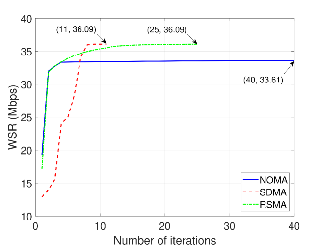
Figure 1: WSR vs. number of iterations ($K=2$, $N_{t}=2$, SNR$=\frac{P_{t}}{\sigma^{2}}=20$ dB, $z_{\min}=80$ m, $z_{\max}=120$ m).

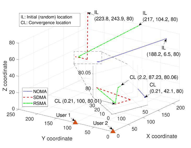
Figure 2: Convergence of the UAV-BS to the best location ($K=2$, $N_{t}=2$, SNR$=\frac{P_{t}}{\sigma^{2}}=20$ dB, $z_{\min}=80$ m, $z_{\max}=120$ m).

In Figs. 1–2, we illustrate the iteration convergence behavior of Algorithm 2 in terms of WSR and UAV-BS location respectively. In Fig. 1, we see that RSMA and SDMA achieve the best performance, with SDMA converging the fastest. Indeed, since the system is underloaded, the number of antennas $N_{t}$ is sufficient to efficiently handle the multi-user interference. RSMA converges slower than SDMA since it requires more time to adapt its behavior to act like it. Finally, NOMA presents the worst performance since it does not mitigate as efficiently the multi-user interference.

From Fig. 2, we see that the UAV-BS converges to a different location, depending on the used multiple access technique. Indeed, the convergence locations are either on or are very close to the Y-Z plan (where the users are located), and are almost at the same minimum allowed altitude $z_{\min}$ [26]. Nevertheless, RSMA and SDMA favor locations close to one of the users, while the UAV-BS for NOMA is closer to the middle point between them. In fact, RSMA and SDMA look for UAV-BS locations that provide non-degraded channels, whereas NOMA prefers a location with degraded air-to-ground channels to perform best [4, 27].

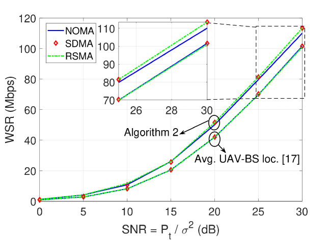
Figure 3: WSR vs. SNR$=\frac{P_{t}}{\sigma^{2}}$ ($K=4$, $N_{t}=4$, $z_{\min}=80$m, $z_{\max}=120$m).

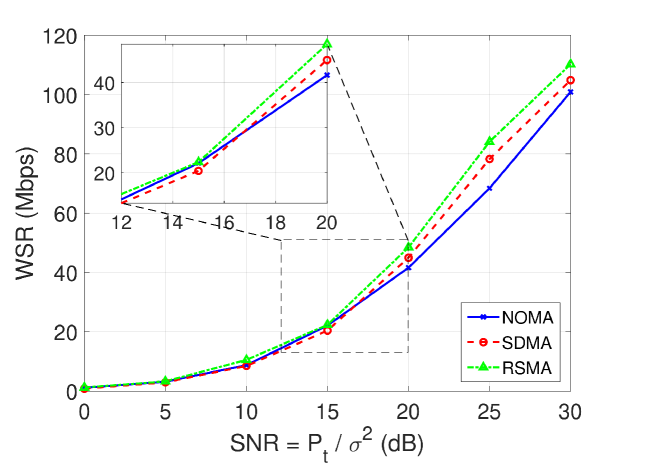
Figure 4: WSR vs. SNR$=\frac{P_{t}}{\sigma^{2}}$ ($K=4$, $N_{t}=4$, $z_{\min}=80$m, $z_{\max}=120$m).

Fig. 3 illustrates the WSR performance as a function of SNR for a system of $K=4$ users, with their locations selected as $\textbf{q}_{1}=[0,0,0]$, $\textbf{q}_{2}=[0,100,0]$, $\textbf{q}_{3}=[150,150,0]$, and $\textbf{q}_{4}=[200,50,0]$. The proposed Algorithm 2 is compared to a baseline method, called “Avg. UAV-BS loc.”, which separates the multiple access problem from the UAV-BS placement one, as in [17]. Subsequently, we notice that Algorithm 2 outperforms “Avg. UAV-BS loc.” for any multiple access scheme. Moreover, RSMA is improved over SDMA and NOMA using our approach, whereas the same performance is achieved by the latter techniques for “Avg. UAV-BS loc.”. This is due for the optimized UAV-BS locations using Algorithm 2.

Finally, in order to explicitly emphasize the superiority of RSMA over SDMA and NOMA, we adopt for Fig. 4 the same scenario as Fig. 3 but with a Rician channel model as follows. The channel coefficient $h_{k}^{j}$, ($j=1$ to $N_{t}$), follows a Rician distribution with parameter $\alpha(\theta_{k})$ [28] and is expressed by

$$\small h_{k}^{j}={d_{k}^{-{{\frac{\beta}{2}}}}}{g_{k}^{j}(\alpha(\theta_{k}))},\qquad\forall j=1,\ldots,N_{t},$$ (25)

where $\theta_{k}$ is the elevation angle between user $k$ and the UAV, $g_{k}^{j}(\alpha(\theta_{k}))$ is the small-scale fading, which follows a Rician distribution with K-factor $\alpha(\theta_{k})$ and $\mathbb{E}\left\{||g_{k}^{j}||^{2}\right\}=1$. Also, $\alpha(\theta_{k})=a_{1}e^{\theta_{k}b_{1}}$, and ($a_{1},b_{1}$)=(10^0.5, 10^1.5) are constants [28]. For the sake of simplicity, we solve (P4) for the generated Rician channel coefficients, while (P3) is solved based on the large-scale channels only. The Rician small-scale coefficients are selected such that the resulting channels are neither aligned, nor orthogonal [4]. According to Fig. 4, RSMA is superior to NOMA and SDMA. Indeed, rate-splitting and precoding, combined to adequate UAV-BS placement, provides non-degraded channels that enable significant WSR gains. At low SNR, NOMA performs slightly better than SDMA due to the limited power, which performs well over degraded channels. In contrast, SDMA outperforms NOMA at high SNR due to its capability to mitigate interference efficiently.

V Conclusion

In this paper, we presented an in-depth look into the integration of RSMA in UAV-based networks. We formulated the joint UAV placement, beamforming, and rate-splitting problem, which is non-convex for one UAV-BS. An alternating optimization solution was then proposed, where the UAV placement and the RSMA parameters are optimized iteratively in order to maximize the WSR performance. The obtained results illustrate the efficiency and robustness of the proposed approach compared to other conventional schemes. Finally, it is worth noting that we validate the efficiency of RSMA over NOMA for air-to-ground communications, which makes it a promising technology for beyond-5G non-terrestrial networks.

References

- [1] I. Bor-Yaliniz, M. Salem, G. Senerath, and H. Yanikomeroglu, “Is 5G ready for drones: A look into contemporary and prospective wireless networks from a standardization perspective,” IEEE Wireless Commun., vol. 26, no. 1, pp. 18–27, Feb. 2019.
- [2] B. Li, Z. Fei, and Y. Zhang, “UAV communications for 5G and beyond: Recent advances and future trends,” IEEE Internet of Things J., vol. 6, no. 2, pp. 2241–2263, Apr. 2019.
- [3] M. Alzenad, A. El-Keyi, and H. Yanikomeroglu, “3-D placement of an unmanned aerial vehicle base station for maximum coverage of users with different QoS requirements,” IEEE Wireless Commun. Lett., vol. 7, no. 1, pp. 38–41, Feb. 2018.
- [4] Y. Mao, B. Clerckx, and V. Li, “Rate-splitting multiple access for downlink communication systems: Bridging, generalizing, and outperforming SDMA and NOMA,” EURASIP J. Wireless Commun. and Network., vol. 1, no. 133, pp. 1–54, May 2018.
- [5] Y. Mao, B. Clerckx, and V. O. K. Li, “Energy efficiency of rate-splitting multiple access, and performance benefits over SDMA and NOMA,” in Proc. Int. Symp. Wireless Commun. Syst. (ISWCS), Aug. 2018.
- [6] ——, “Rate-splitting for multi-antenna non-orthogonal unicast and multicast transmission,” in Proc. IEEE Int. Wrkshp. Sig. Process. Adv. Wireless Commun. (SPAWC), Jun. 2018.
- [7] ——, “Rate-splitting for multi-antenna non-orthogonal unicast and multicast transmission: Spectral and energy efficiency analysis,” IEEE Trans. Commun., vol. 67, no. 12, pp. 8754–8770, Dec. 2019.
- [8] ——, “Rate-splitting multiple access for coordinated multi-point joint transmission,” in Proc. IEEE Int. Conf. Commun. Wrkshp., May 2019.
- [9] D. Yu, J. Kim, and S. Park, “An efficient rate-splitting multiple access scheme for the downlink of C-RAN systems,” IEEE Wireless Commun. Lett., vol. 8, no. 6, pp. 1555–1558, Dec. 2019.
- [10] Y. Mao, B. Clerckx, and V. O. K. Li, “Rate-splitting for multi-user multi-antenna wireless information and power transfer,” in Proc. IEEE Int. Wrkshp. Sig. Process. Adv. Wireless Commun. (SPAWC), Jul. 2019.
- [11] C. Xu, B. Clerckx, S. Chen, Y. Mao, and J. Zhang, “Rate-splitting multiple access for multi-antenna joint communication and radar transmissions,” arXiv, vol. abs/2002.00407, 2020.
- [12] L. Yin and B. Clerckx, “Rate-splitting multiple access for multibeam satellite communications,” ArXiv, vol. abs/2002.01731, 2020.
- [13] A. Rahmati, Y. Yapici, N. Rupasinghe, I. Guvenc, H. Dai, and A. Bhuyan, “Energy efficiency of RSMA and NOMA in cellular-connected mmWave UAV networks,” in Proc. IEEE Int. Conf. Commun. Wrkshps. (ICC Wrkshps.), May 2019.
- [14] A. A. Ahmad, J. Kakar, R. Reifert, and A. Sezgin, “UAV-assisted C-RAN with rate splitting under base station breakdown scenarios,” in Pro. IEEE Int. Conf. Commun. Wrkshps., May 2019.
- [15] S. Yin, Y. Zhao, and L. Li, “Resource allocation and basestation placement in cellular networks with wireless powered UAVs,” IEEE Trans. Veh. Technol., vol. 68, no. 1, pp. 1050–1055, Jan. 2019.
- [16] Z. Xiao, P. Xia, and X. Xia, “Enabling UAV cellular with millimeter-wave communication: Potentials and approaches,” IEEE Commun. Mag., vol. 54, no. 5, pp. 66–73, May 2016.
- [17] X. Liu, J. Wang, N. Zhao, Y. Chen, S. Zhang, Z. Ding, and F. R. Yu, “Placement and power allocation for NOMA-UAV networks,” IEEE Wireless Commun. Lett., vol. 8, no. 3, pp. 965–968, Jun. 2019.
- [18] M. T. Nguyen and L. B. Le, “NOMA user pairing and UAV placement in UAV-based wireless networks,” in Proc. IEEE Int. Conf. Commun. (ICC), May 2019, pp. 1–6.
- [19] Y. Zeng, R. Zhang, and T. J. Lim, “Throughput maximization for UAV-enabled mobile relaying systems,” IEEE Trans. Commun., vol. 64, no. 12, pp. 4983–4996, Dec. 2016.
- [20] H. Joudeh and B. Clerckx, “Sum-rate maximization for linearly precoded downlink multiuser MISO systems with partial CSIT: A rate-splitting approach,” IEEE Trans. Commun., vol. 64, no. 11, pp. 1–15, Nov. 2016.
- [21] S. S. Christensen, R. Agarwal, E. De Carvalho, and J. M. Cioffi, “Weighted sum-rate maximization using weighted MMSE for MIMO-BC beamforming design,” IEEE Trans. Wireless Commun., vol. 7, no. 12, pp. 4792–4799, Dec. 2008.
- [22] Q. Wu, Y. Zeng, and R. Zhang, “Joint trajectory and communication design for UAV-enabled multiple access,” in Proc. IEEE Glob. Commun. Conf. (GLOBECOM), 2017, pp. 1–6.
- [23] M. Grant and S. P. Boyd, “CVX: MATLAB software for disciplined convex programming,” http://cvxr.com/cvx/, Jan. 2014.
- [24] M. S. Lobo, L. Vandenberghe, S. Boyd, and H. Lebret, “Applications of second-order cone programming,” Linear Algebra and its Applications, vol. 284, no. 1, pp. 193 – 228, 1998.
- [25] S. Boyd and L. Vandenberghe, Convex Optimization. New York, NY, USA: Cambridge University Press, 2004.
- [26] N. Cherif, W. Jaafar, H. Yanikomeroglu, and A. Yongacoglu, “On the optimal 3D placement of a UAV base station for maximal coverage of UAV users,” in Proc. IEEE Glob. Commun. Conf. (GLOBECOM), Dec. 2020, pp. 1–6.
- [27] Z. Chen, Z. Ding, X. Dai, and G. K. Karagiannidis, “On the application of quasi-degradation to MISO-NOMA downlink,” IEEE Trans. Sig. Process., vol. 64, no. 23, pp. 6174–6189, 2016.
- [28] M. M. Azari, F. Rosas, K. Chen, and S. Pollin, “Ultra reliable UAV communication using altitude and cooperation diversity,” IEEE Trans. Commun., vol. 66, no. 1, pp. 330–344, Jan. 2018.