Parameter study for the burst mode of accretion in massive star formation

Abstract

It is now a widely held view that, in their formation and early evolution, stars build up mass in bursts. The burst mode of star formation scenario proposes that the stars grow in mass via episodic accretion of fragments migrating from their gravitationally-unstable circumstellar discs and it naturally explains the existence of observed pre-main-sequence bursts from high-mass protostars. We present a parameter study of hydrodynamical models of massive young stellar objects (MYSOs) that explores the initial masses of the collapsing clouds ($M_{\rm c}=60$–$200\,\rm M_{\odot}$) and ratio of rotational-to-gravitational energies ($\beta=0.005$–$0.33$). An increase in $M_{\rm c}$ and/or $\beta$ produces protostellar accretion discs that are more prone to develop gravitational instability and to experience bursts. We find that all MYSOs have bursts even if their pre-stellar core is such that $\beta\leq 0.01$. Within our assumptions, the lack of stable discs is therefore a major difference between low- and high-mass star formation mechanisms. All our disc masses and disk-to-star mass ratios $M_{\rm d}/M_{\star}>1$ scale as a power-law with the stellar mass. Our results confirm that massive protostars accrete about $40$$-$$60\%$ of their mass in the burst mode. The distribution of time periods between two consecutive bursts is bimodal: there is a short duration ($\sim 1$$-$$10~{}\rm yr$) peak corresponding to the short, faintest bursts and a long-duration peak (at $\sim 10^{3}$$-$$10^{4}\rm yr$) corresponding to the long, FU-Orionis-type bursts appearing in later disc evolution, i.e., around $30\,\rm kyr$ after disc formation. We discuss this bimodality in the context of the structure of massive protostellar jets as potential signatures of accretion burst history.

1 Introduction

Stars are born in collapsing pre-stellar cores, made of cold molecular material. Although the early, classical picture for star formation concluded that young stellar objects gain their mass by constant mass accretion via spherical accretion (Larson, 1969; Shu, 1977), the free-falling gas landing onto an accretion disc rather than interacting with the protostellar surface. This continual mass-loading sustains the disk in a gravitationally unstable state, which is characterized by highly variable accretion rates, in agreement with those monitored by observations of low-mass star-forming regions (Vorobyov, 2009). Amongst many disc-based models developed to describe the way stars gain their mass, the burst mode of accretion is a picture developed in the context of the formation of low-mass stars (Vorobyov & Basu, 2006, 2010, 2015). This depiction of star formation processes includes the gravitational collapse of a parent cloud, followed by the establishment and fragmentation of a gravitationally unstable circumstellar accretion disc, and the inward migration of gas clumps towards the star. The inward-migrating clumps trigger an increase of the accretion rate and generate accretion-driven luminosity outbursts as they are tidally destroyed in the vicinity of the star. It was successfully applied to solve the so-called ”luminosity problem”, stating that young protostars are on average less luminous than expected from simple spherical collapse calculations (Offner & McKee, 2011; Dunham & Vorobyov, 2012; Padoan et al., 2014), showed consistencies with observations of FU-Orionis flares (Vorobyov & Basu, 2015) and demonstrated agreement with the knot spacing in protostellar jets (Vorobyov et al. 2018). The clump-infall-triggered mechanism of accretion bursts in low-mass stars was confirmed and further elaborated in three-dimensional (magneto)-hydrodynamical simulations (Zhao et al., 2018) and in semi-analytic studies (Nayakshin & Lodato 2012). These results and the observational discovery of a luminous flare from the massive young stellar object (MYSO) S255IR-NIRS3, triggered by a sudden increase of its accretion rate, raised the question of the existence of a scaling relationship between the forming mechanisms of low- and high-mass stellar objects, respectively.

Observations of the circumstellar medium of proto-OB stars have accumulated, increasing our knowledge of the formation of massive stellar objects. In particular, the works of Fuente et al. (2001); Testi (2003); Cesaroni et al. (2006) revealed that the mechanisms involved in the formation of massive stars are characterized by the presence of certain features such as converging accretion flows (Keto & Wood, 2006) and jets (Cunningham et al., 2009; Caratti o Garatti et al., 2015; Burns et al., 2017; Burns, 2018; Reiter et al., 2017; Purser et al., 2018; Samal et al., 2018; Boley et al., 2019; Zinchenko et al., 2019). Differences lie in the fact that young massive stars exhibit lobed bubbles of ionized gas (Cesaroni et al., 2010; Purser et al., 2016). At the same time, a growing number of (Keplerian) disc-like structures has been reported in interferometric observations (Johnston et al., 2015; Ilee et al., 2016; Forgan et al., 2016; Ginsburg et al., 2018; Maud et al., 2018; Beuther et al., 2019; Ahmadi et al., 2018; Sanna et al., 2019), some of them revealing the presence of substructures in it such as MM1-Main (Maud et al., 2017), the massive double-core proto-system G350.69-0.49 (Chen et al., 2017), the protomassive object G11.920.61 MM 1 (Ilee et al., 2018), the AFGL 4176 mm1 (Johnston et al., 2019) and the O-type (proto-)star G17.64+0.16 (Maud et al., 2019), G353.273+0.641 (Motogi et al., 2019), suggesting similar qualitative formation mechanisms to those in the low-mass regime of star formation (Bosco et al., 2019), see also Wurster & Bate (2019a, b). Most recent high-angular alma observations in the region S255IR-SMA1 show a clear consistency between the predictions of the burst mode of accretion in high-mass star formation and the properties of the accretion flow of the circumstellar medium of S255IR-NIRS3 (Liu et al., 2020).

These observations have been supported by 3D hydrodynamics and radiative transfer calculations, predicting how accretion discs surrounding young high-mass stars form (Bonnell et al., 1998; Yorke & Sonnhalter, 2002; Krumholz et al., 2007; Peters et al., 2010; Seifried et al., 2011; Harries, 2015; Klassen et al., 2016; Harries et al., 2017; Rosen et al., 2019; Ahmadi et al., 2019; Añez-López et al., 2020). Multiplicity, as an indissociable characteristic of massive star formation, suggests that disc fragmentation can play a crucial role in the formation of the (spectroscopic) companions observed in most systems involving OB stars (Mahy et al., 2013; Kobulnicky et al., 2014; Chini et al., 2012; Kraus et al., 2017). Young massive stars are also sites of strongly variable maser emission, see in particular strong maser flares of the MYSOs NGC 6334 I, S255IRNIRS3 and G358.93-0.03 associated with accretion bursts (Szymczak et al., 2018; MacLeod et al., 2018; Burns et al., 2020). It is now established that the methanol emission traces accretion disks around MYSOs (Sanna et al., 2017, and references therein) while water maser emission traces well outflows from these objects (Brogan et al., 2018, and references therein). New maser species and a growing number of Class II CH3OH maser lines are discovered from massive star-forming regions (Brogan et al., 2018; MacLeod et al., 2019; Chen et al., 2020; Breen et al., 2019). Lastly, it is worth mentioning the evidence of non-thermal synchrotron emission from the outflows reported in a number of MYSOs (Carrasco-González et al., 2010; Obonyo et al., 2019) and probable detection of the synchrotron emission from accretion disk (Shchekinov & Sobolev, 2004). It is now established that water maser emission trace well protostellar outflows (Hunter, 2019) and a growing number of Class II $\rm CH_{3}OH$ maser lines are discovered from massive star-forming regions. Lastly, it is worth mentioning that the evidence for non-thermal synchrotron radiation from an outflow originating from a MYSO has been reported in Obonyo et al. (2019).

The radiation-hydrodynamics simulations of Meyer et al. (2017) discovered the burst mode of accretion in the formation of massive stars. The bursts are triggered by the accretion of fast-moving circumstellar gaseous clumps, which migrate inwards from the gravitationally fragmenting spiral arms towards the star. Moreover, we showed that some fragments have internal thermodynamical properties (e.g., temperature $>2000$$-$$3000\,\rm K$) consistent with the onset of molecular hydrogen dissociation and run-away collapse, showing the disc fragmentation channel to be a viable route for making high-mass spectroscopic protobinaries (Meyer et al., 2018). The setups developed for the burst mode in accretion by Meyer et al. (2017) and Meyer et al. (2018) have been further, elegantly used in André Oliva & Kuiper (2020). We then calculated that MYSOs spend only ($\leq 2\%$) in the bursting phase, while they can therethrough accrete up to $50\%$ of their final mass (Meyer et al., 2019). The episodic increase of the mass transfers onto the surface of the protostar induces bloating of its radius, provoking quick excursions towards redder region of the temperature-luminosity diagram. This process is accompanied by intermittency of the photon fluxes, which fill and irradiate the bipolar outflow as an H ii  region (Meyer et al., 2019). Last, we have performed synthetic images of the accretion discs around our massive protostars and predicted their alma signature (Meyer et al., 2019; Jankovic et al., 2019). However, given to the computationally-expensive aspect of massive star formation calculations, such results were so far obtained on a limited number of star-disc models, which raises the question of the effects of the pre-stellar core properties used as initial conditions in numerical simulations.

This paper performs a parameter study for the burst mode of accretion in the context of forming high-mass stars. Using methods developed in Meyer et al. (2017), we investigate here the effects of the mass of the core, together with its rotational-to-gravitational energy ratio, on the accretion history and protostellar mass evolution. For each model, we analyse (i) the disc properties developing around the protostars and (ii) the accretion-driven burst properties, using the method presented in Meyer et al. (2019). If such a parameter study is original for high-mass stars, similar works exist for low-mass stars Vorobyov (2011a). Our results show that, in opposite to low-mass star formation, all models exhibit highly-variable accretion rate histories and that their associated lightcurves are interspersed with episodic bursts, i.e. no young massive stars appear to be burstsless. Particularly, we discuss our findings within observations of massive protostars which exhibited accretion variability and/or (probable signs of) disc fragmentation, such as S255IR-NIRS3 and NGC 6334I-MM1. We further consider our results in connection with the morphology and temporal domain of protostellar jets of some massive protostars.

In Section 2 we introduce our numerical methods and specify which parameter space is explored in this paper. We detail the properties of our simulated accretion discs in Section 3 and analyse the burst properties for our whole sample of MYSOs in Section 4. Our outcomes are discussed in Section 5 and we conclude in Section 6.

2 Method

We hereby present our numerical methods and initial conditions used to perform our gravito-radiation-hydrodynamics disc models, from which we extract accretion discs masses and time-dependent protostellar accretion rate histories.

2.1 Governing equations

The hydrodynamics of the gas obeys the conservation of mass,

$$\frac{\partial\rho}{\partial t}+\mn@boldsymbol{\nabla}\cdot(\rho\mn@boldsymbol{v})=0,$$ (1)

the conservation of momentum

$$\frac{\partial\rho\mn@boldsymbol{v}}{\partial t}+\mn@boldsymbol{\nabla}\cdot(\rho\mn@boldsymbol{v}\otimes\mn@boldsymbol{v})+\mn@boldsymbol{\nabla}p=\mn@boldsymbol{f},$$ (2)

and the conservation of energy

$$\frac{\partial E}{\partial t}+\mn@boldsymbol{\nabla}\cdot((E)+p)\mn@boldsymbol{v})=\mn@boldsymbol{v}\cdot\mn@boldsymbol{f},$$ (3)

with the fluid density $\rho$, velocity $\mn@boldsymbol{v}$, and thermal pressure $p$. The latter is defined as

$$p=(\gamma-1)E_{\rm int},$$ (4)

with the adiabatic index $\gamma=5/3$. In Eq. (4), $E_{\rm int}$ stands for the gas internal energy, and the total energy is written as

$$E=E_{\rm int}+\rho\frac{1}{2}\mn@boldsymbol{v}^{2}.$$ (5)

Our model considers the total gravitational potential

$$\Phi_{\rm tot}=\Phi_{\star}+\Phi_{\rm sg},$$ (6)

where the stellar contribution reads

$$\Phi_{\star}=-G\frac{M_{\star}}{r},$$ (7)

with $M_{\star}$ being the protostellar mass and $G$ the universal constant of gravity. Self-gravity is found by numerically solving for the Poisson equation

$$\mn@boldsymbol{\Delta}\Phi_{\rm sg}=4\pi G\rho.$$ (8)

Our setup does not include artificial shear viscosity (Hosokawa et al., 2016).

Table 1: Initial characteristics of the solid-body-rotating pre-stellar cores in our grid of simulations. The table gives the mass of the molecular pre-stellar core $M_{\rm c}$, the ratio of rotational-to-gravitational energy $\beta$ (in $\%$), the final simulation time $t_{\rm end}$ and the final stellar mass $M_{\star}(t_{\rm end})$ of each model, respectively.

$\rm Models$	$M_{\rm c}$ ($\rm M_{\odot}$)	$\beta$ ($\%$)	$t_{\rm end}$ ($\rm kyr$)	$M_{\star}$ ($t_{\rm end}$ )
$\rm Run-60-4$$\%^{(a)}$	60	4	65.2	20.0
$\rm Run-80-4$$\%$	80	4	53.6	26.6
$\rm Run-100-4$$\%^{(a)}$	100	4	47.6	33.3
$\rm Run-120-4$$\%$	120	4	44.3	40.0
$\rm Run-140-4$$\%$	140	4	41.0	46.6
$\rm Run-160-4$$\%$	160	4	39.0	53.3
$\rm Run-180-4$$\%$	180	4	36.5	60.0
$\rm Run-200-4$$\%$	200	4	33.7	66.6
$\rm Run-60-0.1$$\%$	60	0.1	60.0	41.6
$\rm Run-60-0.3$$\%$	60	0.3	60.0	31.6
$\rm Run-60-0.5$$\%$	60	0.5	60.0	29.9
$\rm Run-60-1$$\%$	60	1	60.0	13.7
$\rm Run-100-2$$\%$	100	2	60.0	51.6
$\rm Run-100-5$$\%^{(b)}$	100	5	60.0	41.5
$\rm Run-100-6$$\%$	100	6	60.0	39.3
$\rm Run-100-8$$\%$	100	8	60.0	34.0
$\rm Run-100-10$$\%^{(b)}$	100	10	60.0	34.1
$\rm Run-100-12$$\%$	100	12	60.0	33.8
$\rm Run-100-14$$\%$	100	14	60.0	29.5
$\rm Run-100-16$$\%$	100	16	60.0	29.6
$\rm Run-100-18$$\%$	100	18	60.0	22.2
$\rm Run-100-20$$\%$	100	20	60.0	25.0
$\rm Run-100-25$$\%$	100	25	60.0	19.8
$\rm Run-100-33$$\%$	100	33	60.0	27.4

${(a)}$ Meyer et al. (2018, 2019), ${(b)}$ Meyer et al. (2019)

The source term function $\mn@boldsymbol{f}$ in Eqs. (2) and (3) is the force density vector. It reads

$$\mn@boldsymbol{f}=-\rho\mn@boldsymbol{\nabla}\Phi_{\rm tot}-\lambda\mn@boldsymbol{\nabla}E_{\rm R}-\mn@boldsymbol{\nabla}\cdot\Big{(}\frac{\mn@boldsymbol{F_{\star}}}{c}\Big{)}\mn@boldsymbol{e}_{\rm r},$$ (9)

where $\lambda$ represents the flux limiter, $E_{\rm R}$ the thermal radiation energy density, $\mn@boldsymbol{e}_{\rm r}$ the radial unit vector, $\mn@boldsymbol{F_{\star}}$ the stellar radiation flux and $c$ the speed of light. The equation of radiation transport,

$$\frac{\partial}{\partial t}\Big{(}\frac{E_{\rm R}}{f_{\rm c}}\Big{)}+\mn@boldsymbol{\nabla}\cdot\mn@boldsymbol{F}=-\mn@boldsymbol{\nabla}\cdot\mn@boldsymbol{F_{\star}},$$ (10)

governs the thermal radiation energy density $E_{\rm R}$ with

$$f_{\rm c}=\frac{1}{\frac{c_{\rm v}\rho}{4aT^{3}}+1},$$ (11)

where $a$ is the radiation constant and $c_{\rm v}$ the specific heat capacity. We solve it within the so-called flux-limited diffusion formalism, i.e.,

$$\mn@boldsymbol{F}=-D\mn@boldsymbol{\nabla}E_{\rm R},$$ (12)

stands for the radiation flux with the diffusion constant,

$$D=\frac{\lambda c}{\rho\kappa_{\rm R}},$$ (13)

with the average Rosseland opacity $\kappa_{\rm R}$. Therefore,

$$\frac{\mn@boldsymbol{F_{\star}}(r)}{\mn@boldsymbol{F_{\star}}(R_{\star})}=\Big{(}\frac{R_{\star}}{r}\Big{)}^{2}e^{-\tau(r)},$$ (14)

accounts for diminishing the incident stellar radiation flux as it penetrates through the circumstellar medium. The quantity $R_{\star}$ denotes the radius of the MYSO and the optical depth of the medium is,

$$\tau(r)=\int_{r_{\rm in}}^{r}G(r^{\prime})dr^{\prime},$$ (15)

while the total opacity includes radiation attenuation by dust and gas, with $\rm in$ the inner boundary of the grid in the radial direction (see below). The function $G(r)$ reads,

$$G(r)=\kappa_{\rm g}\rho_{\rm g}(r)+\kappa_{\rm d}(r)\rho_{\rm d}(r),$$ (16)

where the quantities $\kappa_{\rm d}$ and $\kappa_{\rm g}$ are respectively the opacities of the dust and gas components of the disc material, respectively. The gas-to-dust mass ratio is initially set to 100, the gas opacity is taken to a constant value $\kappa_{\rm g}=0.01\,\rm cm^{2}\,\rm g^{-1}$ while the opacity of the dust comes from Laor & Draine (1993). Therefore,

$$aT^{4}=E_{\rm R}+\frac{\kappa(r)}{\kappa_{\rm P}(T)}\frac{|\mn@boldsymbol{F_{\star}}|}{c},$$ (17)

with

$$\kappa(r)=\kappa_{\rm g}(r)+\kappa_{\rm d}(r),$$ (18)

using $\kappa_{\rm P}$, the Planck opacity. Last, the stellar flux $\mn@boldsymbol{F_{\star}}(R_{\star})$ through the sink cell is the total irradiation, constituted by $L_{\star}$, the photospheric luminosity, and the accretion luminosity of the MYSO. The values of the effective temperature $T_{\rm eff}$ and stellar radius $R_{\star}$ are taken from the stellar evolutionary tracks of Hosokawa & Omukai (2009).

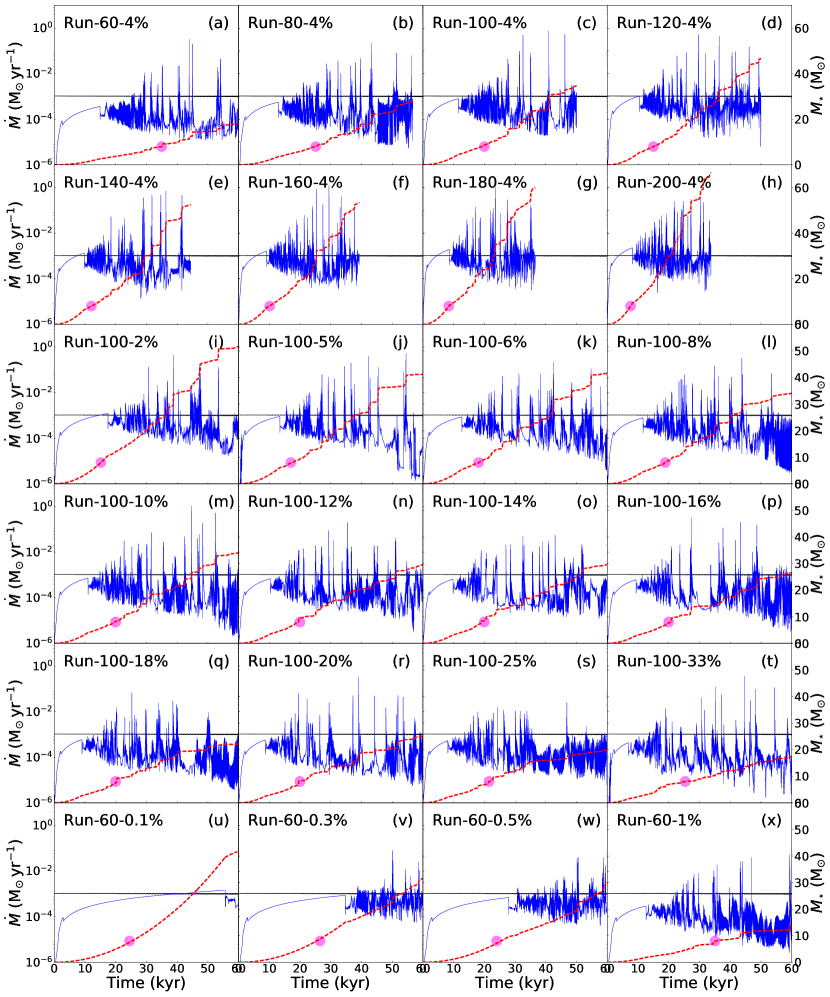
Figure 1: Accretion rate histories $\dot{M}(t)$ in our parameter study. For each 20 models, the figure shows the accretion rate (in $\rm M_{\odot}\,\rm yr^{-1}$, thin blue line) and the time evolution of the stellar mass $M_{\star}(t)$ (thick dotted red line, in $\rm M_{\odot}$). The thin horizontal black line indicates a rate of $\dot{M}=10^{-3}\,\rm M_{\odot}\,\rm yr^{-1}$, the magenta dot marks times where the protostar enters the high-mass regime ($M_{\star}=8\,\rm M_{\odot}$).

2.2 Numerical scheme, initial conditions, parameter space

The 3D models are carried out in spherical coordinates $(r,\theta,\phi)$ with a static grid. Under the simplifying assumption of the mid-plane symmetry, the size of the grid is $[r_{\rm in},r_{\rm max}]\times[0,\pi/2]\times[0,2\pi]$ along the different radial, polar and azimuthal directions. It is constructed of $128\times 21\times 128$ grid zones, while the mesh expands along $r$ as a logarithm, along $\theta$ as a cosine, and is kept uniform along $\phi$. The inner and outer boundaries are $r_{\rm in}=10\,\rm AU$ and $r_{\rm max}=R_{\rm c}=0.1\,\rm pc$, where $R_{\rm c}$ stands for the core radius, respectively. Outflow conditions are assigned at both boundaries of the radial directions $r$ so that we can measure the accretion rate onto the protostar $\dot{M}$ as the mass of the gas crossing $r_{\rm in}$. The set of above described equations are solved using a $2^{\rm nd}$ order in space and time numerical scheme with the pluto code (Mignone et al., 2007, 2012) including stellar evolution, radiation transport and self-gravity (Meyer et al., 2017, 2018). Our scheme treats the protostellar radiation, by which the photons propagate from the atmosphere of the MYSO to the accretion disc and their subsequent propagation into the disk by flux-limited diffusion performed in the gray approximation. Finally, our multidimensional scheme is solved making use of the Strang operator splitting available in the pluto code, which permits to calculate fluxes such as radiation fluxes as a series of independent one-dimensional problems.

We initialise our models with a spinning molecular core characterised by the density profile,

$$\rho(r)=K_{\rho}r^{\beta_{\rho}},$$ (19)

with $K_{\rho}$ being a constant and where $\beta_{\rho}$ is negative. The core mass that is embedded inside a given radius $r$ is,

$$M(r)=M_{\rm c}\Big{(}\frac{r}{R_{\rm c}}\Big{)}^{\beta_{\rho}+3},$$ (20)

and it determines the quantity $K_{\rho}$. Hence, one can find the density profile,

$$\rho(r)=\frac{(\beta_{\rho}+3)}{4\pi}\frac{M_{\rm c}}{R_{\rm c}^{\beta_{\rho}+3}}r^{\beta_{\rho}},$$ (21)

where $r$ is the radial coordinate. The angular momentum distribution is,

$$\Omega(R)=\Omega_{0}\Big{(}\frac{R}{r_{0}}\Big{)}^{\beta_{\Omega}},$$ (22)

with

$$R=r\sin(\theta)$$ (23)

the so-called cylindrical radius and $\Omega_{0}$ a normalization constant. It is a function of the ratio of kinetic-to-gravitational energy,

$$\beta=\frac{E_{\rm rot}}{E_{\rm grav}},$$ (24)

which fixes the initial rotation properties of the system. Finally, the cloud total gravitational energy reads

$$E_{\rm grav}=\frac{\beta_{\rho}+3}{2\beta_{\rho}+5}\frac{GM_{\rm c}^{2}}{R_{\rm c}},$$ (25)

whereas its rotational kinetic energy is,

$$E_{\rm rot}=\frac{(\beta_{\rho}+3)}{4(\beta_{\rho}+2\beta_{\Omega}+5)}\frac{\Omega_{0}^{2}M_{\rm c}r_{0}^{-2\beta_{\Omega}}}{R_{\rm c}^{-2(\beta_{\Omega}+1)}}\int_{0}^{\pi}d\theta\sin(\theta)^{3+2\beta_{\Omega}},$$ (26)

which must be solved prior to the numerical simulations to find $\Omega_{0}$. We initially set the molecular core with $\beta=4\%$. The radial profile for the distribution reads,

$$v_{\phi}(R)=R\Omega(R),$$ (27)

but $v_{\rm r}=0$ and $v_{\theta}=0$. The system’s thermal pressure is

$$p=\frac{R\rho T_{\rm c}}{\mu},$$ (28)

where $\mu$ is the mean molecular weight, $R$ is the ideal gas constant and where $T_{\rm c}=10\,\rm K$ is the core temperature. We initialise the simulations by setting,

$$T_{\rm d}=T_{\rm g}=T_{\rm c},$$ (29)

and we do not distinguish between gas and dust temperature throughout the simulation. The gas and dust temperatures are obtained by solving Eq. 17 where $E_{\mathrm{R}}$ is calculated from Eq. 10.

We run a series of simulations exploring the effects of the mass $M_{\rm c}$ and the initial ratio $\beta$ of the pre-stellar core. Instead of running the simulations up to the complete collapse of all the core material, we implicitly account for stellar feedback and its role in stopping accretion. Estimating when a protostar reaches the ZAMS is complicated, however, our stellar evolution calculations in Meyer et al. (2019) concluded that a $100\,\rm M_{\odot}$ cloud with $\beta=4\%$ produces a protostar reaching the ZAMS $\approx 50\,\rm kyr$ after the beginning of the collapse, when $M_{\rm c}/3\approx 33.3\,\rm M_{\odot}$ of the core has been accreted. This is the criterion we applied as an educated guess to terminate the simulations for the line of increasing $M_{\rm c}$. Otherwise, the mass-loading from the infalling core would continue to replenish the disk with material during the entire collapse phase if the simulation had been allowed to continue. It would thus sustain strong gravitational instability and fragmentation and hence the production of bursts which qualitative properties would remain unchanged with respect to the present study. We summarise our models in Table 1.

3 Discs properties

This section investigates the protostellar mass evolution, the mass of the accretion disc, and the ratio of the disc-to-star masses in our simulations for the formation of young massive stellar objects. We discuss these quantities for the different initial conditions of our models (masses and spins of parent pre-stellar cores).

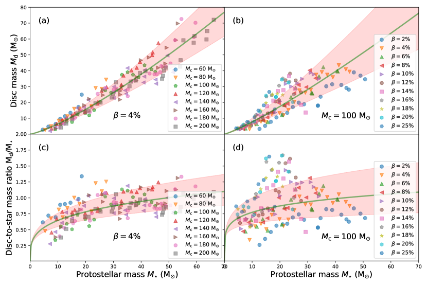
Figure 2: Disc masses $M_{\star}$ (in $\rm M_{\odot}$, top panels) and ratio of the disc-to-star masses $M_{\rm d}/M_{\star}$ (bottom panels) shown according to the protostellar mass $M_{\star}$ (in $\rm M_{\odot}$), for all models with changing core mass $M_{\rm c}$ (left panels), and for all models with changing $\beta$-ratio (right panels). The green lines show the power-law fits, respectively, and the red zone represents the errors to the fits.

3.1 Gravitational collapse and disc fragmentation

Fig. 1 reports the collection of accretion rate histories onto the MYSOs that we obtained in this parameter study. The accretion rates (thin blue line, in $\rm M_{\odot}\,\rm yr^{-1}$) are displayed starting from the early simulation time, when the gravitational collapse is initiated, up to the moment we stop the simulations, i.e. as soon as the protostellar mass has reached $M_{\star}=M_{\rm c}/3$ for the runs with changing $M_{\rm c}$ and to $60\,\rm kyr$ for the runs with changing $\beta$, respectively. The rates with different pre-stellar core mass are in Fig. 1a-h and the rates with changing $\beta$ are displayed in Fig. 1i-t. In the rest of this paper, we will refer to these series of simulations as the ”line of increasing $M_{\rm c}$” and the ”line of increasing $\beta$”, respectively, see also Vorobyov (2010, 2011b). The last series of models with $M_{\rm c}=60\,\rm M_{\odot}$ and $\beta\leq 1\%$ explores the effect of lower initial spin of the core onto the formation of high-mass stars (Fig. 1u-x).

After the very initial rise of $\dot{M}$ during the free-fall collapse of the parent molecular core, the protostar ceases accreting envelope material as the gas lands on a centrifugally-balanced disc, while it starts acquiring its mass by accretion of disc material (Fig. 1). The accretion rate shows variability once the disc has formed since it mirrors the anisotropies of the accretion flow (Meyer et al., 2018). They are caused by the development of dense spiral arms and clumps in the disc produced by efficient gravitational fragmentation. These variations in the accretion rate continue after the disc formation and they are interspersed by violent accretion spikes of increasing occurrence as the disc growths (Meyer et al., 2019). These strong bursts are repeatedly produced by the quick inward-migration of dense fragments in the disc, themselves formed by gravitational fragmentation and generating accretion-driven outbursts (Meyer et al., 2017).

The Toomre parameter estimates the disc gravitational instability by evaluating the respective effects of gas self-gravity versus that of stabilizing disc thermal pressure and rotational shear induced by Keplerian rotation (Toomre, 1963). Hence, the condition for Toomre–instability is,

$$Q=\frac{\kappa c_{\rm s}}{\pi G\Sigma}\leq Q_{\rm crit},$$ (30)

where $c_{\rm s}$ is the sound speed of the gas, $\Sigma$ the column mass density of the disc and $\kappa$ the local epicyclic frequency (Durisen et al., 2007). Fragmentation of spiral arms into compact gaseous clumps may develop if $Q_{\rm crit}\leq 1$, although recent studies derived $Q_{\rm crit}<0.6$, see the study of Meyer et al. (2018). Q-unstable discs are made of dense regions representing spiral arms, which are more prone to fragmentation (Klassen et al., 2016).

The exact nature of disc fragmentation is nevertheless a problem which complexity can not be reduced to the sole Toomre criterion. Let us review other criteria for the sake of completeness. The comparison between the local effects of disc thermodynamics regarding to the rotation-induced shear is known as the co-called Gammie-criterion that reads (Meyer et al., 2018)

$$\beta=t_{\rm cool}\Omega_{\rm K}\leq\frac{2\pi}{\sqrt{1-Q^{2}}},$$ (31)

with the Keplerian frequency,

$$\Omega_{\rm K}=\sqrt{\frac{GM_{\star}}{r^{3}}},$$ (32)

with $t_{\rm cool}$ the local cooling time-scale (Gammie, 2001). In the precedent papers of this series, we shown that this criterion, is satisfied in the warm spiral arms location as well as in the blobs, however it is not sufficient to characterise fragmentation as the interarm regions were $\beta$-unstable (Meyer et al., 2018). Note that the Gammie criterion is approximate and exclusively applies to axisymmetric accretion discs. The last criterion based on the Hill radius measures the capability of spiral arm segments to locally keep on gaining mass to eventually fragment by confronting the consequences of self-gravity versus the stellar tidal forces engendering shears in the disc (Rogers & Wadsley, 2012). A spiral arm of local cross-section $l$ is therefore subject to instability if,

$$\frac{l}{2R_{\rm Hill}}<1,$$ (33)

with $R_{\rm Hill}$ the so-called Hill radius. Material lying more than 2 $R_{\rm Hill}$ of a given region fragment will not feel the gravity of the local dense region but will have its evolution governed by the overall disc dynamics. For discs around high-mass stars, the Hill-radius-based criterion of Rogers & Wadsley (2012) has been shown to be more consistent with numerical simulations (Meyer et al., 2018).

3.2 Disc and masses of the MYSOs

Top panels of Fig. 2 show the masses $M_{\rm d}$ of the disc (in $\rm M_{\odot}$) versus the protostellar mass $M_{\star}$ (in $\rm M_{\odot}$) regarding to the line of increasing pre-stellar core mass ($\beta=4\%$, panel a) and for the line of increasing $\beta$-ratio ($M_{\rm c}=100\,\rm M_{\odot}$, panel b). For each model, the stellar mass is calculated as being a proportion of the gas mass leaving the computational domain per unit time through the inner region of the accretion disc, i.e.,

$$M_{\star}(t)=\int_{0}^{t}\dot{M}(t^{{}^{\prime}})dt^{{}^{\prime}},$$ (34)

where $t$ denotes the time at which the protostellar mass $M_{\star}=M_{\star}(t)$ is calculated. Similarly, the disc mass $M_{\rm d}(t)$ is estimated for each output of the simulation, following the method used in Klassen et al. (2016). The disc mass in the Figure is sampled starting from the end of the gravitational collapse and each data point is represented by a symbol and the color coding distinguishes the models with $M_{\rm c}=60$-$200\,\rm M_{\odot}$ (Fig. 2a) and with $\beta=2$-$25\%$ (Fig. 2b), respectively. Each coloured symbol therefore corresponds to a MYSO produced out of a distinct pre-stellar core, characterised by both a specific mass and spin. The overplotted solid green lines are fits using a power law of the model data, respectively.

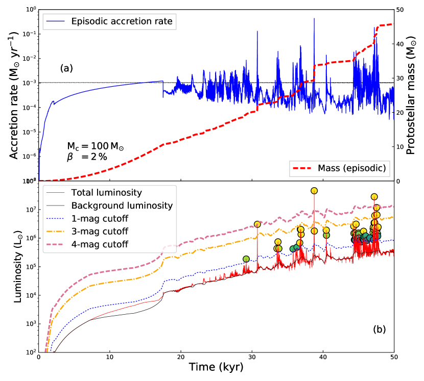
Figure 3: Top: Evolution of the accretion rate (in $\rm M_{\odot}\,\rm yr^{-1}$, thin solid line) and evolution of the mass of the protostar (in $\rm M_{\odot}$, thick dashed line) in our simulation Run-100-2$\%$. The thin horizontal black line marks a rate $\dot{M}=10^{-3}\,\rm M_{\odot}\,\rm yr^{-1}$ and the magenta dot marks when the protostar enters the high-mass regime ($M_{\star}=8\,\rm M_{\odot}$). Bottom: Total luminosity (thin solid red line, in $\rm L_{\odot}$) of the same model (b), background luminosity (thin solid black line), cut-off magnitudes for the 1-mag ($2.5$ times the background luminosity) to the 4-mag ($2.5^{4}\approx 39$ times the background luminosity) accretion bursts, respectively.

The data distribution in Fig. 2 suggests a correlation between $M_{\rm d}$ and $M_{\star}$. We perform the least-square regressions (solid green) and found the following relations,

$$\Big{(}M_{\mathrm{d,\beta=4\%}}\Big{)}=10^{-0.46\pm 0.042}\Big{(}M_{\star,\beta=4\%}^{1.27\pm 0.029}\Big{)},$$ (35)

and,

$$\Big{(}M_{\mathrm{d,\frac{M_{\rm c}}{M_{\odot}}=100}}\Big{)}=10^{-0.29\pm 0.063}\Big{(}M_{\star,\frac{M_{\rm c}}{M_{\odot}}=100}^{1.17\pm 0.049}\Big{)},$$ (36)

where the subscripts $\beta$ and $M_{\rm c}$ stand for the lines of increasing spin pre-stellar core and spin, respectively. The time sampling of the disc mass history to construct Fig. 2a may also influence the data distribution in the $M_{\rm d}$-$M_{\star}$ plane which, in its turn, make the finding of a best fit somehow uneasy. However, the power-law fits (solid green line) match fairly well except for $M_{\rm c}\gg 60\,\rm M_{\odot}$, meaning that the slope of $\approx 1.27$ is relatively good (see Eq. 35). In our example, the data for high-mass protostars are not as dispersed as those in Vorobyov (2011b) because all the considered models have the same gravitational-to-kinetic ratio $\beta=4\%$. One can immediately see that the models with the heavier pre-stellar cores $M_{\rm c}\geq 100\,\rm M_{\odot}$ are slightly off-set with respect to the fit, and that the slope of the overall fit might weaken if more models with higher pre-stellar cores $M_{\rm c}\gg 200\,\rm M_{\odot}$ will be considered.

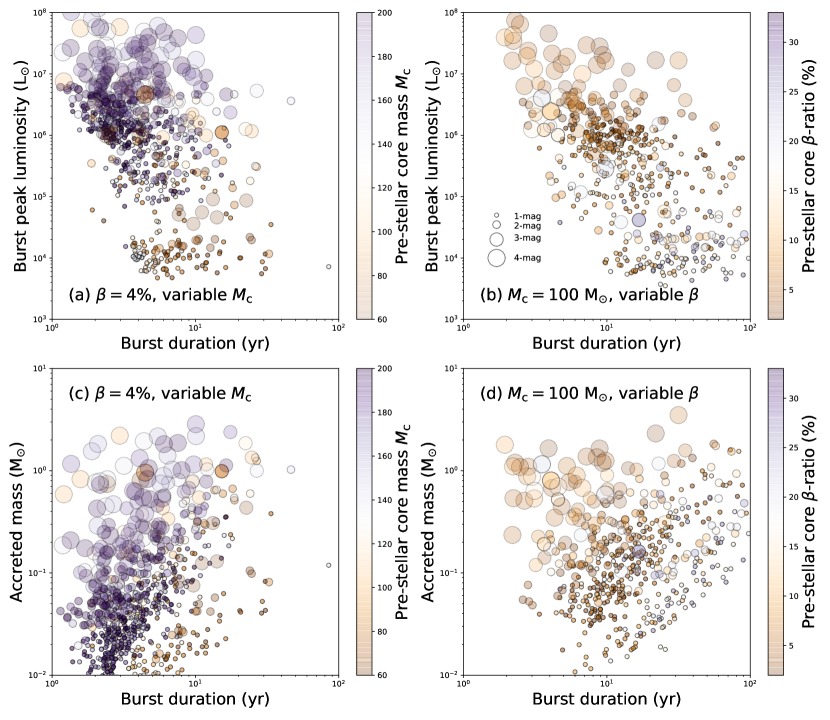
Figure 4: Scatter plots representing the burst peak luminosity versus duration of the bursts (top panels) and scatter plots displaying the accretion rate peak versus the duration of the bursts (bottom panels). Colour scales distinguish the models as a function of the pre-stellar core mass $M_{\rm c}$ (top panels) and the pre-stellar core $\beta$-ratio (bottom panels). The figures display the data for the line of increasing core mass $M_{\rm c}$ (left panels) and the line of increasing $\beta$ ratio (right panels), respectively.

In Fig. 2b we show the $M_{\rm d}$-$M_{\star}$ plane for the line of increasing $\beta$. It reveals more scattering of the data compare that for the line of increasing $M_{\rm c}$, meaning that the effect of the core spin on the mass of the disc is more important than that of the core mass. As found by Vorobyov (2011b), faster-rotating, lower-mass cores tend to form heavier discs, which results in scattering in the disc mass distribution. In our case, this happens in the $10$–$30\,\rm M_{\odot}$ range. The fit might weaken if simulation models with smaller $\beta$-ratio are added. Models with initial rotational properties such that $\beta\gg 25\%$, populating the upper part of the Figure, are rather unrealistic, despite the fact that such models for massive star formation have been produced (Klassen et al., 2016). The models that produce high scattering above the fit are also the models in which the burst activity is weakened, indicating a smaller fragmentation probability of the accretion discs in them, see Tables 3-5.

3.3 Disc-to-star mass ratio

Bottom panels of Fig. 2 show the ratio of the disc-to-star masses, defined as

$$\xi=\frac{M_{\rm d}}{M_{\ast}},$$ (37)

with $M_{\rm d}$ (in $\rm M_{\odot}$) the above discussed disc mass and $M_{\star}$ (in $\rm M_{\odot}$) the protostellar mass, respectively, for both the line of increasing pre-stellar core mass ($\beta=4\%$, panel c) and for the line of increasing $\beta$-ratio ($M_{\rm c}=100\,\rm M_{\odot}$, panel d). The disc mass evolution is sampled starting from the end of the gravitational collapse and each model is represented by a different symbol and color coding, which helps to distinguish the simulations with $M_{\rm c}=60$-$200\,\rm M_{\odot}$ (Fig. 2c) and with $\beta=2$-$25\%$ (Fig. 2d), respectively. Each coloured symbol therefore represents a single protostar which has formed out of a distinct pre-stellar core characterised with particular initial conditions of $M_{\rm c}$ and $\beta$-ratios that scan our parameter space for MYSOs. The solid green line is a fit of the model data.

The data distribution in Fig. 2 equivalently suggests a correlation between $M_{\rm d}$ and $M_{\star}$. We perform first least-square fits (solid green lines) and found that,

$$\Big{(}\xi_{\mathrm{d,\beta=4\%}}\Big{)}=10^{-0.46\pm 0.042}\Big{(}\xi_{\star,\beta=4\%}^{0.27\pm 0.029}\Big{)},$$ (38)

and,

$$\Big{(}M_{\mathrm{d,\frac{M_{\rm c}}{M_{\odot}}=100}}\Big{)}=10^{-0.29\pm 0.063}\Big{(}M_{\star,\frac{M_{\rm c}}{M_{\odot}}=100}^{0.17\pm 0.049}\Big{)},$$ (39)

where the subscripts $\beta$ and $M_{\rm c}$ stand for the lines of increasing spin pre-stellar core and spin, respectively. Fig. 2c plots the $\xi$-$M_{\star}$ correlation for the line of increasing $M_{\rm c}$. The power-law fits agree well except in the range of $M_{\star}\leq 15\,\rm M_{\star}$. The models with lower $M_{\rm c}$ populate the figure’s upper left part, above the fits, while the models with higher $M_{\rm c}$ are located in the lower part of the figure, where more statistics might exist. No model seems to have $\xi<0.25$ and all of them have $\xi>0.5$ as long as the protostellar mass has reached $M_{\star}\approx 15\,\rm M_{\odot}$. This can be explained by the substential mass gained by the discs around protostars which already entered the high-mass region, while the efficiency of mass transport via gravitational torques in their surrounding accretion discs is not strong enough to compete with the mass inflowing from the still collapsing molecular envelope. Young fragmenting discs with $\xi<0.25$ should therefore be very unusual along both the lines of increasing $M_{\rm c}$ and $\beta$ (Fig. 2d).

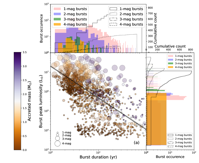
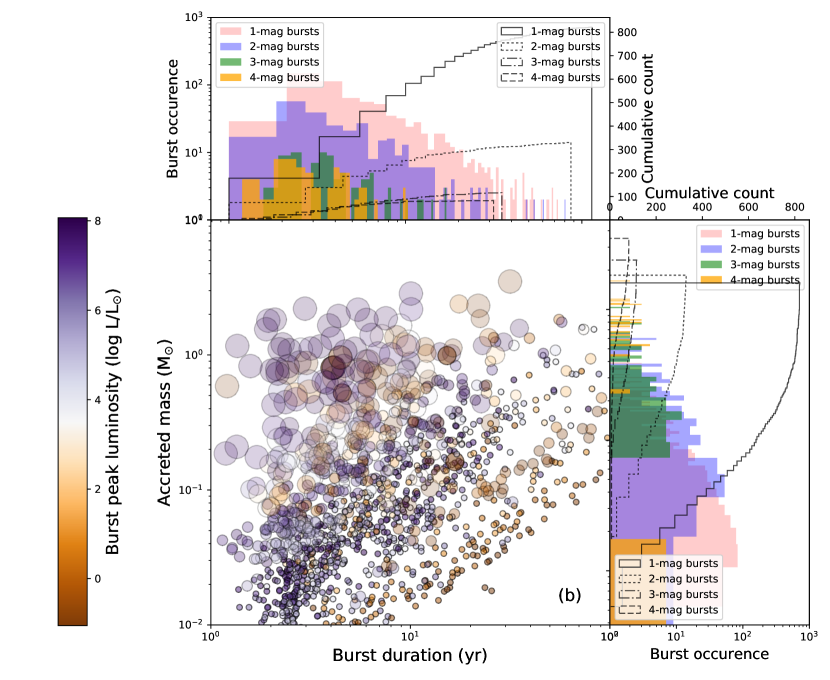
Figure 5: Scatter plots representing the burst peak luminosity as a function of the duration of the burst (top panel) and scatter plots displaying the accretion rate peak as a function of duration of the bursts (bottom panel) for all bursts in our parameter study. Colour scales distinguish the data as a function of the mass accreted by the protostar (top panel) and the bursts peak luminosity (bottom panel). The marginal histograms show the burst occurrence versus the duration of the bursts, peak luminosity and mass accreted by the protostar during each individual bursts.

The distribution of $\xi$ for the line of increasing $\beta$ is obviously more scattered than that of the line of increasing $M_{\rm c}$ as a consequence of the dispersion of the $M_{\rm c}$ distribution (see Fig. 2) and the fit of the data deviates a lot for $M_{\star}\leq 30\,\rm M_{\odot}$. Slowly-spinning pre-stellar cores will produce lighter accretion discs and therefore populate the $\xi<0.5$ region of the figure, while fast-rotating core with high $\beta$-ratio will tend to populate the upper left region of the figure in which $\xi>1.0$, respectively. The increase of $\xi$ is the direct consequence of changes in the mass transport governing mechanism in circumstellar discs. When the disc forms after the cloud collapse, $\xi$ is rather low but it quickly increases as in the disc interior no physical process can yet cope with the infalling envelope. However, when the disc gains sufficient mass for gravitational instability to occur, the resulting torques stimulate protostellar accretion and the mass begins to grow, thus decelerating the initial increase in $\xi$. As soon as inward-migration of dense and heavy clumps is triggered, accompanied by accretion bursts, the disc mass is reduced by an equivalent amount of the clump mass gained by the protostar and $\xi$ decreases, typically in the $M_{\star}\geq 30\,\rm M_{\odot}$ mass range. Again, this indicates that the variations of $\beta$-ratio in the initial conditions have a stronger effect on $\xi$ than the variations of the core mass $M_{\rm c}$.

4 Bursts properties

We perform an analysis of the accretion-driven bursts contained in the lightcurves of our MYSOs. The burst properties are investigated according to their parent core properties, and we determine how stars gain their mass, either by quiescent accretion or by accretion-driven bursts.

4.1 Protostellar luminosities

We extract from each disc simulation the protostellar lightcurves and the properties of the corresponding accretion bursts. The total luminosity of the protostars,

$$L_{\rm tot}=L_{\star}+L_{\rm acc},$$ (40)

is calculated being the luminosity $L_{\star}$ of the protostellar photosphere taken from Hosokawa & Omukai (2009), plus the accretion luminosity,

$${\color[rgb]{0,0,0}L_{\rm acc}=fG\frac{M_{\star}\dot{M}}{R_{\star}},}$$ (41)

where $M_{\star}$ is the mass of the MYSOs, $G$ is the universal gravitational constant, $\dot{M}$ denotes the protostellar mass accretion rate from the disc, and $R_{\star}$ is the protostellar radius. In Eq. (41) the coefficient $f=3/4$ stands for the proportion of mass that is considered as being accreted by the star as compared to that going in a protostellar jet/outflow (Meyer et al., 2019). Fig. 3 illustrates how the mass transport from the accretion disc to the protostellar surface affects the variations of the lightcurve.

Figure 6: Proportion of final protostellar mass gained during the quiescent phases of accretion for our models along the line of increasing core mass $M_{\rm c}$ (a, left panel) and for the line of increasing $\beta$ ratio (b, middle panel), respectively. Each orange dot represents a simulated protostar. The dashed black lines show the linear fits, respectively. The red zone represents the error interval to the fits.

We analyse the accretion bursts together with their occurrence and characteristics throughout the modelled stellar lifetime. The method separates the background secular variability, which accounts for spiral-arms-induced anisotropies formed in the disc, from the episodic accretion events caused by infalling dense gaseous clumps. We first define $L_{\rm bg}$, the so-called background luminosity, which is calculated by filtering out all accretion bursts. It reads

$$L_{\mathrm{bg}}(t)=\begin{cases}\Big{\langle}L_{\star}(t)+L_{\rm acc}(t)\Big{\rangle}&\text{if $\dot{M}\leq\dot{M}_{\rm crit}$ }\\ \Big{\langle}L_{\star}(t)+\delta L_{\rm acc}(t)\Big{\rangle}&\text{if $\dot{M}>\dot{M}_{\rm crit}$ },\end{cases}$$ (42)

where,

$$\delta=\frac{\dot{M}_{\rm crit}}{\dot{M}},$$ (43)

and with $\dot{M}_{\rm crit}=5\times 10^{-4}\,\rm M_{\odot}\,\rm yr^{-1}$, which replaces strong accretion bursts from $L_{\rm acc}$. The time averaging in Eq. (42) is $1000\,\rm yr$. We then derive the properties for the so-called $i$-mag bursts with $1\leq\mathrm{i}\leq 4$, where an $i$-mag outburst is a burst with $L_{\rm acc}\geq 2.5^{\mathrm{i}}L_{\rm bg}$ (Meyer et al., 2019). Our algorithm selecting the bursts makes sure that very mild luminosity variations smaller than 1-mag, potentially originating from boundary effects, are not qualified as physical accretion bursts and that the duration of the bursts is sufficiently short that any secular variations of $L_{\rm tot}$ are not confused with an outburst. All bursts and their properties are displayed as Appendix in our Tables 3, 4 and 5, respectively.

4.2 Bursts properties

In Fig. 4 we display the correlation between the maximum luminosity of the accretion bursts (in $\rm L_{\odot}$) versus the burst duration (in $\rm yr$) (top panels) and the bursts peak accretion rate (in $\rm M_{\odot}\,\rm yr^{-1}$) versus the burst duration (in $\rm yr$) (bottom panels), where the colour-coding representing the pre-stellar core mass $M_{\rm c}$ (in $\rm M_{\odot}$) (top panels) and its corresponding $\beta$-ratio (in $\%$) (bottom panels), respectively. The panels display the data for the line of increasing core mass $M_{\rm c}$ (left panels) and the line of increasing $\beta$ ratio (right panels), respectively. The numbers and detailed properties of those burst are reported in the Tables in the Appendix.

The meaning of this figure is described in great details in Meyer et al. (2019). Fig. 4a shows that along the line of increasing $M_{\rm c}$, the burst peak luminosity augments with $M_{\rm c}$. The burst magnitude augments as a function of the burst luminosity, except for the 4-mag bursts that are more dispersed in the figure (Table 4). Fig. 4b illustrates that the most luminous flares are typically short-duration 3-mag and 4-mag bursts. These bright outbursts are generally shorter and more luminous in models with lower $\beta$-ratio than in models with higher $\beta$. The effect of the increase of pre-stellar core $M_{\rm c}$ results in a concentration of the bursts in the small duration-high luminosity part of the diagram, except for the 1-mag bursts which do not accrete much mass (Fig. 4a). The effect of the increase of pre-stellar $\beta$-ratio results in the shift of the burst distribution to the region of longer bursts (Fig. 4b). Fig. 4c indicates that the 1-mag and 2-mag bursts accrete less mass by bursts than the 3-mag and 4-mag bursts. The most massive cores generate the shortest and least accreting bursts, while the lightest cores produce longest bursts. Fig. 4d demonstrates that models with lower $\beta$ accrete more mass and generate more 3-mag and 4-mag burst than in the simulations with higher initial core spin.

Table 2: Proportion of mass gained by the MYSOs in the quiescent phase of accretion (in $\%$). The results are shown for the line of increasing $\beta$ and $\mathrm{M}_{\rm c}$, respectively, as well as for all models together.

${\rm{Models}}$	$\mathrm{min}$ ($\%$)	$\mathrm{mean}$ ($\%$)	$\mathrm{max}$ ($\%$)
Line of increasing $\beta$	52.07	62.95	77.71
Line of increasing $\mathrm{M}_{\rm c}$	43.96	58.91	87.95
All models	43.96	61.30	87.95

In Fig. 5 we display how the burst duration (in $\rm yr$) versus the peak luminosity of the bursts (in $\rm L_{\odot}$) scatters (top panel) and the duration of the bursts (in $\rm yr$) versus their maximum accretion rate (in $\rm M_{\odot}\,\rm yr^{-1}$) (bottom panel) for each individual bursts without distinguishing the models with changing $M_{\rm c}$ and changing $\beta$. The colours indicate the mass which has been transferred from the disc to the protostar through the bursts (in $\rm M_{\odot}$) (top panel) and the peak luminosity reached during the bursts (in $\rm M_{\odot}$) (bottom panel), respectively. The bursts almost populate the entire Fig. 5a. The low-luminosity 1-mag bursts are typically in the $10^{3}$-$10^{6}\,\rm L_{\odot}$ region and they are characterized by a wide range of duration ($1$-$10^{2}\,\rm yr$). The bursts that accrete less mass are the 1-mag dimmer ones. The bursts accreting the larger amount of mass are mostly 3- and 4-mag bursts and they are distributed decreasing with the burst duration time in the upper region of the figure with respect to the fit of $L(t)$. A similar trend is visible in Fig. 5b, in which the more luminous bursts of 3- and 4-mag accrete more mass than the bursts producing dimmer 1- and 2-mag accretion-bursts. The luminous bursts are generally of shorter duration as compared to the fainter bursts which last longer. The bursts of similar magnitude and peak luminosity in Fig. 5b are distributed along diagonals (from bottom-left to upper-right), which reflects the fact that the accretion rate $\dot{M}$ varies slowly during a given burst. Therefore, if the burst duration augments, the accreted mass also increases linearly, and the bursts of similar luminosities appear as parallel diagonal lines in the mass-duration plane.

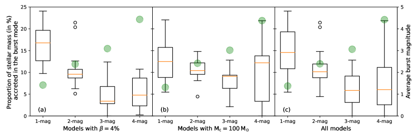
Figure 7: Box plot of the proportion of final protostellar mass accreted during the burst phases for our grid of simulated protostars. The results are displayed as a function of the burst magnitude, which can span from $2.5$ (1 magnitude bursts) to $2.5^{4}$ (4 magnitudes bursts) above the protostellar background luminosity. The orange line marks the mean value of a given series of bursts. The figures show the data for the line of increasing core mass $M_{\rm c}$ (a, left panel), the line of increasing $\beta$ ratio (b, middle panel) and for all data (c, right panel), respectively. The green dots indicate the average burst magnitude for each model.

One can note that the bursts with the largest accreted mass and shortest duration are also not necessarily the very most luminous ones (top left part of Fig. 5b). The total luminosity that we plot here reflects the variations of both the photospheric luminosity and the accretion luminosity, the latter being function of the accretion rate onto the protostar and of the inverse of the stellar radius (Meyer et al., 2019). The protostars accreting the largest amount of mass consequently see their radius bloating while going to the red part of the Hertzsprung-Russell diagram. Consequently, even tough they accrete the largest mass and generate 4-mag bursts, they are fainter than some other bursts. The energy in the bloated atmosphere is then radiated away while the protostar returns to the quiescent phase of accretion and continues its pre-ZAMS evolution towards the main-sequence. It strongly impacts the nature of the ionizing flux released in the cavity that is normal to the disc plane (see also discussion Section 5). The proper timescale of this phenomenon is difficult to predict without self-consistent stellar evolution calculations, which time-dependently account for the physics of accretion, such as the genec (Haemmerlé, 2014; Haemmerlé et al., 2016, 2017) or the stellar (Yorke & Kruegel, 1977; Hosokawa & Omukai, 2009; Hosokawa et al., 2010) codes. Only then the structure and upper layer thermodynamics of the MYSOs can be calculated. Our stellar evolution calculations previously performed with Run-100-4$\%$ showed that when experiencing a 4-mag burst, MYSOs experience a sudden rise of their luminosity that is triggered by the brutal increase of the accretion rate at the moment of a disc clump accretion (Meyer et al., 2019). This induces the formation of an upper convective layer, provoking a luminosity wave propagating outwards (Larson, 1972), and causes the swelling of the protostellar radius (Hosokawa et al., 2010).

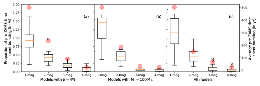
Figure 8: Box plot of the proportion of pre-zero-age-main-sequence-time (pre-ZAMS) the protostellar spend in the burst mode of accretion. The results are displayed as a function of the burst magnitude, which can span from $2.5$ (1 magnitude bursts) to $2.5^{4}$ (4 magnitudes bursts) above the protostellar background luminosity. The orange line marks the mean value of a given series of bursts. The figure shows the data for the line of increasing core mass $M_{\rm c}$ (a, left panel), the line of increasing $\beta$ ratio (b, middle panel) and for all data (c, right panel), respectively. The red dots indicate the average time the protostars spent in the burst phase (in $\rm yr$).

Our models for MYSOs show that this swelling lasts on the order of $~{}100$$-$$1000\,\rm yr$, depending on how much mass is accreted during the burst, and the protostellar flare may appear as a longer, lower amplitude burst. Furthermore, the situation is even more complex as there is no one-to-one correspondence between the accretion rate and total luminosity, as the star can act as a capacitor and release part of the accreted energy in a delayed manner. This induces a rise in the photospheric luminosity which might dominate the total luminosity in the late outburst stages when the MYSO returns to the quiescent phase. The protostellar flare may appear as a longer, lower amplitude burst. At least this can happen in the context of low-mass protostars, see Elbakyan et al. (2019). Recent observations show that some masers are very good tracers of the decrease of the radiation field, see section 3.3 of Chen et al. (2020) and Fig. 4 of Chen et al. (2020), which can be interpreted as a clue of the burst duration. The flare of NGC 6334 I is going on still and that of S255 lasted for years (Szymczak et al., 2018), and stronger flares seem to be longer.

This phenomenon is also probably influenced by the spatial resolution of the simulations, in the sense that higher resolution models will permit to better follow the collapse of the clump interiors, and by the size of the sink cell, inevitably introducing boundary effects. Indeed, our burst analysis of a higher-resolution disc model in Meyer et al. (2019) shows that the 4-mag bursts are less frequent than in those with lower resolution, although this calculation had been integrated over a more reduced time. Further simulations with a much higher spatial resolution are is necessary to address this question in more detail.

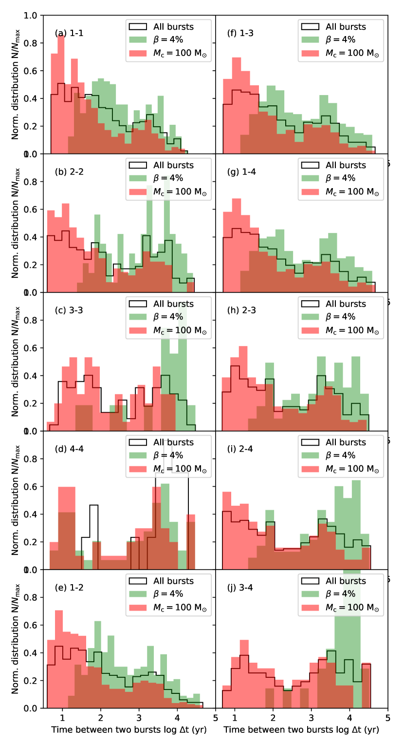
Figure 9: Normalised distribution $N/N_{\rm max}$ of the time intervals between two consecutive accretion-driven bursts in our simulations. It is calculated for each possible combination allowed by our 1-, 2-, 3- and 4-mag bursts. We present the results for the 1- to 4-mag bursts exclusively (panels a-d) while the panels e-g concerns the distribution of all consecutive bursts of magnitude 1 to 2 (1-2), 1 to 3 (1-3), and 1 to 4 (1-4), respectively. The other combinations are plotted in panels h-j. All time intervals (in $\rm yr$) are plotted in the logarithmic scale.

The marginal histograms on the right and top sides of Fig. 5a,b concern the bursts occurrence of the whole set of bursts experienced by all our protostars. The data are plotted with different colours depending on the burst magnitude, while the black lines show their cumulative occurrence. The top histograms are the same of both panels (a) and (b) as they equally represent the burst duration. Our conclusion confirms that the maximum burst duration is below $100\,\rm yr$. We confirm that bursts with shorter duration induce stronger bursts, and hence it will be more unlikely to monitor these events in the context of MYSOs, questioning the observability of 4-mag, FU-Orionis-like accretion bursts. The mass gained during a burst extends from about 10 Jupiter masses to a solar mass, which is within the limits accreted during the outburst of, e.g., S255IR-NIRS 3 (Caratti o Garatti et al., 2017). As described in Meyer et al. (2019), the distribution of accreted masses mirrors the variety of disc fragments, i.e., the clumps and dense spiral arm segments generated by gravitational instability in the disc.

We note that strongest accretion bursts may happen alongside with the formation of low-mass binary companions to MYSOs. We demonstrated in  Meyer et al. (2018) that it is possible to form simultaneously both close/spectroscopic objects around a MYSO, while it simultaneously undergoes an outburst. This happens when migrating massive clumps get rid of their envelope while contracting into a dense nucleus, thus forming a secondary low-mass protostellar core. The burst luminosity distribution indicates that 1- and 2-mag bursts are more common that 3- and 4-mag bursts. Their luminosity peak is at $\approx 10^{5}$–$10^{6}\,\rm L_{\odot}$, while the other, higher-luminosity bursts are much more uncommon. Still, there are 3-mag bursts with luminosities $\geq 10^{6}\,\rm L_{\odot}$, and a few rare 4-mag bursts peak at luminosities $\geq 10^{7}\,\rm L_{\odot}$, see also in Meyer et al. (2019).

4.3 Quiescent versus burst phases of accretion

We calculate for each simulation model the proportion of final protostellar mass that is gained either in the quiescent or during the burst phases, respectively. The minimal, mean and maximal values for the quiescent phase are reported in our Table 2 for the lines of increasing $\beta$ and $\mathrm{M}_{\rm c}$, as well as for the other simulations’ models. The models with different $\beta$-ratios indicate that the protostar acquires between $52.07\,\%$ and $77.71\,\%$ of their final mass during the quiescent phase, with a mean value of about $62.95\,\%$. The rest of the mass is therefore accreted during the time spent in the burst mode ($L_{\rm tot}\geq 2.5L_{\rm bg}$). The simulations with constant $\beta$-ratio of $4\,\%$ but changing protostellar core mass $M_{\rm c}$ have a mean value of $58.91\,\%$ with extreme value of $43.96\,\%$ and $87.95\,\%$, respectively.

Fig. 6 details the proportion of final protostellar mass gained during the quiescent phase of accretion, i.e. ignoring all burst phase, for all our models. One can see that it gradually increases with $\beta$ from $\approx 55\%$ for the model with $\beta=2\%$ to $\approx 70\%$ for the models with $\beta=33\%$ (Fig. 6a), meaning that less mass is gained in the burst mode in the case of highly-spinning cores. Inversely, the model with $M_{\rm c}=20\,\rm M_{\odot}$ spends $87.95\,\%$ of its protostellar lifetime in the quiescent phase and such quantity monotonically decreases to the model with $M_{\rm c}=200\,\rm M_{\odot}$ that spends half of its pre-main-sequence lifetime, namely $43.96\,\%$, in the quiescent mode (see Fig. 6b). It indicates that our results are more sensitive to $M_{\rm c}$ than to its initial spin. The latter governs, for a give radius and core’s structure, the duration of the free-fall gravitational collapse. Hence, the stars forming out of lightest pre-stellar cores are more prone to gain mass by quiescent disc accretion than by accretion-driven bursts, whereas the heaviest pre-stellar cores spend a larger fraction of their pre-zero-age-main-sequence in the burst phase.

In Fig. 7 we show the box plots of the fraction of the final protostellar mass accreted during the burst phase for the 1-mag ($L_{\rm tot}\geq 2.5L_{\rm bg}$) to 4-mag bursts ($L_{\rm tot}\geq 2.5^{4}L_{\rm bg}$). The figures display the data for the line of increasing core mass $M_{\rm c}$ (a, left panel), the line of increasing $\beta$ ratio (b, middle panel) and for all data (c, right panel), respectively. For each burst samples, i.e. the lines of increasing $M_{\rm c}$ (a), increasing $\beta$ (b), or both (c), we draw a box extending from the lower/first quartile $Q_{\rm L}$ (i.e. the data lower half’s median) to upper quartile $Q_{\rm U}$ (i.e. the data upper half’s median) of the considered sample, with an orange line at the median of all the data. With $\mathrm{IQR}=Q_{\rm U}-Q_{\rm L}$ being the interquartile range, the box whiskers extend from the box to $1.5\times Q_{\rm U}$ and to $1.5\times Q_{\rm L}$, respectively. Flying points marked as white circles are those past the range [$Q_{\rm L}-3\mathrm{IQR}/2$ , $Q_{\rm U}+3\mathrm{IQR}/2$]. Hence, the extend of the whiskers marks the dispersion of most bursts, except marginal ones represented as circles and laying outside of the whiskers. The green dots in the figure indicate the average magnitude of the bursts for all models. The burst magnitude is the exponent $i$ defined as,

$$\frac{L_{\rm tot}}{L_{\rm bg}}=2.5^{i},$$ (44)

which corresponds to

$$i=\frac{1}{\log(2.5)}\log\Big{(}\frac{L_{\rm tot}}{L_{\rm bg}}\Big{)},$$ (45)

with $L_{\rm tot}$ and $L_{\rm bg}$ the total luminosity and the background luminosity, respectively. The arithmetic average is then performed for both the lines of the increasing $\beta$ (Fig. 7a), and $\rm M_{\rm c}$ (Fig. 7b) and for all models (Fig. 7c). Note that the average 1-mag burst can only be in the (1-2)-mag limit, the 2-mag burst can only be in the (2-3)-mag limit, and so forth. Interestingly, the data exhibit a significant homogeneity (Fig. 7a,b) meaning that, on the average, the mean burst magnitude is independent of the pre-stellar core properties. Our approach is modelling bursts can therefore be compared to observations, see Section 5.4.

Concerning the line of increasing $M_{\rm c}$ (Fig. 7a), most mass accreted during the burst phase is gained as 1-mag bursts, with a median amount of mass $\approx 17\%$ of the final protostellar mass. The amount of material accreted during the 2- and 3-mag bursts decreases with median values of $10\%$ and $4\%$, respectively. Finally, for models at constant $\beta$-ratio, the mass accumulated during the 4-mag FU-Orionis-like bursts is slightly higher than that of the 3-mag burst, however with a larger dispersion than, e.g. the 2-mag bursts. The situation is globally similar for the line of increasing $\beta$ (Fig. 7b) as the median mass accreted by the protostar decreases from $13\%$ and $10\%$ for the 1-, 2- and 3-mag bursts, nevertheless the 4-mag bursts behave differently with a mean mass similar to that of the 1-mag bursts, but with a huge dispersion spanning from $<5\%$ to $>20\%$. This indicates that the $\beta$-ratio of the pre-stellar core affects much more the manner stars gain their mass than the initial core mass. Regarding to the whole data set (Fig. 7c), a decreasing trend of the accreted mass during the accretion phases showing bursts versus the burst magnitude is found with $14\%$, $10\%$ and $6\%$ for the 1-, 2- and 3-mag bursts, respectively, and another $6\%$ for the 4-mag burst, the latter being however attached to a huge dispersion of the values produced by differences in the models with changing $\beta$.

In Fig. 8, we display the statistics for the proportion of pre-ZAMS time the MYSOs spend in the burst mode of accretion (in $\%$), together with the average time protostars experience accretion phases that are characterised by either 1-mag, 2-mag, 3-mag or 4-mag bursts, respectively (in $\rm yr$). The models with $\beta=4\%$ have a rather large dispersion of the proportion of time they spend in 1-mag bursts, which spread between $0.25\%$ and $1.6\%$ of the calculated time, with a mean value around $\approx 1\%$. These values gradually diminish as the burst magnitude augments and we find that our MYSOs spend very little ($\leq 0.1\%$) of their time experiencing 4-mag bursts (Fig. 8a). The same is true for the models with $M_{\rm c}=100\,\rm M_{\odot}$, although the values are slightly larger for the 1-mag and the 2-mag bursts (Fig. 8b), because our models with high initial $\beta$-ratio of their molecular pre-stellar core spend more time in the burst mode than those with lower $\beta$-ratio (Table 4). The statistics for all models (Fig. 8c) therefore indicates that MYSOs spend about $2\%$ of their pre-ZAMS time in the burst mode of accretion. The rare events are the fast 4-mag bursts responsible for the excursions in the cold regions of the Hertzsprung-Russell diagram (Meyer et al., 2019). The findings in our parameter study therefore confirm the previously obtained results on the basis of a much smaller sample of massive protostars, and which stated that MYOs spend about $1.7\%$ of their early formation phase in the burst mode of accretion (Meyer et al., 2019).

5 Discussion

This section presents different caveats in our method, further discuss the results in the light of known young high-mass stars which experienced an outburst, and compare them their low-mass counterparts. Finally, we consider our outcomes by discussing them in the context of the temporal variabilities of massive protostellar jets.

5.1 Limitation of the model

Our parameter study is based on numerical models underlying assumptions regarding to the numerical methods. The simplifications have already been thoroughly discussed in our pilot paper Meyer et al. (2017). Particularly, we demonstrate therein that the discs in our simulations are adequately resolved, by comparing the Truelove criterion, i.e. the minimal inverse Jeans number, in the mid-plane of the accretion disc as a function of radius for three different grid resolutions. Note that the model Run-100-4$\%$ in our study is the Run-1 of Meyer et al. (2018), see their Figs. 11 and 12. They limitations principally concern the spatial resolution of the computational grid and the consideration of additional physical processes such as magnetic fields and associated non-ideal effects in the numerical simulations. Photoionization is neglected in our scheme because we concentrate on studying the accretion disc, not the bipolar lobes filled with ionising radiation, which develop perpendicular to it (Yorke et al., 1982; Rosen et al., 2016). That is why our computational mesh has a cosine-like grid along the polar direction, degrading the resolution of the protostellar cavity. Consequently, omitting photoionization in the scheme does not drastically change the outer disc physics ($\sim 100-1000\,\rm au$) that we concentrate on, while resulting in a substantial speed-up of the code.

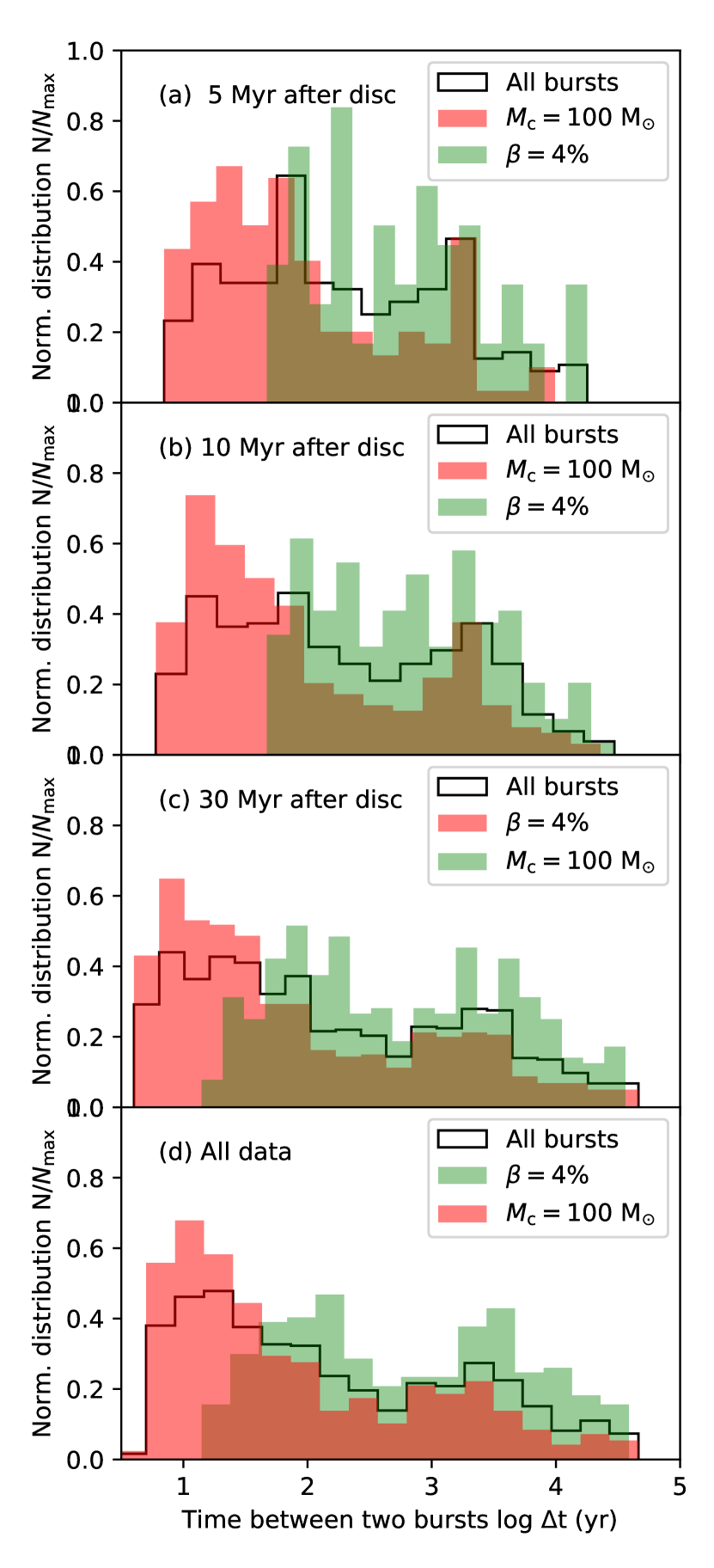
Figure 10: Time evolution of the normalised distribution $N/N_{\rm max}$ of the time intervals between two consecutive accretion-driven bursts in our simulations. It is calculated for each possible combination allowed by our 1-, 2-, 3- and 4-mag bursts. The distribution is shown at times $5\,\rm kyr$ (a), $10\,\rm kyr$ (d), and $30\,\rm kyr$ (c) once the disc has formed and for all bursts of all models (d). All time intervals (in $\rm yr$) are plotted in the logarithmic scale.

Nevertheless, this physical mechanism not only governs the ionizing flux evacuated in the outflow lobes, but also impacts the structure of accretion discs by photoevaporation (Hollenbach et al., 1994; McKee & Tan, 2008). The stellar feedback (Lyman continuum, X-ray and ultra-violet photons) irradiating the circumstellar medium can cause the ionization of the gas at the disc surface, thus leading to its evaporation as a steady flow into the ISM. Without that, the accretion flow at the disc truncation radius stops shielding the neutral disc material. It launches so-called irradiated disc winds which host complex chemical reactions between enriched species and dust particles present in the disc. This particularly happens in the late phases of disc evolution, e.g. at the T-Tauri phases or even late, when giant planets have formed and orbit inside of it, see Ercolano & Owen (2016); Weber et al. (2020); Franz et al. (2020) and references therein. One should not expect photionisation to destroy the entire discs or even to affect the development of gravitational instability in the discs (Yorke & Welz, 1996; Richling & Yorke, 1997, 1998, 2000), and consequently it should not be a determinant factor in the burst mode of accretion in massive star formation. The flux of ionizing stellar radiation is a direct function of the protostellar properties, themselves depending on the accretion history. As stated above, high accretion rates induce bloating of the stellar radius and a decrease of its effective temperature and ionizing luminosity, released either in the polar lobes or towards the equatorial plane where the disc lies. Consequently, the H ii  region generated by the protostar becomes intermittent, with variations reflecting the episodic disc accretion history onto the protostellar surface (Hosokawa et al., 2016).

With the photon flux being switch-off towards the colder part of the Herztsprung-Russell diagram during the excursions of these stars undergoing a burst, one should expect the H ii  regions to disappear when $\dot{M}$ reaches its maximum peak. The ionized lobed region then gradually reappears as the star recovers pre-ZAMS surface properties corresponding to its quiescent phase of accretion, after radiating away the clump entropy during a phase of lower-amplitude burst. Such a process has been revealed in the context of primordial, supermassive stars Hosokawa et al. (2011, 2012, 2013) We postulated that this mechanism of blinking H ii  regions should also be at work in massive star formation and constitutes a major difference between present-day young low-mass and high-mass stars (Meyer et al., 2019).

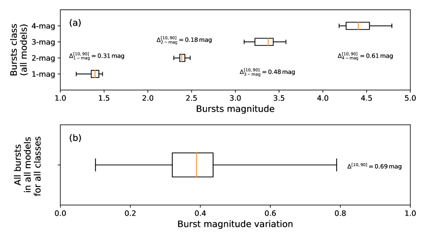
Figure 11: Box plot of the burst magnitude distribution as a function of the burst class, for all models in this study. The bursts statistics are displayed per magnitude class (a) and for all bursts of all classes in all our simulations (b). The figure indicates the magnitude difference between the $10$-th and $90$-th percentiles of each burst class.

Future improvements might principally consist of changing the initial conditions in terms of internal structures of the pre-stellar core to make it more realistic and of increasing the spatial resolution of the grid simulation, so that we can further resolve disc fragmentation when circumstellar clumps migrate in the vicinity of the protostar. Indeed, the filamentary nature of the parent pre-stellar cores in which young massive star form should definitely affect the manner star gain their mass, however, this will not support the midplane-symmetry which we impose in our simulations to divide the computational costs by a factor of $2$. Similarly, a higher spatial resolution will permit to investigate trajectories of migrating clumps to the inner disc region. Nevertheless, circumventing the caveats of our current models would be at the cost of unaffordable computational resources which will not permit a scan of the huge star formation parameter space. Longer simulations and a smaller sink cell radius $r_{\rm in}$ would also permit us to better simulate the fall, evolution, probable distortion and/or segmentation of the clumps before they are accreted onto the star. Again, this would in its turn strongly modify the time-step controlling the time-marching algorithm of the calculations and therefore the overall cost of the calculations.

5.2 Time interval between bursts

Fig. 9 displays the normalised distribution $N/N_{\rm max}$ of the time intervals between two accretion-driven bursts in our simulations,

$$\Delta=t_{j+1}^{\{i-\mathrm{mag}\}}-t_{j}^{\{i-\mathrm{mag}\}},$$ (46)

where the subscripts $j$ and $j+1$ designate two consecutive bursts selected on the basis of their magnitude ($i-\mathrm{mag}$, with $1\leq i\leq 4$) with respect to $L_{\rm bg}$. The distribution is calculated for each possible combination allowed by our 1-, 2-, 3- and 4-mag bursts. We present the results for the 1- to 4-mag bursts in Fig. 9a-d, the panels in Fig. 9e-g show the cumulative distribution of all bursts of magnitude 1 to 2 (1-2), 1 to 3 (1-3), and 1 to 4 (1-4), respectively. The other combinations are plotted in Fig. 9h-j. All time intervals are plotted in the logarithmic scale in $\rm yr$. In each panel we distinguish the results obtained for the models in the line of increasing $M_{\rm c}$ (green colour, $\beta=4\%$) and for the line of increasing $\beta=4\%$ (red colour, $M_{\rm c}=100\,\rm M_{\odot}$). The distribution including all bursts are shown with a thin black line in each panel. The number of bursts taken into account in the histograms decreases from panel (a) to panel (d) as a natural consequence of the occurrence of 1- to 4-mag bursts (Tables 3-5). Panel (g) is the plot in which all bursts in this study are considered.

Clearly, the inter-burst intervals span a wide range from several years to tens of thousands of years. When considering bursts of all durations, the short inter-burst intervals prevail. Bursts of higher amplitude (3- and 4-mag) have a bimodal distribution for the duration of quiescent phases between the bursts (Fig. 9c-d). The inclusion of 1- and 2-mag bursts diminishes the bimodality in favour of the shorter inter-burst time intervals (Fig. 9a-b). The differences between panels 9a,f and panels 9h,j highlight the fact that the bimodality is produced by the inter-burst time intervals between the lower-magnitude bursts (1,2-mag bursts) on the one hand, and the higher-magnitude bursts (3,4 mag bursts), on the other hand. The same is true for panel 9i, while the disappearance of the bimodality is obvious in panels 9e and 9f. This information may be used in future studies to compare the inter-burst time intervals with the jet spacings such as in Vorobyov et al. (2018).

Fig. 10 presents all the time intervals between the bursts calculated in our simulations during a period of $5\,\rm kyr$ (a), $10\,\rm kyr$ (b) and $30\,\rm kyr$ (c) once the disc has formed. The first three panels illustrate the development of the inter-burst time intervals as the disc evolves. The last panel (d) shows the histogram displaying the distribution of the time intervals between the bursts, for all bursts of all models and is the same distribution as in Fig. 9g. The distribution is initially rather dispersed, especially along the line of increasing $\rm M_{\rm c}$ (green bins), see Fig. 10a. At this time, the disc begins to fragment and form gaseous clumps and the bursts are still mild. The models with higher $\beta$-ratios fragment faster and therefore the corresponding inter-burst intervals are shorter (green bins) than along the line of increasing $\rm M_{\rm c}$ (red bins), see Fig. 10b-c. At later times, both series of model reach an equilibrium distribution that is made of two types of bursts separated by $\Delta t\sim\,10^{2}\,\rm yr$ and $\Delta t\geq\,10^{3}\,\rm yr$, respectively. This bimodality is further illustrated for all bursts (black line in Fig. 10d). FU-Orionis-like bursts (and therefore close binary companions) should be observed in older, massive MYSOs, surrounded by rather extended and fragmented discs.

5.3 Protostellar jets as indicators of the burst history?

Protostellar outflows and jets are part of the accretion–ejection mechanism that carries angular momentum of the accreted matter away, and thereby prevents the accreting protostar from spinning up to a break-up velocity. There are observational indications that the angles of the outflows from the high-mass young stellar object are wider for more evolved and luminous stars (Arce et al., 2007). In Meyer et al. (2019) we already mentioned that tracing of the outflows allows to show that there we about four bursts in the luminous S255 NIRS3 during a time interval of $\approx 7000\,\rm yr$ before present-day observations (Wang et al., 2011; Zinchenko et al., 2015; Burns et al., 2016) and that the burst in NGC 6334I-MM1 was not a single event (Brogan et al., 2018).

Well pronounced jets are observed in the number of the younger massive stars in the infrared and radio ranges (see, e.g. infrared survey by Caratti o Garatti et al. (2015) or radio surveys by Purser et al. (2018) and Obonyo et al. (2019). The jets manifest themselves as elongated structures in the close surroundings of the source and further knots sometimes organized in chains. So, they have potential to provide information on the history of eruptions. Protostellar jets are observed over a large source mass range (Frank et al. 2014), and recent studies show that the jets from the massive stars show similarity in physical parameters and origin with the jets from the low-mass stars (Caratti o Garatti et al., 2015; Fedriani et al., 2019).

Well-accepted is the fact that the outflowing matter may not be constant in mass and velocity. Measurements of the shock velocities in the jets from the massive stars vary from hundreds to thousands $\rm km\,\rm s^{-1}$ (McLeod et al., 2018; Purser et al., 2018). Therefore, faster material that is ejected at later times will catch up and run into slower material ahead of it, creating a new mini-bow shock. The knotty jets then are chains of these small bow-type structures. The proper motion measurements show that the dynamical times between the ejection of knots in the chains are on the order of a few decades (Eislöffel & Mundt, 1992, 1998; Devine et al., 1997), whereas the times for the larger bow-type structure at their ends are on the order of centuries, and for the largest structures in the parsec-scale jets they are even on the order of millennia (Eislöffel & Mundt, 1997; Reipurth et al., 1997). Moreover, it should be noted that the knot’s brightness in the jets from the MYSOs is subject to time variability (Obonyo et al., 2019).

The interesting question arises if these jets then are a frozen record of the accretion history of the source, and these jet knots could be used for a direct comparison with accretion events of the sources in model calculations, like the ones presented in this paper (see also Vorobyov et al. (2018)). As described above the chains of knots are not a one-to-one image of the source’s accretion history, and this principally because of possible merging of the shocks with different velocities and because the brightness of the shock knots sometimes varies with time. Little is known, however, also from a modeling point of view, whether all bursts lead to ejections of matter, how bursts can change the outflow speed, and if indeed stronger bursts are leading to faster outflowing material as well.

Keeping all the above mentioned caveats in mind, we note that in most jets with regular chains of knots the measured proper motions for each knot are not hugely different, so that one can assume that they are an indicator to a certain kind of similar burst events. At the mentioned time intervals of decades, these would then correspond to the first peak in the bi-modal burst distribution. The second peak in the bimodal burst distribution, at $10^{3}$ to $10^{4}$ years can correspond to the dynamical age of the bright knots of the jet observed in the distant source in the Large Magellanic Cloud - 8 knots are detected in the 11 pc jet with the lifetime about $28$$-$$37\,\rm kyr$ (McLeod et al., 2018). These knots probably represent the giant bow shocks seen at the end of the jets, or even multiple times in some parsec-scale jets.

5.4 What distinguishes massive star formation from its low-mass counterpart ?

5.4.1 Massive stars principally gain their mass through bursts

A series of differences between the formation processes in lower-mass and higher-mass star regimes arise from our study. First of all, our accretion histories systematically exhibit accretion variability and accretion-driven outbursts along both the lines of increasing $M_{\rm c}$ and $\beta$, but also for the models with the lowest $M_{\rm c}$ (Fig. 1). Although our results may be affected by physical mechanisms that are so far neglected, like the magnetisation of the pre-stellar core or other non-ideal magneto-hydrodynamical effects, accretion bursts seem to be a systematic feature in the formation of massive protostars. When lower-mass stellar objects form, on the contrary, accretion bursts caused by clump infall seem to exist only for cloud cores of sufficiently high mass and angular momentum (see fig. A1 in Elbakyan et al., 2019). A lower limit on the cloud core mass seems to exists also for accretion bursts triggered by the magnetorotational instability in the innermost parts of low-mass disks (Kadam et al. 2020, submitted). Our study, based on a large sample of models, confirms the conclusions of Meyer et al. (2019) stating that the MYSOs gain an important part of their final mass during the burst phase of accretion, sometimes amounting to 50% or even more. On the contrary, the low-mass stars accrete on average about 5% of their final mass with a peak value of 33% (Dunham & Vorobyov, 2012). The efficiency of gravitational instability in discs is consequently always at work in massive discs, which is consistent with the work of Kratter & Matzner (2006); Rafikov (2007, 2009), reporting that massive discs around high-mass protostars inevitably lead to fragmentation.

5.4.2 Protostars in FU-Orionis-like burst phases evolve towards the red part of the Herzsprung-Russell diagram

A series of similarities should also be underlined between the different mass regimes of star formation. Indeed, this picture of centrifugally balanced discs onto which inflowing material lands and competes with the disc thermodynamics and rotational shear equivalently applies to both regimes. Once disc fragmentation is triggered, the gaseous clumps migrate inwards, producing bursts once they are tidally destroyed near the star. Concurrently, the star migrates in the Herzsprung-Russell diagram (Elbakyan et al., 2019), irradiating the discs which should be noticed in infrared. Nevertheless, the low- and high-mass protostars show different types of excursions. The low-mass stars become bluer in the Herzsprung-Russell diagram, while the high-mass stars do it to redder, upper right part. Similar in both mass regimes is also the nearly-linear relationship between the disc and protostellar masses, the respective effects of the initial $M_{\rm c}$ and $\beta$-ratio of the pre-stellar cores onto the disc properties, implying a comparable global evolution if accretion discs at all scales and masses are ruled by analogous physical mechanisms. The observational study on young low-mass protostars by Contreras Peña et al. (2019) interestingly reports that ”Surprisingly many objects in this group show high-amplitude irregular variability over timescales shorter than $10$ years, in contrast with the view that high-amplitude objects always have long outbursts”. This is consistent with our findings in the sense that our 3- and 4-mag bursts are characterized by a wide range of burst duration (see Fig. 5). All this correspondences strongly motivate further works on the detailed features of disc fragmentation in the context of massive protostars.

5.4.3 The scatter in burst magnitudes is wider in massive star formation

We show in Fig. 11 the scattering of the burst magnitude for all bursts in our data as a function of their burst class (from the 1-mag bursts to the 4-mag ones). The box plots present the data using whiskers extending from the $10$-th to the $90$-th percentile, which allows us to visualize the extent of the variation in magnitudes for all bursts encompassed within one burst class (e.g., between 1- and 2-mag, 2- and 3-mag, etc). The variation reads

$$\Delta_{\mathrm{i-mag}}^{[10,90]}=|W_{\mathrm{i-mag}}^{\mathrm{90-th}}-W_{\mathrm{i-mag}}^{\mathrm{10-th}}|,$$ (47)

where $W_{\mathrm{i-mag}}^{\mathrm{90-th}}$ and $W_{\mathrm{i-mag}}^{\mathrm{10-th}}$ are the burst magnitude at the extent of the whiskers, respectively, and $i$ denotes a considered burst class ($1\leq i\leq 4$). The upper panel displays the bursts variation statistics for all burst in our parameter study as a function of the burst class (a) and for all the collection of bursts in our parameter study (b). We find variations of $\Delta_{\mathrm{1-mag}}^{[10,90]}=0.31\,\mathrm{mag}$, $\Delta_{\mathrm{2-mag}}^{[10,90]}=0.18\,\mathrm{mag}$, $\Delta_{\mathrm{3-mag}}^{[10,90]}=0.48\,\mathrm{mag}$ and $\Delta_{\mathrm{4-mag}}^{[10,90]}=0.61\,\mathrm{mag}$, respectively. The extend of the burst variation regardless of their magnitude class (Fig. 11b) gives $\Delta_{\mathrm{1-mag}}^{[10,90]}=0.69\,\mathrm{mag}$. Particularly, one can compare the obtained burst variations with the value of $0.22$ found for low-mass sources at $3.6\,\mu m$ in the context of low-mass stellar objects in the Serpens South star formation region (Wolk et al., 2018). According to our study, the average luminosity variation in massive star formation is larger than that in low-mass star formation, which constitutes a remarkable difference between these two regimes.

6 Conclusion

This work explores the effects of both the initial mass ($M_{\rm c}=60$–$200\,\rm M_{\odot}$) and rotational-to-gravitational energy ratio ($\beta=0.5$–$33\%$) of a representative sample of molecular pre-stellar cores by means of three-dimensional gravito-radiation-hydrodynamics simulations. We utilise the method previously detailed in Meyer et al. (2019). Our simulations model the evolution of molecular cores and how the collapsing material lands onto centrifugally balanced accretion discs surrounding young massive protostars. The efficient gravitational instability in the disc results in the aggregation of disc material in clumps within spiral structures. These blobs of gas can gravitationally fall towards the protostar and generate luminous accretion-driven outbursts (Meyer et al., 2017), affecting both the properties of the disc and its central MYSOs. We calculate in each model the accretion rate histories and lightcurves of the evolving massive protostars. As soon as a simulated protostar leaves the quiescent regime of accretion and enters the burst mode, we analyse the properties of the corresponding flare, such as its duration, peak luminosity, accreted mass, and intensity. These quantities are statistically analysed for the large sample of bursts that we extract from our grid of hydrodynamical simulations.

Under an assumption of negligible magnetic fields, which may have a major effect on accretion disc physics (Flock et al., 2011) and star formation processes (McKee et al., 2020), we found that cores with higher mass $M_{\rm c}$ and/or $\beta$-ratio tends to produce circumstellar discs more susceptible to experience accretion bursts. All massive protostars in our sample have accretion bursts, even those with pre-stellar cores of low $\beta$-ratio $\leq 1\%$. This constitutes, under our assumptions, a major difference between the mechanisms happening in the low-mass and massive regimes of star formation. All our disc masses scale as a power-law with the mass of the protostars and disc-to-mass ratios $M_{\rm d}/M_{\star}>1$ are obtained in models with higher $\beta$ or small $M_{\rm c}$, as at equal age more massive discs are obtained from cores of greater $M_{\rm c}$ but larger $\beta$. Our results confirm that massive protostars accrete about $40$-$60\%$ of their mass in the burst mode and stronger bursts appear in the later phase of the disc evolution.

Our numerical experiments keep on indicating that present-day massive formation is a scaled-up version of low-mass star formation, both being ruled by the burst mode of accretion. As for their low-mass counterparts, young massive stars experience a strong and sudden increase of their accretion rate, e.g. when a disc fragment falls onto the star. This results in large amplitude fluctuations of its total luminosity, a swelling of the stellar radius and a decrease of the flux released in the protostar’s associated H ii  region. Under our assumptions, we calculate within the $10$$-$th and $90$$-$th percentile of the collection of bursts in our simulations of forming massive stars, the extend of their luminosity variations is $\approx 0.69$, which is much larger than that observed for low-mass protostars (Wolk et al., 2018). This constitutes a major difference between the high- and low-mass regimes of star formation, to be verified by means of future observations. Last, we discuss the structure of massive protostellar jets as potential indicators of their driving star’s burst history. We propose that the high-frequency component of the burst bimodal distribution would correspond to the regular chain of knots along the overall jet morphology, while the second, low-frequency component peaking at $10^{3}$-$10^{4}\,\rm yr$ would be associated with the giant bow shock at the top of these jets. Our results motivate further investigations of the burst mode of accretion in forming higher-mass stars and its connection with the morphology of massive protostellar jets.

Data availability

This research made use of the pluto code developed at the University of Torino by A. Mignone (http://plutocode.ph.unito.it/). The figures have been produced using the Matplotlib plotting library for the Python programming language (https://matplotlib.org/). The data underlying this article will be shared on reasonable request to the corresponding author.

Table 3: Summary of burst characteristics along the line of increasing $\beta$. $N_{\mathrm{bst}}$ is the number of bursts at a given magnitude cut-off. $L_{\mathrm{max}}/L_{\mathrm{min}}/L_{\mathrm{mean}}$ are the maximum, minimum and mean burst luminosities, respectively. Similarly, $\dot{M}_{\mathrm{max}}/\dot{M}_{\mathrm{min}}/\dot{M}_{\mathrm{mean}}$ are the maximum, minimum and mean accretion rates through the central sink cell and $t_{\mathrm{bst}}^{\mathrm{max}}$/$t_{\mathrm{bst}}^{\mathrm{min}}$/$t_{\mathrm{bst}}^{\mathrm{mean}}$ are the maximum, minimum and mean bursts duration, while $t_{\mathrm{bst}}^{\mathrm{tot}}$ is the integrated bursts duration time throughout the star’s live.

Model		$N_{\mathrm{bst}}$	$L_{\mathrm{max}}/L_{\mathrm{min}}/L_{\mathrm{mean}}$ ($10^{5}\,\rm L_{\odot}$)	$\dot{M}_{\mathrm{max}}/\dot{M}_{\mathrm{min}}/\dot{M}_{\mathrm{mean}}$ ($\rm M_{\odot}\,\rm yr^{-1}$)	$t_{\mathrm{bst}}^{\mathrm{max}}$/$t_{\mathrm{bst}}^{\mathrm{min}}$/$t_{\mathrm{bst}}^{\mathrm{mean}}$ $\rm(yr)$	$t_{\mathrm{bst}}^{\mathrm{tot}}$ $\rm(yr)$
1-mag cutoff
${\rm Run-100-2}$$\%$		38	21.12 / 1.855 / 10.75	0.0194 / 0.0033 / 0.0076	81 / 5 / 16	626
${\rm Run-100-4}$$\%$		33	21.43 / 0.558 / 7.91	0.0180 / 0.0031 / 0.0068	39 / 5 / 13	444
${\rm Run-100-5}$$\%$		21	15.09 / 0.067 / 4.44	0.0190 / 0.0014 / 0.0083	88 / 9 / 26	553
${\rm Run-100-6}$$\%$		36	18.69 / 0.149 / 5.77	0.0222 / 0.0023 / 0.0094	73 / 3 / 22	807
${\rm Run-100-8}$$\%$		29	9.60 / 0.057 / 3.28	0.0301 / 0.0012 / 0.0082	53 / 5 / 15	449
${\rm Run-100-10}$$\%$		44	13.07 / 0.063 / 3.83	0.0228 / 0.0013 / 0.0060	94 / 5 / 16	705
${\rm Run-100-12}$$\%$		30	6.19 / 0.057 / 1.84	0.0198 / 0.0012 / 0.0094	110 / 4 / 26	789
${\rm Run-100-14}$$\%$		30	10.73 / 0.052 / 3.04	0.0216 / 0.0012 / 0.0081	114 / 6 / 27	806
${\rm Run-100-16}$$\%$		30	4.99 / 0.035 / 1.16	0.0209 / 0.0007 / 0.0073	76 / 7 / 28	829
${\rm Run-100-18}$$\%$		26	2.54 / 0.037 / 0.64	0.0160 / 0.0008 / 0.0054	97 / 6 / 31	794
${\rm Run-100-20}$$\%$		7	3.02 / 0.064 / 1.54	0.0241 / 0.0016 / 0.0087	78 / 5 / 27	188
${\rm Run-100-25}$$\%$		21	0.83 / 0.043 / 0.21	0.0148 / 0.0012 / 0.0048	89 / 5 / 41	855
${\rm Run-100-33}$$\%$		6	0.34 / 0.036 / 0.12	0.0116 / 0.0012 / 0.0035	79 / 12 / 39	234
Total all models		27	21.43 / 0.035 / 3.42	0.0301 / 0.0007 / 0.0072	114 / 3 / 25	622
2-mag cutoff
${\rm Run-100-2}$$\%$		13	50.44 / 17.752 / 26.67	0.0337 / 0.0127 / 0.0197	40 / 3 / 11	139
${\rm Run-100-4}$$\%$		22	45.60 / 10.495 / 26.62	0.0356 / 0.0117 / 0.0226	56 / 3 / 13	277
${\rm Run-100-5}$$\%$		6	35.66 / 6.385 / 15.34	0.0488 / 0.0104 / 0.0265	17 / 6 / 11	69
${\rm Run-100-6}$$\%$		8	35.15 / 4.124 / 23.22	0.0519 / 0.0150 / 0.0307	14 / 6 / 9	73
${\rm Run-100-8}$$\%$		11	22.62 / 0.221 / 6.81	0.0603 / 0.0044 / 0.0322	44 / 4 / 12	127
${\rm Run-100-10}$$\%$		11	27.96 / 0.201 / 8.32	0.0494 / 0.0040 / 0.0236	74 / 6 / 20	217
${\rm Run-100-12}$$\%$		8	23.31 / 0.146 / 5.18	0.0422 / 0.0031 / 0.0155	78 / 8 / 35	281
${\rm Run-100-14}$$\%$		10	12.68 / 0.144 / 3.48	0.0478 / 0.0033 / 0.0191	80 / 5 / 30	305
${\rm Run-100-16}$$\%$		7	4.25 / 0.211 / 1.10	0.0330 / 0.0042 / 0.0145	60 / 4 / 31	217
${\rm Run-100-18}$$\%$		9	3.38 / 0.188 / 1.24	0.0669 / 0.0037 / 0.0196	87 / 6 / 36	320
${\rm Run-100-20}$$\%$		7	7.63 / 0.129 / 1.75	0.0482 / 0.0035 / 0.0166	81 / 10 / 37	262
${\rm Run-100-25}$$\%$		6	2.99 / 0.150 / 0.68	0.0250 / 0.0038 / 0.0082	91 / 16 / 36	216
${\rm Run-100-33}$$\%$		10	1.84 / 0.116 / 0.46	0.0566 / 0.0031 / 0.0117	68 / 9 / 35	351
Total all models		4	50.44 / 0.116 / 9.30	0.0669 / 0.0031 / 0.0200	91 / 3 / 24	220
3-mag cutoff
${\rm Run-100-2}$$\%$		4	117.38 / 30.481 / 68.54	0.1303 / 0.0386 / 0.0711	14 / 5 / 9	37
${\rm Run-100-4}$$\%$		4	65.74 / 13.512 / 50.64	0.0537 / 0.0385 / 0.0466	29 / 4 / 13	52
${\rm Run-100-5}$$\%$		2	37.41 / 4.992 / 21.20	0.0616 / 0.0448 / 0.0532	35 / 8 / 22	43
${\rm Run-100-6}$$\%$		3	44.86 / 11.743 / 26.04	0.0663 / 0.0636 / 0.0651	16 / 6 / 11	32
${\rm Run-100-8}$$\%$		3	70.36 / 40.645 / 52.45	0.0683 / 0.0371 / 0.0558	8 / 3 / 6	18
${\rm Run-100-10}$$\%$		3	38.50 / 9.240 / 23.18	0.0708 / 0.0375 / 0.0559	8 / 3 / 6	17
${\rm Run-100-12}$$\%$		2	6.63 / 0.575 / 3.60	0.0902 / 0.0124 / 0.0513	25 / 10/ 18	35
${\rm Run-100-14}$$\%$		1	12.23 / 12.234 / 12.23	0.0525 / 0.0525 / 0.0525	4 / 4 / 4	4
${\rm Run-100-16}$$\%$		1	10.07 / 10.068 / 10.07	0.1148 / 0.1148 / 0.1148	5 / 5 / 5	5
${\rm Run-100-18}$$\%$		-	-	-	-	-
${\rm Run-100-20}$$\%$		4	15.17 / 0.384 / 7.72	0.0511 / 0.0083 / 0.0345	23 / 4 / 12	46
${\rm Run-100-25}$$\%$		1	0.42 / 0.415 / 0.42	0.0097 / 0.0097 / 0.0097	17 /17 / 17	17
${\rm Run-100-33}$$\%$		5	9.83 / 0.620 / 4.09	0.1124 / 0.0132 / 0.0738	21 / 3 / 7	35
Total all models		3	117.38 / 0.384 / 24.18	0.1303 / 0.0083 / 0.0570	35 / 3 / 11	28
4-mag cutoff
${\rm Run-100-2}$$\%$		4	456.50 / 167.523 / 277.06	0.4224 / 0.1057 / 0.2104	22 / 4 / 11	44
${\rm Run-100-4}$$\%$		5	745.03 / 140.465 / 307.95	0.5235 / 0.0929 / 0.2260	9 / 2 / 5	27
${\rm Run-100-5}$$\%$		8	644.26 / 37.481 / 221.32	0.4384 / 0.0804 / 0.2146	10 / 2 / 4	32
${\rm Run-100-6}$$\%$		2	190.73 / 166.192 / 178.46	0.2117 / 0.1108 / 0.1612	32 / 2 / 18	37
${\rm Run-100-8}$$\%$		2	195.60 / 30.315 / 112.96	0.3164 / 0.1457 / 0.2311	6 / 3 / 4	9
${\rm Run-100-10}$$\%$		4	432.37 / 100.012 / 261.88	0.9294 / 0.1007 / 0.4241	7 / 2 / 3	14
${\rm Run-100-12}$$\%$		1	24.54 / 24.540 / 24.54	0.1966 / 0.1966 / 0.1966	4 / 4 / 4	4
${\rm Run-100-14}$$\%$		-	-	-	-	-
${\rm Run-100-16}$$\%$		3	42.30 / 12.521 / 28.73	0.2903 / 0.1527 / 0.2155	5 / 3 / 4	11
${\rm Run-100-18}$$\%$		-	-	-	-	-
${\rm Run-100-20}$$\%$		2	40.11 / 2.822 / 21.47	0.3285 / 0.0600 / 0.1942	10 / 4 / 7	13
${\rm Run-100-25}$$\%$		-	-	-	-	-
${\rm Run-100-33}$$\%$		1	12.92 / 12.920 / 12.92	0.3145 / 0.3145 / 0.3145	2 / 2 / 2	2
Total all models		3	745.03 / 2.822 / 144.74	0.9294 / 0.0600 / 0.2388	32 / 2 / 6	19

Table 4: Same as Tab. 3 for the line of increasing $\rm M_{\rm c}$.

Model		$N_{\mathrm{bst}}$	$L_{\mathrm{max}}/L_{\mathrm{min}}/L_{\mathrm{mean}}$ ($10^{5}\,\rm L_{\odot}$)	$\dot{M}_{\mathrm{max}}/\dot{M}_{\mathrm{min}}/\dot{M}_{\mathrm{mean}}$ ($\rm M_{\odot}\,\rm yr^{-1}$)	$t_{\mathrm{bst}}^{\mathrm{max}}$/$t_{\mathrm{bst}}^{\mathrm{min}}$/$t_{\mathrm{bst}}^{\mathrm{mean}}$ $\rm(yr)$	$t_{\mathrm{bst}}^{\mathrm{tot}}$ $\rm(yr)$
1-mag cutoff
${\rm Run-60-4}$$\%$		30	3.28 / 0.05 / 0.74	0.022 / 0.001 / 0.008	30.8 / 2.3 / 10.5	315
${\rm Run-80-4}$$\%$		49	4.43 / 0.05 / 0.58	0.022 / 0.001 / 0.006	33.6 / 1.9 / 8.7	428
${\rm Run-120-4}$$\%$		58	17.24 / 0.06 / 4.45	0.019 / 0.001 / 0.007	18.1 / 2.6 / 5.1	296
${\rm Run-140-4}$$\%$		44	18.1 / 0.07 / 5.44	0.020 / 0.001 / 0.008	85 / 1.9 / 6.2	274
${\rm Run-160-4}$$\%$		79	22.68 / 0.79 / 10.6	0.018 / 0.003 / 0.008	17.1 / 1.6 / 3.9	309
${\rm Run-180-4}$$\%$		94	27.57 / 0.15 / 11.1	0.020 / 0.004 / 0.008	12.6 / 1.8 / 3.7	352
${\rm Run-200-4}$$\%$		103	44.07 / 0.7 / 13.56	0.022 / 0.004 / 0.010	16.2 / 1.4 / 4.0	407
Total all models		59	44.07 / 0.05 / 5.97	0.022 / 0.001 / 0.007	85 / 1.4 / 6.0	309
2-mag cutoff
${\rm Run-60-4}$$\%$		12	4.71 / 0.15 / 1.17	0.043 / 0.003 / 0.13	24.6 / 5.3 / 11.8	142
${\rm Run-80-4}$$\%$		11	5.20 / 0.12 / 1.32	0.048 / 0.003 / 0.018	32.6 / 5.3 / 13.2	145
${\rm Run-120-4}$$\%$		14	37.46 / 18.08 / 20.25	0.060 / 0.121 / 0.029	24.1 / 2.9 / 7.7	108
${\rm Run-140-4}$$\%$		16	46.55 / 2.8 / 20.28	0.058 / 0.013 / 0.03	46.4 / 1.5 / 9.8	156
${\rm Run-160-4}$$\%$		33	46.29 / 3.45 / 25.78	0.054 / 0.01 / 0.024	13.9 / 1.4 / 4.4	144
${\rm Run-180-4}$$\%$		45	75.39 / 1.84 / 28.56	0.047 / 0.013 / 0.026	12.0 / 1.4 / 4.0	182
${\rm Run-200-4}$$\%$		70	81.13 / 3.77 / 39.84	0.057 / 0.014 / 0.027	10.5 / 1.1 / 3.5	243
Total all models		53	81.13 / 0.12 / 18.17	0.060 / 0.003 / 0.067	46.4 / 1.1 / 7.6	149
3-mag cutoff
${\rm Run-60-4}$$\%$		6	0.90 / 0.36 / 0.61	0.02 / 0.008 / 0.014	22.6 / 7.7 / 13.1	78
${\rm Run-80-4}$$\%$		1	11.15	0.065	15.3	15
${\rm Run-120-4}$$\%$		8	105 / 12.65 / 51.07	0.088 / 0.051 / 0.07	22.4 / 2.0 / 6.5	52
${\rm Run-140-4}$$\%$		9	109.4 / 35.5 / 65.9	0.11 / 0.04 / 0.075	26.8 / 1.7 / 8.1	73
${\rm Run-160-4}$$\%$		9	106.4 / 36.4 / 65.7	0.119 / 0.035 / 0.059	6.5 / 1.9 / 3.6	33
${\rm Run-180-4}$$\%$		20	221.8 / 16.49 / 93.17	0.136 / 0.038 / 0.075	17.5 / 1.6 / 4.9	98
${\rm Run-200-4}$$\%$		22	217.6 / 46.35 / 92.89	0.119 / 0.036 / 0.061	16.4 / 1.7 / 4.3	96
Total all models		10	221.8 / 0.36 / 50.5	0.136 / 0.008 / 0.06	26.8 / 1.6 / 8.3	65
4-mag cutoff
${\rm Run-60-4}$$\%$		2	10.46 / 10.22 / 10.34	0.31 / 0.20 / 0.25	4.1 / 2.4 / 3.3	6.5
${\rm Run-80-4}$$\%$		1	46.16	0.215	4.5	4.5
${\rm Run-120-4}$$\%$		4	420.6 / 121.5 / 199.1	0.43 / 0.086 / 0.246	6.7 / 2.0 / 4.3	17
${\rm Run-140-4}$$\%$		7	582.2 / 224.8 / 407.1	0.446 / 0.157 / 0.318	4.4 / 1.2 / 2.5	18
${\rm Run-160-4}$$\%$		10	1171 / 55.49 / 394.3	0.87 / 0.13 / 0.33	10.1 / 1.9 / 4.9	49
${\rm Run-180-4}$$\%$		6	1025 / 89.7 / 381.6	0.86 / 0.086 / 0.307	10.1 / 1.4 / 5.6	33
${\rm Run-200-4}$$\%$		14	575 / 117.2 / 276.4	0.337 / 0.091 / 0.176	8 / 1.4 / 4.3	60
Total all models		6	1025/10.22/264.7	0.87/0.13/0.30	10.1/1.2/3.9	24

Table 5: Same as Tab. 3 for the models with $M_{\rm c}=60\,\rm M_{\odot}$ and $\beta\leq 1$.

Model		$N_{\mathrm{bst}}$	$L_{\mathrm{max}}/L_{\mathrm{min}}/L_{\mathrm{mean}}$ ($10^{5}\,\rm L_{\odot}$)	$\dot{M}_{\mathrm{max}}/\dot{M}_{\mathrm{min}}/\dot{M}_{\mathrm{mean}}$ ($\rm M_{\odot}\,\rm yr^{-1}$)	$t_{\mathrm{bst}}^{\mathrm{max}}$/$t_{\mathrm{bst}}^{\mathrm{min}}$/$t_{\mathrm{bst}}^{\mathrm{mean}}$ $\rm(yr)$	$t_{\mathrm{bst}}^{\mathrm{tot}}$ $\rm(yr)$
1-mag cutoff
${\rm Run-60-0.1}$$\%$		-	-	-	-	-
${\rm Run-60-0.5}$$\%$		4	11.88 / 5.32 / 7.83	0.0121 / 0.0063 / 0.0100	45 / 7 / 19	77
${\rm Run-60-0.8}$$\%$		10	0.70 / 0.03 / 0.15	0.0265 / 0.0011 / 0.0048	109 / 6 / 59	594
${\rm Run-60-1}$$\%$		8	15.55 / 2.11 / 8.18	0.0173 / 0.0065 / 0.0100	56 / 9 / 19	152
All models		7	15.55 / 0.03 / 5.39	0.0265 / 0.0011 / 0.0083	109 / 6 / 32	274
2-mag cutoff
${\rm Run-60-0.1}$$\%$		-	-	-	-	-
${\rm Run-60-0.5}$$\%$		2	23.41 / 11.02 / 17.21	0.0290 / 0.0255 / 0.0272	20 / 12 / 16	32
${\rm Run-60-0.8}$$\%$		10	2.32 / 0.10 / 0.56	0.0495 / 0.0027 / 0.0154	79 / 4 / 34	336
${\rm Run-60-1}$$\%$		4	25.52 / 5.80 / 14.74	0.0406 / 0.0222 / 0.0311	49 / 9 / 21	86
All models		4	25.52 / 0.10 / 10.84	0.0495 / 0.0027 / 0.0246	79 / 4 / 24	151
3-mag cutoff
${\rm Run-60-0.1}$$\%$		-	-	-	-	-
${\rm Run-60-0.5}$$\%$		-	-	-	-	-
${\rm Run-60-0.8}$$\%$		4	0.88 / 0.33 / 0.52	0.0187 / 0.0074 / 0.0111	25 / 6 / 17	70
${\rm Run-60-1}$$\%$		-	-	-	-	-
All models		4	0.88 / 0.33 / 0.52	0.0187 / 0.0074 / 0.0111	25 / 6 / 17	70

References

- Añez-López et al. (2020) Añez-López N., Osorio M., Busquet G., Girart J. M., Macías E., Carrasco-González C., Curiel S., Estalella R., Fernández-López M., Galván-Madrid R., Kwon J., Torrelles J. M., 2020, ApJ, 888, 41
- Ahmadi et al. (2018) Ahmadi A., Beuther H., Mottram J. C., Bosco F., Linz H., Henning T., Winters J. M., Kuiper R., Pudritz R., Sánchez-Monge Á., Keto E., Beltran M., Bontemps S., Cesaroni R., Csengeri T., Feng S., Galvan-Madrid R. e. a., 2018, A&A, 618, A46
- Ahmadi et al. (2019) Ahmadi A., Kuiper R., Beuther H., 2019, A&A, 632, A50
- André Oliva & Kuiper (2020) André Oliva G., Kuiper R., 2020, arXiv e-prints, p. arXiv:2008.13653
- Arce et al. (2007) Arce H. G., Shepherd D., Gueth F., Lee C. F., Bachiller R., Rosen A., Beuther H., 2007, in Reipurth B., Jewitt D., Keil K., eds, Protostars and Planets V Molecular Outflows in Low- and High-Mass Star-forming Regions. p. 245
- Beuther et al. (2019) Beuther H., Ahmadi A., Mottram J. C., Linz H., Maud L. T., Henning T., Kuiper R., Walsh A. J., Johnston K. G., Longmore S. N., 2019, A&A, 621, A122
- Boley et al. (2019) Boley P. A., Linz H., Dmitrienko N., Georgiev I. Y., Rabien S., Busoni L., Gässler W., Bonaglia M., Orban de Xivry G., 2019, arXiv e-prints, p. arXiv:1912.08510
- Bonnell et al. (1998) Bonnell I. A., Bate M. R., Zinnecker H., 1998, MNRAS, 298, 93
- Bosco et al. (2019) Bosco F., Beuther H., Ahmadi A., Mottram J. C., Kuiper R., Linz H., Maud e. a., 2019, A&A, 629, A10
- Breen et al. (2019) Breen S. L., Sobolev A. M., Kaczmarek J. F., Ellingsen S. P., McCarthy T. P., Voronkov M. A., 2019, ApJ, 876, L25
- Brogan et al. (2018) Brogan C. L., Hunter T. R., Cyganowski C. J., Chibueze J. O., Friesen R. K., Hirota T., MacLeod G. C., McGuire B. A., Sobolev A. M., 2018, ApJ, 866, 87
- Burns (2018) Burns R. A., 2018, in Tarchi A., Reid M. J., Castangia P., eds, Astrophysical Masers: Unlocking the Mysteries of the Universe Vol. 336 of IAU Symposium, Water masers in bowshocks: Addressing the radiation pressure problem of massive star formation. pp 263–266
- Burns et al. (2017) Burns R. A., Handa T., Imai H., Nagayama T., Omodaka T., Hirota T., Motogi K., van Langevelde H. J., Baan W. A., 2017, MNRAS, 467, 2367
- Burns et al. (2016) Burns R. A., Handa T., Nagayama T., Sunada K., Omodaka T., 2016, MNRAS, 460, 283
- Burns et al. (2020) Burns R. A., Sugiyama K., Hirota T., Kim K.-T., Sobolev A. M., Stecklum B., MacLeod G. C., Yonekura Y. e. a., 2020, Nature Astronomy, 4, 506
- Caratti o Garatti et al. (2017) Caratti o Garatti A., Stecklum B., Garcia Lopez R., Eisloffel J., Ray T. P., Sanna A., Cesaroni R., Walmsley C. M., Oudmaijer R. D., de Wit W. J., Moscadelli L., Greiner J., Krabbe A., Fischer C., Klein R., Ibanez J. M., 2017, Nature Physics, 13, 276
- Caratti o Garatti et al. (2015) Caratti o Garatti A., Stecklum B., Linz H., Garcia Lopez R., Sanna A., 2015, A&A, 573, A82
- Carrasco-González et al. (2010) Carrasco-González C., Rodríguez L. F., Anglada G., Martí J., Torrelles J. M., Osorio M., 2010, Science, 330, 1209
- Cesaroni et al. (2006) Cesaroni R., Galli D., Lodato G., Walmsley M., Zhang Q., 2006, Nature, 444, 703
- Cesaroni et al. (2010) Cesaroni R., Hofner P., Araya E., Kurtz S., 2010, A&A, 509, A50
- Chen et al. (2017) Chen X., Ren Z., Zhang Q., Shen Z., Qiu K., 2017, ApJ, 835, 227
- Chen et al. (2020) Chen X., Sobolev A. M., Breen S. L., Shen Z.-Q., Ellingsen S. P., MacLeod G. C. e. a., 2020, ApJ, 890, L22
- Chen et al. (2020) Chen X., Sobolev A. M., Ren Z.-Y., Parfenov S., Breen S. L., Ellingsen S. P., Shen Z.-Q., Li B., MacLeod G. C., Baan W., Brogan C., Hirota T., Hunter T. R., Linz H., Menten K., Sugiyama K., Stecklum B., Gong Y., Zheng X., 2020, Nature Astronomy
- Chini et al. (2012) Chini R., Hoffmeister V. H., Nasseri A., Stahl O., Zinnecker H., 2012, MNRAS, 424, 1925
- Contreras Peña et al. (2019) Contreras Peña C., Naylor T., Morrell S., 2019, MNRAS, 486, 4590
- Cunningham et al. (2009) Cunningham N. J., Moeckel N., Bally J., 2009, ApJ, 692, 943
- Devine et al. (1997) Devine D., Bally J., Reipurth B., Heathcote S., 1997, AJ, 114, 2095
- Dunham & Vorobyov (2012) Dunham M. M., Vorobyov E. I., 2012, ApJ, 747, 52
- Durisen et al. (2007) Durisen R. H., Boss A. P., Mayer L., Nelson A. F., Quinn T., Rice W. K. M., 2007, Protostars and Planets V, pp 607–622
- Eislöffel & Mundt (1992) Eislöffel J., Mundt R., 1992, A&A, 263, 292
- Eislöffel & Mundt (1997) Eislöffel J., Mundt R., 1997, AJ, 114, 280
- Eislöffel & Mundt (1998) Eislöffel J., Mundt R., 1998, AJ, 115, 1554
- Elbakyan et al. (2019) Elbakyan V. G., Vorobyov E. I., Rab C., Meyer D. M.-A., Güdel M., Hosokawa T., Yorke H., 2019, MNRAS, 484, 146
- Ercolano & Owen (2016) Ercolano B., Owen J. E., 2016, MNRAS, 460, 3472
- Fedriani et al. (2019) Fedriani R., Caratti o Garatti A., Purser S. J. D., Sanna A., Tan J. C., Garcia-Lopez R., Ray T. P., Coffey D., Stecklum B., Hoare M., 2019, Nature Communications, 10, 3630
- Flock et al. (2011) Flock M., Dzyurkevich N., Klahr H., Turner N. J., Henning T., 2011, ApJ, 735, 122
- Forgan et al. (2016) Forgan D. H., Ilee J. D., Cyganowski C. J., Brogan C. L., Hunter T. R., 2016, MNRAS, 463, 957
- Franz et al. (2020) Franz R., Picogna G., Ercolano B., Birnstiel T., 2020, A&A, 635, A53
- Fuente et al. (2001) Fuente A., Neri R., Martín-Pintado J., Bachiller R., Rodríguez-Franco A., Palla F., 2001, A&A, 366, 873
- Gammie (2001) Gammie C. F., 2001, ApJ, 553, 174
- Ginsburg et al. (2018) Ginsburg A., Bally J., Goddi C., Plambeck R., Wright M., 2018, ApJ, 860, 119
- Haemmerlé (2014) Haemmerlé L., 2014, PhD thesis, University of Geneva
- Haemmerlé et al. (2016) Haemmerlé L., Eggenberger P., Meynet G., Maeder A., Charbonnel C., 2016, A&A, 585, A65
- Haemmerlé et al. (2017) Haemmerlé L., Eggenberger P., Meynet G., Maeder A., Charbonnel C., Klessen R. S., 2017, A&A, 602, A17
- Harries (2015) Harries T. J., 2015, MNRAS, 448, 3156
- Harries et al. (2017) Harries T. J., Douglas T. A., Ali A., 2017, MNRAS, 471, 4111
- Hollenbach et al. (1994) Hollenbach D., Johnstone D., Lizano S., Shu F., 1994, ApJ, 428, 654
- Hosokawa et al. (2016) Hosokawa T., Hirano S., Kuiper R., Yorke H. W., Omukai K., Yoshida N., 2016, ApJ, 824, 119
- Hosokawa & Omukai (2009) Hosokawa T., Omukai K., 2009, ApJ, 691, 823
- Hosokawa et al. (2011) Hosokawa T., Omukai K., Yoshida N., Yorke H. W., 2011, Science, 334, 1250
- Hosokawa et al. (2013) Hosokawa T., Yorke H. W., Inayoshi K., Omukai K., Yoshida N., 2013, ApJ, 778, 178
- Hosokawa et al. (2010) Hosokawa T., Yorke H. W., Omukai K., 2010, ApJ, 721, 478
- Hosokawa et al. (2012) Hosokawa T., Yoshida N., Omukai K., Yorke H. W., 2012, ApJ, 760, L37
- Hunter (2019) Hunter T., 2019, in ALMA2019: Science Results and Cross-Facility Synergies Resolving the source of the massive protostellar accretion outburst in NGC6334I-MM1B. p. 91
- Ilee et al. (2018) Ilee J. D., Cyganowski C. J., Brogan C. L., Hunter T. R., Forgan D. H., Haworth T. J., Clarke C. J., Harries T. J., 2018, ApJ, 869, L24
- Ilee et al. (2016) Ilee J. D., Cyganowski C. J., Nazari P., Hunter T. R., Brogan C. L., Forgan D. H., Zhang Q., 2016, MNRAS, 462, 4386
- Jankovic et al. (2019) Jankovic M. R., Haworth T. J., Ilee J. D., Forgan D. H., Cyganowski C. J., Walsh C., Brogan C. L., Hunter T. R., Mohanty S., 2019, MNRAS, 482, 4673
- Johnston et al. (2019) Johnston K. G., Hoare M. G., Beuther H., Kuiper R., Kee N. D., Linz H., Boley P., Maud L. T., Ilee J. D., Ahmadi A., Robitaille T. P., 2019, arXiv e-prints, p. arXiv:1911.09692
- Johnston et al. (2015) Johnston K. G., Robitaille T. P., Beuther H., Linz H., Boley P., Kuiper R., Keto E., Hoare M. G., van Boekel R., 2015, ApJ, 813, L19
- Keto & Wood (2006) Keto E., Wood K., 2006, ApJ, 637, 850
- Klassen et al. (2016) Klassen M., Pudritz R. E., Kuiper R., Peters T., Banerjee R., 2016, ApJ, 823, 28
- Kobulnicky et al. (2014) Kobulnicky H. A., Kiminki D. C., Lundquist M. J., Burke J., Chapman J., Keller E., Lester K., Rolen E. K., Topel E., Bhattacharjee A., Smullen R. A., Vargas Álvarez C. A., Runnoe J. C., Dale D. A., Brotherton M. M., 2014, ApJS, 213, 34
- Kratter & Matzner (2006) Kratter K. M., Matzner C. D., 2006, MNRAS, 373, 1563
- Kraus et al. (2017) Kraus S., Kluska J., Kreplin A., Bate M., Harries T. J., Hofmann K.-H., Hone E., Monnier J. D., Weigelt G., Anugu A., de Wit W. J., Wittkowski M., 2017, ApJ, 835, L5
- Krumholz et al. (2007) Krumholz M. R., Klein R. I., McKee C. F., 2007, ApJ, 656, 959
- Laor & Draine (1993) Laor A., Draine B. T., 1993, ApJ, 402, 441
- Larson (1969) Larson R. B., 1969, MNRAS, 145, 271
- Larson (1972) Larson R. B., 1972, MNRAS, 157, 121
- Liu et al. (2020) Liu S.-Y., Su Y.-N., Zinchenko I., Wang K.-S., Meyer D. M. A., Wang Y., Hsieh I.-T., 2020, arXiv e-prints, p. arXiv:2010.09199
- MacLeod et al. (2018) MacLeod G. C., Smits D. P., Goedhart S., Hunter T. R., Brogan C. L., Chibueze J. O., van den Heever S. P., Thesner C. J., Banda P. J., Paulsen J. D., 2018, MNRAS, 478, 1077
- MacLeod et al. (2019) MacLeod G. C., Sugiyama K., Hunter T. R., Quick J., Baan W., Breen S. L., Brogan C. L., Burns R. A., Caratti o Garatti A. e. a., 2019, MNRAS, 489, 3981
- Mahy et al. (2013) Mahy L., Rauw G., De Becker M., Eenens P., Flores C. A., 2013, A&A, 550, A27
- Maud et al. (2019) Maud L. T., Cesaroni R., Kumar M. S. N., Rivilla V. M., Ginsburg A., Klaassen P. D., Harsono D. e. a., 2019, A&A, 627, L6
- Maud et al. (2018) Maud L. T., Cesaroni R., Kumar M. S. N., van der Tak F. F. S., Allen V., Hoare M. G., Klaassen P. D., Harsono D., Hogerheijde M. R. e. a., 2018, A&A, 620, A31
- Maud et al. (2017) Maud L. T., Hoare M. G., Galván-Madrid R., Zhang Q., de Wit W. J., Keto E., Johnston K. G., Pineda J. E., 2017, MNRAS, 467, L120
- McKee et al. (2020) McKee C. F., Stacy A., Li P. S., 2020, MNRAS
- McKee & Tan (2008) McKee C. F., Tan J. C., 2008, ApJ, 681, 771
- McLeod et al. (2018) McLeod A. F., Reiter M., Kuiper R., Klaassen P. D., Evans C. J., 2018, Nature, 554, 334
- Meyer et al. (2019) Meyer D. M. A., Haemmerlé L., Vorobyov E. I., 2019, MNRAS, 484, 2482
- Meyer et al. (2019) Meyer D. M. A., Kreplin A., Kraus S., Vorobyov E. I., Haemmerle L., Eislöffel J., 2019, MNRAS, 487, 4473
- Meyer et al. (2018) Meyer D. M.-A., Kuiper R., Kley W., Johnston K. G., Vorobyov E., 2018, MNRAS, 473, 3615
- Meyer et al. (2019) Meyer D. M.-A., Vorobyov E. I., Elbakyan V. G., Stecklum B., Eislöffel J., Sobolev A. M., 2019, MNRAS, 482, 5459
- Meyer et al. (2017) Meyer D. M.-A., Vorobyov E. I., Kuiper R., Kley W., 2017, MNRAS, 464, L90
- Mignone et al. (2007) Mignone A., Bodo G., Massaglia S., Matsakos T., Tesileanu O., Zanni C., Ferrari A., 2007, ApJS, 170, 228
- Mignone et al. (2012) Mignone A., Zanni C., Tzeferacos P., van Straalen B., Colella P., Bodo G., 2012, ApJS, 198, 7
- Motogi et al. (2019) Motogi K., Hirota T., Machida M. N., Yonekura Y., Honma M., Takakuwa S., Matsushita S., 2019, ApJ, 877, L25
- Obonyo et al. (2019) Obonyo W. O., Lumsden S. L., Hoare M. G., Purser S. J. D., Kurtz S. E., Johnston K. G., 2019, MNRAS, 486, 3664
- Offner & McKee (2011) Offner S. S. R., McKee C. F., 2011, ApJ, 736, 53
- Padoan et al. (2014) Padoan P., Haugbølle T., Nordlund Å., 2014, ApJ, 797, 32
- Peters et al. (2010) Peters T., Banerjee R., Klessen R. S., Mac Low M.-M., Galván-Madrid R., Keto E. R., 2010, ApJ, 711, 1017
- Purser et al. (2018) Purser S. J. D., Lumsden S. L., Hoare M. G., Cunningham N., 2018, MNRAS, 475, 2
- Purser et al. (2016) Purser S. J. D., Lumsden S. L., Hoare M. G., Urquhart J. S., Cunningham N., Purcell C. R., Brooks K. J., Garay G., Gúzman A. E., Voronkov M. A., 2016, MNRAS, 460, 1039
- Rafikov (2007) Rafikov R. R., 2007, ApJ, 662, 642
- Rafikov (2009) Rafikov R. R., 2009, ApJ, 704, 281
- Reipurth et al. (1997) Reipurth B., Bally J., Devine D., 1997, AJ, 114, 2708
- Reiter et al. (2017) Reiter M., Kiminki M. M., Smith N., Bally J., 2017, MNRAS, 470, 4671
- Richling & Yorke (1997) Richling S., Yorke H. W., 1997, A&A, 327, 317
- Richling & Yorke (1998) Richling S., Yorke H. W., 1998, A&A, 340, 508
- Richling & Yorke (2000) Richling S., Yorke H. W., 2000, ApJ, 539, 258
- Rogers & Wadsley (2012) Rogers P. D., Wadsley J., 2012, MNRAS, 423, 1896
- Rosen et al. (2016) Rosen A. L., Krumholz M. R., McKee C. F., Klein R. I., 2016, MNRAS, 463, 2553
- Rosen et al. (2019) Rosen A. L., Li P. S., Zhang Q., Burkhart B., 2019, ApJ, 887, 108
- Samal et al. (2018) Samal M. R., Chen W. P., Takami M., Jose J., Froebrich D., 2018, MNRAS, 477, 4577
- Sanna et al. (2019) Sanna A., Kölligan A., Moscadelli L., Kuiper R., Cesaroni R., Pillai T., Menten K. M., Zhang Q., Caratti o Garatti A., Goddi C., Leurini S., Carrasco-González C., 2019, A&A, 623, A77
- Sanna et al. (2017) Sanna A., Moscadelli L., Surcis G., van Langevelde H. J., Torstensson K. J. E., Sobolev A. M., 2017, A&A, 603, A94
- Seifried et al. (2011) Seifried D., Banerjee R., Klessen R. S., Duffin D., Pudritz R. E., 2011, MNRAS, 417, 1054
- Shchekinov & Sobolev (2004) Shchekinov Y. A., Sobolev A. M., 2004, A&A, 418, 1045
- Shu (1977) Shu F. H., 1977, ApJ, 214, 488
- Szymczak et al. (2018) Szymczak M., Olech M., Wolak P., Gérard E., Bartkiewicz A., 2018, A&A, 617, A80
- Testi (2003) Testi L., 2003, in De Buizer J. M., van der Bliek N. S., eds, Galactic Star Formation Across the Stellar Mass Spectrum Vol. 287 of Astronomical Society of the Pacific Conference Series, Intermediate Mass Stars (Invited Review). pp 163–173
- Toomre (1963) Toomre A., 1963, ApJ, 138, 385
- Vorobyov (2009) Vorobyov E. I., 2009, ApJ, 704, 715
- Vorobyov (2010) Vorobyov E. I., 2010, ApJ, 723, 1294
- Vorobyov (2011a) Vorobyov E. I., 2011a, ApJ, 728, L45
- Vorobyov (2011b) Vorobyov E. I., 2011b, ApJ, 729, 146
- Vorobyov & Basu (2006) Vorobyov E. I., Basu S., 2006, ApJ, 650, 956
- Vorobyov & Basu (2010) Vorobyov E. I., Basu S., 2010, ApJ, 719, 1896
- Vorobyov & Basu (2015) Vorobyov E. I., Basu S., 2015, ApJ, 805, 115
- Vorobyov et al. (2018) Vorobyov E. I., Elbakyan V. G., Plunkett A. L., Dunham M. M., Audard M., Guedel M., Dionatos O., 2018, A&A, 613, A18
- Wang et al. (2011) Wang Y., Beuther H., Bik A., Vasyunina T., Jiang Z., Puga E., Linz H., Rodón J. A., Henning T., Tamura M., 2011, A&A, 527, A32
- Weber et al. (2020) Weber M. L., Ercolano B., Picogna G., Hartmann L., Rodenkirch P. J., 2020, MNRAS, 496, 223
- Wolk et al. (2018) Wolk S. J., Günther H. M., Poppenhaeger K., Winston E., Rebull L. M., Stauffer J. R., Gutermuth R. A., Cody A. M., Hillenbrand L. A., Plavchan P., Covey K. R., Song I., 2018, AJ, 155, 99
- Wurster & Bate (2019a) Wurster J., Bate M. R., 2019a, MNRAS, 486, 2587
- Wurster & Bate (2019b) Wurster J., Bate M. R., 2019b, arXiv e-prints, p. arXiv:1906.12276
- Yorke et al. (1982) Yorke H. W., Bodenheimer P., Tenorio-Tagle G., 1982, A&A, 108, 25
- Yorke & Kruegel (1977) Yorke H. W., Kruegel E., 1977, A&A, 54, 183
- Yorke & Sonnhalter (2002) Yorke H. W., Sonnhalter C., 2002, ApJ, 569, 846
- Yorke & Welz (1996) Yorke H. W., Welz A., 1996, A&A, 315, 555
- Zhao et al. (2018) Zhao B., Caselli P., Li Z.-Y., Krasnopolsky R., 2018, MNRAS, 473, 4868
- Zinchenko et al. (2015) Zinchenko I., Liu S.-Y., Su Y.-N., Salii S. V., Sobolev A. M., Zemlyanukha P., Beuther H., Ojha D. K., Samal M. R., Wang Y., 2015, ApJ, 810, 10
- Zinchenko et al. (2019) Zinchenko I. I., Liu S.-Y., Su Y.-N., Wang K.-S., Wang Y., 2019, arXiv e-prints, p. arXiv:1911.11447