Model-based Reinforcement Learning from Signal Temporal Logic Specifications

Abstract

Techniques based on Reinforcement Learning (RL) are increasingly being used to design control policies for robotic systems. RL fundamentally relies on state-based reward functions to encode desired behavior of the robot and bad reward functions are prone to exploitation by the learning agent, leading to behavior that is undesirable in the best case and critically dangerous in the worst. On the other hand, designing good reward functions for complex tasks is a challenging problem. In this paper, we propose expressing desired high-level robot behavior using a formal specification language known as Signal Temporal Logic (STL) as an alternative to reward/cost functions. We use STL specifications in conjunction with model-based learning to design model predictive controllers that try to optimize the satisfaction of the STL specification over a finite time horizon. The proposed algorithm is empirically evaluated on simulations of robotic system such as a pick-and-place robotic arm, and adaptive cruise control for autonomous vehicles.

I Introduction

Reinforcement learning (RL) [1] is a general class of algorithms that enable automated controller synthesis, where a high-level task/objective is coupled with repeated trial-and-error simulations to learn a policy that satisfies the given specification. Relatively recent developments in deep learning have renewed interest in designing scalable RL algorithms for highly complex systems [2, 3, 4, 5]. While many recent works have focused on so-called model-free learning, these algorithms are typically computationally expensive and model-free policies are slow to train, as they are not sample efficient. A promising approach to increase sample efficiency is model-based reinforcement learning (MBRL) [6, 7, 8]. The goal here is to (approximately) learn a predictive model of the system and use this learned model to synthesize a controller using sampling-based methods like model predictive control (MPC) [9, 10]. Another advantage of MBRL is that as the learned dynamics models are task-independent they can be used to synthesize controllers for various tasks in the same environment.

An important problem to address when designing and training reinforcement learning agents is the design of reward functions [1]. Reward functions are a means to incorporate knowledge of the goal in the training of an RL agent, using hand-crafted and fine-tuned functions of the current state of the system. Poorly designed reward functions can lead to the RL algorithm learning a policy that fails to accomplish the goal, cf. [11]. Moreover, in safety-critical systems, the agent can learn a policy that performs unsafe or unrealistic actions, even though it maximizes the expected total reward [11]. The problem of an RL agent learning to maximize the total reward by exploiting the reward function, and thus performing unwanted or unsafe behavior is called reward hacking [12].

With learning-enabled components being used increasingly commonly in real-world applications like autonomous cars, there has been an increased interest in the provably safe synthesis of controllers, especially in the context of RL [13, 14]. Work in safe RL has explored techniques from control theory and formal methods to design provably safe controllers [13, 15, 16]; and to specify tasks by synthesizing reward functions from formal specifications [14, 17, 18].

Reward hacking has been addressed by using Temporal Logics like Linear Temporal Logic (LTL) and Signal Temporal Logic (STL) to specify tasks and create reward functions, as these logics can be used to specify complex tasks in a rich and expressive manner. The authors in [14, 18] explore the idea of using the robust satisfaction semantics of STL to define reward functions for an RL procedure. Similar ideas were extended by to a related logic for RL-based control design for Markov Decision Processes (MDP) in [19].

Although these techniques are effective in theory, in practice, they do not typically scale well to the complexity of the task and introduce large sampling variance in learned policy. This is especially true in the case of tasks that have a large planning horizons, or have sequential objectives. In contrast, using Temporal Logic-based motion planning has been used successfully together with model predictive control [20, 21], where a predefined model is used to predict and evaluate future trajectories.

In this paper, we are interested in incorporating model-based reinforcement learning with Signal Temporal Logic-based trajectory evaluation. The main contributions of this paper are as follows:

1. We formulate a procedure to learn a deterministic predictive model of the system dynamics using deep neural networks. Given a state and a sequence of actions, such a predictive model produces a predicted trajectory over a user-specified time horizon.

2. We use a cost function based on the quantitative semantics of STL to evaluate the optimality of the predicted trajectory, and use a black-box optimizer that uses evolutionary strategies to identify the optimal sequence of actions (in an MPC setting).

3. We demonstrate the efficacy of our approach on a number of examples from the robotics and autonomous driving domains.

II Preliminaries

II-A Model-based Reinforcement Learning

In more traditional forms of controller design, like model predictive control [9], a major step in the design process is to have a model of the system dynamics or some approximation of it, which is in-turn used as constraints in a receding horizon optimal control problem. In MBRL, this step is automated through a learning-based algorithm that approximates the system dynamics by assuming that the system can be represented by a Markov Decision Process, and the transition dynamics can be learned by fitting a function over a dataset of transitions.

A Markov Decision Process (MDP) is a tuple $M=\left(S,A,T,\rho\right)$ where $S$ is the state space of the system; $A$ is the set of actions that can be performed on the system; and $T:S\times A\times S\to[0,1]$ is the transition (or dynamics) function, where $T(\bm{s},\bm{a},\bm{s}^{\prime})=\operatorname{\mathrm{Pr\,}}\left\lparen\bm{s}^{\prime}\nonscript\>\middle|\allowbreak\nonscript\>\mathopen{}\bm{s},\bm{a}\right\rparen$; and $\rho$ is a user-supplied evaluation metric defined on either a transition of the system (like a reward function) or over a series of transitions.

The goal of reinforcement learning (RL) is to learn a policy that maximizes $\rho$ on the given MDP. In model-based reinforcement learning (MBRL), a model of the dynamics is used to make predictions on the trajectory of the system, which is then used for action selection. The forward dynamics of the model $T$ is typically learned by fitting a function $\hat{F}$ on a dataset $\mathcal{D}$ of sample transitions $(\bm{s},\bm{a},\bm{s}^{\prime})$ collected from simulations or real-world demonstrations. We will use $\hat{F}_{\theta}(\bm{s}_{t},\bm{a}_{t})$ to denote the learned discrete-time dynamics function, parameterized by $\theta$, that takes the current state $\bm{s}_{t}$ and an action $\bm{a}_{t}$, and outputs a distribution over the set of possible successor states $\bm{s}_{t+\delta t}$.

II-B Model Predictive Control

Model Predictive Control (MPC) [9] refers to a class of online optimization algorithms used for designing robust controllers for complex dynamical systems. MPC algorithms typically involve creating a model of the system (physics-based or data-driven), which is then used to predict the trajectory of a system over some finite horizon. The online optimizer in an MPC algorithm computes a sequence of actions that optimizes the predicted trajectories given a trajectory-based cost function (such as $\rho$) . This optimization is typically done in a receding horizon fashion, i.e., at each step during the run of the controller, the horizon is displaced towards the future by executing only the first control action and re-planning at every next step. Formally, the goal in MPC is to optimize $\rho$ over the space of all fixed length action sequences. For example, let an action sequence be denoted $\bm{A}_{t}^{(H)}=(\bm{a}_{t},\ldots,\bm{a}_{t+H-1})$, then at every time step $t$ during the execution of the controller for a finite planning horizon $H$ we solve the following optimization problem:

$$\begin{split}\operatorname*{maximize}_{\bm{A}_{t}^{(H)}}\quad&\rho(\bm{\hat{s}}_{t},\bm{a}_{t},\bm{\hat{s}}_{t+1},\ldots,\bm{a}_{t+H-1},\bm{\hat{s}}_{t+H})\\ \text{ where }\quad&\bm{\hat{}}{s}_{t}=\bm{s}_{t}\\ &\bm{\hat{}}{s}_{t+i+1}=\hat{F}(\bm{\hat{s}}_{t+i},\bm{a}_{t+i}),\quad\text{ for }i\in 0,\ldots,H-1\end{split}$$ (1)

where, $\hat{F}$ is the (approximate) system dynamics model.

Notice that the system dynamics are directly encoded as constraints in the optimization problem: if the model is a linear system model, one can use Mixed Integer Linear Programming, or Quadratic Programming to solve the optimization problem at each step [22, 23]. For nonlinear systems, this problem gets significantly harder, and can be solved using nonlinear optimization techniques [24], sampling based optimizers like Monte-Carlo methods [25], the Cross-Entropy Method [26], or evolutionary strategies, like CMA-ES [27] and Natural Evolutionary Strategies [28].

II-C Signal Temporal Logic

Signal Temporal Logic (STL) [29] is a real-time logic, typically interpreted over signals over a dense-time domain that take values in a continuous metric space (such as $\mathbb{R}^{m}$). The basic primitive in STL is a signal predicate $\mu$ – a formula of the form $f(\bm{s}_{t})\geq c$, where $f$ is a function from the value domain $\mathbb{R}_{\geq 0}$ to $\mathbb{R}$, and $c\in\mathbb{R}$. STL formulas are then defined recursively using Boolean combinations of sub-formulas, or by applying an interval-restricted temporal operators to a sub-formula. In this paper, we consider a restricted fragment of STL (where all temporal operators are unbounded). The syntax of our fragment of STL is formally defined as follows:

$$\varphi::=\mu\mid\neg\varphi\mid\varphi\wedge\varphi\mid\mathbf{G}\varphi\mid\mathbf{F}\varphi\mid\varphi\mathbf{U}\varphi$$ (2)

Here, $I=[a,b]$ denotes an arbitrary time-interval, where $a,b\in\mathbb{R}_{\geq 0}$. The Boolean satisfaction semantics of STL are defined recursively over the structure of an STL formula; in lieu of the Boolean semantics, we instead present the quantitative semantics of STL and explain how these relate to the Boolean semantics. The quantitative semantics of an STL formula $\varphi$ are defined in terms of a robustness value $\rho(\varphi,\xi,t)$ that maps the suffix of the signal $\xi$ starting from time $t$ to a real value. This value (approximately) measures a signed distance by which the signal can be perturbed before its (Boolean) satisfaction value changes. A positive value implies that the signal is satisfied, while a negative robustness value implies that the systems violates the specification. Formally, the approximate robustness value (or simply robustness) is defined using the following recursive semantics [29]:

$$\begin{array}[]{r@{\hspace{.2em}}c@{\hspace{.4em}}l}\rho(f(\xi)\geq c,\xi,t)\hskip 1.99997pt&\equiv\hfil\hskip 3.99994pt&f(\xi_{t})-c\\ \rho(\neg\varphi,\xi,t)\hskip 1.99997pt&\equiv\hfil\hskip 3.99994pt&-\rho(\varphi,\xi,t)\\ \rho(\varphi_{1}\wedge\varphi_{2},\xi,t)\hskip 1.99997pt&\equiv\hfil\hskip 3.99994pt&\min(\rho(\varphi_{1},\xi,t),\rho(\varphi_{2},\xi,t))\\ \rho(\mathbf{G}\varphi,\xi,t)\hskip 1.99997pt&\equiv\hfil\hskip 3.99994pt&\inf_{t^{\prime}\geq t}\rho(\varphi,\xi,t^{\prime})\\ \rho(\mathbf{F}\varphi,\xi,t)\hskip 1.99997pt&\equiv\hfil\hskip 3.99994pt&\sup_{t^{\prime}\geq t}\rho(\varphi,\xi,t^{\prime})\\ \rho(\varphi_{1}\mathbf{U}\varphi_{2},\xi,t)\hskip 1.99997pt&\equiv\hfil\hskip 3.99994pt&\displaystyle\sup_{t^{\prime}\geq t}\!\!\min\!\left(\!\!\begin{array}[]{l}\rho(\varphi_{2},\xi,t^{\prime}),\\ \displaystyle\inf_{t^{\prime\prime}\in[t,t^{\prime})}\rho(\xi,\varphi_{1},t^{\prime\prime})\end{array}\!\!\right)\!\!\end{array}$$ (3)

The convention is that $\xi\models\varphi$ if $\rho(\varphi,\xi,0)\geq 0$, and $\xi$ does not satisfy $\varphi$ otherwise.

III Robust Controller Synthesis with Approximate Model

We now present a framework that combines the use of model-based reinforcement learning (MBRL) and sampling-based model predictive control (MPC) to maximize the robustness value of a trajectory against a given STL formula. We first learn a deterministic neural network model of the system, $\hat{F}$, which can be used to predict what the next state will be, given the current state and an action. We then use this model in an MPC setting described in Equation 1, where we use the model to sample trajectories over a finite horizon, $H$, and use CMA-ES to optimize a sequence of actions, $\bm{A}_{t}^{(H)}$, that maximizes the robustness of the predicted trajectory against an STL specification, $\varphi$.

III-A Learning the System Dynamics

Algorithm 1 Learning the system dynamics model.

1:Initialize empty dataset, $\mathcal{D}$

2:for $i\in 1,\ldots,N_{\text{traj}}$ do

3:     for Each time step $t$ do

4:         $\bm{a}_{t}\sim\textsf{Uniform}(\cdot),\bm{s}_{t+1}\sim\textsf{Env}(\bm{s}_{t},\bm{a}_{t})$

5:         $\mathcal{D}\leftarrow(\bm{s}_{t},\bm{a}_{t},\bm{s}_{t+1})$

6:     end for

7:end for

8:$\theta\leftarrow\textsf{SGD}(\mathcal{D})$

In MBRL, an approximate model of the system dynamics is learned through repeated sampling of the environment. This model can be represented using various means, including by the use of Gaussian Processes [8, 30] and, more recently, Deep Neural Networks [31, 32, 33]. Here, we represent the learned dynamics, $\hat{F}_{\theta}(\bm{s}_{t},\bm{a}_{t})$ as a deep neural network, where $\theta$ is the vector of parameters of the NN. The learned dynamics, $\hat{F}_{\theta}$, is deterministic, i.e., it outputs a single prediction on the what the change in the state of the system, $\Delta\bm{\hat{s}}_{t}=\bm{s}_{t+1}-\bm{s}_{t}$ will be, rather than outputting a distribution on the predicted states. The same design decisions were taken in [31], where they use MBRL as a preceding step to accelerate the convergence of a model-free reinforcement learning algorithm. The steps to train the model can be seen in Algorithm 1.

Collecting data

To generate the dataset, $\mathcal{D}$, of samples $\left(\bm{s},\bm{a},\bm{s}^{\prime}\right)$, we assume that we have access to some simulator, for example, the OpenAI Gym [34]. We sample a large number of trajectories (and hence, a large number of transitions), where each trajectory start at some initial state initial state $\bm{s}_{0}$ from the environment, and actions are sampled from a random controller, i.e., we pick actions from a uniform distribution over the action space of the environment.

Preprocessing the dataset

After generating the data, we calculate the target as $\Delta\bm{\hat{s}}=\left(\bm{s^{\prime}}-\bm{s}\right)$. We then calculate the mean and standard deviation for the inputs $\left(\bm{s},\bm{a}\right)$ and target outputs. We rescale the data by subtracting the mean from it and dividing it by standard deviation. This normalization aids the model training process and leads to accurate predictions for all dimensions in the state space.

Training the model

We train $\hat{F}_{\theta}(\bm{s},\bm{a})$ by minimizing the sum of squared error loss for each transition, $(\bm{s},\bm{a},\bm{s}^{\prime})$, in the dataset as follows:

$$\mathcal{L}(\theta)=\sum_{(\bm{s},\bm{a},\bm{s^{\prime}})\in\mathcal{D}_{\text{train}}}{\left(\bm{s}^{\prime}-\hat{F}_{\theta}(\bm{s},\bm{a})\right)}^{2},$$ (4)

where $\mathcal{D}_{\text{train}}$ is a partition on the dataset $\mathcal{D}$ allocated for training data. We use the remaining partition, $\mathcal{D}_{\text{val}}$, of the dataset as a validation dataset, over which we calculate the same loss described in Equation 4. The loss minimization is carried out using stochastic gradient descent, where the dataset is split into randomly sampled batches and the loss is minimized over these batches.

III-B Sampling-based Model Predictive Control

Algorithm 2 Model Predictive Control using $\hat{F}_{\theta}$.

1:for Each time step $t$ in episode do

2:     for  $1\ldots N_{\text{iter}}$ and $1\ldots N_{\text{samples}}$  do

3:         $\bm{A}_{t}^{(H)}=(\bm{a}_{t},\ldots,\bm{a}_{t+H-1})\sim\text{CMA-ES}()$

4:         for $i\in 0,\ldots,H-1$ do

5:              $\bm{\hat{s}}_{t+i+1}=\hat{F}_{\theta}(\bm{\hat{s}}_{t+i},\bm{\hat{a}}_{t+i})$

6:         end for

7:         Compute cost $\rho(\bm{\hat{s}}_{t},\bm{a}_{t},\bm{\hat{s}}_{t+1},\ldots,\bm{a}_{t+H-1},\bm{\hat{s}}_{t+H})$

8:         Update $\text{CMA-ES}()$

9:     end for

10:     Execute first action $\bm{a}^{*}$ from optimal sequence $\bm{A}_{t}^{(H)}\sim\text{CMA-ES}()$

11:end for

Once we have an approximate dynamics model, $\hat{F}_{\theta}$, where the parameters $\theta$ have been trained as in the previous section, we can use this model in a model predictive control setting.

At state $\bm{s}_{t}$, our goal is to compute a sequence of actions, $\bm{A}_{t}^{(H)}=(\bm{a}_{t},\ldots,\bm{a}_{t+H-1})$, for some finite horizon, $H$. As stated earlier, this can be formulated as an optimization problem over sampled trajectories, as described in Equation 1, and the optimization is performed using the CMA-ES [27] black-box optimizer. During each iteration of the optimizer, a number of action sequences are sampled from the optimizer’s internal distribution, and a trajectory is computed for each action sequence by repeatedly applying $\hat{F}(\bm{\hat{s}}_{t+i},\bm{a}_{t+i})$ to get $\bm{\hat{s}}_{t+i+1}$ (here, $\bm{\hat{s}}_{t}=\bm{s}_{t}$). These trajectories are then used as an input to compute the robust satisfaction value, or robustness, of the sequence of actions, given a STL specification $\varphi$, which is used as the objective function to maximize by CMA-ES. At each step, we execute only the first action given to us by CMA-ES, and perform the optimization loop at each step. The pseudocode for this can be seen in Algorithm 2.

IV Experimental Results and Discussions

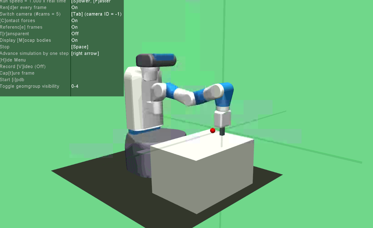
(a) Fetch Robot

(b) Highway Cruise Control

Figure 1: Examples of environments used for evaluation.

(a) Cartpole

(b) Mountain Car

(c) Highway

(d) Parking Lot

(e) Fetch robot

Figure 2: Model learning losses for each environment. The plot measures the average decay of loss with the number of training iterations across 7 different training runs.

We evaluate our framework, we train dynamics models for multiple different environments, and evaluate the model performance in the model predictive control setting. In this section, we will describe the environments we used, the tasks defined on them, and the results of using the proposed deep model predictive control framework on them, which can be seen in Table I.

Remark. It should be noted that to train the models, we chose a random controller to create the transition dataset as, in the environments we are studying, we saw that a random controller strategy for exploration of the state and action spaces works either just as good as, or sometimes better than, other methods that trade off between exploration for new transitions and exploitation of previous knowledge.

IV-A Cartpole

This is the environment described in [35], where a pole is attached to a cart on an unactuated joint. The cart moves on a frictionless track, and is controlled by applying a force to push it left or right on the track. The state vector for the environment is $\left(\theta,x,\dot{\theta},\dot{x}\right)$, where $\theta$ is the angular displacement of the pole from vertical; $x$ is the displacement of the cart from the center of the track; and $\dot{\theta}$ and $\dot{x}$ are their corresponding velocities.

The requirement, as described in [35], is to balance the pole for as long as possible on the cart (maintain angular displacement between $\pm 12^{\circ}$). For our experiments, we try to maximize the robustness of the following specification:

$$\varphi:=\mathbf{G}\left(\lvert x\rvert<0.1\land\lvert\theta\rvert<12^{\circ}\right)$$ (5)

The above specification requires that, at all time steps, the cart displacement shouldn’t exceed a magnitude of $0.1$ and the angular displacement of the pole should not exceed a magnitude of $12^{\circ}$.

In Table I, we see that for a horizon length of $10$, we are able to maximize the robustness — which is upper bounded by $0.1$ as, when the positional and angular displacement are $0$, the robustness will be the minimum distance from violation, which is $0.1$. The minor loss of robustness can be attributed to the stochasticity in the environment dynamics, making it impossible to perfectly balance the pole from time $0$. Moreover, across multiple evaluation runs, the controller is also able to maximize the rewards obtained from the environment under the standard rewarding scheme, which is $+1$ for each time step that the pole is balanced on the cart, for a maximum of 200 time steps. Specifically, the controller is able to attain a total reward of 200 consistently, across multiple runs.

IV-B Mountain Car

This environment describes a mountain climbing task, as described in [36]. The environment consists of a car stuck at the bottom of a valley between two mountains, and the car can be controlled by applying a force pushing it left or right. The state vector for the cart is on a one-dimensional left-right track, $x,\dot{x}$, where $x$ is the displacement of the cart on the track, and $\dot{x}$ is the car’s velocity along the horizontal track.

The goal of this environment is to synthesize a controller that pushes the car to the top of the mountain on the right. Under a traditional rewarding scheme, the controller is rewarded a large positive amount for reaching the top of the mountain, and a small negative amount for every step it doesn’t reach the top. We encode this specification using the following STL formula, which requires that the cart should eventually reach the top of the right side hill:

$$\varphi:=\mathbf{F}\left(x>0.4\right),$$ (6)

where $0.4$ is the horizontal coordinate of the top of the mountain on the right side.

Here, since the goal is to reach a configuration, the maximum robustness is positive only when it actually reaches the goal. Thus, any positive robustness implies a successful controller, as seen in Table I. The classical rewarding scheme is as follows, for every time step that the car hasn’t reached the goal, it gets a reward of $-0.1*action^{2}$, and only gets a positive $100$ reward when it actually reaches the top of the hill. A solution algorithm is considered to ”solve” the problem if it achieves a reward of 90.0 averaged over multiple evaluations. One key take away from this is that our controller is able to achieve this reward despite not having this requirement encoded in specifications explicitly!

IV-C Fetch robot

We use the OpenAI Gym FetchReach environment [37], where the goal of the environment is design a controller to move the arm of a simulated Fetch manipulator robot [38] to a region in 3D space. The state vector of the environment is a 16 dimensional vector containing the position and orientation of the robots joints and end-effector. The below specification is defined solely on the position of the end-effector, denoted $\left(x,y,z\right)$, and the position of the goal $\left(x_{g},y_{g},z_{g}\right)$:

$$\varphi:=\mathbf{F}\left(\lvert x_{g}-x\rvert<0.1\land\lvert y_{g}-y\rvert<0.1\land\lvert z_{g}-z\rvert<0.1\right)$$ (7)

Similar to the previous reach specification, we see that the controller learned for the FetchReach environment is able to attain a positive reward on average and a 100 percent success rate, thus satisfying the specification.

IV-D Adaptive Cruise-Control

Here, we simulate an adaptive cruise-control (ACC) scenario on a highway simulator [39]. Here, the goal is to synthesize a controller for a car (referred to as the ego car) that safely does cruise control in the presence of an adversarial (or ado) car ahead of it. The environment itself is a single lane, and the ego car is controlled only by the throttle/acceleration applied to the car. The ado agent ahead of the car accelerates and decelerates in an erratic manner, in an attempt to cause a crash.

The state space of the environment is $\left(x_{\text{ego}},v_{\text{ego}},a_{\text{ego}},d_{\text{rel}},v_{\text{rel}}\right)$, where $x_{\text{ego}}$, $v_{\text{ego}}$, and $a_{\text{ego}}$ are the position, velocity, and acceleration of the ego car on the highway; and $d_{\text{rel}}$ and $v_{\text{rel}}$ are, respectively, the relative displacement and velocity of the ado car relative to the ego car’s coordinate frame. We have the following requirements for the cruise controller:

$$\varphi:=\mathbf{F}\mathbf{G}(50>d_{\text{rel}}>15)$$ (8)

To aid the model learning process, augment the above state space with the relative acceleration of the ado car, $a_{\text{rel}}$. This is done by maintaining a difference between $v_{\text{rel}}$ between two consecutive time steps. Augmenting the state space with this manual (and trivial) estimation allows for more stable and consistent predictions by the model.

The above specification is a stable goal specification, that is, the formula requires that the ego car comes so some stable configuration eventually in the future. Thus, for any final configuration that maintains the relative distance between the ego and ado cars at a value between $15$ and $50$ satisfies the specification. In Table I, we see that the robustness $\rho$ is consistently positive and, since the robustness is the distance to violation, we see that it is well within the bounds (by $\sim 7$ units).

IV-E Parking Lot

We use the same simulator [39] used in the previous environment to simulate a parking lot, where we design a controller to park a car in a specific spot. Here, the state of the system is described on the 2D coordinate space of the parking lot surface,

$$\left(x,y,v_{x},v_{y},\cos(\theta),\sin(\theta),x_{g},y_{g}\right),$$

where $x,y$ are the position; $v_{x},v_{y}$ are the velocity components; $\theta$ is the bearing angle of the car; and $x_{g},y_{g}$ are the coordinates of the parking spot.

We evaluate the controller using the following specifications:

$$\varphi:=\mathbf{F}\left(\lvert x_{g}-x\rvert<0.02\land\lvert y_{g}-y\rvert<0.02\right)$$ (9)

Similar to Mountain Car and FetchReach, we see that this specification is also a reach requirement. Thus, any positive value close to $0$ is considered a success. This is exactly what we see in Table I.

IV-F Discussion and Analysis

TABLE I: Hyperparameters and Results.

Environment	Hyperparameters				Results (averaged across 30 runs)
	No. of training trajectories	No. of optimizer iterations	No. of optim. samples per iteration	Horizon	Trajectory Robustness	Vanilla rewards
	$N_{\text{traj}}$	$N_{\text{iter}}$	$N_{\text{samples}}$	$H$	$\rho$
Cartpole	2000	5	1000	10	$0.069\pm{8}\mathrm{e}{-3}$	$200.0\pm 0$
Mountain Car	2000	2	1000	50	$0.047\pm{1}\mathrm{e}{-3}$	$89.06\pm 4.57$
Fetch	2000	7	500	10	$0.067\pm{6}\mathrm{e}{-3}$	–
ACC	400	7	500	2	$7.679\pm 5.47$	–
Parking Lot	400	5	5	5	${1.69}\mathrm{e}{-2}\pm{3.8}\mathrm{e}{-3}$	–

In the experimental results in Table I, we see that using a deterministic model suffices for predicting trajectories as we are able to maximize the robustness and, if applicable, the rewards for a given system and specification. This even applies to complex environments like Adaptive Cruise-Control, where we have an adversarial car performing erratic behavior. We speculate that this is due to the noise in the system being time-invariant, thus predicting the mean configuration of the system is sufficiently accurate for the controller.

V Related Work

Model-based Reinforcement Learning

Model-free deep reinforcement learning algorithms based on Q-learning [2, 40], actor-critic methods [3, 4, 41], and policy gradients [42, 5] have been used to directly learn policies for specific tasks in highly complex systems including simulated robotic locomotion, driving, video game playing, and navigation. While these methods have been successful and popular, they tend to require an incredibly large number of samples and extensive computational capabilities. In contrast, in MBRL, the goal is to learn a model of the system through repeatedly acting on the environment and observing state transition dynamics, and then use this model to synthesize a controller [6] or use an under-approximation to aid in exploration of the state space [43].

Gaussian Processes [44] have been used extensively as non-parametric Bayesian models in various MBRL problems where data-efficiency is critical [7, 45, 8, 30]. In recent years, neural network-based models have generally supplanted GPs in MBRL [46, 47, 31, 48, 32, 33], as neural networks have fixed-time runtime execution, and can generalize better to complex, non-linear, high-dimensional systems. Moreover, they perform much better than Gaussian Processes in the presence of large amount of data, as in the case of RL.

Recent work has used sampling-based model predictive control (MPC) along with deep neural network dynamics models, where an optimizer outputs a sequence of actions which are used to predict trajectories, and, in-turn, the cost of the sequence of actions. The work by [31] uses a deterministic NN model with a random search optimizer for computing an action sequence. On the other hand, the work in [32] uses an ensemble of probabilistic models to output a probability distribution over the future states, and uses the Cross-Entropy Method for optimizing the sequence of actions that maximize predicted trajectory rewards.

Formal Methods in Controller Synthesis

Temporal logics have been used extensively in the context of cyber-physical systems to encode temporal dependencies in the state of a system in an expressive manner [49, 50, 51]. Originating in program synthesis and model checking literature, temporal logics like Linear Temporal Logic, Metric Temporal Logic, and Signal Temporal Logic, have been used extensively to synthesize controllers for complex tasks, including motion planning [52, 53] and synthesizing controllers for various robot systems, including swarms [54, 21, 55]. Such synthesis algorithms typically have strong theoretical guarantees on the correctness, safety, or stability of the controlled system.

A lot of traditional control theoretical approach to synthesis with STL specifications have relied on optimizing the quantitative semantics, or robustness, of trajectories generated by the controller. In [53, 55], STL specifications are used to synthesize control barrier certificates for motion planning, and in [21], the authors develop an extension to STL to reason explicitly about stochastic systems, named “Probabilistic STL” (PrSTL). Quantitative semantics for STL have been directly encoded into model predictive control optimization problems to design controllers for robots [56, 57].

Safe Reinforcement Learning

Temporal logics have been proposed as a means to address various problem in reinforcement learning. One such problem is reward hacking. This refers to cases where a reinforcement learning agent learns a policy that performs unsafe or unrealistic actions, though it maximizes the expected total reward [11, 12]. A means to approach this problem is reward shaping [58]. The work in [14] proposes an extension to Q-learning [59] where STL robustness is directly used to define reward functions over trajectories in an MDP. The approach presented in [18] translate STL specifications into locally shaped reward functions using a notion of “bounded horizon nominal robustness”, while the authors in [19] propose a method that augments an MDP with finite trajectories, and defines reward functions for a truncated form of Linear Temporal Logic.

Likewise, temporal logics have been used with model-based learning to prove the safety of a controller that has been designed for the learned models. An example of this is [13], where the authors propose a PAC learning algorithm that has been constrained using Linear Temporal Logic specifications. This is done by learning the transition dynamics of the product automaton between the unknown model and the omega-regular automaton corresponding to the LTL specification, while simultaneously using value-iteration to improve on the policy. The work by [15] uses Gaussian process models to learn the system dynamics, while using approximations of Lyapunov functions to design a controller using the learned models. Using a similar model learning approach, the authors in [60] propose the use of learning a specialized dynamics model that takes into account safe exploration using barrier certificates, while generating control barrier certificate-based policies.

VI Conclusion

In this paper, we propose a model-based reinforcement learning technique that uses simulations of the robotic system to learn a dynamical predictive model for the system dynamics, represented as a deep neural network (DNN). This model is used in a model-predictive control setting to provide finite-horizon trajectories of the system behavior for a given sequence of control actions. We use formal specifications of the system behavior expressed as Signal Temporal Logic (STL) formula, and utilize the quantitative semantics of STL to evaluate these finite trajectories. At each time-step an online optimizer picks the sequence of actions that yields the lowest cost (best reward) w.r.t. the given STL formula, and uses the first action in the sequence as the control action. In other words, the DNN model that we learn is used in a receding horizon model predictive control scheme with an STL specification defining the trajectory cost. The actual optimization over the action space is performed using evolutionary strategies. We demonstrate our approach on several case studies from the robotics and autonomous driving domain.

References

- [1] R. S. Sutton and A. G. Barto, Reinforcement Learning: An Introduction, 2nd ed., ser. Adaptive Computation and Machine Learning Series. Cambridge, Massachusetts: The MIT Press, 2018.
- [2] V. Mnih, K. Kavukcuoglu, D. Silver, A. A. Rusu, J. Veness, M. G. Bellemare, A. Graves, M. Riedmiller, A. K. Fidjeland, G. Ostrovski, S. Petersen, C. Beattie, A. Sadik, I. Antonoglou, H. King, D. Kumaran, D. Wierstra, S. Legg, and D. Hassabis, “Human-level control through deep reinforcement learning,” Nature, vol. 518, no. 7540, pp. 529–533, Feb. 2015.
- [3] T. P. Lillicrap, J. J. Hunt, A. Pritzel, N. Heess, T. Erez, Y. Tassa, D. Silver, and D. Wierstra, “Continuous control with deep reinforcement learning,” arXiv:1509.02971 [cs, stat], July 2019. [Online]. Available: http://arxiv.org/abs/1509.02971
- [4] J. Schulman, P. Moritz, S. Levine, M. Jordan, and P. Abbeel, “High-Dimensional Continuous Control Using Generalized Advantage Estimation,” arXiv:1506.02438 [cs], Oct. 2018. [Online]. Available: http://arxiv.org/abs/1506.02438
- [5] J. Schulman, F. Wolski, P. Dhariwal, A. Radford, and O. Klimov, “Proximal Policy Optimization Algorithms,” arXiv:1707.06347 [cs], Aug. 2017. [Online]. Available: http://arxiv.org/abs/1707.06347
- [6] C. Atkeson and J. Santamaria, “A comparison of direct and model-based reinforcement learning,” in Proceedings of International Conference on Robotics and Automation, vol. 4, Apr. 1997, pp. 3557–3564 vol.4.
- [7] J. Kocijan, R. Murray-Smith, C. Rasmussen, and A. Girard, “Gaussian process model based predictive control,” in Proceedings of the 2004 American Control Conference, vol. 3, June 2004, pp. 2214–2219 vol.3.
- [8] M. P. Deisenroth and C. E. Rasmussen, “PILCO: A Model-Based and Data-Efficient Approach to Policy Search,” in In Proceedings of the International Conference on Machine Learning, 2011.
- [9] E. F. Camacho and C. B. Alba, Model Predictive Control. Springer Science & Business Media, Jan. 2013.
- [10] D. Q. Mayne, J. B. Rawlings, C. V. Rao, and P. O. M. Scokaert, “Constrained model predictive control: Stability and optimality,” Automatica, vol. 36, no. 6, pp. 789–814, June 2000.
- [11] J. Leike, M. Martic, V. Krakovna, P. A. Ortega, T. Everitt, A. Lefrancq, L. Orseau, and S. Legg, “AI Safety Gridworlds,” arXiv:1711.09883 [cs], Nov. 2017. [Online]. Available: http://arxiv.org/abs/1711.09883
- [12] D. Amodei, C. Olah, J. Steinhardt, P. Christiano, J. Schulman, and D. Mané, “Concrete Problems in AI Safety,” arXiv:1606.06565 [cs], July 2016. [Online]. Available: http://arxiv.org/abs/1606.06565
- [13] J. Fu and U. Topcu, “Probably Approximately Correct MDP Learning and Control With Temporal Logic Constraints,” in Robotics: Science and Systems X, vol. 10, July 2014. [Online]. Available: http://www.roboticsproceedings.org/rss10/p39.html
- [14] D. Aksaray, A. Jones, Z. Kong, M. Schwager, and C. Belta, “Q-Learning for robust satisfaction of signal temporal logic specifications,” in 2016 IEEE 55th Conference on Decision and Control (CDC), Dec. 2016, pp. 6565–6570.
- [15] F. Berkenkamp, M. Turchetta, A. Schoellig, and A. Krause, “Safe Model-based Reinforcement Learning with Stability Guarantees,” in Advances in Neural Information Processing Systems 30, I. Guyon, U. V. Luxburg, S. Bengio, H. Wallach, R. Fergus, S. Vishwanathan, and R. Garnett, Eds. Curran Associates, Inc., 2017, pp. 908–918. [Online]. Available: http://papers.nips.cc/paper/6692-safe-model-based-reinforcement-learning-with-stability-guarantees.pdf
- [16] L. Wang, E. A. Theodorou, and M. Egerstedt, “Safe Learning of Quadrotor Dynamics Using Barrier Certificates,” arXiv:1710.05472 [cs], Oct. 2017. [Online]. Available: http://arxiv.org/abs/1710.05472
- [17] M. Hasanbeig, A. Abate, and D. Kroening, “Logically-Constrained Reinforcement Learning,” arXiv:1801.08099 [cs], Jan. 2018. [Online]. Available: http://arxiv.org/abs/1801.08099
- [18] A. Balakrishnan and J. V. Deshmukh, “Structured Reward Shaping using Signal Temporal Logic specifications,” in 2019 IEEE/RSJ International Conference on Intelligent Robots and Systems (IROS), Nov. 2019, pp. 3481–3486.
- [19] X. Li, C.-I. Vasile, and C. Belta, “Reinforcement learning with temporal logic rewards,” in 2017 IEEE/RSJ International Conference on Intelligent Robots and Systems (IROS), Sept. 2017, pp. 3834–3839.
- [20] S. S. Farahani, V. Raman, and R. M. Murray, “Robust Model Predictive Control for Signal Temporal Logic Synthesis,” IFAC-PapersOnLine, vol. 48, no. 27, pp. 323–328, Jan. 2015.
- [21] D. Sadigh and A. Kapoor, “Safe Control under Uncertainty with Probabilistic Signal Temporal Logic,” in Robotics: Science and Systems XII, vol. 12, June 2016. [Online]. Available: http://www.roboticsproceedings.org/rss12/p17.html
- [22] M. V. Kothare, V. Balakrishnan, and M. Morari, “Robust constrained model predictive control using linear matrix inequalities,” Automatica, vol. 32, no. 10, pp. 1361–1379, Oct. 1996.
- [23] A. Richards and J. How, “Mixed-integer programming for control,” in Proceedings of the 2005, American Control Conference, 2005., June 2005, pp. 2676–2683 vol. 4.
- [24] F. Allgöwer and A. Zheng, Nonlinear model predictive control. Birkhäuser, 2012, vol. 26.
- [25] A. Mesbah, “Stochastic Model Predictive Control: An Overview and Perspectives for Future Research,” IEEE Control Systems Magazine, vol. 36, no. 6, pp. 30–44, Dec. 2016.
- [26] Z. I. Botev, D. P. Kroese, R. Y. Rubinstein, and P. L’Ecuyer, “The Cross-Entropy Method for Optimization,” in Handbook of Statistics, ser. Handbook of Statistics, C. R. Rao and V. Govindaraju, Eds. Elsevier, Jan. 2013, vol. 31, pp. 35–59.
- [27] N. Hansen, The CMA Evolution Strategy: A Comparing Review, 2006.
- [28] D. Wierstra, T. Schaul, T. Glasmachers, Y. Sun, J. Peters, and J. Schmidhuber, “Natural evolution strategies,” The Journal of Machine Learning Research, vol. 15, no. 1, pp. 949–980, Jan. 2014.
- [29] A. Donzé and O. Maler, “Robust Satisfaction of Temporal Logic over Real-Valued Signals,” in Formal Modeling and Analysis of Timed Systems, ser. Lecture Notes in Computer Science, K. Chatterjee and T. A. Henzinger, Eds. Berlin, Heidelberg: Springer, 2010, pp. 92–106.
- [30] M. P. Deisenroth, D. Fox, and C. E. Rasmussen, “Gaussian Processes for Data-Efficient Learning in Robotics and Control,” IEEE Transactions on Pattern Analysis and Machine Intelligence, vol. 37, no. 2, pp. 408–423, Feb. 2015.
- [31] A. Nagabandi, G. Kahn, R. S. Fearing, and S. Levine, “Neural Network Dynamics for Model-Based Deep Reinforcement Learning with Model-Free Fine-Tuning,” arXiv:1708.02596 [cs], Dec. 2017. [Online]. Available: http://arxiv.org/abs/1708.02596
- [32] K. Chua, R. Calandra, R. McAllister, and S. Levine, “Deep Reinforcement Learning in a Handful of Trials using Probabilistic Dynamics Models,” in Advances in Neural Information Processing Systems 31, S. Bengio, H. Wallach, H. Larochelle, K. Grauman, N. Cesa-Bianchi, and R. Garnett, Eds. Curran Associates, Inc., 2018, pp. 4754–4765.
- [33] A. Nagabandi, K. Konoglie, S. Levine, and V. Kumar, “Deep Dynamics Models for Learning Dexterous Manipulation,” arXiv:1909.11652 [cs], Sept. 2019. [Online]. Available: http://arxiv.org/abs/1909.11652
- [34] G. Brockman, V. Cheung, L. Pettersson, J. Schneider, J. Schulman, J. Tang, and W. Zaremba, “OpenAI Gym,” arXiv:1606.01540 [cs], June 2016. [Online]. Available: http://arxiv.org/abs/1606.01540
- [35] A. G. Barto, R. S. Sutton, and C. W. Anderson, “Neuronlike adaptive elements that can solve difficult learning control problems,” IEEE Transactions on Systems, Man, and Cybernetics, vol. SMC-13, no. 5, pp. 834–846, Sept. 1983.
- [36] A. W. Moore, “Efficient Memory-based Learning for Robot Control,” Tech. Rep., 1990.
- [37] M. Plappert, M. Andrychowicz, A. Ray, B. McGrew, B. Baker, G. Powell, J. Schneider, J. Tobin, M. Chociej, P. Welinder, V. Kumar, and W. Zaremba, “Multi-Goal Reinforcement Learning: Challenging Robotics Environments and Request for Research,” arXiv:1802.09464 [cs], Mar. 2018. [Online]. Available: http://arxiv.org/abs/1802.09464
- [38] M. Wise, M. Ferguson, D. King, E. Diehr, and D. Dymesich, “Fetch and freight: Standard platforms for service robot applications,” in Workshop on Autonomous Mobile Service Robots, 2016.
- [39] E. Leurent, “An environment for autonomous driving decision-making,” GitHub repository, 2018. [Online]. Available: https://github.com/eleurent/highway-env
- [40] S. Gu, T. Lillicrap, I. Sutskever, and S. Levine, “Continuous deep Q-learning with model-based acceleration,” in Proceedings of the 33rd International Conference on International Conference on Machine Learning - Volume 48, ser. ICML’16. New York, NY, USA: JMLR.org, June 2016, pp. 2829–2838.
- [41] V. Mnih, A. P. Badia, M. Mirza, A. Graves, T. Lillicrap, T. Harley, D. Silver, and K. Kavukcuoglu, “Asynchronous Methods for Deep Reinforcement Learning,” in International Conference on Machine Learning, June 2016, pp. 1928–1937. [Online]. Available: http://proceedings.mlr.press/v48/mniha16.html
- [42] D. Silver, G. Lever, N. Heess, T. Degris, D. Wierstra, and M. Riedmiller, “Deterministic Policy Gradient Algorithms,” in ICML, June 2014. [Online]. Available: https://hal.inria.fr/hal-00938992
- [43] S. B. Thrun, “Efficient Exploration In Reinforcement Learning,” Tech. Rep., 1992.
- [44] C. E. Rasmussen and C. K. I. Williams, Gaussian Processes for Machine Learning, ser. Adaptive Computation and Machine Learning. Cambridge, Mass: MIT Press, 2006.
- [45] D. Nguyen-tuong, J. R. Peters, and M. Seeger, “Local Gaussian Process Regression for Real Time Online Model Learning,” in Advances in Neural Information Processing Systems 21, D. Koller, D. Schuurmans, Y. Bengio, and L. Bottou, Eds. Curran Associates, Inc., 2009, pp. 1193–1200. [Online]. Available: http://papers.nips.cc/paper/3403-local-gaussian-process-regression-for-real-time-online-model-learning.pdf
- [46] Y. Gal, R. McAllister, and C. E. Rasmussen, “Improving PILCO with Bayesian neural network dynamics models,” in Data-Efficient Machine Learning Workshop, ICML, vol. 4, 2016, p. 34.
- [47] J. Fu, S. Levine, and P. Abbeel, “One-shot learning of manipulation skills with online dynamics adaptation and neural network priors,” in 2016 IEEE/RSJ International Conference on Intelligent Robots and Systems (IROS), Oct. 2016, pp. 4019–4026.
- [48] S. Depeweg, J.-M. Hernandez-Lobato, F. Doshi-Velez, and S. Udluft, “Decomposition of Uncertainty in Bayesian Deep Learning for Efficient and Risk-sensitive Learning,” in International Conference on Machine Learning, July 2018, pp. 1184–1193. [Online]. Available: http://proceedings.mlr.press/v80/depeweg18a.html
- [49] A. Donzé, X. Jin, J. V. Deshmukh, and S. A. Seshia, “Automotive systems requirement mining using breach,” in 2015 American Control Conference (ACC), July 2015, pp. 4097–4097.
- [50] X. Jin, A. Donzé, J. V. Deshmukh, and S. A. Seshia, “Mining Requirements From Closed-Loop Control Models,” IEEE Transactions on Computer-Aided Design of Integrated Circuits and Systems, vol. 34, no. 11, pp. 1704–1717, Nov. 2015.
- [51] E. Bartocci, J. Deshmukh, A. Donzé, G. Fainekos, O. Maler, D. Ničković, and S. Sankaranarayanan, “Specification-Based Monitoring of Cyber-Physical Systems: A Survey on Theory, Tools and Applications,” in Lectures on Runtime Verification: Introductory and Advanced Topics, ser. Lecture Notes in Computer Science, E. Bartocci and Y. Falcone, Eds. Cham: Springer International Publishing, 2018, pp. 135–175.
- [52] M. Lahijanian, J. Wasniewski, S. B. Andersson, and C. Belta, “Motion planning and control from temporal logic specifications with probabilistic satisfaction guarantees,” in 2010 IEEE International Conference on Robotics and Automation, May 2010, pp. 3227–3232.
- [53] K. Garg and D. Panagou, “Control-Lyapunov and Control-Barrier Functions based Quadratic Program for Spatio-temporal Specifications,” arXiv:1903.06972 [cs, math], Aug. 2019. [Online]. Available: http://arxiv.org/abs/1903.06972
- [54] S. Moarref and H. Kress-Gazit, “Automated synthesis of decentralized controllers for robot swarms from high-level temporal logic specifications,” Autonomous Robots, vol. 44, no. 3, pp. 585–600, Mar. 2020.
- [55] L. Lindemann and D. V. Dimarogonas, “Control Barrier Functions for Signal Temporal Logic Tasks,” IEEE Control Systems Letters, vol. 3, no. 1, pp. 96–101, Jan. 2019.
- [56] Y. V. Pant, H. Abbas, R. Quaye, and R. Mangharam, “Fly-by-Logic: Control of Multi-Drone Fleets with Temporal Logic Objectives,” The 9th ACM/IEEE International Conference on Cyber-Physical Systems (ICCPS), 2018, Mar. 2018. [Online]. Available: https://repository.upenn.edu/mlab˙papers/107
- [57] I. Haghighi, N. Mehdipour, E. Bartocci, and C. Belta, “Control from Signal Temporal Logic Specifications with Smooth Cumulative Quantitative Semantics,” arXiv:1904.11611 [cs], Apr. 2019. [Online]. Available: http://arxiv.org/abs/1904.11611
- [58] M. Grześ, “Reward Shaping in Episodic Reinforcement Learning,” in Proceedings of the 16th Conference on Autonomous Agents and MultiAgent Systems, ser. AAMAS ’17. Richland, SC: International Foundation for Autonomous Agents and Multiagent Systems, May 2017, pp. 565–573.
- [59] C. J. C. H. Watkins and P. Dayan, “Q-learning,” Machine Learning, vol. 8, no. 3, pp. 279–292, May 1992.
- [60] M. Ohnishi, L. Wang, G. Notomista, and M. Egerstedt, “Barrier-Certified Adaptive Reinforcement Learning with Applications to Brushbot Navigation,” IEEE Transactions on Robotics, vol. 35, no. 5, pp. 1186–1205, Oct. 2019.