Inverse Kinematics as Low-Rank Euclidean Distance Matrix Completion

Abstract

The majority of inverse kinematics (IK) algorithms search for solutions in a configuration space defined by joint angles. However, the kinematics of many robots can also be described in terms of distances between rigidly-attached points, which collectively form a Euclidean distance matrix. This alternative geometric description of the kinematics reveals an elegant equivalence between IK and the problem of low-rank matrix completion. We use this connection to implement a novel Riemannian optimization-based solution to IK for various articulated robots with symmetric joint angle constraints.

I Introduction

Inverse kinematics (IK) algorithms play an essential role in robot motion and task planning. For robots with redundant degrees of freedom (DOFs), such as manipulators, there exist infinitely many IK solutions and numerical methods are needed to find feasible configurations. The vast majority of IK algorithms use a joint angle parameterization, with decision variables $\boldsymbol{\mathbf{\Theta}}\in\mathbb{R}^{n}$ comprising the configuration space $\mathcal{C}$. These variables are related to the workspace by

$$F(\boldsymbol{\mathbf{\Theta}})=\boldsymbol{\mathbf{w}}\in\mathcal{T},$$ (1)

where $F$ is the forward kinematics mapping and $\mathcal{T}$ is the task space containing the target poses $\boldsymbol{\mathbf{w}}$ of the end-effector. For complex robots with many degrees of freedom, $F$ is a highly nonlinear function composed of trigonometric products and sums. Thus, formulating IK as an optimization problem over decision variable $\boldsymbol{\mathbf{\Theta}}$ incorporates either a nonconvex cost function or nonconvex constraints. These nonconvex formulations introduce local minima that complicate the search for a global minimum $\boldsymbol{\mathbf{\Theta}}^{\star}$ that exactly satisfies Equation 1.

Recently, an alternative strategy for describing IK has emerged based on constraining the distances between points fixed to the links of articulated robots [1, 2, 3]. Most notably, Porta et al. have cast inverse kinematics as a special case of the general Euclidean distance matrix (EDM) completion problem for several articulated robots [4, 5]. In this work, we apply the Riemannian optimization-based approach to low-rank EDM completion introduced in [6] to the IK problem with symmetric joint limit constraints. Figure 1 illustrates our approach for a simple 3-DOF manipulator.

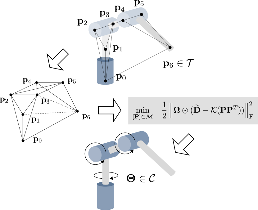
Figure 1: The IK problem consists of finding the joint angles $\boldsymbol{\mathbf{\Theta}}$ that bring the end-effector of a 3-DOF robotic manipulator to its goal position ($\boldsymbol{\mathbf{p}}_{6}$ in the diagram). Our method uses distance information common to all possible IK solutions by defining an incomplete graph whose edges are weighted by known distances. Then, we use low-rank matrix completion to recover the weights corresponding to the unknown edges, solving the IK problem.

II Formulation

A collection of $N$ points rigidly attached to a manipulator with a $K$-dimensional workspace is arranged in a matrix ${\mathbf{P}=[\mathbf{p}_{0},\mathbf{p}_{1},\dots,\mathbf{p}_{N-1}]^{\mathsf{T}}\in\mathbb{R}^{N\times K}}$. All inter-point distances $d_{u,v}$ between $\boldsymbol{\mathbf{p}}_{u}$ and $\boldsymbol{\mathbf{p}}_{v}$ are determined via the Euclidean norm:

$$d_{u,v}=\|\mathbf{p}_{u}-\mathbf{p}_{v}\|_{2}\,.$$

The inner product $\mathbf{X}:=\boldsymbol{\mathbf{P}}\boldsymbol{\mathbf{P}}^{\mathsf{T}}$ is a symmetric positive semidefinite Gram matrix that can be used to compute the full set of squared inter-point distances $d_{u,v}^{2}$,

$$\mathbf{D}=\mathcal{K}(\boldsymbol{\mathbf{X}})=2\ \text{Sym}(\text{diag}\left(\boldsymbol{\mathbf{X}}\right)\boldsymbol{\mathbf{1}}^{\mathsf{T}}-\boldsymbol{\mathbf{X}}),$$ (2)

where $\text{Sym}(\boldsymbol{\mathbf{X}})=\frac{1}{2}(\boldsymbol{\mathbf{X}}+\boldsymbol{\mathbf{X}}^{\mathsf{T}})$ and $\text{diag}\left(\boldsymbol{\mathbf{X}}\right)$ is the vector formed by the main diagonal of $\boldsymbol{\mathbf{X}}$. The resulting matrix $\mathbf{D}$ is known as a Euclidean distance matrix or EDM [7]. Given a full EDM, we can use eigenvalue decomposition to extract the underlying point set $\boldsymbol{\mathbf{P}}$ up to a rigid transformation.

In our point-based kinematics model, a subset of inter-point distances is defined by the manipulator’s rigid link geometry and desired end-effector pose. Joint angle limits define lower bounds on distances between points that share a neighbouring joint. The problem of finding the remaining unknown entries in the resulting partial EDM is known as the EDM completion problem [7, 8]. We denote the $N\times N$ binary matrices that index the locations of all known and lower bounded squared distances of the partial EDM $\tilde{\boldsymbol{\mathbf{D}}}$ as $\Omega$ and $\Psi$ respectively. The problem of finding the missing EDM entries can now be expressed as low-rank matrix completion:

$$\min_{[\boldsymbol{\mathbf{P}}]\in\mathcal{M}} \frac{1}{2}\left\lVert\Omega\odot(\widetilde{\boldsymbol{\mathbf{D}}}-\mathcal{K}(\boldsymbol{\mathbf{P}}\boldsymbol{\mathbf{P}}^{T}))\right\rVert_{F}^{2}$$ (3)

$$+ \frac{1}{2}\left\lVert\mathrm{max}\left\{\Psi\odot(\widetilde{\boldsymbol{\mathbf{D}}}-\mathcal{K}(\boldsymbol{\mathbf{P}}\boldsymbol{\mathbf{P}}^{T})),0\right\}\right\rVert_{F}^{2}\,,$$

where $\odot$ is the element-wise Hadamard product, $\mathrm{max}$ is taken element-wise with 0, and $\mathcal{M}$ is the Riemannian manifold described in Equation 4. By factoring the Gram matrix as $\boldsymbol{\mathbf{X}}=\boldsymbol{\mathbf{P}}\boldsymbol{\mathbf{P}}^{\mathsf{T}}$ and solving for $\boldsymbol{\mathbf{P}}$, we are implicitly constraining the dimensionality of the search space [9], without changing the global minimum [10].

The factorization of the Gram matrix is invariant to orthogonal transformations of the point set $\boldsymbol{\mathbf{P}}\mapsto\boldsymbol{\mathbf{P}}\boldsymbol{\mathbf{Q}}$, where $\boldsymbol{\mathbf{Q}}\in\mathrm{O}(K)$. It follows that the cost function minima are not isolated, which significantly hinders the convergence of second-order optimization methods [11]. Following [6], the local search is constrained to the quotient manifold $\mathcal{M}\equiv\mathbb{R}_{*}^{N\times K}/\mathrm{O}(K)$, which represents the equivalence class

$$[\boldsymbol{\mathbf{P}}]=\left\{\boldsymbol{\mathbf{P}}\boldsymbol{\mathbf{Q}}|\,\boldsymbol{\mathbf{Q}}\in\mathbb{R}^{K\times K}\,,\boldsymbol{\mathbf{Q}}^{T}\boldsymbol{\mathbf{Q}}=\boldsymbol{\mathbf{I}}\right\}.$$ (4)

The geometry of the Riemannian manifold $\mathcal{M}$ isolates minima, and a variety of algorithms can be applied to solve the problem in Equation 3 as an unconstrained Riemannian optimization problem [11].

III Results and Future Work

TABLE I: Experimental results. Each row summarizes 1000 trials. Asterisks ($\ast$) denote the use of angular joint limits.

Robot	Success (%)	Mean Runtime (ms)
planar-10	100	8.1
planar-10*	100	101.9
planar-100	100	166.5
planar-100*	100	1882
spherical-10	100	24.1
spherical-10*	100	58.4
spherical-100	100	641.7
spherical-100*	99.9	9759
UR10	84.2	462.5
UR10*	63.0	350.5

In Table I, we present the results of a simulated evaluation of our method on IK problems for a variety of manipulators. In every instance we formulate and solve the problem in Equation 3 in Python using the pymanopt package on a laptop computer with an Intel^® Core^TM i7-8750H CPU at 2.20 GHz and 16 GB RAM. The IK problems are generated by randomly sampling the configuration space within joint limits, and the problem is initialized using a set of points corresponding to a configuration with joint angles set to $0$. Joint limits are random and symmetric about $0$, with a minimum value of $0.2$ radians. A solution is considered to be correct (successful) if it achieves position and orientation errors lower than $0.01$ meters and $0.01$ radians, respectively.

We begin with 10 and 100 joint manipulators with unit link lengths, denoted by planar-10, spherical-10, planar-100 and spherical-100 in Table I. In all experiments, our method achieves a $100\%$ success rate with mean computation times well under a second. Surprisingly, this result holds even in the somewhat extreme 100-joint examples, albeit with computation time an order of magnitude greater. Next, we introduce joint limits and repeat the experiment, denoting the results with an asterisk ($\ast$). Again, in all cases there is a $100\%$ success rate, with the exception of one failure occurring for spherical-100*. The computation times in the joint-limited cases are generally higher due to the introduction of the second cost term in Equation 3 that enforces lower bounds on a subset of distances. Finally, we take the practical example of the UR10 6-DOF manipulator, where our method succeeds in $84.2\%$ and $63.0\%$ of instances (without and with joint limits, respectively). These success rates are comparable to solvers available in the Kinematics and Dynamics Library [12, Table 1].

These results show promise for distance geometric models in kinematics and motion planning, since low-rank matrix completion and the distance geometry problem in general [8] have strong theoretical underpinnings. In our work, we seek to exploit this perspective to develop new methods for solving and analyzing complex inverse kinematics problems. We are currently experimenting with spherical obstacles, which are easily incorporated into our formulation as points with fixed distances from the robot base and one another, and distances to points on the robot that are bounded from below by each obstacle’s radius.

References

- [1] F. Blanchini, G. Fenu, G. Giordano, and F. A. Pellegrino, “A convex programming approach to the inverse kinematics problem for manipulators under constraints,” European Journal of Control, vol. 33, pp. 11–23, Jan. 2017.
- [2] F. Marić, M. Giamou, S. Khoubyarian, I. Petrović, and J. Kelly, “Inverse kinematics for serial kinematic chains via sum of squares optimization,” in IEEE International Conference on Robotics and Automation, pp. 7101–7107, May/Jun. 2020.
- [3] T. Le Naour, N. Courty, and S. Gibet, “Kinematics in the metric space,” Computers & Graphics, vol. 84, p. 13–23, Nov 2019.
- [4] J. M. Porta, L. Ros, and F. Thomas, “Inverse kinematics by distance matrix completion,” in Proceedings of the12th International Workshop on Computational Kinematics, May 2005.
- [5] J. Porta, L. Ros, F. Thomas, and C. Torras, “A branch-and-prune solver for distance constraints,” IEEE Transactions on Robotics, vol. 21, pp. 176–187, Apr. 2005.
- [6] B. Mishra, G. Meyer, and R. Sepulchre, “Low-rank optimization for distance matrix completion,” IEEE Conference on Decision and Control and European Control Conference, pp. 4455–4460, Dec 2011.
- [7] I. Dokmanic, R. Parhizkar, J. Ranieri, and M. Vetterli, “Euclidean Distance Matrices: Essential Theory, Algorithms and Applications,” IEEE Signal Processing Magazine, vol. 32, pp. 12–30, Nov. 2015.
- [8] L. Liberti, C. Lavor, N. Maculan, and A. Mucherino, “Euclidean distance geometry and applications,” SIAM Rev., vol. 56, pp. 3–69, Jan. 2014.
- [9] S. Burer and R. D. Monteiro, “Local minima and convergence in low-rank semidefinite programming,” Mathematical Programming, vol. 103, p. 427–444, Dec 2004.
- [10] H. Fang and D. P. O’Leary, “Euclidean distance matrix completion problems,” Optimization Methods and Software, vol. 27, pp. 695–717, Oct. 2012.
- [11] P.-A. Absil, R. Mahony, and R. Sepulchre, Optimization Algorithms on Matrix Manifolds. Princeton University Press, 2009.
- [12] P. Beeson and B. Ames, “TRAC-IK: An open-source library for improved solving of generic inverse kinematics,” in IEEE-RAS International Conference on Humanoid Robots, pp. 928–935, IEEE, 2015.