Ab Initio Theory of the Drude Plasma Frequency

Abstract

We derive a theoretical expression to calculate the Drude plasma frequency $\omega_{D}$ based on quantum mechanical time dependent perturbation theory in the long-wavelength regime. We show that in general $\omega_{D}^{2}$ should be replaced by a second rank tensor, the Drude tensor $\bm{\mathcal{D}}$, which we relate to the integral over the Fermi surface of the convective momentum flux tensor divided by the magnitude of the Fermi velocity, and which is amiable to analytical and numerical evaluation. We also obtain an expression in terms of the average inverse mass tensor. For the Sommerfeld’s model of metals our expression yields the ubiquitous plasma frequency $\omega^{2}_{D}=4\pi n_{e}e^{2}/m_{e}$. We compare our expressions to those of other previous theories. The Drude tensor takes into account the geometry of the unit cell and may be calculated from first principles for isotropic as well as anisotropic metallic systems. We present results for the noble metals, Ag, Cu, and Au without stress and subject to isotropic and uniaxial strains, and we compare the results to those available from experiment. We show that within density functional theory, nonlocal potentials are necessary to obtain an accurate Drude tensor.

I Introduction

The Drude theory for the electrical conductivity and the dielectric response of metals has been well known for over a century.Drude (1900a, b) Originally based on the classical kinetic theory of gases, its results survived Sommerfeld’s reformulation in terms of a quantum Fermion gas. They may also be obtained from the local limit of the non-local longitudinal Lindhard dielectric function Ashcroft and Mermin (1976). The purpose of this paper is to generalize the Drude model using a fully quantum mechanical theory for metals and to obtain local expressions that can be directly evaluated for both isotropic and anisotropic systems starting from the Hamiltonian of the system, which may contain many body and non-local interactions.

The Drude theory of metals, put forward back in 1900,Drude (1900a, b) includes among its successes a simple explanation that allows for approximate estimates of properties of metals whose full comprehension required the development of the quantum theory of condensed matter. Drude’s theory of electrical and thermal conductivity was based on the kinetic theory of gases applied to the conduction electrons of the system, while the the core electrons strongly bonded to the atomic nuclei are taken as an inert entity. The precise assumptions of the Drude model are clearly explained in textbooks of solid state theory like Ref. Ashcroft and Mermin, 1976. Drude assumed that the electronic velocity distribution is given by the Maxwell-Boltzmann distribution function, which leads to the wrong result for the specific heat of metals of $3k_{B}/2$, where $k_{b}$ is Boltzmann’s constant. It was Sommerfeld, almost 25 years after the publication of Drude’s results, that recognized the fact that Fermi-Dirac (FD) statistics were required for treating the electron correctly. As it turns out, Sommerfeld’s model is essentially the classical electron gas model used by Drude, but using the FD distribution for the valence electrons. Albeit, one of the first success of Sommerfeld was to obtain the experimental linear behavior of the specific heat of metals.

The Drude model yields the following well known result for the dielectric function $\epsilon(\omega)$ of a metal,Ashcroft and Mermin (1976)

$$\epsilon(\omega)=1-\frac{\omega^{2}_{D}}{\omega^{2}},$$ (1)

where

$$\omega_{D}=\left(\frac{4\pi n_{e}e^{2}}{m_{e}}\right)^{1/2},$$ (2)

is known as the Drude frequency, where $n_{e}$, $-e$ and $m_{e}$ are the number density, charge and free mass of the conduction electrons, and $\omega$ is the frequency of the light that perturbs the electrons. blue In the Drude model $\omega_{D}$ corresponds also to the frequency of the collective plasma oscillations of the system and is usually denoted by $\omega_{p}$ and called the plasma frequency, though this interpretation does not hold in the presence of further screening mechanisims. Although Eq. (1) gives a precise description of the interaction of light with metals for photons with energy below the threshold of electronic interband transitions, a fully quantum-mechanical derivation would justify its successes.

In this article, we derive a closed expression for $\omega_{D}$ based on quantum mechanical time dependent perturbation theory. We show that in general $\omega_{D}^{2}$ should be replaced by a second rank tensor, that we call the Drude tensor $\bm{\mathcal{D}}$, for which we derive a closed expression that is amiable to analytic evaluation in the case of free independent electrons, and to numerical evaluation for ab initio quantum mechanical calculations. The Drude tensor takes into account the geometry of the unit cell and may be calculated from first principles for isotropic as well as anisotropic metallic systems.

The article is organized as follows. In Sec. II, we present the theoretical formalism, showing the main expressions used to calculate the Drude tensor. In Sec. II.1 we derive $\omega_{D}$ within the Drude-Sommerfeld model as a special case of our formalism, and in Sec. II.2 we present the procedure to numerically evaluate the Drude tensor. In Sec. III we present results for the noble metals, Ag, Cu and Au without stress and subject to an isotropic and to an uniaxial strain, and we summarize our findings in Sec. IV.

II Analytic expression for the Drude plasma frequency

In order to derive the analytic expression for the Drude plasma frequency, we assume the electrons may be described through an independent particle approximation, although we do allow for many-body effects through an effective Hamiltonian that depends on all occupied states, as in density functional theory. The electrons interact with an electromagnetic field which we assume is a classical field. Thus we describe quantum mechanical matter interacting with classical fields. We neglect local field and excitonic effects.Onida et al. (2002) We write the one electron Hamiltonian

$$\hat{H}(t)=\hat{H}_{0}+\hat{H}_{I}(t),$$ (3)

as the sum of an unperturbed effective time-independent Hamiltonian $\hat{H}_{0}$ that describes the interaction of an electron with the crystalline lattice and its effective interaction with the other electrons, and an interaction Hamiltonian $\hat{H}_{I}(t)$ that describes the interaction of the electron with a time-dependent electromagnetic field. We describe the state of the system through the one electron density operator $\hat{\rho}$, with which we can calculate the expectation value of any single-particle observable $\hat{\mathcal{O}}$ as $\braket{\hat{\mathcal{O}}}=\mbox{Tr}(\hat{\rho}\hat{\mathcal{O}})$ with Tr denoting the trace. Within the interaction picture the density operator evolves in time due to the interaction Hamiltonian according to

$$i\hbar\frac{d}{dt}\hat{\rho}(t)=[\hat{H}_{I}(t),\hat{\rho}(t)],$$ (4)

while the operators that correspond to all observables evolve through $\hat{H}_{0}$ according to

$$\hat{\mathcal{O}}(t)=\hat{U}^{\dagger}(t)\hat{\mathcal{O}}_{s}(t)\hat{U}(t),$$ (5)

where $\hat{\mathcal{O}}_{s}(t)$ is the same observable in the Schrödinger picture, given by $\hat{\mathcal{O}}(0)$ for operators that do not depend explicitly on time, and

$$\hat{U}(t)=\exp({-i\hat{H}_{0}t/\hbar})$$ (6)

is the non-perturbed unitary time-evolution operator. Assuming the field is turned on adiabatically, we may integrate (4) to yield

$$\hat{\rho}(t)=\hat{\rho}_{0}+\frac{1}{i\hbar}\int_{-\infty}^{t}dt^{\prime}[\hat{H}_{I}(t^{\prime}),\hat{\rho}(t^{\prime})],$$ (7)

where $\hat{\rho}_{0}$ is the unperturbed, time-independent equilibrium density matrix. We look for the standard perturbation series solution, $\hat{\rho}(t)=\hat{\rho}_{0}+\hat{\rho}^{(1)}(t)+\hat{\rho}^{(2)}(t)+\ldots$, where the superscript denotes the order (power) with which each term depends on the perturbation $\hat{H}_{I}(t)$. Since we are interested only in the linear response, we concentrate our attention on the 1-st order term

$$\hat{\rho}^{(1)}(t)=\frac{1}{i\hbar}\int_{-\infty}^{t}dt^{\prime}[\hat{H}_{I}(t^{\prime}),\hat{\rho}_{0}].$$ (8)

We will take our system as a solid described by a non-perturbed periodic Hamiltonian, whose eigenfunctions are Bloch states, $\ket{m\bm{k}}$, characterized by a band index $m$ and a crystal momentum $\bm{k}$. For $\hat{H}_{I}(t)$ we take an interaction with an electromagnetic field with a wavelength much larger than the crystal parameter. Thus, electronic transitions due to this interaction are vertical, i.e., they conserve $\bm{k}$.

Within the dipole approximation, the interaction Hamiltonian in the Length Gauge is given by Anderson et al. (2015)

$$\hat{H}_{I}(t)=e\hat{\bm{r}}(t)\cdot\bm{E}(t),$$ (9)

where $\hat{\bm{r}}(t)=\hat{U}^{\dagger}_{0}(t)\hat{\bm{r}}(0)U(t)$ is the position operator of the electron at time $t$ and $\bm{E}(t)$ the time dependent perturbing classical electric field.

From (8) we obtain the first order density matrix elements between Bloch states

$$\rho^{(1)}_{nm}(\bm{k};t)\equiv\braket{n\bm{k}}{\hat{\rho}^{(1)}(t)}{m\bm{k}} =\frac{1}{i\hbar}\int_{-\infty}^{t}dt^{\prime}\braket{n\bm{k}}{[\hat{H}_{I}(t^{\prime}),\hat{\rho}_{0}]}{m\bm{k}}$$

$$=-\frac{ie}{\hbar}\int_{-\infty}^{t}dt^{\prime}e^{i\omega_{nm}(\bm{k})t^{\prime}}\braket{n\mathbf{k}}{[\hat{\bm{r}}(0),\hat{\rho}_{0}]}{m\bm{k}}\cdot\bm{E}(t^{\prime}),$$ (10)

where $\omega_{nm}(\bm{k})\equiv\omega_{n}(\bm{k})-\omega_{m}(\bm{k})$ and $E_{n}(\bm{k})=\hbar\omega_{n}(\bm{k}))$ are the unperturbed energy eigenvalues corresponding to the stationary Schrödinger’s equation $\hat{H}_{0}\ket{{n\bm{k}}}=E_{n}(\bm{k})\ket{{n\bm{k}}}$. Notice that $\hat{\rho}_{0}$ has matrix elements

$$\braket{n\bm{k}}{\hat{\rho}_{0}}{m\bm{k}}=\delta_{nm}f(E_{n}(\bm{k})),$$ (11)

with $f$ the Fermi-Dirac distribution, which at the temperature $T=0$ becomes

$$f(E_{n}(\bm{k}))=\Theta(E_{F}-E_{n}(\bm{k}))\equiv f_{n}(\bm{k}),$$ (12)

with $E_{F}$ the Fermi energy of the system and $\Theta$ the unit step function. This defines the distributions functions $f_{n}(\bm{k})$ in reciprocal space, one for each band.

It is convenient to represent the position operator in coordinate space $\hat{\bm{r}}(0)\to\bm{r}$, when calculating its interband matrix elements and in reciprocal space $\hat{\bm{r}}(0)\to i\nabla_{\bm{k}}$ when calculating its intraband matrix elements, so that following Ref. Aversa and Sipe, 1995-11-15, we can readily show that

$$\braket{n\bm{k}}{[\hat{\mathbf{r}},\hat{\rho}_{0}]}{m\bm{k}}=f_{mn}(\bm{k})\bm{r}_{nm}(\bm{k})+i\delta_{nm}\nabla_{\bm{k}}f_{n}(\bm{k}),$$ (13)

where $f_{nm}(\bm{k})=f_{n}(\bm{k})-f_{m}(\bm{k})$ and $\bm{r}_{nm}(\bm{k})=\braket{n\bm{k}}{\bm{r}}{m\bm{k}}$. Notice that $f_{nm}(\bm{k})=0$ if $n=m$. The well-known commutator

$$\hat{\bm{v}}=\hat{\dot{\bm{r}}}=\frac{1}{i\hbar}[\hat{\bm{r}},\hat{H}_{0}],$$ (14)

allows us to write the interband matrix element as

$$\bm{r}_{nm}(\bm{k})=\frac{\bm{v}_{nm}(\bm{k})}{i\omega_{nm}(\bm{k})}\quad(n\neq m),$$ (15)

where $\hat{\bm{v}}$ is the velocity operator related to the momentum operator by $\hat{\bm{p}}=m_{e}\hat{\bm{v}}$.

To obtain the optical linear response we look for the expectation value of the macroscopic polarization density $\bm{P}$, whose time derivative yields the current density, i.e., the expectation value of the current operator. Thus,

$$\frac{\partial}{\partial t}\bm{P}=-\frac{e}{\Omega}\mbox{Tr}\,({\hat{\rho}^{(1)}}(t)\hat{{\mathbf{v}}}(t)),$$ (16)

with $\Omega$ the volume of the unit cell. Assuming an harmonic perturbation $\bm{E}(t)=\bm{E}(\omega)e^{-i\omega t}$, we obtain the tensorial relation

$$P^{a}(\omega)=\chi^{ab}(\omega)E^{b}(\omega),$$ (17)

where $\chi^{ab}(\omega)$ is the linear susceptibility response tensor, where the superscripts $\mathrm{a,b}$ denote Cartesian components, and we use Einstein convention for repeated indices. Using Eqs. (10)-(17), we obtain

$$\chi^{ab}(\omega) =\frac{ie^{2}}{\hbar\omega}\sum_{mn}\int_{\mathrm{BZ}}\frac{d^{3}k}{8\pi^{3}}v^{a}_{mn}(\bm{k})\left(\frac{f_{mn}(\bm{k})r^{b}_{nm}(\bm{k})+i\delta_{nm}\partial_{k^{b}}f_{n}(\bm{k})}{\omega_{nm}(\mathbf{k})-\omega}\right)$$

$$=\chi_{e}^{ab}(\omega)+\chi_{i}^{ab}(\omega),$$ (18)

where the sums over band indices and over the wavevector correspond to the trace and the latter was replaced by the usual integral over the first Brillouin zone (BZ), we defined $\partial_{k^{b}}=\partial/\partial k^{b}$ to simplify our notation, and we identified the interband $\chi_{e}^{ab}(\omega)$ and intraband $\chi_{i}^{ab}(\omega)$ contributions to the susceptibility as those that contain the first and second terms in the numerator of Eq. (II), those which contain the factor $f_{nm}(\bm{k})$ and the Kronecker’s delta $\delta_{nm}$ respectively. Using Eq. (15) we write the interband contribution as

$$\chi_{e}^{ab}(\omega) =\frac{e^{2}}{\hbar\omega}\sum_{mn}\int_{\mathrm{BZ}}\frac{d^{3}k}{8\pi^{3}}f_{mn}(\bm{k})\omega_{nm}(\bm{k})\left(\frac{r^{a}_{mn}(\bm{k})r^{b}_{nm}(\bm{k})}{\omega_{nm}(\bm{k})-\omega}\right).$$ (19)

The intraband contribution is

$$\chi_{i}^{ab}(\omega) =\frac{ie^{2}}{\hbar\omega}\sum_{mn}\int_{\mathrm{BZ}}\frac{d^{3}k}{8\pi^{3}}v^{a}_{mn}(\bm{k})\left(\frac{i\delta_{nm}\partial_{k^{b}}f_{n}(\bm{k})}{\omega_{nm}(\bm{k})-\omega}\right)=\frac{e^{2}}{\hbar\omega^{2}}\sum_{n}\int_{\mathrm{BZ}}\frac{d\bm{k}}{8\pi^{3}}v^{a}_{n}(\bm{k})\partial_{k^{b}}f_{n}(\bm{k}),$$ (20)

where we denote $v^{a}_{nn}(\bm{k})$ as $v^{a}_{n}(\bm{k})$, the electron’s velocity for the $n$-th band at point $\bm{k}$ of the Brillouin zone. We recognize $\chi_{e}^{ab}(\omega)$ as the well known linear susceptibility amply discussed in the scientific literature as well as in textbooks of physics; in the rest of the article, we only devote our attention to $\chi_{i}^{ab}(\omega)$, that as we see now, leads to a closed and computationally amenable expression for the Drude frequency.

We rewrite Eq. (20) as

$$\chi_{i}^{ab}(\omega) =-\frac{1}{4\pi\omega^{2}}{\mathcal{D}}^{ab},$$ (21)

where we define the Drude tensor as

$${\mathcal{D}}^{ab} =-\frac{4\pi e^{2}}{\hbar}\sum_{n}\int_{\mathrm{BZ}}\frac{d^{3}k}{8\pi^{3}}v^{a}_{n}(\bm{k})\partial_{k^{b}}f_{n}(\bm{k})$$

$$=\frac{e^{2}}{2\pi^{2}}\sum_{n}\int_{\mathrm{BZ}}d^{3}k\,v^{a}_{n}(\bm{k})v^{b}_{n}(\bm{k})\delta(E_{F}-E_{n}(\bm{k})).$$ (22)

Here, we used Eq. (12) for $f_{n}(\bm{k})$, employed the derivative of the Heaviside step function with respect to its argument, $d\Theta(x)/dx=\delta(x)$, and identified the velocity of the electron in the $n$-th band from the dispersion of the corresponding energy $\nabla_{\bm{k}}E_{n}(\bm{k})=\hbar\bm{v}_{n}(\bm{k})$. blue Notice that the expression in Eq. (6) of Ref. Maksimov et al., 1988 corresponds to $\mbox{Tr}\,{\bm{\mathcal{D}}}/3$ , as it relates to an isotropic system.

For any two scalar valued functions $F(\bm{k})$ and $G(\bm{k})$ of the crystal momentum $\bm{k}$, we can evaluateHörmander (1990)

$$\int_{\mathrm{BZ}}d^{3}k\,F(\bm{k})\delta\left(G(\bm{k})\right)=\int_{S}d^{2}\sigma_{\bm{k}}\,\frac{F(\bm{k})}{|\nabla_{\bm{k}}G(\bm{k})|},$$ (23)

which takes us from an integration over the first Brillouin zone with a Dirac’s delta function $\delta(G(\bm{k}))$ to a surface integral over that surface $S$ within the first Brillouin zone for which $G(\bm{k})=0$, with $d^{2}\sigma_{\bm{k}}$ the differential element of area in reciprocal space. Notice that $S$ may have zero, one or more connected components, so that we interpret the surface integral as implying a sum over all of them. Applying this result to Eq. (II) we obtain

$${\mathcal{D}}^{ab} =\frac{e^{2}}{2\pi^{2}}s\sum_{n}\int_{S_{n}}d^{2}\sigma_{\bm{k}}\frac{v^{a}_{n}(\bm{k})v^{b}_{n}(\bm{k})}{|\nabla_{\bm{k}}(E_{F}-E_{n}(\bm{k}))|}$$

$$=\frac{e^{2}}{2\pi^{2}\hbar}s\sum_{n}\int_{S_{n}}d^{2}\sigma_{\bm{k}}\frac{v^{a}_{n}(\bm{k})v^{b}_{n}(\bm{k})}{v_{n}(\bm{k})},$$ (24)

where $S_{n}$ is the contribution of the $n$-th band to the Fermi Surface (FS), defined by those Bloch vectors $\bm{k}$ for which $E_{n}(\bm{k})=E_{F}$. This is the main result of our paper, as it allows the calculation of the Drude tensor, the intraband susceptibility and its contribution to the dielectric response for any metal from its electronic structure. Notice that $\mathcal{D}^{ab}$ is proportional to the integral over the Fermi surface of blue the convective contribution to the momentum flux tensor $m\bm{v}_{n}\bm{v}_{n}$, with components $mv_{n}^{a}v_{n}^{b}$ divided by the magnitude of the velocity $v_{n}$, summed over the conduction bands and integrated over the Fermi surface. We have included in Eq. (II) a spin-degeneracy factor $s$ which allows us to ignore the spin in the state labels $n$ for those systems that are spin-degenerate. Thus, we take $s=1$ if the band index includes the spin, as would be the case when the spin-orbit coupling is included in the calculation, and $s=2$ when the spin is not explicitly included.

For a semiconductor there are no bands that cross the Fermi Energy, and then the Drude tensor is identically zero, or in other words, there is no intraband contribution to the susceptibility. For a metal, there is at least one band that crosses the $E_{F}$, yielding a finite intraband contribution. The intraband dielectric tensor may be written written as

$$\epsilon_{i}^{ab}=\delta_{ab}+4\pi\chi_{i}^{ab}=\delta_{ab}-\frac{{\mathcal{D}}^{ab}}{\omega^{2}},$$ (25)

giving the characteristic $1/\omega^{2}$ divergence as $\omega\to 0$ for the dielectric function of metals. Notice that ${\mathcal{D}}^{ab}$ has units of frequency squared and that it would agree with Eq. (1) for a Drude model if we identify $\mathcal{D}^{ab}=\omega_{D}^{2}\delta_{ab}$ with $\omega_{D}$ given by Eq. (2). Thus, the interband contribution to the dielectric response given by Eqs. (II) and (25) can be seen a generalization of the Drude model. blue However, we should remark that there are further screening processes that may shift the actual plasma frequencies away from the Drude frequency, as illustrated below; the plasma frequencies are given by the singluarities of the full dielectric response, and not only of its Drude contribution. Furthermore, our dielectric response has an explicit tensorial character in contrast to that found in standard textbooks, which always describe a scalar dielectric response. The symmetry of the system determines which components of $\mathcal{D}^{ab}$ are blue non-null and how they relate among themselves.

We may write the Drude tensor in a more familiar way by integrating by parts the first line of Eq. (II), to obtain

$$\mathcal{D}^{ab} =\frac{4\pi e^{2}}{\hbar}\sum_{n}\int_{\mathrm{BZ}}\frac{d^{3}k}{8\pi^{3}}f_{n}(\bm{k})\partial_{k^{b}}v^{a}_{n}(\bm{k}),$$ (26)

and identify

$$\partial_{k^{b}}v^{a}_{n}(\bm{k})=\hbar(m^{*}_{n}(\bm{k}))^{-1}_{ab},$$ (27)

from Ref. Cabellos et al., 2009, where $\bm{m}^{*}_{n}(\bm{k})$ is the effective mass tensor. Then

$$\mathcal{D}^{ab} =4\pi e^{2}\sum_{n}\int_{\mathrm{BZ}}\frac{d^{3}k}{8\pi^{3}}f_{n}(\bm{k})({m^{*}_{n}(\bm{k})})^{-1}_{ab}=4\pi n_{e}e^{2}\braket{(m^{*})^{-1}_{ab}},$$ (28)

where the sum may be restricted to the conduction bands. This result is similar to the usual Drude formula with $n_{e}$ the number density of conduction electrons but with the inverse electronic mass $1/m_{e}$ replaced by an average $\braket{(\bm{m}*)^{-1}}$ of the inverse effective mass tensor over the occupied states of the conduction bands. Although this result looks appealing, it hides the fact that only the electrons at the Fermi surface do contribute to the dynamics and the response of the system. Furthermore, the numerical integration over the full BZ in Eq. (28) would require a larger grid $\{\bm{k}_{\alpha}\}$ of k-points and would be more costly to evaluate than the numerical integral (II) only over those $\bm{k}$ points close to the Fermi surface (see Sec. II.2). Finally, evaluation of the inverse mass tensor in Eq. (28) requires a larger computational cost and has a larger numerical uncertainty than the evaluation of the velocity matrix elements in Eq. (II).

II.1 Ideal Metal

Within the Sommerfeld theory of metals the conduction electrons have the dispersion relation of free electrons $E=\hbar^{2}k^{2}/2m_{e}$ and fill up a Fermi sphere of radius $k_{F}$, related to the number density $n_{e}$ of conduction electrons throughAshcroft and Mermin (1976) $n_{e}=k_{F}^{3}/3\pi^{2}$. blue The Fermi velocity is $v_{F}=\hbar k_{F}/m_{e}$. Due to the spherical symmetry, ${\mathcal{D}}^{ab}=0$ for $a\neq b$, and ${\mathcal{D}}^{xx}={\mathcal{D}}^{yy}={\mathcal{D}}^{zz}=\mathcal{D}^{aa}/3\equiv\omega_{D}^{2}$, Then, from Eq. (II)

$$\omega^{2}_{D}=\frac{1}{3}\frac{e^{2}}{2\pi^{2}\hbar}s\int k_{F}^{2}d^{2}\Omega\,v_{F}=4\pi\frac{k_{F}^{3}}{3\pi^{2}}\frac{e^{2}}{m_{e}}=\frac{4\pi n_{e}e^{2}}{m_{e}},$$ (29)

where we wrote $d^{2}\sigma_{\bm{k}}=k_{F}^{2}d^{2}\Omega$, with $d^{2}\Omega$ the differential element of solid angle. Thus $\omega_{D}$ is the well known Drude value for the plasma frequency, however derived from Eq. (II) which comes from a purely quantum mechanical approach within time-dependent perturbation theory, instead of the text-book derivation from the phenomenological model of Drude. Curiously, $\omega_{D}^{2}$ is proportional to the number density $n_{e}$ of conduction electrons, although only those electrons at the Fermi surface contribute to the integral in Eq. (II).

II.2 Realistic metal

Eq. (II) is an elegant expression of the Drude tensor in terms of an integral over the Fermi surface of a tensor formed by blue products of components of the velocity divided by its magnitude $v_{n}^{a}v_{n}^{b}/v_{n}$. However, for actual applications to realistic models it is convenient to return to a volume integral. To that end, we realize that for any function $g(\bm{k})$ we can write

$$\int_{S_{n}}d^{2}\sigma_{\bm{k}}\,g(\bm{k})=\int_{\mathrm{BZ}}d^{3}k\,g(\bm{k})|\nabla f_{n}(\bm{k})|,$$ (30)

as can be immediately verified using Eqs. (12) and (23). Thus, we write Eq. (II) as

$${\mathcal{D}}^{ab}=\frac{e^{2}}{2\pi^{2}\hbar}s\sum_{n}\int_{\mathrm{BZ}}d^{3}k|\nabla_{\bm{k}}f_{n}(\bm{k})|\frac{v^{a}_{n}(\bm{k})v^{b}_{n}(\bm{k})}{v_{n}(\bm{k})}.$$ (31)

To carry out the integration numerically, we generate a regular grid $\{\bm{k}_{\alpha}\}$ of points inside the Irreducible Brillouin Zone that corresponds to the crystallographic group of the metal under study, numbered by a discrete set of indices $\alpha$. Then, we approximate $\nabla_{\bm{k}}f_{n}(\bm{k})|_{\bm{k}_{\alpha}}$ through a finite difference approximation. As the resulting numerical gradient of the Fermi-Dirac distribution would be null away from the Fermi surface, we can refine our grid in its vicinity without a substantial increase in the computational cost, where $E_{F}$ is obtained by using the prescription given in Ref. Burdick, 1962. For those points where the numerical gradient is non-null we evaluate the components of the velocity. Then we can replace the integral by a Riemann sum and write

$${\mathcal{D}}^{ab}=\frac{e^{2}}{2\pi^{2}\hbar}s(\Delta k)^{3}\sum_{n}\sum_{\alpha}|\nabla f_{n}(\bm{k}_{\alpha})|\frac{v^{a}_{n}(\bm{k}_{\alpha})v^{b}_{n}(\bm{k}_{\alpha})}{v_{n}(\bm{k}_{\alpha})},$$ (32)

where $\Delta k$ is the distance between neighbor vectors $\bm{k}_{\alpha}$ in our grid.

III Results

We present results for the three noble metals, Ag, Au and Cu. However, we do so with more detail for Ag, for which there is a recent accurate experimental measurement for the Drude frequency $\hbar\omega_{D}=8.9\pm 0.2$ eV.Yang et al. (2015) Furthermore, we also consider the case of a metal under applied stresses consisting of an isotropic and an anisotropic uniaxial strain. For the isotropic deformation we simply modify the lattice constant $a=(1+\gamma)a_{0}$ with respect to the equilibrium lattice constant $a_{0}$ in the absence of stress. For the anisotropic deformation we keep the original volume of the FCC unit cell, and deform it by stretching along the $z$ direction $a_{z}=(1+\gamma)a_{0}$ while shrinking it along the $x$ and $y$ directions, $a_{x}=a_{y}=a_{\parallel}=a_{0}/\sqrt{1+\gamma}$, thus converting the FCC-lattice into a BCT-lattice. We allow the expansion factor $\gamma$ to take negative as well as positive values. Given the symmetry of these systems, we expect $D^{ab}=0$ if $a\neq b$, $D^{xx}=D^{yy}\equiv D^{\parallel}$ in the uniaxial case and $D^{ab}\equiv D^{\mathrm{iso}}\delta_{ab}$ in the isotropic case. Therefore, we define the Drude frequencies

$$\omega^{\mathrm{iso}}_{D} =\sqrt{\mathcal{D}^{\mathrm{iso}}} \quad\mathrm{isotropic},$$ (33)

$$\omega^{\parallel}_{D} =\sqrt{{\mathcal{D}}^{\parallel}} \quad\mathrm{anisotropic},$$

$$\omega^{z}_{D} =\sqrt{{\mathcal{D}}^{z}} \quad\mathrm{anisotropic}.$$

The self-consistent ground state and the Kohn-Sham states were calculated in the DFT-LDA framework using the plane-wave ABINIT code.abi We used Troullier-Martins pseudopotentialsTroullier and Martins (1991) that are fully separable nonlocal pseudopotentials in the Kleinman-Bylander form.Kleinman and Bylander (1982) We use $a_{0}=4.0853$ Å, for Ag, $a_{0}=3.6149$ Å, for Cu, and $a_{0}=4.0782$ Å, for Au, all taken from Ref. uce, . For the noble metals only the 6th-band is partially filled and thus crossed by the Fermi Energy, therefore in Eq. (32) the sum over $n$ picks up only the value $n=6$. Finally, the number of $\bm{k}$-points used for the calculation was around $\sim 100,000$.

III.1 Ag

In Fig. 1 we show $\omega^{\mathrm{iso}}_{D}(\gamma)$, $\omega^{\parallel}_{D}(\gamma)$ and $\omega^{z}_{D}(\gamma)$ as a function of the corresponding deformation $\gamma$ of the unit cell. First, we point out that the three calculations agree among themselves in the limit of no deformation $\gamma=0$, and that the resulting value $\hbar\omega_{D}(\gamma=0)=9.38\mathrm{eV}$ is only  5% off from the experimental value $\hbar\omega_{D}=8.9\pm 0.2\mathrm{eV}$ Yang et al. (2015). The values chosen for the compressive ($\gamma<0$) and expansive ($\gamma>0$) deformations are experimentally feasible,Akahamaa and Kawamura (2004) and although small, show a sizable difference for the anisotropic deformation values of $\omega^{\parallel}_{D}$ and $\omega^{z}_{D}$. However, for the isotropic deformation $\omega^{\mathrm{i}so}_{D}$ does not deviate that much from its undeformed value.

We notice that for very small values of $\gamma$ both isotropic and anisotropic results are almost the same, but as $\gamma$ deviates away from 0, sizable changes are seen. The isotropic result $\omega^{\mathrm{iso}}_{D}(\gamma)$ is relatively flat with values between 9.2 and 9.4 eV. On the other hand, the anisotropic deformation gives an $\omega^{\parallel,z}_{D}(\gamma)$ that decreases as $a_{z}$ is shortened. Also, as $a_{z}$ is stretched, for values of $\gamma\leq 0.3\%$, both $\omega^{\parallel}_{D}(\gamma)$ and $\omega^{z}_{D}(\gamma)$ increase and show similar values, whereas for larger values of $\gamma\geq 0.3\%$, $\omega^{\parallel}_{D}(\gamma)$ continues increasing while $\omega^{z}_{D}(\gamma)$ reaches a maximum and starts decreasing. Our results show some oscillations that are due to our approximating a surface integral through a volume integral represented as a sum over a discrete grid. As we deform the system, the true Fermi surface sweeps across the grid points, giving rise to the oscillations which may be interpreted as indicative of the accuracy of our calculation. We expect that they could be somewhat filtered away by approximating the gradient with a higher order finite differences formula. It is worth mentioning that, as explained in Ref. Yang et al., 2015, the experimental error in $\hbar\omega_{D}$ of $\sim 0.2$ eV will make our predictions easily verifiable.

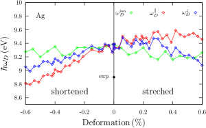
Figure 1: (Color Online) Drude $\hbar\omega_{D}$ vs. the deformation of the unit cell for Ag.

An important theoretical point in our formulation is the fact that the expression for the Drude tensor, Eq. (32), depends on matrix elements of the velocity operator which we calculated according to Eq. (14). We used a non local unperturbed Hamiltonian

$$\hat{H}_{0}=\frac{\hat{p}^{2}}{2m}+\hat{V}^{\mathrm{l}}+\hat{V}^{\mathrm{nl}},$$ (34)

where $\hat{V}^{\mathrm{l}}$ is the local potential characterized by the function $V^{\mathrm{l}}(\bm{r})$, and $\hat{V}^{\mathrm{nl}}$ is the nonlocal potential characterized by the kernel $V^{\mathrm{nl}}(\bm{r},\bm{r}^{\prime})$. The Schrödinger equation reads

$$\left(-\frac{\hbar^{2}}{2m}\nabla^{2}+V^{\mathrm{l}}(\bm{r})\right)\psi_{n\bm{k}}(\bm{r})+\int d^{3}r^{\prime}\,\hat{V}^{\mathrm{nl}}(\bm{r},\bm{r}^{\prime})\psi_{n\bm{k}}(\bm{r}^{\prime})=E_{n}(\bm{k})\psi_{n\bm{k}}(\bm{r}),$$ (35)

The nonlocal potential is more important for metals, where the orbitals of the conduction electrons are farther away form the nucleus, than for semiconductors, for which they are usually much closer. Therefore, we show that it is very important for our calculation to include the nonlocal contribution to the velocity $\bm{v}_{n}(\bm{k})$. In our case, this was carried out using the DP code.Olevano et al. In Fig. 2 we show $\omega^{\parallel}_{D}(\gamma)$, with and without the contribution of the nonlocal potential $V^{\mathrm{nl}}(\bm{r},\bm{r}^{\prime})$. We see that it is mandatory to include it, otherwise the value of $\omega^{\|}_{D}$ would be heavily underestimated. Similar results are found for $\omega^{\mathrm{iso}}_{D}$ and $\omega^{z}_{D}$. We remark that the non-locality of the Hamiltonian arises from its being an effective one particle effective Hamiltonian for a many-body system.Pulci et al. (1998)

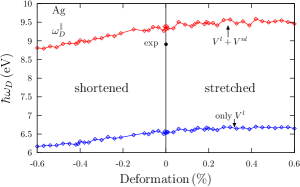
Figure 2: (Color Online) Drude $\hbar\omega^{\parallel}_{D}$ vs. the deformation $\gamma$ of the unit cell for Ag with and without the nonlocal potential $\hat{V}^{nl}(\bm{r},\bm{r}^{\prime})$.

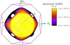
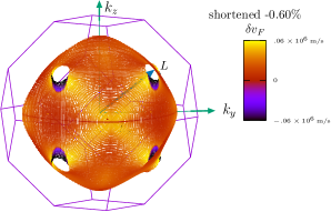
Figure 3: (Color Online) $|v_{x,F}|$ (top-left), $|v_{z,F}|$ (top-right) and $\delta v_{F}=v_{z,F}(k_{x},k_{y},k_{z})-v_{x,F}(k_{z},k_{y},k_{x})$ (bottom) at the Fermi Surface for Ag with an anisotropic deformation of $\gamma=-0.6\%$. The necks are centered at the $L$ point. See the text for details.

As explained in Sec. II.2, the numerical calculation of Eq. (32) requires the $\bm{k}_{\alpha}$-points at the FS as well as the velocities evaluated at each of these points. In Fig. 3 we show the FS and the Fermi velocity for an anisotropic deformation $\gamma=-0.6\%$ as a illustrative example. We see that blue the velocities are of the order expected from the Sommerfeld model,Ashcroft and Mermin (1976) $\sim 10^{6}$ m/s. The system is symmetric under reflections on the Cartesian planes and under an inversion around the origin. As the unit cell has the same lattice parameter along $x$ and $y$, that $v^{x}_{F}$ and $v^{y}_{F}$ agree after a rotation of the system by 90 degrees in the plane, equivalent to an exchange $k_{x}\leftrightarrow k_{y}$, but they differ from $v^{z}_{F}$ after a rotation by 90 degrees around the $y$ axis due to the uniaxial strain. Fig. 3 shows that in this case the $x-z$ anisotropy $\delta v_{F}=v^{z}_{F}(k_{x},k_{y},k_{z})-v^{x}_{F}(k_{z},k_{y},k_{x})$ is of the order of a few percent. It is quite interesting to see that around the FS necks, centered at the $L$-point the velocity is not uniform.

blue In order to illustrate the difference remarked previously between the Drude and the plasma frequencies, in Fig. 4 we show the dielectric function of unstrained Ag incorporating both its interband and its intraband contributions. The intraband contribution has a peak due to d-sp transitions below the Drude frequency, and this pulls the dielectric function upwards, which thus, crosses zero at the plasmon energy $\hbar\omega_{p}=3.95\,\mbox{eV}/\hbar$, much lower than the Drude result $\hbar\omega_{D}=9.36\,\mbox{eV}$. To obtain this result we accounted for the difference in energy of the excited bands as compared to the DFT-LDA prediction, by using the GW formalism within the scissors operator approximation, as described in Ref. Cabellos et al., 2009.

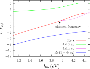
Figure 4: blue Full dielectric function of unstrained Ag and its interband and intraband contributions. Notice that the plasma frequency, given by its zero, differs significantly from the Drude frequency.

III.2 Cu and Au

In Fig. 5 we show $\omega^{\mathrm{iso}}_{D}(\gamma)$, $\omega^{\parallel}_{D}(\gamma)$ and $\omega^{z}_{D}(\gamma)$ as a function of the corresponding deformation $\gamma$ of the unit cell for Cu and Au. As for Ag, we notice that for very small values of $\gamma$ both isotropic and anisotropic results are almost the same, but as $\gamma$ deviates away from 0, sizable changes are seen. The qualitative behavior of $\omega_{D}$ for Cu and Au is very similar to that of Ag, and thus we do not describe it again for briefness sake. The theoretical values of $\hbar\omega_{D}(\gamma=0)=8.97$ eV for Cu and $\hbar\omega_{D}(\gamma=0)=8.59$ eV for Au for the unstrained case are close to the experimental results reported in Ref. pla, and shown in Table. (1). However, the experimental values, except that of Ag in Ref. Yang et al., 2015, have been reported without stating the experimental uncertainty, and there are some noticeable differences among various experimental results, so there is definitely a need for more precise experimental measurements of the Drude plasma frequency for Cu and Au. However, we point out that our results are well within the dispersion of the available experiments.

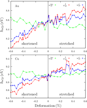
Figure 5: (Color Online) Drude $\hbar\omega_{D}$ vs. the deformation of the unit cell for Au and Cu.

blue Finally, in Fig. 6 we illustrate the convergence of our results as the number of grid points in the vicinity of the Fermi surface is increased. It may be appreciated that our results are adequately converged.

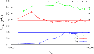
Figure 6: blue Drude $\hbar\omega_{D}$ of unstrained Ag, Cu and Au as a function of the number of grid points in the vicinity of the Fermi surface employed in its calculation.

III.3 Previous Work

In Ref.  Marini et al., 2001, the Drude plasma frequency was obtained through an expression derived from the intraband part of the dielectric function, in the same spirit as we have done here, but using a non-local longitudinal susceptibility that depends on the value of a wavevector $\bm{q}$, for which the limit $q\to 0$ had to be numerically approximated, being fixed at a rather arbitrary chosen small value $|\bm{q}|=0.005$ a.u. Furthermore, a fictitious finite electronic temperature $T$ was used to smooth out the Fermi-Dirac distribution function. As we show in appendix A, taking the actual limits $q\to 0$ and $T\to 0$ of their expression, we recover our Eq. (II). However, in their approach, different directions of $\bm{q}$ should be used to obtain all the components of the tensor $\mathcal{D}^{ab}$ while our approach does not require extraneous parameters. The results of Refs. Marini et al., 2001 and Marini et al., 2002, give $\hbar\omega_{D}=9.27$ for Cu and $\hbar\omega_{D}=9.48$ eV for Ag, respectively, that are not far from our values, as shown in Table  (1).

Also, in Ref. Maksimov et al., 1988, using a similar procedure to that of Ref. Marini et al., 2001, the Drude plasma frequency was obtained by taking the limit $q\to 0$ analytically. However, the resulting expression is valid only for isotropic systems, for which it agrees with $\mathcal{D}^{\mathrm{iso}}$ as derived from our Eq. (II). Finally, the expression for $\mathcal{D}^{\mathrm{iso}}$, as derived in Ref. Maksimov et al., 1988, was used in Ref. Pedersen et al., 2009 for the study of tin and in Ref. Jung and Pedersen, 2013 the study of of heavily doped semiconductors.

	Experimental	Theoretical
		This work	Others
Ag	8.9$\pm$0.2Yang et al. (2015), 8.6Hooper and Sambles (2002), 9.013Ordal et al. (1985), 9.04Zeman and Schatz (1987), 9.6Blaber et al. (2009)	9.38	9.48Marini et al. (2002)
Cu	7.389Ordal et al. (1985), 8.76Zeman and Schatz (1987)	8.97	9.27Marini et al. (2001)
Au	7.9Kreiter et al. (2002), 8.55Blaber et al. (2009), 8.89Zeman and Schatz (1987), 9Berciaud et al. (2005), 8.951Grady et al. (2004), 9.026Ordal et al. (1985)	8.59	-

Table 1: Experimental and theoretical values of $\hbar\omega_{D}$ in eV for Ag, Cu, and Au in the absence of strain.

blue Finally, in Ref. Cazzaniga et al., 2010 the reciprocal-vector-dependent intraband contribution to the dielectric response was obtained through an analytical expansion of several terms to low order in the small optical wavenumber. Their expressions could be used to include local field corrections, and they were applied to RPA-like calculations of the response of Fe and Mg, obtainaining good agreement with experiment. They emphasized, as we did above, the importance of using non-local pseudopotentials. Their formalism for the dielectric function is similar to ours, though we did not require an expansion for the long wavelength case and they did not identify explicitly an expression for the Drude tensor.

IV Conclusions

We have shown that the well known Drude plasma frequency, $\omega_{D}^{2}$, should be replaced by the Drude tensor $\bm{\mathcal{D}}$, for which we have derived a closed theoretical expression based on quantum mechanical time dependent perturbation theory. The expression for $\bm{\mathcal{D}}$ as the integral over the Fermi surface of a tensor built up from matrix elements of the velocity operator is amiable to analytic and numerical evaluation. Using the Sommerfeld model for metals, we showed that $\bm{\mathcal{D}}$ leads to the well known result of $\omega^{2}_{D}=4\pi ne^{2}/m_{e}$. We calculated $\bm{\mathcal{D}}$ for the noble metals, and we described the results for Ag in depth, since there is a recent precise result of $\omega_{D}=8.9\pm 0.2$ eV.Yang et al. (2015) We showed that non-local potentials ought to be used when calculating the velocity matrix elements in order to obtain an accurate result. In summary, the results of $\omega_{D}$ for Cu, Ag and Au for the undeformed unit cell with a lattice constant taken from measurements at room temperature, coincide rather well with the experimental results. We have made predictions for the noble metals subject to an isotropic and to an uniaxial stress that could be experimentally verified.

Funding

B.S.M. acknowledges the support from CONACyT through grant A1-S-9410. W.L.M. acknowledges the support from DGAPA-UNAM under grant IN111119.

Disclosures

The authors declare no conflicts of interest.

Appendix A Comparison with Marini et al. Marini et al. (2001)

Eq. (17) of Marini et al.Marini et al. (2001), derived from the local limit of the longitudinal non-local susceptibility, reads

$$\hbar^{2}\omega^{2}_{D} =\lim_{\bm{q}\to 0}\frac{8\pi e^{2}}{|\bm{q}|^{2}}\int\frac{d^{3}k}{8\pi^{3}}\left(f_{n}(\bm{k}-\bm{q})-f_{n}(\bm{k})\right)\Theta\left(f_{n}(\bm{k}-\bm{q})-f_{n}(\bm{k})\right)$$

$$\times\left|\langle n\bm{k}|e^{i\bm{q}\cdot\bm{r}}|{n\bm{k}-\bm{q}}\rangle\right|^{2}\left(E_{n}(\bm{k}-\bm{q})-E_{n}(\bm{k})\right),$$ (36)

where $\bm{q}$ is the wavevector of the field. We use $\bm{k}\cdot\bm{p}$ theory to approximate this expression for small $\bm{q}$ using the following results:

$$E_{n}(\bm{k}+\bm{q}) =E_{n}(\bm{k})+\hbar\bm{q}\cdot\bm{v}_{nn}(\bm{k})+{\mathcal{O}}(q^{2})$$

$$\ket{n\bm{k}+\bm{q}} =e^{i\bm{q}\cdot\bm{r}}\left(\ket{n\bm{k}}+\ket{n\bm{k}}^{(1)}+{\mathcal{O}}(q^{2})\right)$$

$$\ket{n\bm{k}}^{(1)} =\hbar\sum_{m\neq n}\frac{\bm{q}\cdot\bm{v}_{mn}(\bm{k})}{E_{n}-E_{m}}\ket{m\bm{k}}.$$ (37)

Then, to first order in $\bm{q}$, we obtain,

$$\ket{n\bm{k}+\bm{q}} =(1+i\bm{q}\cdot\bm{r})\left(\ket{n\bm{k}}+\ket{n\bm{k}}^{(1)}+{\mathcal{O}}(q^{2})\right)$$

$$\approx\ket{n\bm{k}}+i\bm{q}\cdot\bm{r}\ket{n\bm{k}}+\ket{n\bm{k}}^{(1)},$$ (38)

$$\braket{n\bm{k}}{e^{i\bm{q}\cdot\bm{r}}}{{n\bm{k}-\bm{q}}} \approx\bra{n\bm{k}}\left(1+i\bm{q}\cdot\bm{r})(\ket{n\bm{k}}-i\bm{q}\cdot\bm{r}\ket{n\bm{k}}+\ket{n\bm{k}}^{(1)}\right)$$

$$=1+\braket{n\bm{k}}{n\bm{k}}^{(1)}$$

$$=1+\hbar\sum_{m\neq n}\frac{\bm{q}\cdot\bm{v}_{mn}(\bm{k})}{E_{n}-E_{m}}\braket{n\bm{k}}{m\bm{k}}=1+\hbar\sum_{m\neq n}\frac{\bm{q}\cdot\bm{v}_{mn}(\bm{k})}{E_{n}-E_{m}}\delta_{nm}=1,$$ (39)

and

$$E_{n}(\bm{k})-E_{n}(\bm{k}-\bm{q})\approx\hbar\bm{q}\cdot\bm{v}_{nn}(\bm{k}).$$ (40)

With these results, and denoting $\bm{v}_{nn}(\bm{k})$ as $\bm{v}_{n}(\bm{k})$, Eq. (A) may be written as

$$\hbar^{2}\omega^{2}_{D} =\lim_{\bm{q}\to 0}\frac{8\pi e^{2}}{|\bm{q}|^{2}}\int\frac{d^{3}k}{8\pi^{3}}\hbar\bm{q}\cdot\bm{v}_{n}(\bm{k})\delta(E_{F}-E_{n}(\bm{k}))\Theta\left(f_{n}(\bm{k}-\bm{q})-f_{n}(\bm{k})\right)\hbar\bm{q}\cdot\bm{v}_{n}(\bm{k})$$

$$\omega^{2}_{D} =\frac{e^{2}}{2\pi^{2}}\lim_{\bm{q}\to 0}\frac{1}{|\bm{q}|^{2}}\int d^{3}k(\bm{q}\cdot\bm{v}_{n}(\bm{k}))^{2}\delta(E_{F}-E_{n}(\bm{k})),$$ (41)

where the factor of 1/2 comes from the step function $\Theta$. The expression above must be calculated for a given direction of $\bm{q}$. For example, taking $\bm{q}$ along $x$, we get

$$\omega^{2}_{D} =\frac{e^{2}}{2\pi^{2}}\int d^{3}k(v^{x}_{n}(\bm{k}))^{2}\delta(E_{F}-E_{n}(\bm{k})),$$ (42)

equivalent to Eq. (II) for the component ${\cal D}^{xx}$, a the diagonal term of the Drude tensor. This is enough for isotropic systems. To get from Eq. (A) the full Drude tensor for an anisotropic system using this formulation we would have to repeat the calculation for different directions of $\bm{q}$. Also, a numerical implementation of our approach does not require a finite value of $\bm{q}$ nor a fictitious finite temperature as used in Refs. Marini et al., 2002 and Marini et al., 2001.

References

- Drude (1900a) P. Drude, Annalen der Physik 1, 566 (1900a).
- Drude (1900b) P. Drude, Annalen der Physik 3, 369 (1900b).
- Ashcroft and Mermin (1976) N. W. Ashcroft and N. D. Mermin, Solid State Physics (John Wiley & Sons, 1976).
- Onida et al. (2002) G. Onida, L. Reining, and A. Rubio, Reviews of Modern Physics 74, 601 (2002).
- Anderson et al. (2015) S. M. Anderson, N. Tancogne-Dejean, B. S. Mendoza, and V. Véniard, Phys. Rev. B 91, 075302 (2015).
- Aversa and Sipe (1995-11-15) C. Aversa and J. E. Sipe, 52, 14636 (1995-11-15), URL http://link.aps.org/doi/10.1103/PhysRevB.52.14636.
- Maksimov et al. (1988) E. G. Maksimov, I. I. Mazin, S. N. Rashkeev, and Y. A. Uspenski, J. Phys. F: Met. Phys. 18, 833 (1988).
- Hörmander (1990) L. Hörmander, The Analysis of Linear Partial Differential Operators I, vol. 256 (Springer, 1990), 2nd ed.
- Cabellos et al. (2009) J. L. Cabellos, B. S. Mendoza, M. A. Escobar, F. Nastos, and J. E. Sipe, Phys. Rev. B 80, 155205 (2009).
- Burdick (1962) G. A. Burdick, Phys. Rev. 129, 138 (1962).
- Yang et al. (2015) H. U. Yang, J. D’Archangel, M. L. Sundheimer, E. Tucker, G. D. Boreman, and M. B. Raschke, Phys. Rev. B 91, 235137 (2015).
- (12) The ABINIT code is a common project of the Universitè Catholique de Louvain, Corning Incorporated, and other contributors (URL http://www.abinit.org). X. Gonze, et al. Computational Materials Science, 25, 478 (2002); X. Gonze, et al., Zeit. Crystallogr, 220, 558 (2005).
- Troullier and Martins (1991) N. Troullier and J. L. Martins, Phys. Rev. B 43, 1993 (1991).
- Kleinman and Bylander (1982) L. Kleinman and D. M. Bylander, Phys. Rev. Lett. 48, 1425 (1982).
- (15) URL https://periodictable.com/Properties/A/CrystalStructure.html.
- Akahamaa and Kawamura (2004) Y. Akahamaa and H. Kawamura, J. Appl. Phys. 95, 4767 (2004).
- (17) V. Olevano, L. Reining, and F. Sottile, http://etsf.polytechnique.fr/Software/AbInitio.
- Pulci et al. (1998) O. Pulci, G. Onida, R. D. Sole, and A. J. Shkrebtii, Phys. Rev. B 58, 1922 (1998).
- (19) URL http://www.wave-scattering.com/drudefit.html.
- Marini et al. (2001) A. Marini, G. Onida, and R. D. Sole, Phys. Rev. B 64, 195125 (2001).
- Marini et al. (2002) A. Marini, G. Onida, and R. D. Sole, Phys. Rev. B 66, 115101 (2002).
- Pedersen et al. (2009) T. G. Pedersen, P. Modak, K. Pedersen, N. E. Christensen3, M. M. Kjeldsen, and A. N. Larsen, J. Phys.: Condens. Matter 21, 115502 (2009).
- Jung and Pedersen (2013) J. Jung and T. G. Pedersen, J. Appl. Phys. 113, 114904 (2013).
- Hooper and Sambles (2002) I. R. Hooper and J. R. Sambles, Phys. Rev. B 65, 165432 (2002).
- Ordal et al. (1985) M. A. Ordal, R. J. Bell, R. W. A. Jr., L. L. Long, and M. R. Querry, Applied Optics 24, 4493 (1985).
- Zeman and Schatz (1987) E. J. Zeman and G. C. Schatz, J. Phys.Chem 91, 634 (1987).
- Blaber et al. (2009) M. G. Blaber, M. D. Arnold, and M. J. Ford, J. Phys.Chem 113, 3041 (2009).
- Kreiter et al. (2002) M. Kreiter, S. Mittler, W. Knoll, and J. Sambles, Phys. Rev. B 65, 125415 (2002).
- Berciaud et al. (2005) S. Berciaud, L. Cognet, P. Tamarat, and B. Lounis, Nano Letters 5, 515 (2005).
- Grady et al. (2004) N. K. Grady, N. J. Halas, and P. Nordlander, Chem. Phys. Lett. 399, 167 (2004).
- Cazzaniga et al. (2010) M. Cazzaniga, L. Caramella, N. Manini, and G. Onida, Physical Review B 82, 035104 (2010), publisher: American Physical Society, URL https://link.aps.org/doi/10.1103/PhysRevB.82.035104.