Light-induced switching of magnetic order in the anisotropic triangular-lattice Hubbard model

Abstract

The time-dependent exact-diagonalization method is used to study the light-induced phase transition of magnetic orders in the anisotropic triangular-lattice Hubbard model. Calculating the spin correlation function, we confirm that the phase transition from the 120^∘ order to the Néel order can take place due to high-frequency periodic fields. We show that the effective Heisenberg-model Hamiltonian derived from the high-frequency expansion by the Floquet theory describes the present system very well and that the ratio of the exchange interactions expressed in terms of the frequency and amplitude of the external field determines the type of the magnetic orders. Our results demonstrate the controllability of the magnetic orders by tuning the external field.

One of the most significant themes in condensed matter physics concerns the presence of various long-range orders in correlated electron systems. In particular, by intense laser-pulse irradiation, which leads the systems to nonequilibrium states, the creation and control of long-range orders have recently been made feasible in experiments. Typical examples of such attempts include possible photoinduced superconductivity in cuprates Fausti2011Science ; Hu2014NM , alkali-doped fullerides Mitrano2016Nature , FeSe Suzuki2019CP , and organic salts Buzzi2020PRX , light-induced charge-density waves in LaTe₃ Kogar2020NP , and band gap control in excitonic insulators Ta₂NiSe₅ via photoexcitation Mor2016PRL ; Okazaki2018NC .

In the manipulation of nonequilibrium states, the concept of “Floquet engineering” attracts particular attention Sato2016PRL ; Oka2019ARCMP , where we create a nonequilibrium steady state by applying a time-periodic external field and change the state to the desired one by tuning the amplitude and frequency of the field. The long-range orders in correlated electron systems can be controlled in this manner. In the Hubbard-model Hamiltonian, in particular, the electric field by light irradiation is introduced via the Peierls phase substitution into the hopping integrals. The exchange interactions of the system under light irradiation can thus be derived in the strong-coupling limit of the Hamiltonian Mentink2015NC ; Kitamura2016PRB , which controls the phase of the system accordingly. Theoretical studies made so far include the phase transition from antiferromagnetic to ferromagnetic order Mentink2015NC ; Dasari2019PRB , switching of superconductivity and the charge-density wave in an attractive Hubbard model Kitamura2016PRB ; Sentef2017PRL ; Fujiuchi2020PRB , etc. Related experiments have also been carried out in ultracold atom systems Eckardt2017RMP . The success of controlling the exchange interactions has been reported as well in iron oxides Mikhaylovskiy2015NC .

In this Letter, motivated by such developments in the field, we focus on the Hubbard model at half-filling defined on the anisotropic triangular lattice (ATL), which is one of the representative systems with geometrical frustration. Since the frustrated systems have many competing orders in their ground states, we can expect to realize the control and switching of the orders by an external field Stepanov2017PRL ; Kitamura2017PRB ; Claassen2017NC ; Takasan2019PRB ; Jana2020PRB ; Bittner2020PRB . The ground-state phase diagram of our model has so far been investigated well by numerical approaches, where we know that the Néel order, $120^{\circ}$ order, and collinear order compete with each other Mizusaki2006PRB ; Yu2010PRB ; Yamada2014PRB ; Laubach2015PRB ; Misumi2016JPSJ . Materials described by this model include inorganic compounds Cs₂CuCl₄ Coldea2002PRL and Cs₂CuBr₄ Ono2003PRB as well as organic compounds such as $\kappa$-(BEDT-TTF)₂Cu[N(CN)₂]Cl Lefebvre2000PRL and $\kappa$-(BEDT-TTF)₂Cu₂(CN)₂] Shimizu2003PRL .

In what follows, we will first prepare the ATL Hubbard Hamiltonian whose ground state is of $120^{\circ}$-type antiferromagnetic order, and simulate the change in this quantum state under a time-periodic external field, where we use the time-dependent Lanczos method. Then, we will show that by tuning the amplitude and frequency of the field, the initial state with the $120^{\circ}$ order can actually be switched to the Néel order. This result will be interpreted using the Floquet effective Hamiltonian obtained from the high-frequency expansion of our model. We will also perform calculations of the quench dynamics of the Heisenberg model obtained in the strong-coupling limit of the Hubbard model, and confirm the validity of our Floquet analysis. We will thus demonstrate the controllability of the magnetic orders in the frustrated spin system by tuning the external field.

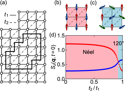
Figure 1: (a) Schematic representation of the ATL Hubbard model, where the solid and dashed lines represent the hopping integrals $t_{1}$ and $t_{2}$, respectively. The area surrounded by the thick solid line indicates the 12-site cluster used in our Lanczos calculations. (b), (c) Schematic illustrations of (b) the Néel order and (c) $120^{\circ}$ order. (d) Spin correlation function $S_{z}({\bm{q}},t=0)$ calculated for the ground state with the Néel order [${\bm{q}}=(\pi,\pi)$, red line] and $120^{\circ}$ order [${\bm{q}}=(2\pi/3,2\pi/3)$, blue line], where we assume $U/t_{1}=20$.

The ATL Hubbard model is defined by the Hamiltonian [see Fig. 1(a)]

$$\hat{\mathcal{H}}=-t_{1}\sum_{\langle i,j\rangle,s}\hat{c}_{i,s}^{\dagger}\hat{c}_{j,s}-t_{2}\sum_{\langle\langle i,j\rangle\rangle,s}\hat{c}_{i,s}^{\dagger}\hat{c}_{j,s}+U\sum_{i}\hat{n}_{i,\uparrow}\hat{n}_{i,\downarrow},$$ (1)

where $\hat{c}^{\quantity(\dagger)}_{i,s}$ is the annihilation (creation) operator of an electron at site $i$ with spin $s$, and $\hat{n}_{i,s}=\hat{c}^{\dagger}_{i,s}\hat{c}_{i,s}$ is the electron density operator. $t_{1}$ and $t_{2}$ are the nearest-neighbor (NN) and next-nearest-neighbor (NNN) hopping integrals, respectively, and $U$ is the on-site Coulomb interaction. The notations $\langle i,j\rangle$ and $\langle\langle i,j\rangle\rangle$ represent the pairs of the NN and NNN sites, respectively. In the strong-coupling limit $U/t_{1}\rightarrow\infty$ at half filling, the Hubbard model in Eq. (1) is mapped onto the antiferromagnetic Heisenberg model defined by

$$\hat{\mathcal{H}}_{\text{eff}}=J_{1}\sum_{\langle i,j\rangle}\hat{\bm{S}}_{i}\cdot\hat{\bm{S}}_{j}+J_{2}\sum_{\langle\langle i,j\rangle\rangle}\hat{\bm{S}}_{i}\cdot\hat{\bm{S}}_{j},$$ (2)

where $\hat{\bm{S}}_{i}$ is the spin-1/2 operator at site $i$, and $J_{1}=4t_{1}^{2}/U$ and $J_{2}=4t_{2}^{2}/U$ are the NN and NNN exchange interactions, respectively. The ground state of this model is of Néel type [Fig. 1(b)] at $J_{2}/J_{1}<0.83$, which switches to $120^{\circ}$ type [Fig. 1(c)] at $J_{2}/J_{1}>0.83$ Weihong1999PRB ; Yunoki2006PRB .

The time-dependent external field is introduced via the Peierls phase. Then, the hopping integrals are modified as

$$t_{n}\hat{c}_{i,\sigma}^{\dagger}\hat{c}_{j,s}\rightarrow t_{n}e^{-i\bm{A}(t)\dotproduct(\bm{r}_{i}-\bm{r}_{j})}\hat{c}_{i,\sigma}^{\dagger}\hat{c}_{j,s},$$ (3)

where $\bm{A}(t)$ is the vector potential at time $t$. In the present study, we use the vector potential parallel to the NNN direction, i.e., $\bm{A}(t)=\frac{1}{\sqrt{2}}\quantity[A(t),A(t)]$, where

$$A(t)=\begin{cases}A_{0}e^{-(t-t_{0})^{2}/2\sigma_{\mathrm{p}}^{2}}\cos\quantity[\omega_{\mathrm{p}}\quantity(t-t_{0})]&(t\leq t_{0})\\ A_{0}\cos\quantity[\omega_{p}\quantity(t-t_{0})]&(t>t_{0})\end{cases}$$ (4)

with the amplitude $A_{0}$ and frequency $\omega_{\mathrm{p}}$. In the following, we assume $\sigma_{\mathrm{p}}=2.0/t_{1}$ and $t_{0}=10/t_{1}$. We set the Planck constant $\hbar$, speed of light $c$, elementary charge $e$, and lattice constant to be unity.

Since the Hamiltonian depends on time in the presence of an external field, we need to solve the Schrödinger equation to obtain the time evolution of the wave function. We employ the time-dependent Lanczos method Park1986JCP ; Mohankumar2006CPC for this purpose. The time evolution with a time step $\delta t$ is calculated in the corresponding Krylov subspace generated by $M_{\mathrm{L}}$ Lanczos iterations. We use the 12-site cluster illustrated in Fig. 1(a) with periodic boundary conditions, and adopt $\delta t=0.01/t_{1}$ and $M_{\mathrm{L}}=15$. As the initial state, we assume $\ket{\psi(t=0)}=\ket{\psi_{0}}$, where $\ket{\psi_{0}}$ is the ground state of the Hamiltonian without an external field.

To determine the type of magnetic orders, we calculate the spin correlation function with momentum $\bm{q}$ at time $t$ written as

$$S_{z}(\bm{q},t)=\frac{1}{L}\sum_{i,j}S^{z}_{ij}(t)e^{i\bm{q}\dotproduct\quantity(\bm{r}_{i}-\bm{r}_{j})},$$ (5)

where $S^{z}_{ij}(t)=\matrixelement{\psi(t)}{\hat{S}^{z}_{i}\hat{S}^{z}_{j}}{\psi(t)}$ is the spin correlation in the real space. The ordering vector $\bm{q}=\bm{Q}_{\text{N\'{e}el}}=(\pi,\pi)$ and $\bm{q}=\bm{Q}_{120^{\circ}}=(2\pi/3,2\pi/3)$ correspond to the Néel order and $120^{\circ}$ order, respectively. The spin correlation functions calculated as a function of $t_{2}/t_{1}$ at $U/t_{1}=20$ are illustrated in Fig. 1(d), where we clearly find the phase transition from the Néel order to the $120^{\circ}$ order at $t_{2}/t_{1}\simeq 0.93$. Throughout the main text of this Letter, we use the values $U/t_{1}=20$ and $t_{2}/t_{1}=0.95$, for which the ground state is the $120^{\circ}$ order. Other cases, where the ground state has the the Néel order and the nearest-neighbor hopping integral satisfies $t_{2}/t_{1}=1$, are also discussed in Supplemental Material SM . We also define the time average of the spin correlation function from time $t=t_{\mathrm{i}}$ to $t_{\mathrm{f}}$ as

$$\bar{S}_{z}(\bm{q})=\frac{1}{t_{\mathrm{f}}-t_{\mathrm{i}}}\int^{t_{\mathrm{f}}}_{t_{\mathrm{i}}}\differential{t}S_{z}(\bm{q},t)$$ (6)

and the difference between the time average and initial value as $\Delta S_{z}(\bm{q})=\bar{S}_{z}(\bm{q})-S_{z}(\bm{q},t=0)$.

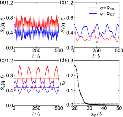
Figure 2: Calculated time evolution of the spin correlation function $S_{z}(\bm{q},t)$ at $\bm{q}=(\pi,\pi)$ (red line) and at $\bm{q}=(2\pi/3,2\pi/3)$ (blue line), where we assume $\omega_{\mathrm{p}}/t_{1}=30$ with (a) $A_{0}=1.0$, (b) $A_{0}=2.0$, and (c) $A_{0}=4.0$. Here, the dashed lines indicate $\bar{S}_{z}(\bm{q})$ averaged from $t_{\mathrm{i}}=10/t_{1}$ to $t_{\mathrm{f}}=500/t_{1}$. In (d), we show the calculated double occupancy $\bar{n}_{\mathrm{d}}$ averaged from $t_{\mathrm{i}}=10/t_{1}$ to $t_{\mathrm{f}}=500/t_{1}$, assuming $A_{0}=4.0$. The dashed line indicates the value of $n_{\mathrm{d}}(t=0)$.

The calculated results for the spin correlation function $S_{z}(\bm{q},t)$ as a function of time are shown in Figs. 2(a)-2(c). We find that, with the irradiation of light with $A_{0}=1.0$ and $\omega_{\mathrm{p}}=30/t_{1}$, the $120^{\circ}$ order stable in the ground state is switched to the Néel order [see Fig. 2(a)], which clearly indicates a magnetic phase transition induced by an external field. However, when we increase the amplitude of the external field to $A_{0}=2.0$, the state remains to be of $120^{\circ}$ order after the light irradiation [see Fig. 2(a)]. When we continue to increase the amplitude to $A_{0}=4.0$, the system again shows a transition to the Néel order [see Fig. 2(c)]. The present results suggest that the light-induced phase transition may occur in the ATL Hubbard model by adjusting the intensity of light. We note that the possibility of transitions to other types of orders is excluded from the analysis of the real-space spin correlation functions, as discussed in the Supplemental Material SM .

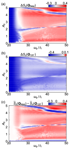
Figure 3: Differences in the spin correlation function calculated in the parameter space $(\omega_{\mathrm{p}}/t_{1},A_{0})$. Shown are (a) $\Delta S_{z}(\bm{Q}_{\text{N\'{e}el}})$, (b) $\Delta S_{z}(\bm{Q}_{120^{\circ}})$, and (c) $\bar{S}_{z}(\bm{Q}_{\text{N\'{e}el}})-\bar{S}_{z}(\bm{Q}_{120^{\circ}})$.

To explore the parameter regions where the $120^{\circ}$ order remains or the Néel order overcomes after the light irradiation, we calculate the difference in the spin correlation function $\Delta S_{z}(\bm{q})$ in the parameter space $(\omega_{\mathrm{p}}/t_{1},A_{0})$. The results are shown in Fig. 3(a) for the Néel order and in Fig. 3(b) for the $120^{\circ}$ order. These results clearly indicate that when the $120^{\circ}$ order is suppressed, the Néel order is complementarily enhanced. In addition, both orders are strongly suppressed at $\omega_{\mathrm{p}}/t_{1}<25$, where we note that the double occupancy defined as

$$n_{\mathrm{d}}(t)=\frac{1}{L}\sum_{i}\bra{\psi(t)}\hat{n}_{i,\uparrow}\hat{n}_{i,\downarrow}\ket{\psi(t)}$$ (7)

increases [see Fig. 2(d)] and therefore the charge excitations occurring across the Mott-Hubbard gap ($\simeq U/t_{1}$) increase, leading to the suppression of spin fluctuations. In Fig. 3(c), we show the calculated result for $\bar{S}_{z}(\bm{Q}_{\text{N\'{e}el}})-\bar{S}_{z}(\bm{Q}_{120^{\circ}})$. This result indicates which order is realized in the parameter space after the light irradiation; in the red region, the Néel order appears, while in the blue region, the $120^{\circ}$ order remains.

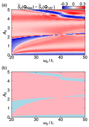
Figure 4: (a) Difference $\bar{S}_{z}(\bm{Q}_{\text{N\'{e}el}})-\bar{S}_{z}(\bm{Q}_{120^{\circ}})$ calculated for the effective Heisenberg model Eq. (8) in the parameter space $(\omega_{\mathrm{p}}/t_{1},A_{0})$. (b) Ratio of the Floquet effective exchange interactions, where the region of $J_{2}^{\text{eff}}/J_{1}^{\text{eff}}<0.83$ ($J_{2}^{\text{eff}}/J_{1}^{\text{eff}}>0.83$) is indicated by the red (blue) color.

To discuss the origin of the light-induced phase transition, we analyze the model using the Floquet theory Mentink2015NC ; Kitamura2016PRB . Applying the high-frequency expansion to our Hubbard-model Hamiltonian with an external field $A(t)=A_{0}\cos\omega_{\mathrm{p}}t$, we obtain the effective Hamiltonian in the strong-coupling limit as Kitamura2016PRB

$$\hat{\mathcal{H}_{\text{eff}}}=J_{1}^{\text{eff}}\sum_{\langle i,j\rangle}\hat{\bm{S}}_{i}\cdot\hat{\bm{S}}_{j}+J_{2}^{\text{eff}}\sum_{\langle\langle i,j\rangle\rangle}\hat{\bm{S}}_{i}\cdot\hat{\bm{S}}_{j},$$ (8)

where

$$J_{1}^{\text{eff}} =\sum_{m=-\infty}^{\infty}(-1)^{m}\frac{4t_{1}^{2}\mathcal{J}_{m}(A_{0}/\sqrt{2})}{U+m\omega_{\mathrm{p}}}$$ (9)

and

$$J_{2}^{\text{eff}} =\sum_{m=-\infty}^{\infty}(-1)^{m}\frac{4t_{2}^{2}\mathcal{J}_{m}(\sqrt{2}A_{0})}{U+m\omega_{\mathrm{p}}}$$ (10)

are the NN and NNN Floquet effective exchange interactions, respectively. Here, $\mathcal{J}_{m}(x)$ is the $m$-th Bessel function. Using this model, we perform the calculation of the quench dynamics Kawamura2017CPC , where $J_{1}$ and $J_{2}$ are suddenly changed to $J_{1}^{\text{eff}}$ and $J_{2}^{\text{eff}}$, respectively, at $t=0$. The result for the difference $\bar{S}_{z}(\bm{Q}_{\text{N\'{e}el}})-\bar{S}_{z}(\bm{Q}_{120^{\circ}})$ thus calculated is shown in Fig. 4(a) in the parameter space $(\omega_{\mathrm{p}}/t_{1},A_{0})$, which we find is consistent with the result obtained for the Hubbard model at least in the region $\omega_{\mathrm{p}}/t_{1}\gtrsim 25$ [see Fig. 3(c)]. The inconsistency found in the region $\omega_{\mathrm{p}}/t_{1}\lesssim 25$ comes from the enhancement of the double occupancy, which cannot be explained by the strong-coupling expansion. We thus conclude that in a regime of sufficiently high frequency, the result obtained from the Floquet effective Hamiltonian Eq. (8) well explains the behaviors of the Hubbard model in the strong-coupling region under a time-periodic external field.

We also calculate the phase diagram of the effective Hamiltonian simply from the ratio of the effective exchange interactions $J_{2}^{\text{eff}}/J_{1}^{\text{eff}}$. The result is shown in Fig. 4(b), where the phase boundary is determined as the line $J_{2}/J_{1}=0.83$, at which the phase transition between the Néel and $120^{\circ}$ orders occurs in the ground state of the ATL Heisenberg model. We thus find that the Néel order is preferred in the red region ($J_{2}^{\text{eff}}/J_{1}^{\text{eff}}<0.83$), while the $120^{\circ}$ order is preferred in the blue region ($J_{2}^{\text{eff}}/J_{1}^{\text{eff}}>0.83$). We thus clearly find that the phase diagram obtained by the quench-dynamics calculation is consistent with the phase diagram determined from the ratio of the exchange interactions, implying that the magnetic order realized by the light irradiation can be predicted from the Floquet theory.

We note that there are regions where $J^{\mathrm{eff}}_{1}<0$ and $J^{\mathrm{eff}}_{2}<0$, i.e., the regions where the ground state of the Hamiltonian Eq. (8) is ferromagnetic. Our calculated results, however, do not indicate the presence of such regions. This is because the electric field never flips the spins, or the total spin is conserved by light irradiation. In addition, since the time evolution of the sign-reversed Hamiltonian is exactly identical with the reversed time evolution of the original Hamiltonian Mentink2015NC , we can discuss the dynamics of an effective Hamiltonian with $J^{\mathrm{eff}}_{1}<0$ and $J^{\mathrm{eff}}_{2}<0$ by using the effective Hamiltonian with $J^{\mathrm{eff}}_{1}>0$ and $J^{\mathrm{eff}}_{2}>0$. We also note that there is a region where $J_{1}^{\text{eff}}\cdot J_{2}^{\text{eff}}<0$. It is known that the Néel order is preferred in the case of $J_{1}^{\text{eff}}>0$ and $J_{2}^{\text{eff}}<0$ Schmidt2014PRB , and thus the whole phase diagram can again be interpreted from the Floquet theory.

In summary, we have investigated the time dependence of the spin correlations of an anisotropic triangular Hubbard model at half filling under a time-periodic external electric field using the time-dependent Lanczos method. We have shown that the $120^{\circ}$ order can be switched to the Néel order by tuning the frequency and amplitude of the external field. To understand the magnetic phase transition under a periodic field, we have introduced the effective Heisenberg-model Hamiltonian by high-frequency expansion. The phase diagram obtained from the quench dynamics of this effective model is consistent with the results of our Hubbard-model calculations, which implies that the phase diagram obtained by light irradiation can be interpreted by the Floquet theory. Thus, the switching of magnetic orders can be realized in a frustrated spin system by tuning the amplitude and frequency of the external field. We hope that our results will shed some light on the possible realization of the photo-control of magnetic orders in frustrated spin systems.

This work was supported in part by Grants-in-Aid for Scientific Research from JSPS (Projects No. JP17K05530, No. JP19J20768, No. JP19K14644, and No. JP20H01849). R.F. acknowledges support from the JSPS Research Fellowship for Young Scientists. We acknowledge the use of open-source software $\mathcal{H}\Phi$ Kawamura2017CPC .

References

- (1) D. Fausti, R. I. Tobey, N. Dean, S. Kaiser, A. Dienst, M. C. Hoffmann, S. Pyon, T. Takayama, H. Takagi, and A. Cavalleri, Science 331, 189 (2011).
- (2) W. Hu, S. Kaiser, D. Nicoletti, C. R. Hunt, I. Gierz, M. C. Hoffmann, M. Le Tacon, T. Loew, B. Keimer, and A. Cavalleri, Nat. Mater. 13, 705 (2014).
- (3) M. Mitrano, A. Cantaluppi, D. Nicoletti, S. Kaiser, A. Perucchi, S. Lupi, P. Di Pietro, D. Pontiroli, M. Riccò, S. R. Clark, D. Jaksch, and A. Cavalleri, Nature (London) 530, 461 (2016).
- (4) T. Suzuki, T. Someya, T. Hashimoto, S. Michimae, M. Watanabe, M. Fujisawa, T. Kanai, N. Ishii, J. Itatani, S. Kasahara, Y. Matsuda, T. Shibauchi, K. Okazaki, and S. Shin, Commun. Phys. 2, 115 (2019).
- (5) M. Buzzi, D. Nicoletti, M. Fechner, N. Tancogne-Dejean, M. A. Sentef, A. Georges, T. Biesner, E. Uykur, M. Dressel, A. Henderson, T. Siegrist, J. A. Schlueter, K. Miyagawa, K. Kanoda, M.-S. Nam, A. Ardavan, J. Coulthard, J. Tindall, F. Schlawin, D. Jaksch, and A. Cavalleri, Phys. Rev. X 10, 031028 (2020).
- (6) A. Kogar, A. Zong, P. E. Dolgirev, X. Shen, J. Straquadine, Y. Q. Bie, X. Wang, T. Rohwer, I. C. Tung, Y. Yang, R. Li, J. Yang, S. Weathersby, S. Park, M. E. Kozina, E. J. Sie, H. Wen, P. Jarillo-Herrero, I. R. Fisher, X. Wang, and N. Gedik, Nat. Phys. 16, 159 (2020).
- (7) S. Mor, M. Herzog, D. Golež, P. Werner, M. Eckstein, N. Katayama, M. Nohara, H. Takagi, T. Mizokawa, C. Monney, and J. Stähler, Phys. Rev. Lett. 119, 086401 (2017).
- (8) K. Okazaki, Y. Ogawa, T. Suzuki, T. Yamamoto, T. Someya, S. Michimae, M. Watanabe, Y. Lu, M. Nohara, H. Takagi, N. Katayama, H. Sawa, M. Fujisawa, T. Kanai, N. Ishii, J. Itatani, T. Mizokawa, and S. Shin, Nat. Commun. 9, 4322 (2018).
- (9) M. Sato, S. Takayoshi, and T. Oka, Phys. Rev. Lett. 117, 147202 (2016).
- (10) T. Oka and S. Kitamura, Annu. Rev. Condens. Matter Phys. 10, 387 (2019).
- (11) J. H. Mentink, K. Balzer, and M. Eckstein, Nat. Commun. 6, 6708 (2015).
- (12) S. Kitamura and H. Aoki, Phys. Rev. B 94, 174503 (2016).
- (13) N. Dasari and M. Eckstein, Phys. Rev. B 100, 121114(R) (2019).
- (14) M. A. Sentef, A. Tokuno, A. Georges, and C. Kollath, Phys. Rev. Lett. 118, 087002 (2017).
- (15) R. Fujiuchi, T. Kaneko, K. Sugimoto, S. Yunoki, and Y. Ohta, Phys. Rev. B 101, 235122 (2020).
- (16) A. Eckardt, Rev. Mod. Phys. 89, 011004 (2017).
- (17) R. V. Mikhaylovskiy, E. Hendry, A. Secchi, J. H. Mentink, M. Eckstein, A. Wu, R. V. Pisarev, V. V. Kruglyak, M. I. Katsnelson, T. Rasing, and A. V. Kimel, Nat. Commun. 6, 8190 (2015).
- (18) E. A. Stepanov, C. Dutreix, and M. I. Katsnelson, Phys. Rev. Lett. 118, 157201 (2017).
- (19) S. Kitamura, T. Oka, and H. Aoki, Phys. Rev. B 96, 014406 (2017).
- (20) M. Claassen, H.-C. Jiang, B. Moritz, and T. P. Devereaux, Nat. Commun. 8, 1192 (2017).
- (21) K. Takasan and M. Sato, Phys. Rev. B 100, 060408(R) (2019).
- (22) S. Jana, P. Mohan, A. Saha, and A. Mukherjee, Phys. Rev. B 101, 115428 (2020).
- (23) N. Bittner, D. Golež, M. Eckstein, and P. Werner, Phys. Rev. B 102, 235169 (2020).
- (24) T. Mizusaki and M. Imada, Phys. Rev. B 74, 014421 (2006).
- (25) Z.-Q. Yu and L. Yin, Phys. Rev. B 81, 195122 (2010).
- (26) A. Yamada, Phys. Rev. B 89, 195108 (2014).
- (27) M. Laubach, R. Thomale, C. Platt, W. Hanke, and G. Li, Phys. Rev. B 91, 245125 (2015).
- (28) K. Misumi, T. Kaneko, and Y. Ohta, J. Phys. Soc. Jpn. 85, 064711 (2016).
- (29) R. Coldea, D. A. Tennant, K. Habicht, P. Smeibidl, C. Wolters, and Z. Tylczynski, Phys. Rev. Lett. 88, 137203 (2002).
- (30) T. Ono, H. Tanaka, H. Aruga Katori, F. Ishikawa, H. Mitamura and T.Goto, Phys. Rev. B 67, 104431 (2003).
- (31) S. Lefebvre, P. Wzietek, S. Brown, C. Bourbonnais, D. Jérome, C. Mézière, M. Fourmigué, and P. Batail, Phys. Rev. Lett. 85, 5420 (2000).
- (32) Y. Shimizu, K. Miyagawa, K. Kanoda, M. Maesato, and G. Saito,Phys. Rev. Lett.91, 107001 (2003).
- (33) Zheng Weihong, R. H. McKenzie, and R. R. P. Singh, Phys. Rev. B 59, 14367 (1999).
- (34) S. Yunoki and S. Sorella, Phys. Rev. B 74, 014408 (2006).
- (35) T. J. Park and J. Light, J. Chem. Phys. 85, 5870 (1986).
- (36) N. Mohankumar and S. M. Auerbach, Comput. Phys. Commun. 175, 473 (2006).
- (37) See Supplemental Material for details, which includes Refs. Hotta2012Crystals ; Dean2016NM ; Adachi1980JPSJ ; Shirata2012PRL ; Zhou2012PRL ; Ma2016PRL ; Ito2017NC ; Haraguchi2015PRB ; Iida2019SR ; Eckardt2010EPL ; Struck2011Science ; Messer2018PRL ; Sandholzer2019PRL .
- (38) C. Hotta, Crystals 2, 1155 (2012).
- (39) M. P. M. Dean, Y. Cao, X. Liu, S. Wall, D. Zhu, R. Mankowsky, V. Thampy, X. M. Chen, J. G. Vale, D. Casa, J. Kim, A. H. Said, P. Juhas, R. Alonso-Mori, J. M. Glownia, A. Robert, J. Robinson, M. Sikorski, S. Song, M. Kozina et al., Nat. Mater. 15, 601 (2016).
- (40) K. Adachi, N. Achiwa, and M. Mekata, J. Phys. Soc. Jpn. 49, 545 (1980).
- (41) Y. Shirata, H. Tanaka, A. Matsuo, and K. Kindo, Phys. Rev. Lett. 108, 057205 (2012).
- (42) H. D. Zhou, C. Xu, A. M. Hallas, H. J. Silverstein, C. R. Wiebe, I. Umegaki, J. Q. Yan, T. P. Murphy, J.-H. Park, Y. Qiu, J. R. D. Copley, J. S. Gardner, and Y. Takano, Phys. Rev. Lett. 109, 267206 (2012).
- (43) J. Ma, Y. Kamiya, T. Hong, H. B. Cao, G. Ehlers, W. Tian, C. D. Batista, Z. L. Dun, H. D. Zhou, and M. Matsuda, Phys. Rev. Lett. 116, 087201 (2016).
- (44) S. Ito, N. Kurita, H. Tanaka, S. Ohira-Kawamura, K. Nakajima, S. Itoh, K. Kuwahara, and K. Kakurai, Nat. Commun. 8, 235 (2017).
- (45) Y. Haraguchi, C. Michioka, M. Imai, H. Ueda, and K. Yoshimura, Phys. Rev. B 92, 014409 (2015).
- (46) K. Iida, H. Yoshida, H. Okabe, N. Katayama, Y. Ishii, A. Koda, Y. Inamura, N. Murai, M. Ishikado, R. Kadono, and R. Kajimoto, Sci. Rep. 9, 1826 (2019).
- (47) A. Eckardt, P. Hauke, P. Soltan-Panahi, C. Becker, K. Sengstock, and M. Lewenstein, EPL 89, 10010 (2010).
- (48) J. Struck, C. Olschlager, R. Le Targat, P. Soltan-Panahi, A. Eckardt, M. Lewenstein, P. Windpassinger, and K. Sengstock, Science 333, 996 (2011).
- (49) M. Messer, K. Sandholzer, F. Görg, J. Minguzzi, R. Desbuquois, and T. Esslinger, Phys. Rev. Lett. 121, 233603 (2018).
- (50) K. Sandholzer, Y. Murakami, F. Görg, J. Minguzzi, M. Messer, R. Desbuquois, M. Eckstein, P. Werner, and T. Esslinger, Phys. Rev. Lett. 123, 193602 (2019).
- (51) M. Kawamura, K. Yoshimi, T. Misawa, Y. Yamaji, S. Todo, and N. Kawashima, Comput. Phys. Commun. 217, 180 (2017).
- (52) B. Schmidt and P. Thalmeier, Phys. Rev. B 89, 184402 (2014).