Spin observables of proton-deuteron elastic scattering at SPD NICA energies within the Glauber model and pN amplitudes

Abstract

A systematic analysis of nucleon-nucleon scattering amplitudes is available up to a laboratory energy of $3$ GeV in case of the $pp$ system and up to $1.2$ GeV for $pn$. At higher energies there is only incomplete experimental information on $pp$ elastic scattering, whereas data for the $pn$ system are very scarce. We apply the spin-dependent Glauber theory to calculate spin observables of $pd$ elastic scattering at $3$-$50$ GeV/c using $pp$ amplitudes available in the literature and parametrized within the Regge formalism. The calculated vector $A_{y}^{p}$, $A_{y}^{d}$ and tensor $A_{xx}$, $A_{yy}$ analyzing powers and the spin-correlation coefficients $C_{y,y}$, $C_{x,x}$, $C_{yy,y}$, $C_{xx,y}$ can be measured at SPD NICA and, thus, will provide a test of the used $pN$ amplitudes.

^a Joint Institute for Nuclear Researches, Dubna, Moscow reg. 141980 Russia ^b Dubna State University, Dubna, Moscow reg. 141980 Russia ^c  Department of Physics, M.V. Lomonosov State University, Moscow, 119991 Russia ^d Institute for Advanced Simulation and Institut für Kernphysik, Forschungszentrum Jülich GmbH, D-52425 Jülich, Germany ^e L.N. Gumilyov Eurasian National University, Nur-Sultan, 010000, Kazakhstan ^f Institute of Nuclear Physics, Astana branch, Nur-Sultan, 010000, Kazakhstan

PACS: 44.25.$+$f; 44.90.$+$c

Introduction

The spin amplitudes of $pp$ and $pn$ elastic scattering contain important information on the dynamics of the $NN$ interaction. A systematic reconstruction of these amplitudes from scattering data is provided by the SAID partial-wave analysis [1] and covers laboratory energies up to $3$ GeV ($p_{lab}\approx 3.8$ GeV/c) for $pp$ and $1.2$ GeV ($p_{lab}\approx 1.9$ GeV/c) for $pn$ scattering. At higher energies there is only incomplete experimental information on $pp$ scattering, whereas data for the $pn$ system are very scarse. In the literature there are some parametrizations for $pN$ amplitudes, obtained in the eikonal model [2] for the laboratory momentum $6$ GeV/c and within the Regge phenomenology [3] for $3$-$50$ GeV/c (corresponding to $2.77<\sqrt{s}<10$ GeV). Another Regge-type parametrization for values of $s$ above $6$ GeV² ($p_{lab}\geq 2.2$ GeV/c) was presented in Ref. [4]. A possible way to check existing parametrizations is to study spin effects in proton-deuteron ($pd$) and neutron-deuteron ($nd$) elastic and quasi-elastic scattering. At high energies and small four-momentum transfer $t$, $pd$ scattering can be described by the Glauber diffraction theory of multistep scattering, which involves as input on-shell $pN$ elastic scattering amplitudes. Applications of this theory with spin-dependent effects included [5] indicate a good agreement with the $pd$ scattering data at energies about $1$ GeV if the SAID values for the $pN$ scattering amplitudes are used as starting point of the calculations [6, 7, 8].

In the present work we apply the spin-dependent Glauber theory [5, 6] to calculate spin observables of $pd$ elastic scattering at $5$-$50$ GeV/c utilizing the $pp$ elastic scattering amplitudes established and parametrized in Ref. [3] within the Regge formalism. As a first approximation, for the $pn$ amplitudes we use likewise the ones for $pp$ from [3]. We should note that, in principle, the Regge approach allows one to construct $pn$ (and $\bar{p}N$) amplitudes together with the $pp$ amplitudes. However, in view of the scarce experimental information on the spin-dependent $pn$ amplitudes and taking into account that the spin-independent parts of the $pp$ and $pn$ amplitudes at high energies are approximately the same, we assume here that the whole $pn$ amplitude is the same as that for $pp$. The calculated vector $A_{y}^{p}$, $A_{y}^{d}$ and tensor analyzing powers $A_{xx}$, $A_{yy}$, and the spin-correlation coefficients $C_{y,y}$, $C_{x,x}$, $C_{yy,y}$, $C_{xx,y}$ can be measured at SPD NICA [9], which will provide a serious test of the used $pN$ amplitudes. A knowledge of $pN$ helicity amplitudes is required in preparation and subsequent analysis of experiments for search of time-reversal invariance violation effects in double-polarized $pd$ scattering [10, 11].

Elements of formalism

The reaction amplitude $pd\to pd$ can be written as [6]

$$<p^{\prime}\mu^{\prime},d^{\prime}\lambda^{\prime}|T|p\mu,d\lambda>=\varphi^{+}_{\mu^{\prime}}{e_{\beta}^{(\lambda^{\prime})}}^{*}T_{\beta\alpha}({\bf p},{\bf p}^{\prime},{\mbox{\boldmath$\sigma$}})e_{\alpha}^{(\lambda)}\varphi_{\mu},$$ (1)

where $\varphi_{\mu}$ ($\varphi_{\mu^{\prime}}$) is the Pauli spinor of the initial (final) proton in the state with spin projecion $\mu$ ($\mu^{\prime}$) onto the quantization axis, $e_{\alpha}^{(\lambda)}$ ($e_{\beta}^{(\lambda^{\prime})}$) is the polarization vector of the initial $d$ (final $d^{\prime}$) deuteron in the state with the spin projection $\lambda$ ($\lambda^{\prime}$), and $T_{\beta\alpha}$ is the dynamical tensor ($\beta,\alpha$=$x,y,z$) acting in the spin space of the proton. The latter depends on the momentum of the initial ($\bf p$) and final (${\bf p}^{\prime}$) proton and contains the Pauli spin matrices ${{\mbox{\boldmath$\sigma$}}}=(\sigma_{x},\ \sigma_{y},\ \sigma_{z})$. We use the Madison reference frame with the axis OZ$||$${\bf p}$, OY$||$$[{\bf p}\times{\bf p}^{\prime}]$ and OX choosen in such a way to provide a right-handed coordinate system. Using the method of Ref. [12] for the transition tensor $T_{\beta\alpha}$ and assuming parity (P) conservation, one has, in the general case, independently of the dynamics of the considered process,

$$\begin{array}[]{ccc}T_{xx}=M_{1}+M_{2}\sigma_{y}&T_{xy}=M_{7}\sigma_{z}+M_{8}\sigma_{x}&T_{xz}=M_{9}+M_{10}\sigma_{y}\\ T_{yx}=M_{13}\sigma_{z}+M_{14}\sigma_{x}&T_{yy}=M_{3}+M_{4}\sigma_{y}&T_{yz}=M_{11}\sigma_{x}+M_{12}\sigma_{z}\\ T_{zx}=M_{15}+M_{16}\sigma_{y}&T_{zy}=M_{17}\sigma_{x}+M_{18}\sigma_{z}&T_{zz}=M_{5}+M_{6}\sigma_{y},\end{array}$$ (5)

where $M_{i}$ ($i=1,\dots,18$) are complex amplitudes determined by the dynamics of the reaction. As was mentioned in Ref. [6], under the operation of time reversal this reference frame is rotated around the OY axis on the scattering angle $\theta$ that is the angle between the vectors $\bf p$ and $\bf p^{\prime}$. This complicates the formulation of the time-reversal (T) invariance conditions as compared to other (non-Madison) reference frames, like in Ref. [5] and, therefore, we do not write them explicitly. However, the amplitudes $M_{i}$ ($i=1,\dots,18$) satisfy T-reversal invariance since they are explicitly expressed as linear combinations of the T-reversal invariant amplitudes $A_{i}$ ($i=1,\dots,12$) of $pd$ scattering introduced in Ref. [5].

The spin observables $A_{y}$, $A_{ij}$, and $C_{ij,k}$ defined in the notation of Ref. [13] and considered in the present work, have the following form in terms of the amplitudes $M_{i}$

$$\frac{d\sigma}{dt} = \frac{1}{6}TrMM^{+},\ \ \ \ \ \ TrMM^{+}=2\sum_{i=1}^{18}|M_{i}|^{2},$$ (6)

$$A_{y}^{d} = TrMS_{y}M^{+}/TrMM^{+}=$$

$$- \frac{2}{\sum_{i=1}^{18}|M_{i}|^{2}}Im(M_{1}M_{9}^{*}+M_{2}M_{10}^{*}+M_{13}M_{12}^{*}+M_{14}M_{11}^{*}+M_{15}M_{5}^{*}+M_{16}M_{6}^{*}),$$

$$A_{y}^{p} = TrM\sigma_{y}M^{+}/TrMM^{+}=$$

$$\frac{2}{\sum_{i=1}^{18}|M_{i}|^{2}}\Bigl{[}Re(M_{1}M_{2}^{*}+M_{9}M_{10}^{*}+M_{3}M_{4}^{*}+M_{15}M_{16}^{*}+M_{5}M_{6}^{*})-$$

$$Im(M_{8}M_{7}^{*}+M_{14}M_{13}^{*}+M_{11}M_{12}^{*}+M_{17}M_{18}^{*})\Bigr{]},$$

$$A_{yy} = TrM{\cal P}_{yy}M^{+}/TrMM^{+}=$$

$$1-\frac{3}{\sum_{i=1}^{18}}(|M_{3}|^{2}+|M_{4}|^{2}+|M_{7}|^{2}+|M_{8}|^{2}+M_{17}|^{2}+|M_{18}|^{2}),$$

$$A_{xx} = TrM{\cal P}_{yy}M^{+}/TrMM^{+}=$$

$$1-\frac{3}{\sum_{i=1}^{18}}(|M_{1}|^{2}+|M_{2}|^{2}+|M_{13}|^{2}+|M_{14}|^{2}+|M_{15}|^{2}+|M_{16}|^{2}),$$

$$C_{y,y} = TrM{S}_{y}\sigma_{y}M^{+}/TrMM^{+}=$$

$$-\frac{2}{\sum_{i=1}^{18}|M_{i}|^{2}}\Bigl{[}Im(M_{2}M_{9}^{*}+M_{1}M_{10}^{*}+M_{16}M_{5}^{*}+M_{15}M_{6}^{*})+$$

$$Re(M_{14}M_{12}^{*}-M_{13}M_{11}^{*})\Bigr{]},$$

$$C_{x,x} = TrM{S}_{y}\sigma_{y}M^{+}/TrMM^{+}=$$

$$-\frac{2}{\sum_{i=1}^{18}|M_{i}|^{2}}\bigl{[}Im(M_{8}M_{9}^{*}+M_{3}M_{11}^{*}+M_{17}M_{5}^{*})+$$

$$Re(M_{7}M_{10}^{*}-M_{4}M_{12}^{*}+M_{18}M_{6}^{*})\Bigr{]},$$

$$C_{xx,y} = TrM{}_{xx}\sigma_{y}M^{+}/TrMM^{+}=$$

$$=A_{y}^{p}-\frac{6}{\sum_{i=1}^{18}|M_{i}|^{2}}\frac{2}{\sum_{i=1}^{18}|M_{i}|^{2}}\bigl{[}Re(M_{2}M_{1}^{*}+M_{16}M_{15}^{*})-Im(M_{14}M_{13}^{*})$$

$$C_{yy,y} = TrM{}_{yy}\sigma_{y}M^{+}/TrMM^{+}=$$

$$- =A_{y}^{p}-\frac{6}{\sum_{i=1}^{18}|M_{i}|^{2}}\bigl{[}ReM_{3}M_{4}^{*}-Im(M_{17}M_{18}^{*}+M_{8}M_{7}^{*})\Bigr{]},$$

where ${\cal P}_{ij}=\frac{3}{2}(S_{i}S_{j}+S_{j}S_{i})-2\delta_{ij}$ and $S_{j}$ ($j=x,y,z$) are Cartesian components of the spin operator for the system with $S=1$.

In Ref. [5] (PK) the general spin structure of the transition operator $pd\to pd$ is written in a different representation and in another reference frame with axis $OX^{\prime}\uparrow\uparrow{\bf q}$, $OZ^{\prime}\uparrow\uparrow{\bf k}$, $OY^{\prime}\uparrow\uparrow{\bf n}$, where ${\hat{\bf q}}=({\bf p}-{\bf p}^{\prime})/|({\bf p}-{\bf p}^{\prime})|$, ${\hat{\bf k}}=({\bf p}+{\bf p}^{\prime})/|({\bf p}+{\bf p}^{\prime})|$, ${\hat{\bf n}}=[\bf{k}\times{\bf q}]$ forming the right-handed system (${\bf p}$ and ${\bf p}^{\prime}$ being the momenta of the incident and outgoing proton, respectively).

The amplitudes of $pN$ elastic scattering are written as [5]

$$M_{N}({\bf p},{\bf q};{\mbox{\boldmath$\sigma$}},{{\mbox{\boldmath$\sigma$}}}_{N})=A_{N}+C_{N}{\mbox{\boldmath$\sigma$}}\hat{n}+C_{N}^{\prime}{\mbox{\boldmath$\sigma$}}_{N}\hat{n}+B_{N}({\mbox{\boldmath$\sigma$}}\hat{\bf k})({\mbox{\boldmath$\sigma$}}_{N}\hat{\bf k})+$$ (7)

$$+(G_{N}+H_{N})({\mbox{\boldmath$\sigma$}}\hat{\bf q})({\mbox{\boldmath$\sigma$}}_{N}\hat{\bf q})+(G_{N}-H_{N})({\mbox{\boldmath$\sigma$}}\hat{\bf n})({\mbox{\boldmath$\sigma$}}_{N}\hat{\bf n}),$$

where the complex numbers $A_{N}$, $C_{N}$, $C_{N}^{\prime}$, $B_{N}$, $G_{N}$, $H_{N}$ were fixed from the amplitudes of the SAID analysis [1] and parametrized by a sum of Gaussians. For the double scattering term in $pd$ scattering the unit vectors $\hat{\bf k}$, $\hat{\bf q}$, $\hat{\bf n}$ are defined separately for each individual $NN$ collision.

The amplitude (7) is normalized in such a way that the invariant differential cross section has the following form:

$$\frac{d\sigma_{N}}{dt}=\frac{1}{4}TrM_{N}M_{N}^{+}.$$ (8)

Some additional results of calculations within this approach were reported recently in Ref. [8].

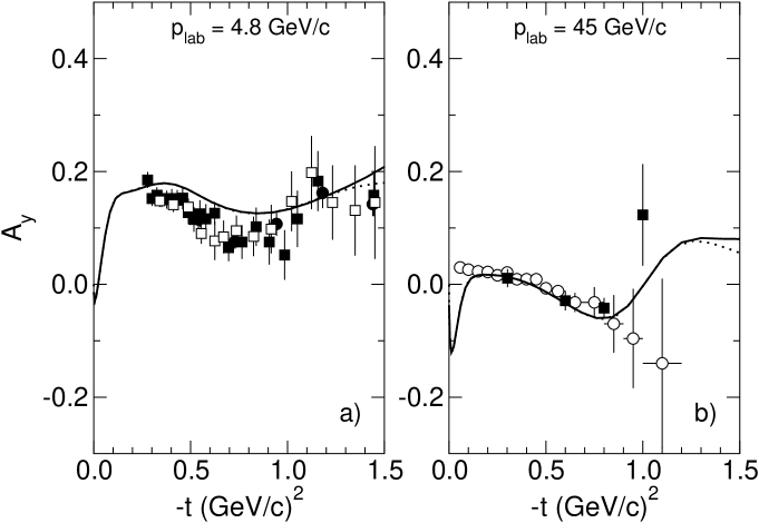
Figure 1: Analyzing power for $pp$ elastic scattering as a function of the four-momentum transfer $-t$ at $4.8$ GeV/c (left) and $45$ GeV/c (right). The dashed line is the result of the Regge model by Sibirtsev et al. [3] while the solid line is based on the parameterization in terms of exponential functions (Numerical results). Left: Data are taken from Refs. [14] (filled squares: $4.4$ GeV/c; open squares: $5.15$ GeV/c), and [15] (circles). Right: Data are taken from Refs. [16] (squares) and [17] (circles).

fig01

Numerical results

Table 1: Parameters of the $pN$ amplitudes at $p_{lab}=45$ GeV/c, cf. Eq. (Numerical results). The dimension $n$ for the coefficients $C_{\alpha,j}$ depends on the power of the $q$ factor in Eqs. (Numerical results) and is $n=1$ for $A_{p}$ and $G_{p}$, $n=2$ for $C_{p}$ and $n=3$ for $H_{p}$.

		real part		imaginary part
	j	$C_{\alpha,j}$ (mb1/2/GeVn)	$A_{\alpha,j}$ (GeV-2)	$C_{\alpha,j}$ (mb1/2/GeVn)	$A_{\alpha,j}$ (GeV-2)
	1	-0.10113182E+00	0.26000000E+01	-0.50868385E-01	0.26000000E+01
	2	-0.30272788E+00	0.39000000E+01	0.45135636E+01	0.45000000E+01
	3	0.36275621E-01	0.62769552E+01	0.54701498E+01	0.79740115E+01
$A_{p}$	4	0.69044456E+00	0.93549981E+01	-0.10151078E+02	0.12472690E+02
	5	-0.14278735E+01	0.13000000E+02	0.16289509E+02	0.17800000E+02
	6	0.12152644E+01	0.17134442E+02	-0.12268618E+02	0.23842646E+02
	7	-0.14350110E+01	0.21706020E+02	0.46423346E+01	0.30524183E+02
	1	0.74355080E-01	0.26000000E+01	0.45689189E-01	0.26000000E+01
	2	-0.16130899E+01	0.44000000E+01	-0.79107203E+00	0.38000000E+01
	3	0.45217973E+01	0.76911688E+01	0.57485752E+01	0.59941125E+01
$C_{p}$	4	-0.54780216E+01	0.11953074E+02	-0.85442702E+01	0.88353828E+01
	5	0.49658391E+01	0.17000000E+02	0.13994870E+02	0.12200000E+02
	6	0.49231089E+01	0.22724612E+02	-0.19190882E+02	0.16016408E+02
	7	0.10015797E+02	0.29054489E+02	0.18732648E+02	0.20236326E+02
	1	-0.74954883E+00	0.26000000E+01	-0.11871787E+01	0.26000000E+01
	2	0.40241315E+01	0.39000000E+01	0.53517954E+01	0.32000000E+01
	3	-0.12125361E+02	0.62769552E+01	-0.96756963E+01	0.42970562E+01
$G_{p}$	4	0.10072340E+02	0.93549981E+01	0.32522898E+01	0.57176913E+01
	5	-0.18247682E+01	0.13000000E+02	-0.89637709E+01	0.73999998E+01
	6	0.76091977E+00	0.17134442E+02	0.94782521E+01	0.93082036E+01
	7	-0.15772284E+00	0.21706020E+02	0.17443063E+01	0.11418163E+02
	1	0.31798006E+00	0.26000000E+01	0.43576664E+00	0.26000000E+01
	2	-0.33720909E+01	0.46000000E+01	-0.25451131E+01	0.34000000E+01
	3	0.24771736E+02	0.82568542E+01	0.42584276E+01	0.48627416E+01
$H_{p}$	4	-0.10758994E+02	0.12992305E+02	0.11014990E+02	0.67569218E+01
	5	0.15394572E+02	0.18600000E+02	0.19721651E+02	0.89999998E+01
	6	-0.13147804E+02	0.24960680E+02	-0.50146514E+00	0.11544272E+02
	7	0.45696137E+01	0.31993877E+02	0.48863565E+00	0.14357550E+02

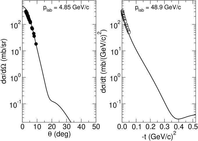
Figure 2: Differential cross section for $pd$ elastic scattering. Predictions are shown for $p_{lab}=4.8$ GeV/c (left) and $45$ GeV/c (right). Data are taken from Refs. [18] ($4.8$ GeV/c) and [19] ($48.9$ GeV/c).

fig02

The relations between the $pN$ amplitudes $A_{N}$, $B_{N}$, $C_{N}$, $G_{N}$, $H_{N}$ and the helicity amplitudes $\phi_{1},\,...,\,\phi_{5}$, and the corresponding expansion in terms of exponential functions are the following

$$A_{N}(q)=(\phi_{3}+\phi_{1})/2=\sum_{i}C_{a,j}\exp{(-A_{a,j}\,q^{2})},$$

$$B_{N}(q)=(\phi_{3}-\phi_{1})/2=\sum_{i}C_{b,j}\exp{(-A_{b,j}\,q^{2})},$$

$$C_{N}(q)=i\phi_{5}=q\sum_{i}C_{c,j}\exp{(-A_{c,j}\,q^{2})},$$

$$G_{N}(q)=\phi_{2}/2=\sum_{i}C_{g,j}\exp{(-A_{g,j}\,q^{2})},$$

$$H_{N}(q)=\phi_{4}/2=q^{2}\sum_{i}C_{h,j}\exp{(-A_{h,j}\,q^{2})},$$ (9)

where $q^{2}=-t$. Note that $C_{N}^{\prime}$ in Eq. (7) is given by $C_{N}^{\prime}(q)=C_{N}(q)+i\,(q/2m)\,A_{N}(q)$ [5], with $m$ being the nucleon mass.

Numerical values for the parameters of the Gaussians in Eqs. (Numerical results) are obtained by fitting to the helicity amplitudes from Ref. [3]. Those for $p_{lab}=45$ GeV/c are summary in Table 1. Note that the parameters for the real and imaginary parts of the amplitudes are given separately. Also, we would like to mention that $\phi_{1}\equiv\phi_{3}$ in the model by Sibirtsev et al., see Eq. (12) of that work, and, accordingly, $B_{N}\equiv 0$. The differential cross section of $pp$ elastic scattering and the vector anayzing power $A_{y}$ are reproduced with these parameterizations on the same level of accuracy as in Ref. [3], in the interval of transferred four momentum $-t<1.5$ (GeV/c)². As example, in Fig. LABEL:fig01 we show results for the latter, by the model (dotted line) and by the parameterization (solid line).

In the next step we performed calculations for the $pd$ observables listed in Eqs. (6) at $p_{lab}=4.68$ GeV/c and $45$ GeV/c, using these Gaussian parameterizations of the $pN$ amplitudes. Results for the differential cross section are shown in Fig. LABEL:fig02 while a selection of spin-dependent observables is presented in Figs. LABEL:fig03 and LABEL:fig04. In the latter figures the results at $4.68$ GeV/c are indicated by the dashed lines, those at $45$ GeV/c by solid lines. One can see from Fig. LABEL:fig02 that available data on the $pd$ elastic differential cross section in the forward hemisphere are well described by our calculations. As was mentioned in the Introduction, we assume here that the $pn$ amplitudes are identical to the $pp$ amplitudes. Fig. LABEL:fig03 shows that the vector analyzing power $A_{y}^{p}$ decreases significantly in absolute value with increasing energy and a similar behaviour is exhibited by $A_{y}^{d}$. In contrast, the spin correlation coefficients $C_{x,x}$ and $C_{y,y}$ show the opposite tendency, cf. Fig. LABEL:fig04. Coulomb effects are taken into account here in the $pp$ amplitude in the same way as in Ref. [6] and give a rather small contribution, as can be seen from Fig. LABEL:fig03a,b). One should note that the tensor analyzing powers $A_{xx}$ and $A_{yy}$, shown in Fig. LABEL:fig04, depend only weakly on the energy. Moreover, these observables do not change qualitatively in forward direction if all spin-dependent amplitudes are excluded and only the spin-independent amplitude $A_{N}$ from Eq. (7) is taken into account, cf. the dotted lines. On the hand, the spin correlation parameters $C_{x,x}$, $C_{y,y}$ practically vaninsh in this case (Fig. LABEL:fig04a,c)).

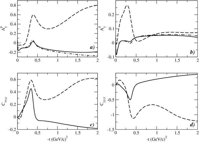
Figure 3: Results for spin-dependent $pd$ observables. Predictions for $p_{lab}=4.8$ Gev/c are shown by dashed lines while those at $45$ GeV/c correspond to the solid lines. The effect of the Coulomb interaction is indicated by the dash-dotted lines.

fig03

Conclusion

Nucleon-nucleon elastic scattering is a basic process in the physics of atomic nuclei and the interaction of hadrons with nuclei. Full information about the spin dependent $pN$ amplitudes can be obtained, in principle, from a complete polarization experiment, which, however, requires to measure twelve independent observables at a given collision energy and, thus, constitutes a too complicated experimental task. On the other hand existing models and corresponding parametrizations of $pp$ amplitudes in the region of small transferred momenta can be effectively tested by a measurement of spin observables for $pd$ scattering and a subsequent comparison of the results with corresponding Glauber calculations. The spin observables of $pd$ elastic scattering studied and evaluated in the

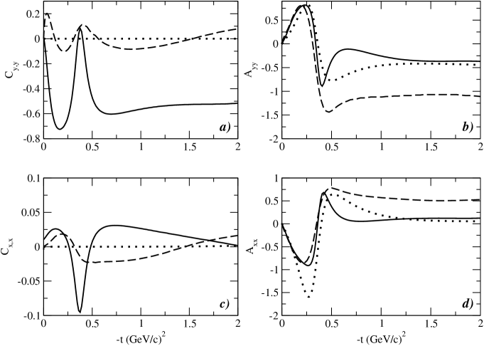
Figure 4: Results for spin-dependent $pd$ observables. Same description of curves as in Fig. LABEL:fig03. The dotted lines are results where the spin-dependent $pN$ amplitudes have been omitted in the calculation.

fig04

present work are found to be not too small and, thus, could be measured at the future SPD NICA facility.

Acknowledgements: A.B., A.T. and Yu.U. acknowledge their support by the Scientific Programme of JINR-Kazakhstan N 391-20.07.2020.

References

- [1] Arndt R., Briscoe W., Strakovsky I., Workman R. Updated analysis of NN elastic scattering to 3-GeV // Phys. Rev. C. — 2007. — V. 76. — P. 025209. — arXiv:0706.2195 [nucl-th].
- [2] Sawamoto M., Wakaizumi S. Analysis of elastic p p scattering at 6-GeV/c with spin orbit and spin spin coupling eikonals // Prog. Theor. Phys. — 1979. — V. 62. — P. 563–565.
- [3] Sibirtsev A., Haidenbauer J., Hammer H.W., Krewald S., Meißner U.G. Proton-proton scattering above 3 GeV/c // Eur. Phys. J. A. — 2010. — V. 45. — P. 357–372. — arXiv:0911.4637 [hep-ph].
- [4] Ford W.P., Van Orden J. Regge model for nucleon-nucleon spin-dependent amplitudes // Phys. Rev. C. — 2013. — V. 87, no. 1. — P. 014004. — arXiv:1210.2648 [nucl-th].
- [5] Platonova M., Kukulin V. Refined Glauber model versus Faddeev calculations and experimental data for spin observables // Phys. Rev. C. — 2010. — V. 81. — P. 014004. — [Erratum: Phys.Rev.C 94, 069902 (2016)] arXiv:1612.08694.
- [6] Temerbayev A., Uzikov Y. Spin observables in proton-deuteron scattering and T-invariance test // Phys. Atom. Nucl. — 2015. — V. 78, no. 1. — P. 35–42.
- [7] Mchedlishvili D., others. Deuteron analysing powers in deuteron–proton elastic scattering at 1.2 and 2.27 GeV // Nucl. Phys. A. — 2018. — V. 977. — P. 14–22. — arXiv:1805.05778.
- [8] Platonova M.N., Kukulin V.I. Theoretical study of spin observables in elastic scattering at energies = 800-1000 MeV // Eur. Phys. J. A. — 2020. — V. 56, no. 5. — P. 132. — arXiv:1910.05722.
- [9] Savin I., others. Spin Physics Experiments at NICA-SPD with polarized proton and deuteron beams // EPJ Web Conf. — 2015. — V. 85. — P. 02039. — arXiv:1408.3959 [hep-ex].
- [10] Uzikov Y.N., Temerbayev A. Null-test signal for -invariance violation in scattering // Phys. Rev. C. — 2015. — V. 92, no. 1. — P. 014002. — arXiv:1506.08303.
- [11] Uzikov Y.N., Haidenbauer J. Polarized proton-deuteron scattering as a test of time-reversal invariance // Phys. Rev. C. — 2016. — V. 94, no. 3. — P. 035501. — arXiv:1607.04409.
- [12] Uzikov Y. Backward elastic p d scattering at intermediate-energies // Phys. Part. Nucl. — 1998. — V. 29. — P. 583–605.
- [13] Ohlsen G.G. Polarization transfer and spin correlation experiments in nuclear physics // Rept. Prog. Phys. — 1972. — V. 35. — P. 717–801.
- [14] Parry J., Booth N., Conforto G., Esterling R., Scheid J., Sherden D., Yokosawa A. Measurements of the polarization in proton proton elastic scattering from 2.50 to 5.15 gev/c // Phys. Rev. D. — 1973. — V. 8. — P. 45–63.
- [15] Abshire G., Ankenbrandt C., Crittenden R., Heinz R., Hinotani K., Neal H., Rust D. Polarization structure in p-p elastic scattering, // Phys. Rev. Lett. — 1974. — V. 32. — P. 1261–1264.
- [16] Corcoran M., others. Proton Polarization in p p Elastic and Inclusive Processes at Beam Momenta From 20-GeV/c to 400-GeV/c // Phys. Rev. D. — 1980. — V. 22. — P. 2624. — [Erratum: Phys.Rev.D 24, 3010 (1981)].
- [17] Gaidot A. et al. [SACLAY-SERPUKHOV-DUBNA-MOSCOW Collaboration] Polarization Measurements in pi+ p, K+ p and p p Elastic Scattering at 45-GeV/c and Comparison with Regge Phenomenology // Phys. Lett. B. — 1976. — V. 61. — P. 103–106.
- [18] Dalkhazhav N., others. Summary data on elastic and scattering at small angles and the real part of the -scattering amplitude in the energy interval 1-10 BeV // Sov. J. Nucl. Phys. — 1969. — V. 8. — P. 196–202.
- [19] Beznogikh G., others. Differential cross-sections of elastic p d scattering in the energy range 10-70 gev // Nucl. Phys. B. — 1973. — V. 54. — P. 97–108.