Non-global logarithms in hadron collisions at $N_{c}=3$

Abstract

We calculate the rapidity gap survival probability associated with the Higgs decay and Higgs plus dijet production in proton-proton collisions by resumming the leading non-global logarithms without any approximation to the number of colors. For dijet production, depending on partonic subprocesses, the probability involves various ‘color multipoles’, i.e., the product of 4 ($qq\to qq)$ or 6 ($qg\to qg$) or 8 ($gg\to gg$) Wilson lines. We calculate all these multipoles for a fixed dijet configuration and discuss the factorization of higher multipoles into lower multipoles as well as the validity of the large-$N_{c}$ approximation.

I Introduction

Recently, there have been a lot of activities in developing Monte Carlo algorithms for simulating parton showers beyond the large-$N_{c}$ (leading-$N_{c}$) approximation where $N_{c}=3$ is the number of colors Platzer and Sjodahl (2012); Nagy and Soper (2015); Dasgupta et al. (2018); Forshaw et al. (2019); Nagy and Soper (2019); Höche and Reichelt (2020); Dasgupta et al. (2020); Balsiger et al. (2020); Angelis et al. (2020); Hamilton et al. (2020). Traditionally, in most event generators, the large-$N_{c}$ approximation has been the only practical way to keep track of the color indices of many partons involved Höche (2015). Any attempt to include $N_{c}$-suppressed corrections will be met with fierce computational challenges which might require a drastic overhaul of the existing approaches. Yet, such efforts seem to be unavoidable in view of the ever-increasing demand for precision at the LHC and future collider experiments.

Among other observables, the finite-$N_{c}$ corrections are particularly important but difficult to quantify for the so-called non-global observables Dasgupta and Salam (2001, 2002) which are sensitive to the wide-angle emission of soft gluons in restricted regions of phase space. The resummation of non-global logarithms has been originally done in the large-$N_{c}$ approximation Dasgupta and Salam (2001, 2002); Banfi et al. (2002) where it has been observed that including the finite-$N_{c}$ corrections is highly nontrivial even at the leading-logarithmic level. Therefore, an accurate description of non-global observables serves as an important litmus test for any event generator purported to contain ‘full-color’ parton showers.

In order to carry out such a test, it is necessary to provide benchmark finite-$N_{c}$ results that one can compare to. In Hatta and Ueda (2013), we have developed a framework to resum non-global logarithms at $N_{c}=3$ by improving and completing the earlier attempt Weigert (2004). It is based on an analogy (actually, equivalence Hatta (2008); Caron-Huot (2018); Neill and Ringer (2020)) to the resummation of logarithms $(\ln 1/x)^{n}$ in small-$x$ QCD, and is formulated as the random walk of Wilson lines in the color SU(3) space Blaizot et al. (2003). Numerical results are so far available only for two observables in $e^{+}e^{-}$ annihilation: interjet energy flow Hatta and Ueda (2013) and the hemisphere jet mass distribution Hagiwara et al. (2016). The impact of the finite-$N_{c}$ corrections has been found to be somewhat larger for the latter observable, but overall, deviations from the large-$N_{c}$ results are not spectacular at least in the phenomenologically relevant region of parameters. Yet, it has been already envisaged in Hatta and Ueda (2013) that the finite-$N_{c}$ effects will be stronger in hadron-hadron collisions. It is the purpose the present paper to demonstrate that our approach can be practically applied to hadron collisions where it is probably most useful. We do so by explicitly computing two observables relevant to the $pp$ collisions at the LHC. These are the rapidity gap survival (or ‘veto’) probabilities in the Higgs boson decay $H\to gg$ (Section III) and in Higgs plus dijet production $pp\to HjjX$ (Section IV). The relevant logarithms are of the form $(\alpha_{s}\ln Q/E_{out})^{n}$ where $Q$ is the hard scale (Higgs mass or jet transverse momentum) and $E_{out}\ll Q$ is the veto scale. For previous related studies in $pp\to jjX$ in the large-$N_{c}$ approximation, see Hatta et al. (2013); Hatta and Ueda (2009).

A novel feature of hadron-hadron collisions as opposed to $e^{+}e^{-}$ annihilation is that the gap survival probability is given by ‘color multipoles’—the correlation functions of up to eight Wilson lines in the fundamental representation

$${\rm tr}(U_{\alpha}U_{\beta}^{\dagger}U_{\gamma}U_{\delta}^{\dagger}),\quad{\rm tr}(U_{\alpha}U_{\beta}^{\dagger}U_{\gamma}U^{\dagger}_{\delta}U_{\epsilon}U_{\zeta}^{\dagger}),\quad{\rm tr}(U_{\alpha}U_{\beta}^{\dagger}){\rm tr}(U_{\gamma}U^{\dagger}_{\delta}U_{\epsilon}U_{\zeta}^{\dagger}U_{\eta}U^{\dagger}_{\theta}),\quad\cdots$$ (1)

where each Wilson line $U_{\alpha}$ is associated with a hard parton moving in direction $\alpha$ involved in $2\to 2$ subprocesses. The maximal number is eight because a gluon counts as two Wilson lines. In $e^{+}e^{-}$ annihilation, one only has to deal with the color dipole ${\rm tr}(U_{\alpha}U_{\beta}^{\dagger})$ corresponding to the $q\bar{q}$ pair in the final state. While the calculation of higher multipoles is more cumbersome, it does not pose any particular problems. We shall present the first results on the resummation of non-global logarithms for these multipoles valid exclusively at $N_{c}=3$.

It is worthwhile to mention that our calculation can be viewed as the timelike counterpart of the corresponding spacelike problem, namely, the resummation of small-$x$ (‘BFKL’) logarithms for the color quadrupole ${\rm tr}(UU^{\dagger}UU^{\dagger})$ and other higher multipoles relevant to high energy scattering Balitsky (1996); Kovchegov et al. (2009); Dominguez et al. (2011a); Dumitru et al. (2011); Marquet et al. (2016). In that context, $U_{\alpha}$ is a Wilson line along the light-cone representing the final state interaction. The label $\alpha$ denotes a point on the transverse plane mapped from the sphere in the timelike problem via the stereographic projection Hatta (2008). We shall contrast our results with those in the small-$x$ literature when we discuss the factorization of higher multipoles into lower multipoles as well as the validity of the mean field approximation.

II Resummation strategy

In this section we briefly recapitulate the procedure for resumming non-global logarithms at $N_{c}=3$ pioneered in Weigert (2004) and completed in Hatta and Ueda (2013); Hagiwara et al. (2016). We first divide the $4\pi$ solid angle $(\cos\theta,\phi)$ into the ‘in’-region which contains hard partons (incoming partons and outgoing jets) and the ‘out’-region where measurements are done. We fix the out-region to be the mid-rapidity region defined by

$$\cos\theta_{in}>\cos\theta>-\cos\theta_{in},\qquad 2\pi>\phi>0.$$ (2)

The in-region is the complement of this. The next step is to discretize the in- and out-regions, and on each grid point $\alpha$ in the in-region, we put an SU(3) matrix.

$$U(\cos\theta_{\alpha},\phi_{\alpha},\tau)=U_{\alpha}(\tau).$$ (3)

Each matrix evolves in ‘time’

$$\tau=\begin{cases}\frac{\alpha_{s}}{\pi}\ln\frac{Q}{E_{out}}\qquad({\rm fixed\ coupling})\\ \frac{6}{11N_{c}-2n_{f}}\ln\frac{\ln Q/\Lambda_{QCD}}{\ln E_{out}/\Lambda_{QCD}}\qquad({\rm running\ coupling})\end{cases}$$ (4)

where $n_{f}$ is the number of flavors, $Q$ is the typical hard scale (like the transverse momentum of jets in the in-region) and $E_{out}\ll Q$ is the maximum total energy emitted into the out-region. The initial condition is $U_{\alpha}=1$ for all $\alpha$. In each step of evolution, $U_{\alpha}$ changes as

$$U_{\alpha}(\tau+\epsilon)=e^{iS_{\alpha}^{(2)}}e^{iA_{\alpha}}U_{\alpha}(\tau)e^{iB_{\alpha}}e^{iS^{(1)}_{\alpha}}$$ (5)

where

$$S_{\alpha}^{(i)} = \sqrt{\frac{\epsilon}{4\pi}}\int_{out}d\Omega_{\gamma}\frac{({\bf n}_{\alpha}-{\bf n}_{\gamma})^{k}}{1-{\bf n}_{\alpha}\cdot{\bf n}_{\gamma}}t^{a}\xi^{(i)k}_{\gamma a}\qquad(i=1,2)$$

$$A_{\alpha} = -\sqrt{\frac{\epsilon}{4\pi}}\int_{in}d\Omega_{\gamma}\frac{({\bf n}_{\alpha}-{\bf n}_{\gamma})^{k}}{1-{\bf n}_{\alpha}\cdot{\bf n}_{\gamma}}U_{\gamma}t^{a}U^{\dagger}_{\gamma}\xi_{\gamma a}^{(1)k}$$

$$B_{\alpha} = \sqrt{\frac{\epsilon}{4\pi}}\int_{in}d\Omega_{\gamma}\frac{({\bf n}_{\alpha}-{\bf n}_{\gamma})^{k}}{1-{\bf n}_{\alpha}\cdot{\bf n}_{\gamma}}t^{a}\xi^{(1)k}_{\gamma a}$$ (6)

${\bf n}_{\alpha}$ is the three-dimensional unit vector in direction $\alpha$. The solid angle integrals are restricted to the in- or out-region as indicated. $t^{a=1,2,..,8}$ are the SU(3) generators normalized as ${\rm tr}t^{a}t^{b}=\delta^{ab}/2$. $\xi^{(1,2)}$ are Gaussian white noises randomly generated at every time step and at every grid point (not just in the in-region where $U$’s are defined). They are characterized by the correlator

$$\langle\xi_{\gamma a}^{(i)k}(\tau)\xi^{(j)l}_{\gamma^{\prime}b}(\tau^{\prime})\rangle=\delta^{ij}\delta_{\tau,\tau^{\prime}}\delta(\Omega_{\gamma}-\Omega_{\gamma^{\prime}})\delta_{ab}\delta^{kl}$$ (7)

where $\langle...\rangle$ denotes averaging over events.

Physically, $U$’s are Wilson lines from the origin to spatial infinity, representing the primary hard partons as well as the secondary gluons that are emitted in the in-region. Non-global logarithms arise from the region of phase space where the successive emissions are strongly ordered in energy. In each emission, the parent parton can be treated as a Wilson line in the spirit of the eikonal approximation. Note that gluons should be described by Wilson lines in the adjoint representation $\tilde{U}_{\alpha}$, but they can always be reduced to those in the fundamental representation via the identity

$$\tilde{U}_{\alpha}^{ab}t^{b}=U^{\dagger}_{\alpha}t^{a}U_{\alpha}.$$ (8)

When a soft gluon is emitted, each Wilson line receives random kicks in the color space as indicated by the various factors in (5). Roughly speaking, $S_{\alpha}$ generates the Sudakov logarithms, and $A_{\alpha}$ and $B_{\alpha}$ accounts for the non-global logarithms, although this distinction cannot be made clear-cut.

It is important to mention that one should really think of $U_{\alpha}$ as the product

$$U_{\alpha}\to V_{\alpha}^{\dagger}U_{\alpha}$$ (9)

where $V_{\alpha}$ is the same Wilson line as $U_{\alpha}$, but defined in the complex-conjugate amplitude. Namely, we are considering the evolution of probabilities rather than amplitudes, see Weigert (2004) for a careful discussion on this point. In the following, we keep using the simpler notation $U_{\alpha}$, but what we actually mean is the product (9).

A peculiar feature of the evolution (5) is that, even though we directly deal with probabilities, the actual evolution looks like being implemented at the amplitude level as can be seen by noticing that the integration kernel of $S_{\alpha}$, $A_{\alpha}$ and $B_{\alpha}$ in (II) is the ‘square-root’ of the soft emission probability

$$\frac{p_{\alpha}\cdot p_{\beta}}{p_{\alpha}\cdot k_{\gamma}p_{\beta}\cdot k_{\gamma}}$$ (10)

At the end of the evolution, these kernels are ‘glued together’ by averaging over noises to form the probability (10).

With this setup, a typical simulation goes as follows. We evolve $U$’s in $\tau$ for many different realizations of random noises (‘trajectories’) up to a desired time $\tau$. Phenomenologically, $\tau\sim 0.5$ at most. We then calculate color multipoles such as

$${\rm tr}(U_{\alpha}U_{\beta}^{\dagger}),\qquad{\rm tr}(U_{\alpha}U_{\beta}^{\dagger}U_{\gamma}U^{\dagger}_{\delta}),\quad\cdots$$ (11)

in each trajectory and average them over many (practically more than $500$) trajectories. The results are related to the ‘veto’ cross section, namely, the probability that the total energy emitted from color-singlet antennas $\alpha\beta$, $\alpha\beta\gamma\delta$,.. into the out-region is less than $E_{out}$ Weigert (2004); Hatta and Ueda (2013); Caron-Huot (2018). Both the leading Sudakov and non-global logarithms $(\alpha_{s}\ln Q/E_{out})^{n}$ are included to all orders, and no approximation is made as to the number of colors $N_{c}=3$.

III Higgs decaying into two gluons

So far, all-order, finite-$N_{c}$ results are available only for two specific observables in $e^{+}e^{-}$ annihilation: Interjet energy flow Hatta and Ueda (2013) and the hemisphere jet mass distribution Hagiwara et al. (2016). In this and the next section, we shall enlarge this list by including two hard processes relevant to $pp$ collisions at the LHC. First, we consider the jet veto cross section associated with the decay of the Higgs boson $H\to gg$ where the Higgs is created by the weak interaction so that there is no QCD radiation from the initial state. This process has been recently studied in Angelis et al. (2020) as a test case to resum non-global logarithms including finite-$N_{c}$ corrections in a different framework. Following this reference, we work in the Higgs rest frame and the back-to-back gluons are moving in directions $\theta=0,\pi$. We then define the in- and out-regions as in (2). The gap survival probability is given by

$$P_{H}(\tau)=\frac{1}{N_{c}^{2}-1}\langle{\rm tr}(\tilde{U}_{0}(\tau)\tilde{U}_{\pi}^{\dagger}(\tau))\rangle_{\xi},$$ (12)

where $\tau$ is given by (4) with $Q=M_{H}$, the Higgs boson mass. $\tilde{U}$ is an $8\times 8$ matrix in the adjoint representation of SU(3) appropriate for the outgoing gluons. Note that the same formula can be used to compute the veto cross section associated with the production $gg\to H$ with a subsequent non-hadronic decay of the Higgs boson. However, in this case there are extra complications from the so-called ‘super-leading’ logarithms Forshaw et al. (2006, 2008) which arise when the final state gluons become collinear to the incoming gluons. They cannot be resummed in the present framework because we neglect the ‘$i\pi$-terms’ in the soft functions Forshaw et al. (2006, 2008); Nagy and Soper (2019). Therefore, while the result below is relevant to both processes $H\to gg$ and $gg\to H$, care must be taken when applying it to the latter.

To evaluate $P_{H}(\tau)$, we use the fact that any SU(3) matrix in the adjoint representation $\tilde{U}$ can be identically written in terms of the corresponding matrix in the fundamental representation $U$ as

$$\tilde{U}^{ab}=2{\rm tr}(U^{\dagger}t^{a}Ut^{b}),\qquad{\rm tr}\,\tilde{U}=|{\rm tr}\,U|^{2}-1\,,$$ (13)

so that

$$P_{H}(\tau) = \frac{1}{N_{c}^{2}-1}\left\langle|{\rm tr}\,U_{0}U_{\pi}^{\dagger}|^{2}-1\right\rangle_{\xi}$$ (14)

$$= \frac{1}{N_{c}^{2}-1}\Bigl{\langle}(\mathfrak{Re}\,{\rm tr}\,U_{0}U_{\pi}^{\dagger})^{2}+(\mathfrak{Im}\,{\rm tr}\,U_{0}U_{\pi}^{\dagger})^{2}-1\Bigr{\rangle}_{\xi}\,.$$

The problem has thus reduced to calculating the dispersion of the real and imaginary parts of color dipoles. As observed in Hatta and Ueda (2013), the imaginary part vanishes (within errors) after averaging over noises $\langle\mathfrak{Im}\,{\rm tr}U_{0}U_{\pi}^{\dagger}\rangle_{\xi}=0$. However, there are huge event-by-event fluctuations which lead to the nonvanishing dispersion $\langle(\mathfrak{Im}\,{\rm tr}U_{0}U_{\pi}^{\dagger})^{2}\rangle_{\xi}\neq 0$. This actually plays a crucial role in the present calculation.

We use a uniform $80\times 60$ lattice in the $(\cos\theta,\phi)$ plane and set $\theta_{in}=\pi/3$. The time step is chosen to be $\epsilon=5\times 10^{-5}$, and we perform the ‘reunitarization’ of all the $U$’s after every 100 steps of iteration. The result, averaged over 3000 trajectories, is shown in Fig. 1. Each error band represents the sum of statistical and systematic errors. The latter are estimated by performing simulations with $\epsilon=10^{-4}$ and also on a $60\times 40$ lattice with $\epsilon=5\times 10^{-5}$ (all 3000 trajectories). In Fig. 2(a), we show the result for a different opening angle $\theta_{in}=\pi/4$ in order to facilitate comparison with Ref. Angelis et al. (2020).

From Fig. 1, we see that, without the contribution from the imaginary part $\sim(\mathfrak{Im}\,{\rm tr}UU^{\dagger})^{2}$, $P_{H}(\tau)$ becomes negative. At large-$\tau$, $P_{H}(\tau)$ goes to zero due to an almost exact cancellation between the real and imaginary contributions. To further appreciate the importance of the dispersion, in Fig. 2(b), we compare

$$\left\langle\left(\frac{1}{N_{c}}\mathfrak{Re}\,{\rm tr}U_{0}U_{\pi}^{\dagger}\right)^{2}\right\rangle\qquad{\rm vs.}\qquad\left\langle\frac{1}{N_{c}}\mathfrak{Re}\,{\rm tr}U_{0}U_{\pi}^{\dagger}\right\rangle^{2}.$$ (15)

In the usual large-$N_{c}$ argument, the two quantities are approximately equal up to corrections of order $1/N_{c}^{2}\sim 10$%. However, this is clearly not the case except in the small-$\tau$ region. Already around $\tau\sim 0.3$, the corrections reach 100%, and the ratio blows up as $\tau$ gets larger. It is tempting to explain this by saying that the probability $P_{H}$ itself becomes of order $1/N_{c}^{2}\sim 0.1$ in this region, so the finite-$N_{c}$ corrections become an ${\cal O}(1)$ effect. However, our interpretation is different. The enhancement shown in Fig. 2(b) is reminiscent of that of the dipole pair distribution in Mueller’s dipole model Mueller and Patel (1994), both for the spacelike Hatta and Mueller (2007); Avsar and Hatta (2008) and timelike Avsar et al. (2009) parton showers. As demonstrated in these references, drastic violations of the ‘mean field approximation’ $\langle AB\rangle\approx\langle A\rangle\langle B\rangle$ can result from the spatial correlation among soft gluons induced by the small-$x$ evolution, and this has nothing to do with the number of colors. To support this interpretation, in the next section we show that the quality of the approximation $\langle AB\rangle\approx\langle A\rangle\langle B\rangle$ crucially depends on the spatial configuration of dipoles.

Finally, the black dashed curves in Fig. 1 and Fig. 2(a) are the square of the large-$N_{c}$ result by Dasgupta and Salam Dasgupta and Salam (2002), or equivalently the solution of the Banfi-Marchesini-Smye (BMS) equation Banfi et al. (2002)

$$\frac{\partial}{\partial\tau}P_{\alpha\beta}(\tau) = -2C_{F}\int_{out}\frac{d\Omega_{\gamma}}{4\pi}\frac{1-\cos\theta_{\alpha\beta}}{(1-\cos\theta_{\alpha\gamma})(1-\cos\theta_{\gamma\beta})}P_{\alpha\beta}$$ (16)

$$\qquad+N_{c}\int_{in}\frac{d\Omega_{\gamma}}{4\pi}\frac{1-\cos\theta_{\alpha\beta}}{(1-\cos\theta_{\alpha\gamma})(1-\cos\theta_{\gamma\beta})}(P_{\alpha\gamma}P_{\gamma\beta}-P_{\alpha\beta})$$

with $C_{F}=\frac{N_{c}^{2}-1}{2N_{c}}\approx N_{c}/2$. $P_{\alpha\beta}$ is the gap survival probability for a quark dipole corresponding to our $\langle\frac{1}{N_{c}}{\rm tr}(U_{\alpha}U_{\beta}^{\dagger})\rangle$. In Fig. 1 and Fig. 2(a), we have plotted

$$P(\text{large-}N_{c})\equiv(P_{0\pi})^{2},$$ (17)

with $C_{F}=\frac{3}{2}$. Somewhat surprisingly, we find an almost perfect agreement $P_{H}\approx P({\rm large}N_{c})$. A possible explanation may be as follows. The probability $P_{H}$ consists of the Sudakov and non-global parts. The Sudakov part is just the exponential of the one-loop contribution which is proportional to $C_{A}=N_{c}$ for a gluon dipole and $C_{F}\approx N_{c}/2$ for a quark dipole. Thus, the relation $P_{H}=P(\text{large-}N_{c})$ holds exactly for the Sudakov part. The non-global part starts at two-loops ${\cal O}(\alpha_{s}^{2})$, and is propotional to $C_{A}^{2}=N_{c}^{2}$ for a gluon dipole and $C_{A}C_{F}\approx N_{c}^{2}/2$ for a quark dipole. If one assumes that this leading term exponentiates (which is nontrivial), and the higher-order terms are not important or follow a similar pattern (also nontrivial), the relation $P_{H}\approx P(\text{large-}N_{c})$ holds also for the non-global part. It is highly nontrivial to explain this relation in our approach which only deals with matrices in the fundamental representation. In particular, the large violation of the mean field approximation Fig. 2(b) is essential to achieve $P_{H}\approx P(\text{large-}N_{c})$. We shall encounter even more nontrivial relations to the large-$N_{c}$ result in the next section.

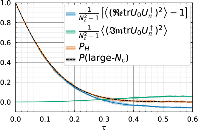
Figure 1: Gap survival probability (14) in $H\to gg$ with $\theta_{in}=\pi/3$ as a function of $\tau$. The large-$N_{c}$ result is constructed from the solution of (16) with $C_{F}=N_{c}/2$.

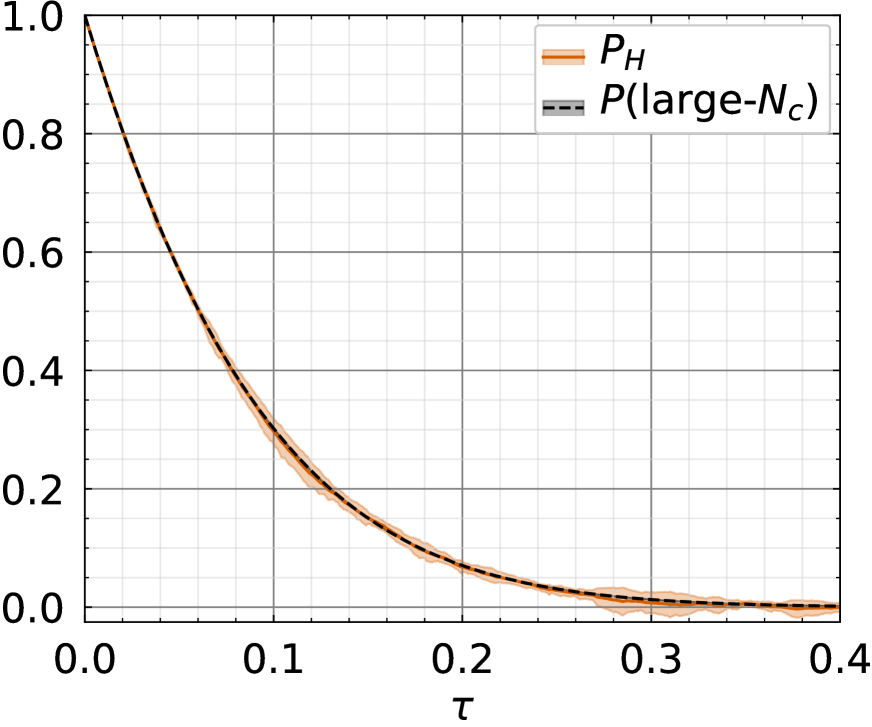
(a)

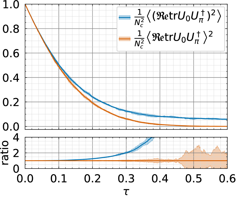
(b)

Figure 2: (a) Same as Fig. 1 except that here $\theta_{in}=\pi/4$; (b) Plots of the two terms in (15), both normalized to unity at $\tau=0$.

IV Jet veto in Higgs plus dijet production

We now turn our attention to the more interesting but difficult problem of hadron collisions with $2\to 2$ hard parton subprocesses. In this case, there are four primary partons (quarks or gluons) in the initial and final states, and the emission of soft gluons from this four-pronged antenna is obviously much more complicated than the previous examples. Nevertheless, the resummation of the Sudakov logarithms can be done (at finite-$N_{c}$) using the techniques of the soft anomalous dimension Kidonakis et al. (1998). The non-global logarithms are parametrically of the same order, but their resummation has been done only in the large-$N_{c}$ approximation for dijet production at the LHC Hatta et al. (2013). In this section, we perform, for the first time, the leading-logarithmic resummation of non-global logarithms for $2\to 2$ scatterings at finite-$N_{c}$, taking Higgs plus dijet production in $pp$ collisions at the LHC as a concrete example. We however have to sacrifice the super-leading logarithms which are relevant to the present problem since there are hard partons in both the initial and final states. We leave this to future work.

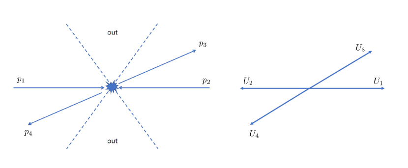
Figure 3: $2\to 2$ parton scattering with momentum assignments (left) and the corresponding antenna structure (right).

IV.1 $qq\to qqH$

Let us first consider the simplest channel $q_{i}(p_{1})q_{j}(p_{2})\to q_{k}(p_{3})q_{l}(p_{4})H$ where $i,j,k,l=1,2,3$ are color indices. The outgoing quarks (or antiquarks) with momenta $p_{3}$, $p_{4}$ are back-to-back and detected as two jets in the forward and backward directions, see Fig. 3. The radiation pattern is sensitive to how color flows in the $2\to 2$ scattering. Following Forshaw and Sjodahl (2007), we use the eikonal approximation $\bar{u}(p_{3})\gamma^{\mu}u(p_{1})\approx 2p^{\mu}_{1}$ and parameterize the leading-order amplitude as

$${\mathcal{M}}_{ijkl}=M_{1}\delta_{ki}\delta_{lj}+M_{8}t^{a}_{ki}t^{a}_{lj}=\left(M_{1}-\frac{M_{8}}{2N_{c}}\right)\delta_{ki}\delta_{lj}+\frac{M_{8}}{2}\delta_{kj}\delta_{li}.$$ (18)

The singlet $M_{1}$ and octet $M_{8}$ contributions are from the $Z$-boson fusion and the gluon-gluon fusion processes, respectively. Their explicit forms are not important for this work. They can be found in the literature Forshaw and Sjodahl (2007). The $W$-boson fusion amplitude does not interfere with the above amplitude because $W$’s have an electric charge. As far as the color structure is concerned, the $W$-fusion process is identical to the $Z$-boson case, and does not require a separate consideration.

We now dress up (18) by attaching soft gluons to external legs in the eikonal approximation. This converts (18) into

$${\mathcal{M}}^{\prime}_{ijkl}=\left(M_{1}-\frac{M_{8}}{2N_{c}}\right)(U_{3}U^{\dagger}_{1})_{ki}(U_{4}U^{\dagger}_{2})_{lj}+\frac{M_{8}}{2}(U_{3}U_{2}^{\dagger})_{kj}(U_{4}U_{1}^{\dagger})_{li}$$ (19)

We then square it and average over $ij$, and sum over $kl$

$$\frac{1}{N_{c}^{2}}\sum_{ijkl}|{\mathcal{M}}^{\prime}|^{2} = \frac{1}{N_{c}^{2}}\left|M_{1}-\frac{M_{8}}{2N_{c}}\right|^{2}{\rm tr}(U_{3}U^{\dagger}_{1}V_{1}V_{3}^{\dagger}){\rm tr}(U_{4}U^{\dagger}_{2}V_{2}V_{4}^{\dagger})+\frac{|M_{8}|^{2}}{4N_{c}^{2}}{\rm tr}(U_{3}U_{2}^{\dagger}V_{2}V_{3}^{\dagger}){\rm tr}(U_{4}U_{1}^{\dagger}V_{1}V_{4}^{\dagger})$$ (20)

$$+\left(M_{1}-\frac{M_{8}}{2N_{c}}\right)\frac{M_{8}^{*}}{2N_{c}^{2}}{\rm tr}(U_{3}U_{1}^{\dagger}V_{1}V_{4}^{\dagger}U_{4}U_{2}^{\dagger}V_{2}V_{3}^{\dagger})+(c.c.)$$

Using the fact that $M_{1}$ and $M_{8}$ are real and relabeling $V^{\dagger}U\to U$ (see (9)), we can write

$$\frac{1}{N_{c}^{2}}\sum_{ijkl}|{\mathcal{M}}^{\prime}|^{2} = \frac{1}{N_{c}^{2}}\left(M_{1}-\frac{M_{8}}{2N_{c}}\right)^{2}{\rm tr}(U_{3}U^{\dagger}_{1}){\rm tr}(U_{4}U^{\dagger}_{2})+\frac{M_{8}^{2}}{4N_{c}^{2}}{\rm tr}(U_{3}U_{2}^{\dagger}){\rm tr}(U_{4}U_{1}^{\dagger})$$ (21)

$$+\left(M_{1}-\frac{M_{8}}{2N_{c}}\right)\frac{M_{8}}{N_{c}^{2}}\mathfrak{Re}\Bigl{\{}{\rm tr}(U_{3}U_{1}^{\dagger}U_{4}U_{2}^{\dagger})\Bigr{\}}.$$

We see that the cross section involves products of color dipoles ${\rm tr}(UU^{\dagger}){\rm tr}(UU^{\dagger})$ and also a color quadrupole ${\rm tr}(UU^{\dagger}UU^{\dagger})$. We evaluated these multipoles for a back-to-back configuration $(\theta_{3},\phi_{3})=(\frac{\pi}{6},0)$ and $(\theta_{4},\phi_{4})=(\frac{5\pi}{6},\pi)$ with $\theta_{in}=\pi/3$. As before, we average over 3000 random walks on $80\times 60$ and $60\times 40$ lattices. The results are plotted in Fig. 4 with now

$$\tau=\frac{\alpha_{s}}{\pi}\ln\frac{P_{T}}{E_{out}},$$ (22)

where $P_{T}$ is the jet transverse momentum. Only the real parts are plotted. The imaginary parts are consistent with zero within errors.

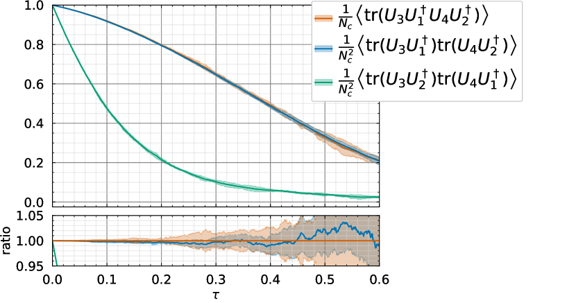
Figure 4: Color multipoles relevant to the gap survival probability in $qq\to qqH$, see (21). Only the real parts are plotted.

Surprisingly, we find, to a very good approximation,

$$\left\langle\frac{1}{N_{c}}{\rm tr}(U_{3}U_{1}^{\dagger}U_{4}U_{2}^{\dagger})\right\rangle\approx\left\langle\frac{1}{N_{c}^{2}}{\rm tr}(U_{3}U_{1}^{\dagger}){\rm tr}(U_{4}U_{2}^{\dagger})\right\rangle.$$ (23)

Namely, the color quadrupole factorizes into the product of color dipoles. We have checked that this property does not hold in each configuration, but emerges only after averaging over many events. [Note that (23) is trivially satisfied by the initial condition since $U=1$ everywhere.] It is surprising because such factorization has not been seen in the previous studies of color multipoles in the context of small-$x$ QCD, see e.g., Blaizot et al. (2004); Dominguez et al. (2011b); Dumitru et al. (2011); Shi et al. (2017). The lesson learned in these studies is that a quadrupole does not factorize into dipoles in general. And when it factorizes in some limit and in some sense, due to the cyclic property of trace, the two possible color singlet combinations ${\rm tr}(U_{3}U_{1}^{\dagger}){\rm tr}(U_{4}U_{2}^{\dagger})$ and ${\rm tr}(U_{2}^{\dagger}U_{3}){\rm tr}(U_{1}^{\dagger}U_{4})$ have to appear symmetrically. However, in (23) only the former appears. As shown in Fig. 4, the latter (green curve) is indeed numerically smaller since the dipoles have wider opening angles, but not negligibly smaller. While we do not understand the reason of this puzzling behavior, presumably it has to do with color coherence and angular ordering: Parton 3 prefers to pair up with parton 1 because then they can form a color-singlet dipole with a small opening angle ($\pi/6$ in this case) which is ‘protected’ from the 2-4 dipole in the backward direction. What is striking about (23) is that this tendency is pushed to the extreme. This point certainly deserves further studies. It is also interesting to see whether a relation analogous to (23) holds for any configuration of dipoles in the small-$x$ problem.

Let us now consider the implications of (23). We immediately notice that if we use (23) in (21), the interference term $\propto M_{1}M_{8}$ between the $Z$-boson and gluon fusion amplitudes vanishes. Actually, that the interference effect is numerically very small was already observed in Forshaw and Sjodahl (2007). Even without soft gluon emissions, it is already suppressed at the tree level due to a cancellation between contributions from different flavors and helicities. [$M_{1}$ depends on these quantum numbers.] Interestingly, in addition to this ‘accidental’ suppression, here we find another dynamical source of suppression which makes the interference term really small. After using the relation (23) in (21), we get

$$M_{1}^{2}P_{qq}^{1}+\frac{N_{c}^{2}-1}{4N_{c}^{2}}M_{8}^{2}P_{qq}^{8},$$ (24)

where the probabilities

$$P_{qq}^{1} \equiv \frac{1}{N_{c}^{2}}\left\langle{\rm tr}(U_{3}U_{1}^{\dagger}){\rm tr}(U_{4}U_{2}^{\dagger})\right\rangle,$$ (25)

$$P^{8}_{qq} \equiv \frac{1}{N_{c}^{2}-1}\left\langle{\rm tr}(U_{3}U_{2}^{\dagger}){\rm tr}(U_{4}U_{1}^{\dagger})-\frac{1}{N_{c}^{2}}{\rm tr}(U_{3}U_{1}^{\dagger}){\rm tr}(U_{4}U_{2}^{\dagger})\right\rangle,$$ (26)

are normalized to unity at $\tau=0$. In Fig. 5(a), we plot $P_{qq}^{1}$ together with its mean-field approximated version

$$P^{1}_{qq}({\rm MFA})\equiv\left\langle\frac{1}{N_{c}}{\rm tr}(U_{3}U_{1}^{\dagger})\right\rangle\left\langle\frac{1}{N_{c}}{\rm tr}(U_{4}U_{2}^{\dagger})\right\rangle.$$ (27)

as well as the large-$N_{c}$ version

$$P^{1}_{qq}(\text{large-}N_{c})\equiv P_{13}P_{24}$$ (28)

where $P_{\alpha\beta}$ is the solution of the BMS equation (16) with $C_{F}=\frac{N_{c}^{2}-1}{2N_{c}}=\frac{4}{3}$ (pink curve) and $C_{F}\approx\frac{N_{c}}{2}=\frac{3}{2}$ (black curve).

In Fig. 5(b), we plot $P_{qq}^{8}$ and its variants

$$P_{qq}^{8}(\text{large-}N_{c}+) \equiv \frac{1}{N_{c}^{2}}\left\langle{\rm tr}(U_{3}U_{2}^{\dagger}){\rm tr}(U_{4}U_{1}^{\dagger})\right\rangle,$$ (29)

$$P_{qq}^{8}({\rm MFA}) \equiv \left\langle\frac{1}{N_{c}}{\rm tr}(U_{3}U_{2}^{\dagger})\right\rangle\left\langle\frac{1}{N_{c}}{\rm tr}(U_{4}U_{1}^{\dagger})\right\rangle$$ (30)

$$P_{qq}^{8}(\text{large-}N_{c}) \equiv P_{23}P_{14}$$ (31)

(29) is obtained from $P_{qq}^{8}$ by keeping terms with the largest power of $N_{c}$ under the counting rules ${\rm tr}(UU^{\dagger})\sim{\rm tr}(UU^{\dagger}UU^{\dagger})\sim N_{c}$, $N_{c}^{2}-1\approx N_{c}^{2}$. For the lack of a better name, we refer to it as the ‘large-$N_{c}+$’ approximation, although it is a bit misleading since we evaluate the resulting expression fully at $N_{c}=3$. The ‘genuine’ large-$N_{c}$ approximation is given by (31) where $P_{\alpha\beta}$ is calculated from the BMS equation with $C_{F}=N_{c}/2$.

We immediately notice that the MFA $\langle AB\rangle\approx\langle A\rangle\langle B\rangle$ holds almost perfectly in Fig. 5(a) but fails completely in Fig. 5(b) for $\tau\gtrsim 0.2$ (compare the green and orange curves). Combining with the previous example Fig. 2(b), we can infer that the MFA is good when the two dipoles are far apart in solid angles, but violated when they are close to each other, see Fig. 3(right). This supports our previous claim that the breakdown of the MFA is due to the spatial correlation among soft gluons which gets stronger when they are close to each other Hatta and Mueller (2007); Avsar and Hatta (2008).

We next observe that, surprisingly, the full result (26) (blue curve in Fig. 5(b)) agrees almost perfectly with the large-$N_{c}$ result (31). This is similar to the relation $P_{H}\approx P(\text{large-}N_{c})$ found in the previous section, but unlike there, this time we do not have a simple explanation. [Note, however, that (26) reduces to (14) in the limits $\theta_{3}\to 0$, $\theta_{4}\to\pi$.] Our result indicates that the large suppression factor when going from (29) to (30) perfectly mimics the second term of (26) discarded in the large-$N_{c}$ approximation. Despite the explicit factor of $1/N_{c}^{2}$, the second term is not at all negligible compared to the first term when $\tau\gtrsim 0.2$. In fact, $P_{qq}^{8}$ vanishes around $\tau\sim 0.4$ due to an almost exact cancellation between the two terms. How can $P_{qq}^{8}(\text{large-}N_{c})$ know about this delicate cancellation when it totally ignores the 1-3 and 2-4 dipoles? An easy explanation is that the agreement is just an accident, but there may be a deep reason. We shall return to this issue later.

Finally, the large-$N_{c}$ approximation is violated in the singlet sector $P_{qq}^{1}$ (compare the blue and black curves in Fig. 5(a)). Actually, from our experience in Hatta and Ueda (2013), we expected the factorized product $P_{qq}^{1}(\text{MFA})$ to be very close to the solution of the BMS equation with $C_{F}=4/3$ (pink curve), but we see a clear deviation for $\tau>0.3$. While this may be physical, one has to be very careful about lattice artifacts. The 1-3 and 2-4 dipoles involved in the singlet channel have a small opening angle, and hence they may be more susceptible to lattice discretization errors. Besides, such errors are doubled when computing the square $P_{qq}^{1}\sim(P_{13})^{2}$. To settle this issue, we need simulations on much finer lattices, which is however computationally challenging in the present approach.

All these results are in stark contrast to the case of $e^{+}e^{-}$ annihilation where one does not see any unusual behavior at such early ‘times’ $\tau\sim 0.2$ Hatta and Ueda (2013); Hagiwara et al. (2016). In particular, the finite-$N_{c}$ corrections to the color dipole is quite small in this regime. In the corresponding small-$x$ problem, it has even been argued that the $1/N_{c}^{2}$ corrections are smaller by orders of magnitude than the naive expectation $1/N_{c}^{2}\sim 10$% Kovchegov et al. (2009). However, in hadron-hadron collisions, the gap survival probability $P_{hh}$ consists of higher multipoles and becomes small, say $P_{hh}<0.2$, already in the phenomenologically relevant region of $\tau$. In this region, naively subdominant effects (spatial correlations, finite-$N_{c}$) can give corrections of order unity. Barring further “accidents” to happen, it is simply best to avoid any approximations under such circumstances.

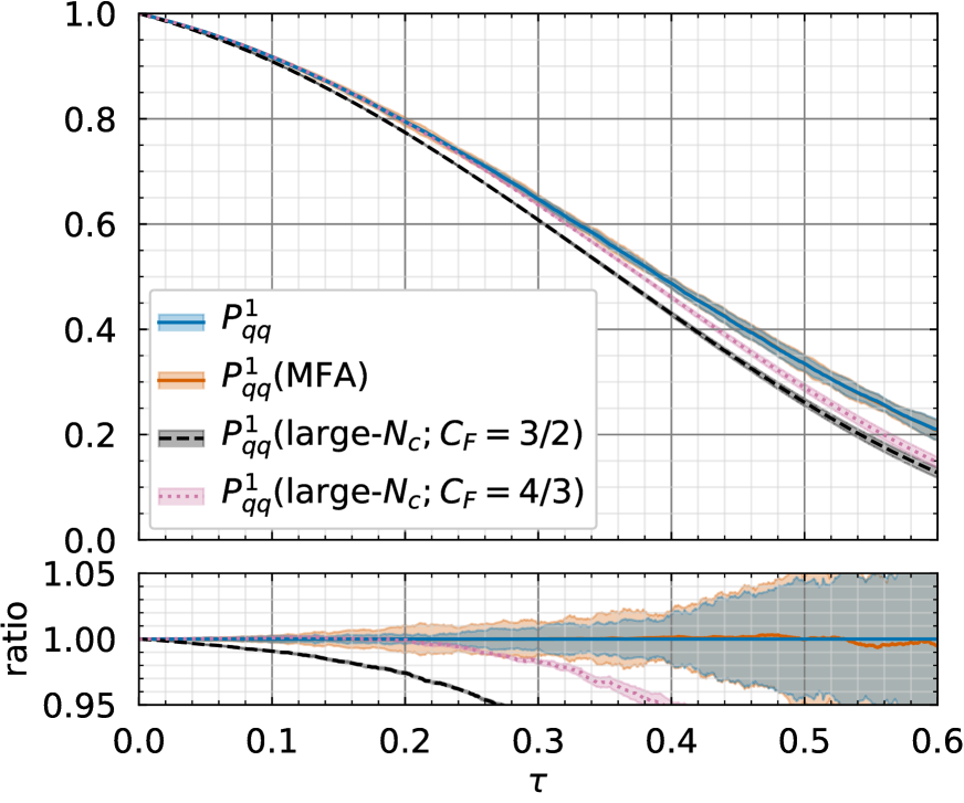
(a)

(b)

Figure 5: Gap survival probabilities in $qq\to qqH$, color-singlet (a) and color-octet (b) channels.

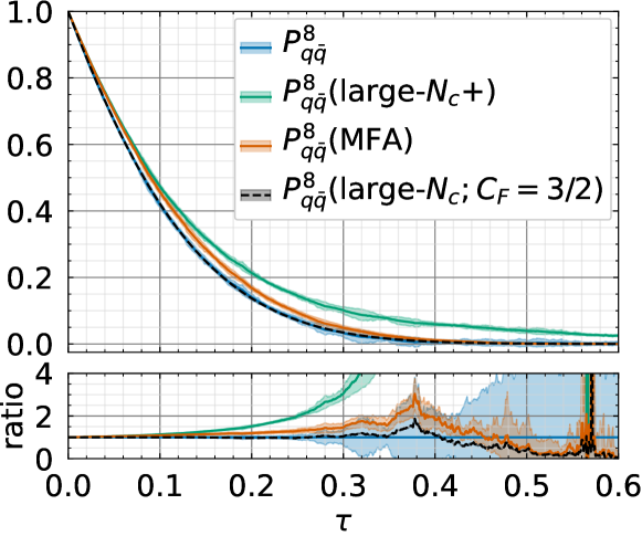
Figure 6: Gap survival probability in $q\bar{q}\to q\bar{q}$, octet channel (36).

IV.2 $q\bar{q}\to q\bar{q}H$

Next consider the channel $q\bar{q}\to q\bar{q}H$. In the eikonal approximation $\bar{v}(p_{2})\gamma^{\mu}v(p_{4})\approx 2p^{\mu}_{2}$, we write

$${\mathcal{M}}_{ijkl}=-M_{1}\delta_{ki}\delta_{lj}-M_{8}t^{a}_{ki}t^{a}_{jl}=-\left(M_{1}-\frac{M_{8}}{2N_{c}}\right)\delta_{ki}\delta_{lj}-\frac{M_{8}}{2}\delta_{kl}\delta_{ij},$$

$$\to{\mathcal{M}}_{ijkl}^{\prime}=-\left(M_{1}-\frac{M_{8}}{2N_{c}}\right)(U_{3}U_{1}^{\dagger})_{ki}(U_{2}U_{4}^{\dagger})_{jl}-\frac{M_{8}}{2}(U_{3}U_{4}^{\dagger})_{kl}(U_{2}U_{1}^{\dagger})_{ji}.$$ (32)

A minus sign is needed when replacing a quark with an antiquark. Squaring and averaging over color indices, we get

$$\frac{1}{N_{c}^{2}}\sum_{ijkl}|{\mathcal{M}}^{\prime}|^{2}=\frac{1}{N_{c}^{2}}\left(M_{1}-\frac{M_{8}}{2N_{c}}\right)^{2}{\rm tr}(U_{3}U_{1}^{\dagger}){\rm tr}(U_{2}U_{4}^{\dagger})+\frac{M_{8}^{2}}{4N_{c}^{2}}{\rm tr}(U_{3}U_{4}^{\dagger}){\rm tr}(U_{2}U_{1}^{\dagger})$$

$$+\left(M_{1}-\frac{M_{8}}{2N_{c}}\right)\frac{M_{8}}{N_{c}^{2}}\mathfrak{Re}\Bigl{\{}{\rm tr}(U_{3}U_{1}^{\dagger}U_{2}U_{4}^{\dagger})\Bigr{\}}.$$ (33)

We have checked that, similarly to (23),

$$\left\langle\frac{1}{N_{c}}{\rm tr}(U_{3}U_{1}^{\dagger}U_{2}U_{4}^{\dagger})\right\rangle\approx\left\langle\frac{1}{N_{c}^{2}}{\rm tr}(U_{3}U_{1}^{\dagger}){\rm tr}(U_{2}U_{4}^{\dagger})\right\rangle\approx\left\langle\frac{1}{N_{c}}{\rm tr}(U_{3}U_{1}^{\dagger}U_{4}U_{2}^{\dagger})\right\rangle,$$ (34)

so that again the interference term $\sim M_{1}M_{8}$ in (33) is negligibly small. Eq. (33) then reduces to

$$M_{1}^{2}P_{q\bar{q}}^{1}+\frac{N_{c}^{2}-1}{4N_{c}^{2}}M_{8}^{2}P^{8}_{q\bar{q}}$$ (35)

where $P_{q\bar{q}}^{1}\approx P_{qq}^{1}$ and

$$P^{8}_{q\bar{q}}\equiv\frac{1}{N_{c}^{2}-1}\left\langle{\rm tr}(U_{3}U_{4}^{\dagger}){\rm tr}(U_{2}U_{1}^{\dagger})-\frac{1}{N_{c}^{2}}{\rm tr}(U_{3}U_{1}^{\dagger}){\rm tr}(U_{2}U_{4}^{\dagger})\right\rangle.$$ (36)

This is plotted in Fig. 6 together with its three variants

$$P^{8}_{q\bar{q}}(\text{large-}N_{c}+) \equiv \frac{1}{N_{c}^{2}}\left\langle{\rm tr}(U_{3}U_{4}^{\dagger}){\rm tr}(U_{2}U_{1}^{\dagger})\right\rangle,$$ (37)

$$P^{8}_{q\bar{q}}({\rm MFA}) \equiv \left\langle\frac{1}{N_{c}}{\rm tr}(U_{3}U_{4}^{\dagger})\right\rangle\left\langle\frac{1}{N_{c}}{\rm tr}(U_{2}U_{1}^{\dagger})\right\rangle$$ (38)

$$P_{q\bar{q}}^{8}(\text{large-}N_{c};C_{F}=3/2) \equiv P_{34}P_{12}$$ (39)

As expected, the MFA does not hold for $\tau\gtrsim 0.2$ because the 3-4 and 1-2 dipoles are close in angles, see Fig. 3(right). Again the full result (36) agrees almost perfectly with the large-$N_{c}$ result (39) despite a series of approximations (36)$\to$(37)$\to$(38)$\to$(39) involved. Although nontrivial, this may not come as an additional surprise since the two processes $qq\to qq$ and $q\bar{q}\to q\bar{q}$ are rather similar in the present setup.

IV.3 $qg\to qgH$, $\bar{q}g\to\bar{q}gH$

Next we turn to the case which involves a gluon in the initial state $qg\to qgH$. ($\bar{q}g\to\bar{q}gH$ is entirely analogous and will be omitted.) There is no vector boson fusion contribution in this channel. The amplitude is given by

$${\mathcal{M}}^{ab}_{ik}=t^{c}_{ki}T^{c}_{ba}M_{8}\quad\to\quad{\mathcal{M}}^{\prime ab}_{ik}=(U_{3}t^{c}U^{\dagger}_{1})_{ki}(\tilde{U}_{4}T^{c}\tilde{U}_{2}^{\dagger})_{ba}M_{8},$$ (40)

where $a,b$ are the color indices of the initial and final gluons with $T^{c}_{ba}=-if_{cba}$. Squaring and averaging over color indices, we get

$$\frac{1}{N_{c}(N_{c}^{2}-1)}\sum_{ikab}|{\mathcal{M}}^{\prime}|^{2} = \frac{M_{8}^{2}}{N_{c}(N_{c}^{2}-1)}{\rm tr}(U_{3}t^{c}U_{1}^{\dagger}V_{1}t^{d}V_{3}^{\dagger}){\rm tr}(\tilde{U_{4}}T^{c}\tilde{U}_{2}^{\dagger}\tilde{V}_{2}T^{d}\tilde{V}^{\dagger}_{4})$$ (41)

$$\to \frac{M_{8}^{2}}{N_{c}(N_{c}^{2}-1)}{\rm tr}(t^{c}U^{\dagger}_{1}t^{d}U_{3}){\rm tr}(T^{c}\tilde{U}^{\dagger}_{2}T^{d}\tilde{U}_{4})$$

$$= \frac{M_{8}^{2}}{4N_{c}(N_{c}^{2}-1)}\biggl{(}{\rm tr}(U_{2}U^{\dagger}_{1}){\rm tr}(U_{3}U_{4}^{\dagger}){\rm tr}(U_{4}U_{2}^{\dagger})+{\rm tr}(U_{4}U_{1}^{\dagger}){\rm tr}(U_{2}U_{4}^{\dagger}){\rm tr}(U_{3}U_{2}^{\dagger})$$

$$\qquad\qquad-{\rm tr}(U_{4}U_{2}^{\dagger}U_{3}U_{4}^{\dagger}U_{2}U_{1}^{\dagger})-{\rm tr}(U_{4}U_{1}^{\dagger}U_{2}U_{4}^{\dagger}U_{3}U_{2}^{\dagger})\biggr{)}$$

$$\equiv\frac{M_{8}^{2}}{2}P_{qg}$$

We now have color sextupoles ${\rm tr}(UU^{\dagger}UU^{\dagger}UU^{\dagger})$ as well as products of three dipoles ${\rm tr}(UU^{\dagger}){\rm tr}(UU^{\dagger}){\rm tr}(UU^{\dagger})$. $P_{qg}$ is plotted in Fig. 7 together with its approximated versions

$$P_{qg}(\text{large-}N_{c}+)\equiv\frac{1}{2N_{c}^{3}}\left\langle{\rm tr}(U_{2}U^{\dagger}_{1}){\rm tr}(U_{3}U_{4}^{\dagger}){\rm tr}(U_{4}U_{2}^{\dagger})+{\rm tr}(U_{4}U_{1}^{\dagger}){\rm tr}(U_{2}U_{4}^{\dagger}){\rm tr}(U_{3}U_{2}^{\dagger})\right\rangle$$ (42)

$$P_{qg}({\rm MFA})\equiv\frac{1}{2}\left\langle\frac{{\rm tr}(U_{2}U_{1}^{\dagger})}{N_{c}}\right\rangle\left\langle\frac{{\rm tr}(U_{3}U_{4}^{\dagger})}{N_{c}}\right\rangle\left\langle\frac{{\rm tr}(U_{4}U_{2}^{\dagger})}{N_{c}}\right\rangle$$

$$\qquad\qquad\qquad\qquad+\frac{1}{2}\left\langle\frac{{\rm tr}(U_{4}U_{1}^{\dagger})}{N_{c}}\right\rangle\left\langle\frac{{\rm tr}(U_{2}U_{4}^{\dagger})}{N_{c}}\right\rangle\left\langle\frac{{\rm tr}(U_{3}U_{2}^{\dagger})}{N_{c}}\right\rangle$$ (43)

$$P_{qg}(\text{large-}N_{c};C_{F}=3/2)\equiv\frac{1}{2}(P_{12}P_{34}+P_{14}P_{23})P_{24}.$$ (44)

A priori, one would expect $P^{8}_{qq}\approx P^{8}_{q\bar{q}}>P_{qg}$, but their difference turns out to be numerically rather small. Fig. 7 looks almost the same as the previous plots. This is because, roughly,

$$P_{qg}\sim P_{41}P_{24}P_{32}\sim P_{24}P^{8}_{qq}$$ (45)

and $P_{24}$ is of order unity (for example, $P_{24}\approx 0.8$ when $\tau=0.3$). For the first time, we observe the large violation of the MFA in the three-dipole sector (green versus orange curves). The color sextupoles in (41) are nominally subleading $\sim{\cal O}(1/N_{c}^{2})$ in the $N_{c}$ counting, but they completely cancel the leading-$N_{c}$ terms for $\tau\gtrsim 0.3$. After this cancellation, once again, the exact result is very close to the large-$N_{c}$ result (44)!

IV.4 $gg\to ggH$

Finally, the amplitude in the $gg\to gg$ channel is

$${\mathcal{M}}_{aa^{\prime}bb^{\prime}}=M_{8}T^{c}_{ba}T^{c}_{b^{\prime}a^{\prime}}\quad\to\quad{\mathcal{M}}^{\prime}_{aa^{\prime}bb^{\prime}}=M_{8}(\tilde{U}_{3}T^{c}\tilde{U}_{1}^{\dagger})_{ba}(\tilde{U}_{4}T^{c}\tilde{U}_{2})_{b^{\prime}a^{\prime}}$$ (46)

Proceeding as before, we find

$$\frac{1}{(N_{c}^{2}-1)^{2}}\sum_{aa^{\prime}bb^{\prime}}|{\mathcal{M}}^{\prime}|^{2}$$

$$\to\frac{M_{8}^{2}}{(N_{c}^{2}-1)^{2}}{\rm tr}(T^{c}\tilde{U}^{\dagger}_{1}T^{d}\tilde{U}_{3}){\rm tr}(T^{c}\tilde{U}^{\dagger}_{2}T^{d}\tilde{U}_{4})$$

$$=\frac{M_{8}^{2}}{2(N_{c}^{2}-1)^{2}}\mathfrak{Re}\Biggl{\{}{\rm tr}(U_{1}U_{3}^{\dagger})\left({\rm tr}(U_{2}U_{4}^{\dagger}){\rm tr}(U_{4}U_{1}^{\dagger}){\rm tr}(U_{3}U_{2}^{\dagger})+{\rm tr}(U_{4}U_{2}^{\dagger}){\rm tr}(U_{2}U_{1}^{\dagger}){\rm tr}(U_{3}U_{4}^{\dagger})\right)$$

$$\qquad\qquad\qquad\qquad-{\rm tr}(U_{1}U_{3}^{\dagger})\left({\rm tr}(U_{4}U_{2}^{\dagger}U_{3}U_{4}^{\dagger}U_{2}U_{1}^{\dagger})+{\rm tr}(U_{2}U_{4}^{\dagger}U_{3}U_{2}^{\dagger}U_{4}U_{1}^{\dagger})\right)$$

$$\qquad\qquad\qquad\qquad-{\rm tr}(U_{2}U_{4}^{\dagger})\left({\rm tr}(U_{1}U_{3}^{\dagger}U_{4}U_{1}^{\dagger}U_{3}U_{2}^{\dagger})+{\rm tr}(U_{3}U_{1}^{\dagger}U_{4}U_{3}^{\dagger}U_{1}U_{2}^{\dagger})\right)$$

$$\qquad\qquad\qquad\qquad+{\rm tr}(U_{3}U_{2}^{\dagger}U_{4}U_{1}^{\dagger}){\rm tr}(U_{2}U_{4}^{\dagger}U_{1}U_{3}^{\dagger})+{\rm tr}(U_{1}U_{2}^{\dagger}U_{4}U_{3}^{\dagger}){\rm tr}(U_{2}U_{4}^{\dagger}U_{3}U_{1}^{\dagger})\Biggr{\}}$$

$$\equiv\frac{N_{c}^{2}}{N_{c}^{2}-1}M_{8}^{2}P_{gg}.$$ (47)

This features various color multipoles consisting of eight Wilson lines. [Note that it does not contain ‘color octupoles’ ${\rm tr}(UU^{\dagger}UU^{\dagger}UU^{\dagger}UU^{\dagger})$.] $P_{gg}$ is plotted in Fig. 8 together with its three approximations

$$P_{gg}(\text{large-}N_{c}+)\equiv\frac{1}{2N_{c}^{4}}\left\langle{\rm tr}(U_{1}U_{3}^{\dagger})\left({\rm tr}(U_{2}U_{4}^{\dagger}){\rm tr}(U_{4}U_{1}^{\dagger}){\rm tr}(U_{3}U_{2}^{\dagger})+{\rm tr}(U_{4}U_{2}^{\dagger}){\rm tr}(U_{2}U_{1}^{\dagger}){\rm tr}(U_{3}U_{4}^{\dagger})\right)\right\rangle$$ (48)

$$P_{gg}({\rm MFA})\equiv\frac{1}{2}\left\langle\frac{{\rm tr}(U_{1}U^{\dagger}_{3})}{N_{c}}\right\rangle\Biggl{\{}\left\langle\frac{{\rm tr}(U_{2}U^{\dagger}_{4})}{N_{c}}\right\rangle\left\langle\frac{{\rm tr}(U_{4}U^{\dagger}_{1})}{N_{c}}\right\rangle\left\langle\frac{{\rm tr}(U_{3}U^{\dagger}_{2})}{N_{c}}\right\rangle$$

$$\qquad\qquad\qquad\qquad+\left\langle\frac{{\rm tr}(U_{4}U^{\dagger}_{2})}{N_{c}}\right\rangle\left\langle\frac{{\rm tr}(U_{2}U^{\dagger}_{1})}{N_{c}}\right\rangle\left\langle\frac{{\rm tr}(U_{3}U^{\dagger}_{4})}{N_{c}}\right\rangle\Biggr{\}}$$ (49)

$$P_{gg}(\text{large-}N_{c};C_{F}=3/2)\equiv\frac{1}{2}P_{13}P_{24}(P_{14}P_{23}+P_{12}P_{34}).$$ (50)

By now the pattern is routine. The MFA is violated also in the four-dipole sector, and the terms that consist of higher multipoles are not negligible compared to the leading-$N_{c}$, dipole terms. Nevertheless, the final result is very well approximated by the large-$N_{c}$ result (50) with $C_{F}=3/2$.

At this point, we must abandon the idea that the agreement between the full-$N_{c}$ and large-$N_{c}$ results is accidental. Actually, we have also tried asymmetric jets configurations such as $(\theta_{3},\theta_{4})=(15^{\rm o},150^{\rm o})$ and $(45^{\rm o},150^{\rm o}$) and arrived at the same conclusion. This is a striking observation. We would have expected that $P(\text{large-}N_{c})$ would be the worst approximation of all. Indeed, the naively subleading terms in $N_{c}$ are numerically significant and push the green curve down to the blue curve. Yet, the large-$N_{c}$ approximation somehow ‘knows’ this cancellation in advance, and gives almost correct results in terms of most simplistic formulas. How this is possible is unclear to us.

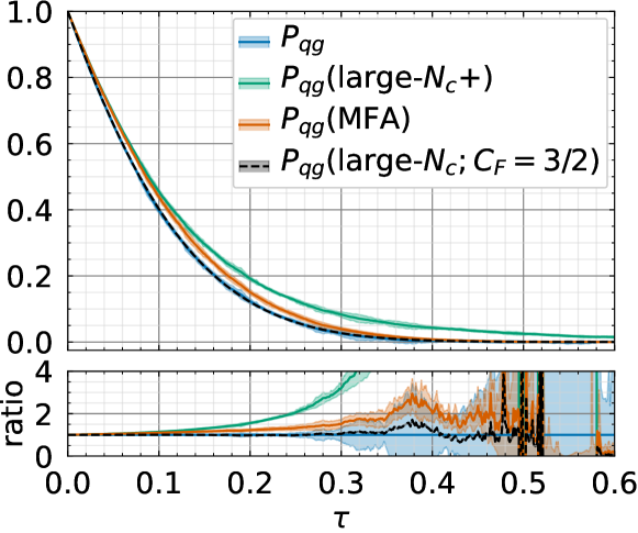
Figure 7: Gap survival probability in the $qg\to qg$ channel.

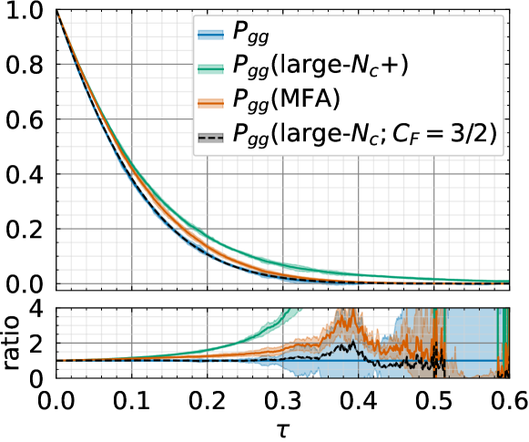
Figure 8: Gap survival probability in the $gg\to gg$ channel.

V Conclusions

In this paper, we have performed the resummation of leading non-global logarithms for two specific observables in proton-proton collisions at the LHC. No approximation is used for the number of colors $N_{c}=3$. In contrast to $e^{+}e^{-}$ annihilation studied previously, higher order color multipoles come into play. They can be straightforwardly evaluated in our formalism developed in Hatta and Ueda (2013). Our simulations have revealed several surprising features, such as the reduction of a quadrupole into the product of dipoles (23) and the failure of the ‘large-$N_{c}+$’ and mean field approximations. In particular, terms naively subleading in $N_{c}$ can completely cancel the leading-$N_{c}$ terms when $\tau\gtrsim 0.3$.

The final surprise is that, despite these highly nontrivial finite-$N_{c}$ effects, the large-$N_{c}$ result $P(\text{large-}N_{c})$ with $C_{F}=3/2$, which naively appears to be the least precise approximation, agrees perfectly with the exact $N_{c}=3$ result at least up to $\tau\sim 0.3$. We have confirmed this in all the subprocesses studied in this paper except in the singlet channel $P_{qq}^{1}$. In $H\to gg$, there is a semi-analytical explanation of how this might occur (see the paragraph below (17)), but for the dijet case, at the moment we do not understand why this should be the case. A close inspection of the leading order Sudakov ${\cal O}(\alpha_{s})$ and non-global ${\cal O}(\alpha_{s}^{2})$ logarithms in $2\to 2$ processes may help resolve this issue.

It remains to be seen whether a similar conclusion holds for other observables. Even for the dijet problem, a number of tests can be carried out. For example, one can relax the eikonal approximation used to derive (18), cf., Hatta et al. (2013), or one can use different definitions of the ‘out’ region. We leave this to future work. If, after all these tests, the relation $P(N_{c}=3)\approx P(\text{large-}N_{c})$ turns out to be robust, it is good news because one can approximately get full-$N_{c}$ results in hadron collisions using the known large-$N_{c}$ frameworks Dasgupta and Salam (2001, 2002); Banfi et al. (2002).

References

- Platzer and Sjodahl (2012) S. Platzer and M. Sjodahl, JHEP 07, 042 (2012), arXiv:1201.0260 [hep-ph] .
- Nagy and Soper (2015) Z. Nagy and D. E. Soper, JHEP 07, 119 (2015), arXiv:1501.00778 [hep-ph] .
- Dasgupta et al. (2018) M. Dasgupta, F. A. Dreyer, K. Hamilton, P. F. Monni, and G. P. Salam, JHEP 09, 033 (2018), [Erratum: JHEP 03, 083 (2020)], arXiv:1805.09327 [hep-ph] .
- Forshaw et al. (2019) J. R. Forshaw, J. Holguin, and S. Plätzer, JHEP 08, 145 (2019), arXiv:1905.08686 [hep-ph] .
- Nagy and Soper (2019) Z. Nagy and D. E. Soper, Phys. Rev. D 100, 074005 (2019), arXiv:1908.11420 [hep-ph] .
- Höche and Reichelt (2020) S. Höche and D. Reichelt, (2020), arXiv:2001.11492 [hep-ph] .
- Dasgupta et al. (2020) M. Dasgupta, F. A. Dreyer, K. Hamilton, P. F. Monni, G. P. Salam, and G. Soyez, Phys. Rev. Lett. 125, 052002 (2020), arXiv:2002.11114 [hep-ph] .
- Balsiger et al. (2020) M. Balsiger, T. Becher, and A. Ferroglia, JHEP 09, 029 (2020), arXiv:2006.00014 [hep-ph] .
- Angelis et al. (2020) M. D. Angelis, J. R. Forshaw, and S. Plätzer, (2020), arXiv:2007.09648 [hep-ph] .
- Hamilton et al. (2020) K. Hamilton, R. Medves, G. P. Salam, L. Scyboz, and G. Soyez, (2020), arXiv:2011.10054 [hep-ph] .
- Höche (2015) S. Höche, in Theoretical Advanced Study Institute in Elementary Particle Physics: Journeys Through the Precision Frontier: Amplitudes for Colliders (2015) pp. 235–295, arXiv:1411.4085 [hep-ph] .
- Dasgupta and Salam (2001) M. Dasgupta and G. Salam, Phys. Lett. B 512, 323 (2001), arXiv:hep-ph/0104277 .
- Dasgupta and Salam (2002) M. Dasgupta and G. P. Salam, JHEP 03, 017 (2002), arXiv:hep-ph/0203009 .
- Banfi et al. (2002) A. Banfi, G. Marchesini, and G. Smye, JHEP 08, 006 (2002), arXiv:hep-ph/0206076 .
- Hatta and Ueda (2013) Y. Hatta and T. Ueda, Nucl. Phys. B 874, 808 (2013), arXiv:1304.6930 [hep-ph] .
- Weigert (2004) H. Weigert, Nucl. Phys. B 685, 321 (2004), arXiv:hep-ph/0312050 .
- Hatta (2008) Y. Hatta, JHEP 11, 057 (2008), arXiv:0810.0889 [hep-ph] .
- Caron-Huot (2018) S. Caron-Huot, JHEP 03, 036 (2018), arXiv:1501.03754 [hep-ph] .
- Neill and Ringer (2020) D. Neill and F. Ringer, JHEP 06, 086 (2020), arXiv:2003.02275 [hep-ph] .
- Blaizot et al. (2003) J.-P. Blaizot, E. Iancu, and H. Weigert, Nucl. Phys. A 713, 441 (2003), arXiv:hep-ph/0206279 .
- Hagiwara et al. (2016) Y. Hagiwara, Y. Hatta, and T. Ueda, Phys. Lett. B 756, 254 (2016), arXiv:1507.07641 [hep-ph] .
- Hatta et al. (2013) Y. Hatta, C. Marquet, C. Royon, G. Soyez, T. Ueda, and D. Werder, Phys. Rev. D 87, 054016 (2013), arXiv:1301.1910 [hep-ph] .
- Hatta and Ueda (2009) Y. Hatta and T. Ueda, Phys. Rev. D 80, 074018 (2009), arXiv:0909.0056 [hep-ph] .
- Balitsky (1996) I. Balitsky, Nucl. Phys. B 463, 99 (1996), arXiv:hep-ph/9509348 .
- Kovchegov et al. (2009) Y. V. Kovchegov, J. Kuokkanen, K. Rummukainen, and H. Weigert, Nucl. Phys. A 823, 47 (2009), arXiv:0812.3238 [hep-ph] .
- Dominguez et al. (2011a) F. Dominguez, A. Mueller, S. Munier, and B.-W. Xiao, Phys. Lett. B 705, 106 (2011a), arXiv:1108.1752 [hep-ph] .
- Dumitru et al. (2011) A. Dumitru, J. Jalilian-Marian, T. Lappi, B. Schenke, and R. Venugopalan, Phys. Lett. B 706, 219 (2011), arXiv:1108.4764 [hep-ph] .
- Marquet et al. (2016) C. Marquet, E. Petreska, and C. Roiesnel, JHEP 10, 065 (2016), arXiv:1608.02577 [hep-ph] .
- Forshaw et al. (2006) J. R. Forshaw, A. Kyrieleis, and M. Seymour, JHEP 08, 059 (2006), arXiv:hep-ph/0604094 .
- Forshaw et al. (2008) J. Forshaw, A. Kyrieleis, and M. Seymour, JHEP 09, 128 (2008), arXiv:0808.1269 [hep-ph] .
- Mueller and Patel (1994) A. H. Mueller and B. Patel, Nucl. Phys. B 425, 471 (1994), arXiv:hep-ph/9403256 .
- Hatta and Mueller (2007) Y. Hatta and A. Mueller, Nucl. Phys. A 789, 285 (2007), arXiv:hep-ph/0702023 .
- Avsar and Hatta (2008) E. Avsar and Y. Hatta, JHEP 09, 102 (2008), arXiv:0805.0710 [hep-ph] .
- Avsar et al. (2009) E. Avsar, Y. Hatta, and T. Matsuo, JHEP 06, 011 (2009), arXiv:0903.4285 [hep-ph] .
- Kidonakis et al. (1998) N. Kidonakis, G. Oderda, and G. F. Sterman, Nucl. Phys. B 531, 365 (1998), arXiv:hep-ph/9803241 .
- Forshaw and Sjodahl (2007) J. R. Forshaw and M. Sjodahl, JHEP 09, 119 (2007), arXiv:0705.1504 [hep-ph] .
- Blaizot et al. (2004) J. P. Blaizot, F. Gelis, and R. Venugopalan, Nucl. Phys. A 743, 57 (2004), arXiv:hep-ph/0402257 .
- Dominguez et al. (2011b) F. Dominguez, C. Marquet, B.-W. Xiao, and F. Yuan, Phys. Rev. D 83, 105005 (2011b), arXiv:1101.0715 [hep-ph] .
- Shi et al. (2017) Y. Shi, C. Zhang, and E. Wang, Phys. Rev. D 95, 116014 (2017), arXiv:1704.00266 [hep-th] .