Variationally optimized orbital approach to trions in two-dimensional materials

Abstract

In this work, trions in two-dimensional (2D) space are studied by variational method with trial wavefunctions being constructed by linear combinations of 2D slater-type orbitals (STOs). Via this method, trion energy levels and wavefunctions can be calculated efficiently with fairly good accuracy. We first apply this method to study trion energy levels in a 2D hydrogen-like system with respect to a wide range of mass ratios and screening lengths. We find that the ground-state trion is bound for the whole parameter range, and an excited-state trion with antisymmetric permutation of electrons with finite angular momentum is bound for large electron-hole mass ratios or long screening lengths. The binding energies of ground-state trions calculated by the present method agree well with those calculated by more sophisticated but computationally-demanding methods. We then calculate trion states in various monolayer transition metal dichalcogenides (TMDCs) by using this method with the inclusion of electron-hole exchange (EHX) interaction. For TMDCs, we found that the effect of EHX can be significant in determining the trion binding energy and the possible existence of stable excited-state trions.

I Introduction

Excitonic complexes are known to be important components in determining the optical properties of low-dimensional semiconducting materials with direct bandgaps. A trion is a bound state of an exciton with another charged carrier which can either be an electron or hole. The former is called negative trion (or negatively charged exciton), and the latter is called positive trion (or positively charged exciton). Trions were observed initially in quantum-well systemskheng1993observation ; huard2000bound . In recent years, it was found that trion signatures appear frequently in the optical spectroscopy of two-dimensional (2D) materials due to their reduced dielectric screening that leads to greatly enhanced trion binding.mak2013tightly ; Lin Such an unique situation makes 2D materials a fertile playing ground for studying many-body physics. This subject has also attracted a great deal of theoretical interestsberkelbach2013theory ; berkelbach2017optical ; durnev2018excitons . Albeit many theoretical studies have been done, a refined theoretical work on this topic is still desired to explain emerging experimental observations and make better predictions.

To study the physical properties of trions in 2D materials, it is a prerequisite to know wavefunctions and energy levels. There are three frequently-used methodologies to calculate the trion wavefunctions in two dimensions: diagonalization of discretized trion Hamiltonianesser2000photoluminescence ; druppel2017diversity ; torche2019first ; tempelaar2019many ; zhumagulov2020three ; zhumagulov2020trion , quantum Monte Carlomayers2015binding ; kylanpaa2015binding ; velizhanin2015excitonic ; szyniszewski2017binding ; mostaani2017diffusion , and basis-function expansionphelps1983ground ; stebe1989ground ; usukura1999stability ; ruan2000application ; redlinski2001variational ; hilico2002quantum ; kidd2016binding ; van2017excitons ; hichri2017dielectric ; van2018excitons ; filikhin2018trions ; kezerashvili2017trion ; hichri2019charged ; jan2020excited . The first methodology includes the diagonalization of discretized three-particle Schrödinger equation in real spaceesser2000photoluminescence and discretized three-particle Bethe-Salpeter equation in momentum spacedruppel2017diversity ; torche2019first ; tempelaar2019many ; zhumagulov2020three ; zhumagulov2020trion . Both methods are useful to calculate trion energy levels but also numerically expansive to approach converged solutions. The second methodology is considered to be accurate in solving the ground-state wavefunction of a trion but difficult to be used in finding excited-state wavefunctions. The third methodology has several variants based on different basis functions used. An example of the methodology is to use a Hylleraas variational wavefunctionphelps1983ground ; stebe1989ground . The method can be vary accurate and efficient for calculating the ground-state energy of a trion. Another basis-function approach is to use Slater-type orbitals (STOs) to expand trion wavefunctionsredlinski2001variational ; hichri2017dielectric ; hichri2019charged . The method is quite nature for quantum chemists since a trion can be paralleled to a hydrogen ion ($H_{2}^{+}$ or $H^{-}$). Other examples include 2D harmonics in complex coordinatehilico2002quantum and hyperspherical harmonicsruan2000application ; kezerashvili2017trion ; filikhin2018trions . However, for a more complicated potential such as the Rytova-Keldysh potentialrytova ; Keldysh , it becomes difficult to calculate two-particle integrals efficiently. One who already overcomes the problem is the explicitly correlated Gaussian basis method, which is commonly used in stochastic variational methodusukura1999stability ; kidd2016binding ; van2017excitons ; van2018excitons ; jan2020excited . However, because the Gaussian basis does not describe the exponential asymptotic behavior of wavefunctions in the current system, the calculation requires a large number of basis functions and thus remains computationally intensive.

While all methods mentioned above are successfully in some degrees in finding a good ground-state trion, they may not be easily extended to the study of excited-state trions. In particular, it is difficult to verify whether an excited-state trion with nonzero angular momentum is bound, since the nodal structures and cusp conditions of excited-state wavefunctions are more sophisticated than ground-state wavefunctionskato1957eigenfunctions ; scott2007nodal . To study excited-state trions with nonzero angular momenta, a proper set of basis functions is needed to be carefully chosen to resemble the trion wavefunctions. STOs as basis functions are known for applications in quantum chemistry and atomic physicszener1930analytic ; levine2009quantum . Recently, 2D STOs are also used as basis functions to study exciton energy levels in 2D materialswu2019exciton ; henriques2020excitons ; quintela2020colloquium . In those studies, it is shown that the exciton energy levels can be calculated accurately by a variationally optimized procedure. Additionally, the asymptotic behavior of STOs is known to match that of wavefunctions in few-particle Coulombic systems in long distance and near two-particle coalescence points kato1957eigenfunctions . Therefore, STOs are preferred basis functions for studying low-lying states of trions. Furthermore, these STO basis functions have a common center that makes it easy to include the effect of Fermi-sea blockingchang2018crossover for electrically gated 2D materials which have become the desired experimental setup for such studiesmak2013tightly .

In this work, we use 2D STOs as basis functions to expand exciton and trion wavefunctions. We apply this procedure to the calculations of exciton and trion energy levels in two dimensions. Electron-electron and electron-hole interactions in two dimensions are modeled by Rytova-Keldysh potentialrytova ; Keldysh with an adjustable screening length, such that the present calculation can be used to simulate trion binding energies of transition metal dichalcogenide (TMDC) monolayers and benchmark with the binding energy of a 2D hydrogen ion. Two-particle integrals are computed by performing numerical integration over the Fourier transform of STOs and the Rytova-Keldysh potentialchang2018crossover . By this method, we can calculate trion energy levels efficiently and accurately in wide ranges of electron-hole mass ratios and screening lengths. For TMDCs, we found that the electron-hole exchange (EHX) interactionehx plays an important role in determining the trion binding energy. With the the inclusion of the EHX interaction, our calculation shows significant difference in trion binding energies associated with dark and bright excitons in WSe₂, which agrees with the experimental observation.

The article is organized as follows. In Sec. II, we first review the exciton and trion Hamiltonians and define the STO basis functions used. We also discuss how to implement the EHX term for TMDCs. In Sec. III, we provide the calculations of exciton and trion energy levels with respect to different mass ratios and screening lengths. Trion binding energies of TMDCs are also calculated and listed. A conclusion is given in Sec. IV. Details of the formulation for the variationally optimized orbital approach are given in Appendix.

II Theory

We briefly introduce exciton and trion Hamiltonians and introduce their corresponding wavefunctions and symmetries in Sec. II.1. The variationally optimized orbital approach to exciton and trion wavefunctions is delineated in Sec. II.2. The implementation of EHX corrections to the exciton and trion Hamiltonians is described in Sec. II.3.

II.1 Exciton and trion models

Based on effective mass approximation, excitons can be modeled by an exciton Hamiltonian ($\mathcal{H}_{\text{X}}$) composed of kinetic energy of an electron and a hole, and the electron-hole interaction given by a screened Coulomb potential.

$$\mathcal{H}_{\text{X}} = \frac{|\mathbf{p}_{\text{e}}|^{2}}{2m_{\text{e}}}+\frac{|\mathbf{p}_{\text{h}}|^{2}}{2m_{\text{h}}}-{V}(|\mathbf{r}_{\text{e}}-\mathbf{r}_{\text{h}}|),$$ (1)

where $\mathbf{r}_{e}$ ($\mathbf{r}_{h}$) denotes the coordinate of the electron (hole), $\mathbf{p}_{i}=-\mathtt{i}\hbar\bm{\nabla}_{i}$ is the momentum conjugate to $\mathbf{r}_{i}$ ($i=e,h$), and $m_{\text{e}}$ ($m_{\text{h}}$) is the effective mass of the electron (hole). $V(r)$ is the 2D screened Coulomb potential described by the Rytova-Keldysh potentialrytova ; Keldysh ,

$$V(r) = \frac{\pi e^{2}}{\kappa\rho_{0}}\left[H_{0}\left(\frac{r}{\rho_{0}}\right)-Y_{0}\left(\frac{r}{\rho_{0}}\right)\right]$$ (2)

$$= \int\;e^{\mathtt{i}\mathbf{k}\cdot\mathbf{r}}\left[\frac{2\pi e^{2}}{\kappa|\mathbf{k}|\left(1+|\mathbf{k}|\rho_{0}\right)}\right]\frac{\text{d}^{2}k}{(2\pi)^{2}},$$

where $\rho_{0}=r_{0}/\kappa$, $\kappa$ is the effective dielectric constant of the host material that includes the effect of the surrounding and $r_{0}$ is the screening length of the 2D material. $H_{0}(r)$ and $Y_{0}(r)$ are the Struve function and the Bessel function of the second kind. The second line in Eq. (2)gives the Fourier transform of the potential. The Rytova-Keldysh potential reduces to the Coulomb potential $V(r)\sim e^{2}/({\kappa r})$ in the long range limit ($r\gg\rho_{0}$), and in the short-range limit ($r\ll\rho_{0}$) it becomes a logarithmic potential $V(r)\sim[e^{2}/(\rho_{0}\kappa)]\left[\ln({2\rho_{0}}/{r})-\gamma\right]$ with $\gamma$ being the Euler’s constantmayers2015binding ; quintela2020colloquium . The Rytova-Keldysh potential is known for its appropriate description of the dielectric screening effect on 2D Coulomb potential and its accurate simulation of excitons and trions in various computational studiesmayers2015binding ; kylanpaa2015binding ; velizhanin2015excitonic ; kidd2016binding ; szyniszewski2017binding ; mostaani2017diffusion ; van2017excitons ; zhumagulov2020three ; zhumagulov2020trion ; jan2020excited ; quintela2020colloquium . Similarly, negative trions can be modeled by a trion Hamiltonian composed of kinetic energies of two electrons and one hole, and the screened Coulomb interaction among them

$$\mathcal{H}_{\text{T}} = \frac{|\mathbf{p}_{\text{e}1}|^{2}}{2m_{\text{e}}}+\frac{|\mathbf{p}_{\text{e}2}|^{2}}{2m_{\text{e}}}+\frac{|\mathbf{p}_{\text{h}}|^{2}}{2m_{\text{h}}}-{V}(|\mathbf{r}_{\text{e}1}-\mathbf{r}_{\text{h}}|)$$ (3)

$$-{V}(|\mathbf{r}_{\text{e}2}-\mathbf{r}_{\text{h}}|)+{V}(|\mathbf{r}_{\text{e}1}-\mathbf{r}_{\text{e}2}|),$$

The Hamiltonian for positive trions can be obtained by an exchange of the electron effective mass and hole effective mass in the Hamiltonian.

The exciton Hamiltonian becomes separable after making a transformation in terms of the center-of-mass (CM) coordinates $(\mathbf{R}_{\text{X}})$ and relative coordinates $(\mathbf{r})$. We have

$$\mathbf{R}_{\text{X}} = \frac{m_{\text{e}}\mathbf{r}_{\text{e}}+m_{\text{h}}\mathbf{r}_{\text{h}}}{m_{\text{X}}}\hskip 4.30554pt\mbox{and}\hskip 4.30554pt\mathbf{r}=\mathbf{r}_{\text{e}}-\mathbf{r}_{\text{h}},$$ (4)

where $m_{\text{X}}=m_{\text{e}}+m_{\text{h}}$ is the exciton total mass. The conjugate momenta for electron and hole can be written as

$$\mathbf{p}_{\text{e}}=\frac{m_{\text{e}}}{m_{\text{X}}}\mathbf{P}_{\text{X}}+\mathbf{p}\hskip 4.30554pt\mbox{and}\hskip 4.30554pt\mathbf{p}_{\text{h}}=\frac{m_{\text{h}}}{m_{\text{X}}}\mathbf{P}_{\text{X}}-\mathbf{p},$$ (5)

where $\mathbf{P}_{X}$ denotes the CM momentum and $\mathbf{p}$ is the momentum for the electron-hole relative motion in exciton. Similarly, the trion CM and relative coordinates are given by

$$\mathbf{R}_{\text{T}} = \frac{m_{\text{e}}\left(\mathbf{r}_{\text{e}1}+\mathbf{r}_{\text{e}2}\right)+m_{\text{h}}\mathbf{r}_{\text{h}}}{m_{\text{T}}},$$ (6)

$$\mathbf{r}_{1}=\mathbf{r}_{\text{e}1}-\mathbf{r}_{\text{h}},\hskip 4.30554pt\mbox{and}\hskip 4.30554pt\mathbf{r}_{2}=\mathbf{r}_{\text{e}2}-\mathbf{r}_{\text{h}}.$$ (7)

The coordinate transformation leads to the following relations for the conjugate momenta

$$\mathbf{p}_{\text{e}1}=\frac{m_{\text{e}}}{m_{\text{T}}}\mathbf{P}_{\text{T}}+\mathbf{p}_{1},\hskip 4.30554pt\mathbf{p}_{\text{e}2}=\frac{m_{\text{e}}}{m_{\text{T}}}\mathbf{P}_{\text{T}}+\mathbf{p}_{2},$$ (8)

$$\mathbf{p}_{\text{h}}=\frac{m_{\text{h}}}{m_{\text{T}}}\mathbf{P}_{\text{T}}-\mathbf{p}_{1}-\mathbf{p}_{2},$$ (9)

where $m_{\text{T}}=2m_{\text{e}}+m_{\text{h}}$ is the trion total mass. By inserting the transformed coordinates into the Hamiltonians, we see that the CM coordinates in both the exciton and the trion do not interact with the internal coordinates and can be neglected in the calculations of the energy levels. With the CM coordinates being disregarded the exciton and trion Hamiltonians can be written as

$$\mathcal{H}_{\text{X}}(\mathbf{r}) = -\frac{\hbar^{2}\nabla^{2}}{2\mu_{\text{X}}}-V(r),$$ (10)

$$\mathcal{H}_{\text{T}}(\mathbf{r}_{1},\mathbf{r}_{2}) = \mathcal{H}_{\text{X}}(\mathbf{r}_{1})+\mathcal{H}_{\text{X}}(\mathbf{r}_{2})-\frac{\hbar^{2}\bm{\nabla}_{1}\cdot\bm{\nabla}_{2}}{m_{\text{h}}}+V(r_{12}),$$

where $r_{12}=|\mathbf{r}_{1}-\mathbf{r}_{2}|$ and $\mu_{\text{X}}=(m_{\text{e}}m_{\text{h}})/(m_{\text{e}}+m_{\text{h}})$ is the exciton reduced mass. Given the exciton and trion Hamiltonians, the exciton and trion wavefunctions and eigenenergies can be solved from Schrödinger equations $\mathcal{H}_{\text{X}}(\mathbf{r})\Psi_{\text{X}}(\mathbf{r})=\varepsilon_{\text{X}}\Psi_{\text{X}}(\mathbf{r})$ and $\mathcal{H}_{\text{T}}(\mathbf{r}_{1},\mathbf{r}_{2})\Psi_{\text{T}}(\mathbf{r}_{1},\mathbf{r}_{2})=\varepsilon_{\text{T}}\Psi_{\text{T}}(\mathbf{r}_{1},\mathbf{r}_{2})$, where $\Psi_{\text{X}}(\mathbf{r})$ and $\varepsilon_{\text{X}}$ are the exciton wavefunction and eigenenergy, while $\Psi_{\text{T}}(\mathbf{r}_{1},\mathbf{r}_{2})$ and $\varepsilon_{\text{T}}$ are the trion wavefunction and eigenenergy.

The rotational symmetry of excitons and trions can be realized by their angular momentum operators. The exciton and trion angular momentum operators in two dimensions are defined as $\mathcal{L}_{\text{X}}(\mathbf{r})\equiv-\mathtt{i}\hbar\mathbf{e}_{\perp}\cdot\left(\mathbf{r}\times\bm{\nabla}\right)$ and $\mathcal{L}_{\text{T}}(\mathbf{r}_{1},\mathbf{r}_{2})\equiv-\mathtt{i}\hbar\mathbf{e}_{\perp}\cdot\left(\mathbf{r}_{1}\times\bm{\nabla}_{1}\right)-\mathtt{i}\hbar\mathbf{e}_{\perp}\cdot\left(\mathbf{r}_{2}\times\bm{\nabla}_{2}\right)$. Here, $\mathbf{e}_{\perp}$ denotes the vector perpendicular to the plane of the 2D system. It can be shown that the exciton angular momentum operator and the exciton Hamiltonian commute. Similarly, the trion angular momentum operator and the trion Hamiltonian commute. Therefore, the exciton and trion wavefunctions are also eigenfunctions of the exciton and trion angular momentum operators, respectively. We write $\mathcal{L}_{\text{X}}(\mathbf{r})\Psi_{\text{X}}(\mathbf{r})=l\Psi_{\text{X}}(\mathbf{r})$ and $\mathcal{L}_{\text{T}}(\mathbf{r}_{1},\mathbf{r}_{2})\Psi_{\text{T}}(\mathbf{r}_{1},\mathbf{r}_{2})=L\Psi_{\text{T}}(\mathbf{r}_{1},\mathbf{r}_{2})$, where $l$ is the exciton angular momentum and $L$ is the trion angular momentum.

Trion wavefunctions should also obey the rules dictated by the exchange symmetry. There are two types of trion wavefunctions governed by the exchange rule of identical particlessergeev2001singlet ; sergeev2001triplet ; courtade2017charged

$$\Psi_{\text{T}}(\mathbf{r}_{1},\mathbf{r}_{2})=(-1)^{S}\Psi_{\text{T}}(\mathbf{r}_{2},\mathbf{r}_{1}),$$ (12)

where $S$ is called the permutation index. For $S=0$ the trion is in a singlet state with spatially symmetric wavefunction. For $S=1$ the trion is in a triplet state with spatially antisymmetric wavefunction. The terms singlet and triplet are used to specify the spin state of the pair of electrons in a negative trion, while the spin and spatial parts of the wavefunction are factorized. Since we will not discuss total spin states of trions in the present context, we will use symmetric and antisymmetric trions with permutation index $S=0$ and 1 in the following discussions to avoid confusion.

II.2 Variational wavefunctions

While analytical exciton and trion wavefunctions are difficult to achieve, an approximate method has to be used to numerically solve these wavefunctions. In this section, we introduce the Rayleigh-Ritz variational methodRitz ; MacDonald to solve the problem, in which the exciton and trion wavefunctions are expanded within a suitably chosen set of basis functions. To fulfill the rotational symmetry for both exciton and trion, we assume basis functions which are subjected to $\mathcal{L}_{\text{X}}(\mathbf{r})\phi_{a}(\mathbf{r})=l_{a}\phi_{a}(\mathbf{r})$, where $\phi_{a}(\mathbf{r})$ is a basis function and $l_{a}$ is the angular momentum of the basis function. In this study, we use 2D STOs as the basis functions. A 2D STO can be written aswu2019exciton ; henriques2020excitons

$$\phi_{a}(\mathbf{r}) = \frac{e^{\mathtt{i}l_{a}\varphi}}{\sqrt{2\pi}}r^{n_{a}-1}e^{-\zeta_{a}r},$$ (13)

where $n_{a}$, $l_{a}$ are the principle quantum number and angular-momentum quantum number of the orbital $\phi_{a}$, $\zeta_{a}$ is the shielding constant, and $\varphi$ is the azimuth angle. The principle quantum number is restricted to be positive integer number and the angular momentum is restricted to be integer number within the range $|l_{a}|\leq l_{max}$. For a given set of $n_{a}$ and $l_{a}$, a number of different values of $\zeta_{a}$ can be used to find the optimum shape of the radial part of the wavefunction. For the calculation of the matrix elements of mutual Coulomb interaction, it is computationally more efficient to use the Fourier transform of 2D STOs. The Fourier transform of a 2D STO can be written as

$$\tilde{\phi}_{a}(\mathbf{k}) = \int\phi_{a}(\mathbf{r})e^{-\mathtt{i}\mathbf{k}\cdot\mathbf{r}}\text{d}^{2}r=\frac{e^{\mathtt{i}l_{a}\varphi_{\mathbf{k}}}}{\sqrt{2\pi}}\tilde{\mathcal{R}}_{n_{a},l_{a}}(\zeta_{a},k),$$ (14)

where the radial function in momentum space can be obtained by the generating formula chang2018crossover

$$\tilde{\mathcal{R}}_{n,l}(\zeta,k) = \frac{2\pi(-\mathtt{i})^{n}}{k^{n+1}}\left[\frac{\text{d}^{n}}{\text{d}z^{n}}\frac{\left(z-\mathtt{i}\eta\sqrt{1-z^{2}}\right)^{|l|}}{\sqrt{1-z^{2}}}\right]_{z=\mathtt{i}{\zeta}/{k}}.$$

with $\eta=l/|l|$ being the sign of $l$. By using Eq. (LABEL:Rk_formula), the radial functions of STOs can be generated systematically with symbolic computation programs.

The variational exciton wavefunction can be written as the linear combination of the STOs

$$\Psi_{\text{X},i}(\mathbf{r})=\sum_{a}u_{a,i}\phi_{a}(\mathbf{r}),$$ (16)

where $u_{a,i}$ is the exciton wavefunction coefficient. An exciton $i=(n,l)$ can be indicated by a principle quantum number $n$ and an angular momentum $l$, with $l=l_{a}$ being a constant for every orbital in the exciton wavefunction. Therefore, the rotational symmetry of exciton is preserved. The variational trion wavefunction is written as the linear combination of products of STOs,

$$\Psi_{\text{T},I}(\mathbf{r}_{1},\mathbf{r}_{2}) = \sum_{ab}C_{ab,I}\frac{1}{\sqrt{2}}\Big{[}\phi_{a}(\mathbf{r}_{1})\phi_{b}(\mathbf{r}_{2})$$ (17)

$$+(-1)^{S}\phi_{b}(\mathbf{r}_{1})\phi_{a}(\mathbf{r}_{2})\Big{]},$$

where $C_{ab,I}$ is the trion expansion coefficient. A trion state is labeled by $I=(N,S,L)$, including a shell number $N$, a permutation index $S$, and an angular momentum index $L$ with $L=l_{a}+l_{b}$ being obeyed in the sum over $l_{a}$ and $l_{b}$. By using these basis functions, the exciton and trion eigenenergies and wavefunctions can be solved numerically. The details of derivations for matrix elements and numerical procedures are given in Appendix A.

II.3 EHX interaction correction

For many 2D materials, such as TMDCs, the EHX interaction can be a critical component to decide the exciton and trion binding energies. Based on the many-body theory for excitons and trions, the EHX interaction is a short-range interaction and the strength can be derived from the matrix elements in Bethe-Salpeter equationehx . Additionally, the EHX is valley-dependent, which means the strengths of EHX can be different for the electron and hole residing at different valleys. The exciton and trion Hamiltonians including the EHX interaction can be rewritten as

$$\mathcal{H}_{\text{X},\tau}(\mathbf{r}) = -\frac{\hbar^{2}\nabla^{2}}{2\mu_{\text{X}}}-V(r)+U^{x}_{\tau}\delta(\mathbf{r}),$$ (18)

$$\mathcal{H}_{\text{T}}(\mathbf{r}_{1},\mathbf{r}_{2}) = \mathcal{H}_{\text{X},\tau_{1}}(\mathbf{r}_{1})+\mathcal{H}_{\text{X},\tau_{2}}(\mathbf{r}_{2})-\frac{\hbar^{2}\bm{\nabla}_{1}\cdot\bm{\nabla}_{2}}{m_{\text{h}}}+V(r_{12}),$$

where the EHX interaction has been approximated by a contact potential with strength $U^{x}_{\tau}$YCPRL . Here the index $\tau=1$ indicates the intravalley electron-hole pair, while $\tau=2$ indicates the intervalley electron-hole pair. If $\tau_{1}=\tau_{2}$, the two electrons for a negative trion are identical particles, and the trion wavefunction is also given by Eq. (17) with the quantum numbers being given by $I=(N,S,L)$. If $\tau_{1}\neq\tau_{2}$, the two electrons are no longer identical particles, and the trion wavefunction should be rewritten as

$$\Psi_{\text{T},I}(\mathbf{r}_{1},\mathbf{r}_{2}) = \sum_{ab}C_{ab,I}\phi_{a}(\mathbf{r}_{1})\phi_{b}(\mathbf{r}_{2}),$$ (20)

with the quantum numbers being given by $I=(N,L)$.

III Numerical calculations

In this section, we first study the exciton and trion energy levels as functions of the screening length ($r_{0}$) and mass ratio ($\sigma$). Here, we define the mass ratio as $\sigma=m_{\text{e}}/m_{\text{h}}$. The length and energy units used here are the effective Bohr radius, $a_{0}$ and effective Hartree, $\varepsilon_{0}$. $a_{0}=\kappa a_{\text{B}}m_{0}/m_{\text{e}}$ with $a_{\text{B}}\simeq 0.52918$ Å  the Bohr radius and $m_{0}$ the free electron mass. $\varepsilon_{0}=(2\text{Ry}/\kappa^{2})m_{\text{e}}/m_{0}$ with $\text{Ry}=13.606$ eV. Details of calculations for the matrix elements involved are given in Appendix A. By studying the dependence of energy levels on a wide range of parameters for trions, we can examine the ability of the present method and explore the properties of trions in extreme conditions. Then we use this method to study excitons and trions in TMDCs and examine the effect of EHX on the trion binding energy. The results are compared with previous theoretical results and experimental observations reported in literature.

III.1 Exciton energy levels

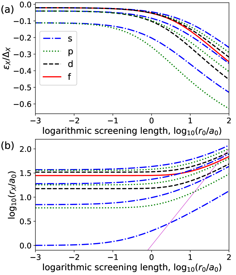
Figure 1: Screening length dependence of (a) exciton energy levels and (b) exciton radii for the case of $\sigma=1$. The exciton energies are normalized with respect to the exciton binding energy, $\Delta_{\text{X}}$. The dash-dot lines are exciton energy levels with $l=0$ and $n=2,3,4$ ($2s$, $3s$, $4s$ excitons) for (a) and $n=1,2,3,4$ ($1s$, $2s$, $3s$, $4s$ excitons) for (b) from low to high. The dot lines are levels with $l=1$ and $n=2,3,4$ ($2p$, $3p$, $4p$ excitons). The dash lines are levels with $l=2$ and $n=3,4$ ($3d$, $4d$ excitons). The solid line is the level with $l=3$ and $n=4$ ($4f$ exciton). The thin straight line denotes $r_{\text{X}}=r_{0}$.

Here, energy levels and average radii for the lowest few states of the exciton with $l=0,1,2,3$ are calculated as functions of screening length and the results for mass ratio $\sigma=1$ are shown in Fig. 1. All energies are normalized with respect to the exciton binding energy $\Delta_{X}$. So, the exciton ground-state ($1s$) energy is always at $-\Delta_{X}$ (not shown). The energy levels with $l=0,1,2,3$ ($s,p,d,f$-like) are shown by dash-dot, dotted, dashed, and solid curves, respectively. The results of Fig. 1(a) are essentially the same as those reported in Ref. wu2019exciton, . As $r_{0}\rightarrow 0$, the Rytova-Keldysh potential reduces to the Coulomb potential in 2D, and we can benchmark the exciton energy levels calculated by our method with the bound-state energy levels of a 2D hydrogen atom. The bound-state energy levels of a 2D hydrogen atom are given by the analytic formulayang1991analytic

$$\varepsilon_{\text{X},n}/\varepsilon_{0}=-\frac{1}{2\left(n-{1}/{2}\right)^{2}}\frac{1}{\sigma+1}.$$ (21)

For $\sigma=1$, the first four energy levels are $\varepsilon_{\text{H}}=-1$, $-1/9$, $-1/25$, $-1/49$, respectively. As can be seen in Fig. 1(a), the spectrum of the 2D hydrogen atom is successfully reproduced as $r_{0}\rightarrow{0}$. In the other limit ($r_{0}/a_{0}\gg{1}$), the exciton spectrum becomes quite different. The degenerate levels for each principle number are split into multiple energy levels for different angular momenta. This is because the dynamical symmetry generated by the Runge-Lenz vector is broken in the non-Coulombic potential for finite $r_{0}$. Note that in the group of energy levels with the same principle number the level with higher absolute value of angular momentum lies lower. For $r_{0}/a_{0}=100$, the $2p$ exciton has the binding energy $~{}60$ % of $1s$ exciton, which is in sharp contrast to the case of $r_{0}/a_{0}\rightarrow{0}$ where the binding energy of $2p$ exciton is only about $11$ % of the binding energy of $1s$ exciton.

In Fig. 1(b), the screening length dependence of the exciton radius is shown. The exciton radius is defined by

$$r_{\text{X},i} \equiv \frac{\int\Psi^{*}_{\text{X},i}(\mathbf{r})r\Psi_{\text{X},i}(\mathbf{r})\text{d}^{2}r}{\int\Psi^{*}_{\text{X},i}(\mathbf{r})\Psi_{\text{X},i}(\mathbf{r})\text{d}^{2}r}.$$ (22)

For the zero screening-length limit, it can be verified that the calculated exciton radius is consistent with the analytical formyang1991analytic

$$r_{\text{X},(n,l)}/a_{0}=\frac{\sigma+1}{2}\left[3n(n-1)-|l|^{2}+1\right]$$ (23)

with $\sigma=1$. As the screening length increases, the exciton radius also gradually increases with a slope smaller than that for the screening length. Eventually, the screening length exceeds exciton radius for most excitons considered. A thin straight line for $r_{\text{X}}=r_{0}$ is plotted in the figure to indicate the point of crossing for $r_{\text{X}}$ and $r_{0}$. In the regime where exciton radii are shorter than the screening length, the electron-hole attractive interaction becomes very different from the Coulomb interaction but closer to a logarithmic interaction as mentioned in Sec. II.1. This is consistent with the finding in the screening length dependence of exciton energy levels in Fig. 1 (a).

III.2 Trion energy levels

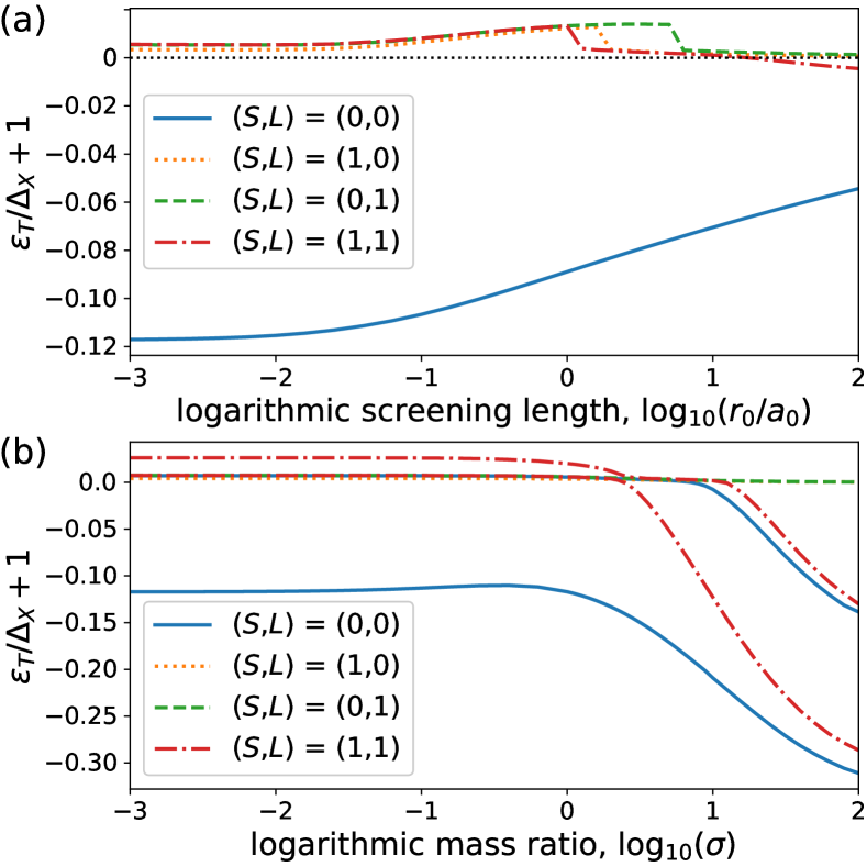
Figure 2: (a) screening length dependence of trion energy levels with $\sigma=1$ and $\kappa=1$; (b) mass ratio dependence of trion energy levels with $r_{0}=0$ and $\kappa=1$. The vertical axis gives the energy difference between the trion and the $1s$ exciton in a fraction of the exciton binding energy ($\Delta_{\text{X}}=|\varepsilon_{\text{X},(n,l)=(1,0)}|$). For $(S,L)=(0,0)$ and $(S,L)=(1,1)$, the dependence of the two lowest-energy (principle number $N=1$ and $N=2$) trion energy levels is listed.

Here, we calculate the energy levels ($\varepsilon_{\text{T}}$) of low-lying trion states by varying the mass ratio ($\sigma$) and screening length ($r_{0}$), and the results are shown in Fig. 2. While only negative trions are considered explicitly, the binding energy of positive trions can be obtained by reversing the mass ratio ($\sigma\rightarrow 1/\sigma$). It is found that, the symmetric ($S=0$) trion with zero angular momentum ($L=0$) is bound for all the parameter regimes considered. The trion binding energy ($\Delta_{\text{T}}=\varepsilon_{\text{X},{1s}}-\varepsilon_{\text{T}}$) at $r_{0}=0$ and $\sigma=1$ is about $12.0$% of the exciton binding energy ($\Delta_{\text{X}}=|\varepsilon_{\text{X},{1s}}|$), which is only slightly smaller than the highest reported value $12.1$% calculated by the stochastic variational methodusukura1999stability . The trion binding energy at $r_{0}=0$ and $\sigma=0$ is about $11.93$% of the exciton binding energy, which is also slightly smaller than the reported value $12.0$%usukura1999stability . The small discrepancy could come from the restriction of the present variational trion wavefunction, whose asymptote behavior is only described by a few exponential functions, while the stochastic variational method uses hundreds of Gaussian basis functions to describe its asymptote behavior.

In addition to the trion with $(S,L)=(0,0)$, we also considered the lowest energy levels of other sets of quantum numbers for $(S,L)$. We note that due to symmetry the trion with angular quantum number $L=-1$ is degenerate with the trion with $L=1$ and the same permutation index. So, we only present results for the antisymmetric ($S=1$) negative trion with $L=1$. It was found the negative trion with $(S,L)=(1,1)$ is bound for $\sigma>3$ (or $\sigma<0.34$ for the positive trion) in several literaturessergeev2001singlet ; sergeev2001triplet ; courtade2017charged . As can be seen in Fig. 2 (b), we also find the negative trion is bound for $\sigma>2.6$ in the present calculation. For an even larger $\sigma$, there could exist two bound states for both symmetric and antisymmetric negative trions. Additionally, as shown in Fig. 2 (a), we find that the trion with $(S,L)=(1,1)$ could also be bound for $\sigma=1$ and a large screening length ($r_{0}/a_{0}>20$). These results suggest that stable antisymmetric negative trions can exist for large electron-hole mass ratios or long screening lengths. On the other hand, for trions with quantum numbers $(S,L)=(0,{1})$ and $(S,L)=(1,0)$, we do not find any bound state in the present parameter range.

III.3 Excitons and trions in TMDCs

Table 1: Trion binding energies of TMDCs

Materials	$m_{\text{e}}/m_{0}$	$m_{\text{h}}/m_{0}$	$r_{0}$(Å)	$\kappa$	$\Delta_{\text{X}}$(meV)	$\Delta_{\text{T}^{-}}$(meV)	$\Delta_{\text{T}^{+}}$(meV)	$\Delta^{\star}_{\text{T}^{-}}$(meV)	$\Delta^{\star}_{\text{T}^{+}}$(meV)
$\text{MoS}_{2}$	$0.47$	$0.54$	$44.68$	$1.0$	526.0 ($526.5$)	31.6 ($32.0$)	31.6 ($31.6$)	0.4	2.4
				$2.0$	348.4 ($348.6$)	24.4 ($24.7$)	24.5 —–	–	–
$\text{MoSe}_{2}$	$0.55$	$0.59$	$53.16$	$1.0$	476.7 ($476.9$)	27.7 ($27.7$)	27.6 ($27.8$)	1.0	2.0
				$2.0$	323.1 ($322.9$)	21.9 ($22.1$)	21.9 —–	–	–
$\text{WS}_{2}$	$0.32$	$0.35$	$40.17$	$1.0$	508.6 ($509.8$)	32.4 ($33.1$)	32.4 ($33.5$)	0.0	1.1
				$2.0$	322.4 ($322.9$)	23.8 ($24.3$)	23.9 —–	–	–
$\text{WSe}_{2}$	$0.34$	$0.36$	$47.57$	$1.0$	456.0 ($456.4$)	28.3 ($28.5$)	28.3 ($28.5$)	0.4	1.1
				$2.0$	294.6 ($294.6$)	21.3 ($21.5$)	21.3 —–	–	–
$\text{WSe}_{2}/BN(D^{0})$	$0.46$	$0.43$	$46.8$	$4.0$	186.0 [$186.0$]	13.2 [$15.2$]	13.2 [$13.7$]	–	–
$\text{WSe}_{2}/BN(A^{0})$	$0.38$	$0.43$	$46.8$	$4.0$	172.0 [$171.8$]	23.0 [$29.0$]	19.0 [$21.0$]	–	–

We then apply the present method to calculate trion binding energies of 2D materials. Since the EHX effect is quite significant in TMDCs, we have considered the effect of EHX in monolayer WSe₂ as an example. The strengths of EHX $U^{x}_{\tau}$ in a contact potential approximation for the intravalley exciton ($A^{0}$) and intervalley exciton ($I^{0}$) have been calculated via density-functional theory (DFT) in Ref. YCPRL, . The $U^{x}_{\tau}$ values obtained for $A^{0}$ and $I^{0}$ are $4.17$ $\text{eV/\AA}^{2}$ for $\tau=1$ and $4.80$ $\text{eV/\AA}^{2}$ for $\tau=2$, respectively. For comparison purpose, we first list the calculated exciton and trion binding energies obtained by the present method with $U^{x}_{\tau}$ set to zero. The results for binding energies of exciton ($\Delta_{X}$), negative trion ($\Delta_{T^{-}}$), and positive trion ($\Delta_{T^{+}}$) with $(S,L)=(0,{0})$ are listed in the sixth, seventh and eighth columns in Table 1, respectively. The numbers in parentheses under these three columns are corresponding results obtained previously by using the path-integral Monte Carlo methodkylanpaa2015binding . The binding energies of excited states of negative trions ($\Delta_{T^{-}}^{*}$) and positive trions ($\Delta_{T^{+}}^{*}$) with $(S,L)=(1,1)$ are also shown in the ninth and tenth columns of Table 1. As shown in the Table, the difference between the present calculation and the path-integral Monte Carlo calculation is fairly small ($<0.2$%). The main resource of the discrepancy is attributed to the small number of basis functions used in the present variational wavefunctions, but a smaller part of the discrepancy might also come from the statistical fluctuation of the Monte Carlo method.

We then include the EHX interaction with suitable values of $U^{x}_{\tau}$ for simulating WSe₂ encapsulated by boron-nitride (BN) and calculate the exciton and trion binding energies. The results are presented in the last row of Table 1. For the case of BN-encapsulated monolayer WSe₂, accurate exciton and trion binding energies have been measured experimentallyliu2019magnetophotoluminescence ; liu2019gate , the binding energies of trions with different valley combinations deduced from the experimental observation are also listed (inside square brackets) in the last row of Table 1. The parameters used for the present calculations are obtained from Ref. liu2019magnetophotoluminescence, , but slightly modified to take into account the correction due to the EHX interaction. With the modified parameters and an extension of basis functions to improve convergence, the energy levels of the exciton Rydberg series for $1s$, $2s$, $3s$, and $4s$, respectively are $-172.0$, $-43.7$, $-19.4$, and $-10.6$ meV with respect to the band gap. The results are in very good agreement with the experimentliu2019magnetophotoluminescence . For the positive trion (T⁺) associated with the bright exciton (A⁰) we adopted $U^{x}_{1}=4.17\text{ eV/\AA}^{2}$YCPRL and $U^{x}_{2}=0$, since the second hole is in $K^{\prime}$ valley with opposite spin. For both positive trion (T⁺) and negative trion (T^-) associated with the dark exciton (D⁰) we adopted $U^{x}_{1}=0$YCPRL and $U^{x}_{2}=4.8\text{ eV/\AA}^{2}$YCPRL , since the second electron (hole) in $K^{\prime}$ valley has the same spin as the counterpart particle in $K$ valley. For the negative dark trion (D^-), the binding energy is calculated to be $13.2$ meV, while for trion associated with bright exciton (A⁰), the calculated trion binding increases to $19.0$ meV for the positive trion (A⁺) and to $23.0$meV for the negative trion (A^-). The difference is caused by the effect of EHX interaction. For the positive dark trion (D⁺), there is an intervalley EHX interaction between the second hole and the electron, which leads to a reduction in trion binding. For the positive bright trion (A⁺), the EHX interaction exists between the first hole and the electron, which gives a reduction in binding energy of the bright exciton (A⁰), while the there is no EHX interaction between the second hole and the electron, thus the trion binding becomes enhanced. Similar scenario exists for the negatively charged bright exciton (A^-) which consists of a bight exciton (A⁰) in the K valley and another electron in the lower conduction band in the same valley in our consideration. As shown in Table 1, there is reasonably good agreement between calculated results and experimental observations for most cases. Note that the energy level of the negative bright trion (A^-) observed experimentallyliu2019magnetophotoluminescence is red shifted and split by the Coulomb exchange between the intravalley trion and the intervalley trioncourtade2017charged . The trion binding calculated in the present model is significantly smaller than the observed values of $29$ meV ($35$ meV) for the $A_{1}^{-}$ ($A_{2}^{-}$) peak observed in monolayer WSe$2$. To make a more meaningful comparison between the theory and experiment, we also need to consider the intervalley exchange interaction between the electron in the upper conduction band at the K valley and the electron in the lower conduction band at the K’ vally for the intervalley trion. Furthermore, there may be electron traps in the sample that can lead to localized negative trions and enhance their binding energy. These effects will be considered in future work.

Based on the present calculation, weakly-bound excited-state trions with quantum numbers $(S,L)=(1,{1})$ for positive trions of MoS₂, MoSe₂, WS₂, WSe₂ and for negative trions of above TMDCs except for WS₂ are found. However, these excited-state trions have not been clearly identified experimentally yet. One of the reasons could be that the binding energies of these excited-state trions are so small that the trion transition peaks are difficult to be distinguished from the exciton transition peaks in optical spectra. The present model might also be too simple to describe excited-state trions in realistic 2D materials, since Berry-curvature effecthichri2019charged , Coulomb exchange between charge carrierscourtade2017charged , and valley degrees of freedomdurnev2018excitons have been neglected. It is uncertain that these excited-state trions can still be stable in an improved model. It is a question we seek to answer in the future.

IV Conclusion

By using 2D STOs as basis functions and variational techniques, exciton and trion energy levels can be solved efficiently with fairly accurate results. Ground-state and excited-state trions are studied by the present method. The trion wavefunction and eigenenergy are indicated by a permutation index ($S$) and an angular momentum ($L$). We find that a weakly-bound excited-state of the negative trion with quantum numbers $(S,L)=(1,{1})$ could exist with a large electron-hole mass ratio ($\sigma>2.6$) or a long screening length ($r_{0}/a_{0}>20$). The present method is also implemented to study trion binding energies of TMDCs. The calculated binding energy of the ground-state trion is well matched with another calculation in literature by using path-integral Monte Carlo method. Present calculations also suggest possible existence of weakly-bound excited-state trions with $(S,L)=(1,{1})$ for both negative and positive trions of MoS₂, MoSe₂, WSe₂ and the positive trion of WS₂ if the dielectric screening constant is sufficiently small. By including the EHX interaction in the calculation of exciton and trion binding energies in monolayer WSe₂ for various electronic configurations, we find that the calculated exciton and trion binding energies agree well with the experimentally observed values.

Appendix A Variationally optimized orbital method

A.1 Hamiltonians in effective atomic unit

The exciton and trion Hamiltonians can be written by the forms

$$\mathcal{H}_{\text{X}}(\mathbf{r}) = -\frac{\sigma+1}{2}\nabla^{2}-V(r),$$ (24)

$$\mathcal{H}_{\text{T}}(\mathbf{r}_{1},\mathbf{r}_{2}) = \mathcal{H}_{\text{X}}(\mathbf{r}_{1})+\mathcal{H}_{\text{X}}(\mathbf{r}_{2})-\sigma\bm{\nabla}_{1}\cdot\bm{\nabla}_{2}+V(r_{12}),$$

where $\sigma=m_{\text{e}}/m_{\text{h}}$. The two Hamiltonians are expressed with length unit in ”$a_{0}$” (effective Bohr radius) and energy unit in ”$\varepsilon_{0}$” (effective Hartree), which are given by $a_{0}=\kappa a_{\text{B}}{m_{0}}/{m_{\text{e}}}$ and $\varepsilon_{0}=(2\text{Ry}/\kappa^{2})m_{\text{e}}/{m_{0}}$, where $m_{0}$ is the free electron mass, $a_{\text{B}}\simeq 0.52918$ Å  ( the Bohr radius ) and $\text{Ry}\simeq 13.606$ eV (the Rydberg). The Rytova-Keldysh potential becomes

$$V(r) = \int\;e^{\mathtt{i}\mathbf{k}\cdot\mathbf{r}}\left[\frac{2\pi}{|\mathbf{k}|\left(1+|\mathbf{k}|\rho_{0}\right)}\right]\frac{\text{d}^{2}k}{(2\pi)^{2}},$$ (26)

with $\rho_{0}=r_{0}/\kappa$.

A.2 Matrix formulations and matrix elements

Given the basis-function set, we still need to solve the expansion coefficients for wavefunctions. Based on the variational principle, the expansion coefficients ($u_{a,i}$) for exciton states in Eq. (16) and the exciton eigenenergies ($\varepsilon_{\text{X},i}$) can be solved from the eigenvalue equation

$$\sum_{b}h_{ab,\tau}u_{b,i}=\varepsilon_{\text{X},i}\sum_{b}o_{ab}u_{b,i},$$ (27)

where $h_{ab,\tau}=t_{ab}+v_{ab}+x_{ab,\tau}$ is the the exciton Hamiltonian matrix with $t_{ab}=-[(\sigma+1)/2]\int\phi^{*}_{a}(\mathbf{r})\nabla^{2}\phi_{b}(\mathbf{r})\text{d}^{2}{r}$, the kinetic integral, $v_{ab}=-\int\phi^{*}_{a}(\mathbf{r})V(r)\phi_{b}(\mathbf{r})\text{d}^{2}r$, the potential integral, and $x_{ab,\tau}=[U^{x}_{\tau}/(2\pi)]\delta_{n_{a},1}\delta_{ab}$ is the exchange integral. $o_{ab}=\int\phi^{*}_{a}(\mathbf{r})\phi_{b}(\mathbf{r})\text{d}^{2}r$ is the overlap integral.

Similarly, the expansion coefficients ($C_{ab,I}$) for trion states in Eq. (17) and the trion eigenenergies ($\varepsilon_{\text{T},I}$) can be solved from the eigenvalue equation

$$\sum_{cd}H_{ab,cd}C_{cd,I}=\varepsilon_{\text{T},I}\sum_{cd}O_{ab,cd}C_{cd,I},$$ (28)

where $H_{ab,cd}$ is the trion Hamiltonian matrix and $O_{ab,cd}$ is the trion overlap matrix. For the two electrons being identical particles, the quantum numbers of a trion is $I=(N,S,L)$, and the trion Hamiltonian matrix and the overlap matrix are written as

$$H_{ab,cd} = h_{ac,\tau}o_{bd}+o_{ac}h_{bd,\tau}+X_{ab,cd}+\bar{V}_{ab,cd}$$

$$+(-1)^{S}(h_{ad,\tau}o_{bc}+o_{ad}h_{bc,\tau}+X_{ab,dc}+\bar{V}_{ab,dc}),$$

and $O_{ab,cd}=o_{ac}o_{bd}+(-1)^{S}o_{ad}o_{bc}$, with

$$X_{ab,cd} = -\sigma\int\phi^{*}_{a}(\mathbf{r}_{1})\phi^{*}_{b}(\mathbf{r}_{2})$$

$$\times\bm{\nabla}_{1}\cdot\bm{\nabla}_{2}\left[\phi_{c}(\mathbf{r}_{1})\phi_{d}(\mathbf{r}_{2})\right]\text{d}^{2}r_{1}\text{d}^{2}r_{2}$$

being called the ”kinetic-polarization” integral and

$$\bar{V}_{ab,cd} = \int\phi^{*}_{a}(\mathbf{r}_{1})\phi^{*}_{b}(\mathbf{r}_{2})V(r_{12})\phi_{c}(\mathbf{r}_{1})\phi_{d}(\mathbf{r}_{2})\text{d}^{2}r_{1}\text{d}^{2}r_{2}$$

the two-particle mutual-interaction integral. On the other hand, for the case that the two electrons reside at different valleys, the trion Hamiltonian matrix should be rewritten as

$$H_{ab,cd} = h^{(1)}_{ac,\tau_{1}}o_{bd}+o_{ac}h^{(2)}_{bd,\tau_{2}}+X_{ab,cd}+\bar{V}_{ab,cd},$$

and the overlap matrix becomes $O_{ab,cd}=o_{ac}o_{bd}$, while the quantum numbers are given by $I=(N,L)$. Here $h^{(1)}$ and $h^{(2)}$ can be different since the effective masses of the two electrons in the trion in TMDCs can be in different conduction bands due to the presence of two closely-spaced conduction bands in K (K’) valley.

A.3 Orbital integrals

By using the STOs, analytic expressions for calculating orbital integrals can be derived. The overlap integral is given by

$$o_{ab} = \delta_{l_{a},l_{b}}\frac{(n_{a}+n_{b}-1)!}{(\zeta_{a}+\zeta_{b})^{n_{a}+n_{b}}},$$ (29)

and the kinetic integral is found as

$$t_{ab} = -\frac{\delta_{l_{a},l_{b}}(\sigma+1)}{2}\frac{(n_{a}+n_{b}-1)!}{\left(\zeta_{a}+\zeta_{b}\right)^{n_{a}+n_{b}}}$$ (30)

$$\times\Bigg{\{}(1-\delta_{n_{b},1})\frac{\left[(n_{b}-1)^{2}-l_{b}^{2}\right]\left(\zeta_{a}+\zeta_{b}\right)^{2}}{(n_{a}+n_{b}-1)(n_{a}+n_{b}-2)}$$

$$-\frac{\left[(2n_{b}-1)\zeta_{b}\right]\left(\zeta_{a}+\zeta_{b}\right)}{(n_{a}+n_{b}-1)}+\zeta^{2}_{b}\Bigg{\}}.$$

By using the cross-differential operator in polar coordinates

$$\bm{\nabla}_{1}\cdot\bm{\nabla}_{2} = \cos\left(\varphi_{1}-\varphi_{2}\right)\left(\frac{\partial}{\partial{r}_{1}}\frac{\partial}{\partial{r}_{2}}+\frac{1}{r_{1}}\frac{\partial}{\partial{\varphi}_{1}}\frac{1}{r_{2}}\frac{\partial}{\partial{\varphi}_{2}}\right)$$

$$-\sin\left(\varphi_{1}-\varphi_{2}\right)\left(\frac{1}{r_{1}}\frac{\partial}{\partial{\varphi}_{1}}\frac{\partial}{\partial{r}_{2}}-\frac{1}{r_{2}}\frac{\partial}{\partial{\varphi}_{2}}\frac{\partial}{\partial{r}_{1}}\right),$$

the kinetic-polarization integral is give by

$$X_{ab,cd} = -\frac{\sigma}{2}\frac{(n_{a}+n_{c}-2)!}{(\zeta_{a}+\zeta_{c})^{n_{a}+n_{c}-1}}\frac{(n_{b}+n_{d}-2)!}{(\zeta_{b}+\zeta_{d})^{n_{b}+n_{d}-1}}$$ (31)

$$\times\Big{[}\big{(}\delta_{l_{c},l_{a}-1}\delta_{l_{d},l_{b}+1}+\delta_{l_{c},l_{a}+1}\delta_{l_{d},l_{b}-1}\big{)}$$

$$\times\left(g_{ac}g_{bd}-l_{c}l_{d}\right)+\big{(}\delta_{l_{c},l_{a}-1}\delta_{l_{d},l_{b}+1}$$

$$-\delta_{l_{c},l_{a}+1}\delta_{l_{d},l_{b}-1}\big{)}\left(l_{d}g_{ac}-l_{c}g_{bd}\right)\Big{]},$$

with $g_{ac}=n_{c}-1-{\zeta_{c}(n_{a}+n_{c}-1)}/{(\zeta_{a}+\zeta_{c})}$.

For the potential integral and the two-particle mutual-iteraction integral, analytical solutions are difficult to derive. Formulas for numerical computation are more feasible. The potential integral can be rewritten as

$$v_{ab} = -\int{p}_{ab}(\mathbf{r})V(r)\text{d}^{2}r=-\int\tilde{{p}}_{ab}(\mathbf{k})\tilde{V}(k)\frac{\text{d}^{2}k}{(2\pi)^{2}},$$

where ${p}_{ab}(\mathbf{r})=\phi^{*}_{a}(\mathbf{r})\phi_{b}(\mathbf{r})$ is a density matrix function with Fourier transform given by $\tilde{{p}}_{ab}(\mathbf{k})=\int{p}_{ab}(\mathbf{r})e^{-\mathtt{i}\mathbf{k}\cdot\mathbf{r}}\text{d}^{2}r$ , and $\tilde{V}({k})=\int V(\mathbf{r})e^{-\mathtt{i}\mathbf{k}\cdot\mathbf{r}}\text{d}^{2}r={2\pi}/[k({1+kr_{*}})]$ is the Fourier transform of the Rytova-Keldysh potential. Since the density matrix function is also a STO, the Fourier transform can be solved by using Eq. (LABEL:Rk_formula). We have

$$\tilde{p}_{ab}(\mathbf{k}) = \frac{e^{\mathtt{i}(l_{b}-l_{a})\varphi_{\mathbf{k}}}}{2\pi}\tilde{\mathcal{R}}_{n_{a}+n_{b}-1,l_{b}-l_{a}}(\zeta_{a}+\zeta_{b},k),$$ (32)

where $\tilde{\mathcal{R}}_{n_{a}+n_{b}-1,l_{b}-l_{a}}(2\zeta,k)$ is given by Eq. (LABEL:Rk_formula). The potential integral becomes

$$v_{ab} = \frac{-\delta_{l_{a},l_{b}}}{(2\pi)^{2}}\int^{\infty}_{0}\tilde{\mathcal{R}}_{n_{a}+n_{b}-1,0}(\zeta_{a}+\zeta_{b},k)\tilde{V}(k)k\text{d}k.$$

The integral in Eq. (LABEL:potential_integral) can be computed numerically. Note that even though the potential integral in real space can have analytical solution, the infinite summations from the Bessel function and the Struve function still consume computational resource. Besides, numerical integration over one-variable function is not so demanding. The two-particle mutual-interaction integral can also be written in terms of density matrix functions, as

$$\bar{V}_{ab,cd} = \int{p}^{*}_{ca}(\mathbf{r}_{1})V(r_{12}){p}_{bd}(\mathbf{r}_{2})\text{d}^{2}r_{1}\text{d}^{2}r_{2}$$ (34)

$$= \frac{1}{(2\pi)^{2}}\int\tilde{{p}}^{*}_{ca}(\mathbf{k})\tilde{V}(k)\tilde{{p}}_{bd}(\mathbf{k})\text{d}^{2}k.$$

By using Eq. (32) and Eq. (LABEL:Rk_formula), the above equation becomes

$$\bar{V}_{ab,cd} = \frac{\delta_{l_{a}-l_{c},l_{d}-l_{b}}}{(2\pi)^{3}}\int^{\infty}_{0}\tilde{\mathcal{R}}^{*}_{n_{a}+n_{c}-1,\Delta{l}}(\zeta_{a}+\zeta_{c},k)$$ (35)

$$\times\tilde{\mathcal{R}}_{n_{b}+n_{d}-1,\Delta{l}}(\zeta_{b}+\zeta_{d},k)\tilde{V}(k)k\text{d}k,$$

with $\Delta{l}=l_{a}-l_{c}=l_{d}-l_{b}$. Therefore, the two-particle mutual-integral is reduced to an one-variable integral, which can be computed efficiently via gaussian-quadrature integration.

A.4 Numerical procedure

Both the exciton eigenenergy $\varepsilon_{\text{X},i}$ and the trion eigenenergy $\varepsilon_{\text{T},I}$ are depended on the shielding constant $\zeta$ of STOs. Therefore, by varying $\zeta$ to minimize each eigenenergy of the exciton or trion Hamiltonian, an optimized exponential function can be found for each STO. However, if all shielding constants and linear variational parameters are varied, the optimization problem could be overdetermined and thus multiple local minimums would be found. It will result slow convergence or oscillations in the optimization process. The calculation procedure should be designed properly to avoid this problem.

Our procedure for an exciton calculation is given as follows. For the first step of an exciton calculation, for each angular momentum $l$ we use $n_{l}$ STOs with $n_{l}$ different principal quantum numbers to construct an exciton wavefunction and optimize one shielding constant for each eigenstate. Subsequently, we will have $n_{l}$ eigenstates and $n_{l}$ optimized shielding constants for each eigenenergy. Then, we use these $n_{l}$ STOs with different shielding constants as basis functions to construct the Hamiltonian matrix given in in Eq. (27) and solve $n_{l}$ lowest eigenvalues and eigenfunctions from the equation. The $n_{l}$ lowest eigenstates can be assigned as the $n_{l}$ lowest-lying exciton states for the specific angular momentum $l$. Note that these $n_{l}$ wavefunctions of lowest $n_{l}$ excitons are orthogonal mutually. To improve the binding energy, one may add a few STOs with the same $n_{l}$ but different shielding constants, $\zeta_{i}$ by choosing $\zeta_{i}$ to be the optimized shielding constant $\zeta_{n_{l}}$ multiplied by a suitable scaling factor to form an even-tempered serieschang2018crossover . These additional STOs will be needed especially for getting a convergent result for the $1s$ state when the EHX interaction is included.

The procedure for a trion calculation is similar. Each trion configuration $(1/\sqrt{2})[\phi_{a}(\mathbf{r}_{1})\phi_{b}(\mathbf{r_{2}})+(-1)^{S}\phi_{a}(\mathbf{r}_{2})\phi_{b}(\mathbf{r_{1}})]$ can be indicated by $(S,a,b)$ with $a=(n_{a},l_{a},\zeta_{a})$ and $b=(n_{b},l_{b},\zeta_{b})$. The indices are restricted by $l_{a}+l_{b}=L$ with $i_{a}\leq{i_{b}}$ for $S=0$, and $i_{a}<i_{b}$ for $S=1$. For the first step of a trion calculation, we calculate $\mathcal{N}$ eigenenergies for each state with quantum numbers $(S,L)$ by optimizing the shielding constant $\zeta=\zeta_{a}=\zeta_{b}$ for each state. We subsequently use all configurations with $\zeta_{a}$, $\zeta_{b}$ being given by $\mathcal{N}$ different shielding constants to construct the variational trion wavefunction. Finally, we use the variational trion wavefunction to derive the trion eigenvalue equation as in Eq. (28), and then solve $\mathcal{N}$ lowest eigenvalues and eigenfunctions from the equation. The $\mathcal{N}$ lowest eigenvalues and eigenfunctions can be assigned as the $\mathcal{N}$ lowest trion eigenenergies and wavefunctions.

In our calculations, STOs with principal quantum numbers ($|l|+1\leq{n}\leq 6$) and angular momentum $|l|\leq 5$ are included to the basis set. For an exciton calculation with the angular momentum $l$, there are $n_{l}=6-|l|$ shielding constants solved from optimizing single-zeta exciton wavefunctions, and $n_{l}$ excitons can be found. For a trion calculation, at least two shielding constants of the same $n_{l}$ are used to solve the optimized trion wavefunctions. When the EHX term is included, we added more ($~{}10$) STOs basis functions for $n_{l}=1$ in order to get convergent result.

References

- (1) K. Kheng, R. T. Cox, M. Y. d’Aubigné, F. Bassani, K. Saminadayar, and S. Tatarenko, Phys. Rev. Lett., 71, 1752 (1993).
- (2) V. Huard, R. T. Cox, K. Saminadayar, A. Arnoult, and S. Tatarenko, Phys. Rev. Lett., 84, 187 (2000).
- (3) K. F. Mak, K. He, C. Lee, and G. H. Lee, J. Hone, T. F. Heinz, and J. Shan, Nature materials, 12, 207 (2013).
- (4) Y. Lin, X. Ling, L. Yu, S. Huang, A. L. Hsu?? Y. H. Lee, J. Kong, M. S. Dresselhaus, T. Palacios, Nano Lett. 14, 5569 (2014)
- (5) T. C. Berkelbach, M. S. Hybertsen, and D. R. Reichman, Phys. Rev. B, 88, 045318 (2013).
- (6) T. C. Berkelbach, and D. R. Reichman, Ann. Rev. Condens. Matter Phys., 9, 379 (2018).
- (7) M. V. Durnev and M. M. Glazov, Physics-Uspekhi, 61, 825 (2018).
- (8) A. Esser, E. Runge, R. Zimmermann, and W. Langbein, Phys. Rev. B, 62, 8232 (2000).
- (9) M. Drüppel, T. Deilmann, P. Krüger, and M. Rohlfing, Nat. Commun., 8, 2117 (2017).
- (10) A. Torche and G. Bester, Phys. Rev. B, 100, 201403(R) (2019).
- (11) R. Tempelaar and T. C. Berkelbach, Nat. Commun., 10, 3419 (2019).
- (12) Y. V. Zhumagulov, A. Vagov, N. Yu. Senkevich, D. R. Gulevich, and V. Perebeinos, Phys. Rev. B, 101, 245433 (2020).
- (13) Y. V. Zhumagulov, A. Vagov, D. R. Gulevich, P. E. Faria Jr., and V. Perebeinos, J. Chem. Phys., 153, 044132 (2020).
- (14) M. Z. Mayers, T. C. Berkelbach, M. S. Hybertsen, and D. R. Reichman, Phys. Rev. B, 92, 161404(R) (2015).
- (15) I. Kylänpää and H.-P. Komsa, Phys. Rev. B, 92, 205418 (2015).
- (16) K. A. Velizhanin and A. Saxena, Phys. Rev. B, 92, 195305 (2015).
- (17) M. Szyniszewski, E. Mostaani, N. D. Drummond, and V. I. Fal’ko, Phys. Rev. B, 95, 081301(R) (2017).
- (18) E. Mostaani, M. Szyniszewski, C. H. Price, R. Maezono, M. Danovich, R. J. Hunt, N. D. Drummond, and V. I. Fal’ko, Phys. Rev. B, 96, 075431 (2017).
- (19) D. E. Phelps and K. K. Bajaj, Phys. Rev. B, 27, 4883 (1983).
- (20) B. Stébé and A. Ainane, Superlattices and microstructures, 5, 545 (1989).
- (21) J. Usukura, and Y. Suzuki, and K. Varga, Phys. Rev. B, 59, 5652 (1999).
- (22) W. Y. Ruan, K. S. Chan, and E. Y. B. Pun, J. Phys.: Condens. Matter, 12, 7905 (2000).
- (23) P. Redliński, and J. Kossut, Solid State Commun., 118, 295 (2001).
- (24) L. Hilico, B. Greḿaud, T. Jonckheere, N. Billy, and D. Delande, Phys. Rev. B 66, 022101 (2002).
- (25) D. W. Kidd, D. K. Zhang, and K. Varga, Phys. Rev. B, 93, 125423 (2016).
- (26) M. Van der Donck, M. Zarenia, and F. M. Peeters, Phys. Rev. B, 96, 035131 (2017).
- (27) A. Hichri, I. Ben Amara, S. Ayari, and S. Jaziri, J. Phys.: Condens. Matter, 29, 435305 (2017).
- (28) R. Y. Kezerashvili and S. M. Tsiklauri, Few-Body Systems, 58, 18 (2017).
- (29) M. Van der Donck, M. Zarenia, and F. M. Peeters, Phys. Rev. B, 97, 195408 (2018).
- (30) I. Filikhin, R. Y. Kezerashvili, S. M. Tsiklauri and B. Vlahovic, Nanotechnology, 29, 124002 (2018).
- (31) A. Hichri, S. Jaziri, and M. O. Goerbig, Phys. Rev. B, 100, 115426 (2019).
- (32) J. Yan and K. Varga, 101, 235435 (2020).
- (33) N. S. Rytova, Vestn. Mosk. Univ. Fiz. Astron., 3, 30 (1967).
- (34) L. V. Keldysh, J. Exp. Theoret. Phys. Lett., 29, 658 (1979).
- (35) T. Kato, Commun. Pure Appl. Math., 10, 151 (1957).
- (36) T. C. Scott, A. Lüchow, D. Bressanini, and J. D. Morgan III, Phys. Rev. A, 75, 060101(R) (2007).
- (37) C. Zener, Phys. Rev., 36, 51 (1930).
- (38) I. N. Levine, D. H. Busch, and H. Shull, Quantum chemistry (Pearson Prentice Hall Upper Saddle River, NJ, 6th edition, 2009).
- (39) S. Wu, L. Cheng, and Q. Wang, Phys. Rev. B, 100, 115430 (2019).
- (40) J. C. G. Henriques and N. M. R. Peres, Phys. Rev. B, 101, 035406 (2020).
- (41) M. F. C. Martins Quintela and N. M. R. Peres, The European Physical Journal B, 93, 1 (2020).
- (42) Y.-C. Chang, S.-Y. Shiau, and M. Combescot, Phys. Rev. B, 98, 235203 (2018).
- (43) M. Rohlfing and S. G. Louie, Phys. Rev. B, 62, 4927 (2000).
- (44) W. Ritz, Journal für die Reine und Angewandte Mathematik, 135, 1 (1909).
- (45) J. K. MacDonald, Phys. Rev. 43 830 (1933)
- (46) E. Liu, J. van Baren, C.-T. Liang, T. Taniguchi, K. Watanabe, N. M. Gabor, Y.-C. Chang, C. H. Lui, Phys. Rev. Lett., 124, 1976802 (2020).
- (47) R. A. Sergeev and R. A. Suris, Nanotechnology, 12, 597 (2001).
- (48) R. A. Sergeev and R. A. Suris, phys. stat. sol. (b), 227, 387 (2001).
- (49) E. Courtade, M. Semina, M. Manca, M. M. Glazov, C. Robert, F. Cadiz, G. Wang, T. Taniguchi, K. Watanabe, M. Pierre, W. Escoffier, E. L. Ivchenko, P. Renucci, X. Marie, T. Amand, and B. Urbaszek, Phys. Rev. B, 96, 085302 (2017).
- (50) X. L. Yang, S. H. Guo, F. T. Chan, K. W. Wong, and W. Y.Ching, Phys. Rev. A, 43, 1186 (1991).
- (51) E. Liu, J. van Baren, T. Taniguchi, K. Watanabe, Y.-C. Chang, and C. H. Lui, Phys. Rev. B, 99, 205420 (2019).
- (52) E. Liu, J. van Baren, Z. Lu, M. M. Altaiary, T. Taniguchi, K. Watanabe, D. Smirnov, and C. H. Lui, Phys. Rev. Lett., 123, 027401 (2019).