Enabling DER Participation in Frequency Regulation Markets

Abstract

Distributed energy resources (DERs) are playing an increasing role in ancillary services for the bulk grid, particularly in frequency regulation. In this paper, we propose a framework for collections of DERs, combined to form microgrids and controlled by aggregators, to participate in frequency regulation markets. Our approach covers both the identification of bids for the market clearing stage and the mechanisms for the real-time allocation of the regulation signal. The proposed framework is hierarchical, consisting of a top layer and a bottom layer. The top layer consists of the aggregators communicating in a distributed fashion to optimally disaggregate the regulation signal requested by the system operator. The bottom layer consists of the DERs inside each microgrid whose power levels are adjusted so that the tie line power matches the output of the corresponding aggregator in the top layer. The coordination at the top layer requires the knowledge of cost functions, ramp rates and capacity bounds of the aggregators. We develop meaningful abstractions for these quantities respecting the power flow constraints and taking into account the load uncertainties, and propose a provably correct distributed algorithm for optimal disaggregation of regulation signal amongst the microgrids.

I Introduction

Electric power systems require the generation and load to be equal at all times. Any discrepancy between the two leads to the deviation of the frequency from its nominal value. This deviation of the frequency leads to many undesirable scenarios. Based on measurements of the frequency deviation, the system operator computes the automatic generation control (AGC) signal as the feedback frequency control to the power system, which appears as the total active power adjustment. Traditionally, frequency regulation services have been provided by individual energy resources, such as coal generation plants or gas turbines. Recently, there has been a trend towards the integration of more DERs into the system to provide these services while reducing thermal and CO₂ emissions. Such integration leads to higher uncertainty in the bulk grid. At the same time, as most DERs are inertialess, they can be effective for frequency regulation due to their high ramp rates. DERs are limited in size and might not meet the minimum size criteria specified by system operators to participate in the frequency regulation market. To address these challenges, the vision is to integrate groups of DERs through distributed energy resource providers (DERPs), or aggregators, which would act as virtual power plants (VPPs) and would be communicating with the system operator. These aggregators do not necessarily own the DERs, they just coordinate their responses. This architecture, illustrated in Figure 1, has been proposed by the California ISO (CAISO) to offer aggregators of DERs the opportunity to sell into its marketplace [2]. The recent Order No. 2222 [3] by the U.S. Federal Energy Regulatory Commission (FERC) also enables aggregators to participate in the energy markets and requires all Regional Transmission Organizations (RTOs) to revise their tariffs to establish DERs as a category of market participant. Using aggregators not only solves the problem of limited capabilities of DERs but also enables the system operator to interact with much fewer entities. This paper is motivated by the need to address the challenges to carry out the vision described above.

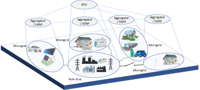
Figure 1: Power system framework. Dashed lines represent communication links and solid lines represent electrical connections. All the microgrids are connected to the bulk grid through the tie lines. The Regional Transmission Organization (RTO) monitors the bulk grid and coordinates with the aggregators, which control the resources inside the microgrids.

Literature Review: Order No. 755 [4] issued by the FERC requires RTOs to compensate energy resources based on the actual frequency regulation provided. The payment to resources comprises of two parts, the capacity and performance payments. The capacity payment compensates resources for their provision of regulation capacity. The performance payment reflects the accuracy of the tracking of the allocated regulation signal. The work [5] describes how different RTOs across the United States have implemented FERC Order 755 for participation of resources in frequency regulation market. In the literature on power networks and smart grid, some works have considered the possibility of obtaining frequency regulation services from collections of homogeneous loads such as electric vehicles (EVs) and thermostatically controlled loads (TCLs), cf. [6, 7, 8]. The work [9] presents a method to model flexible loads as a virtual battery for providing frequency regulation. [10] proposes the use of aggregators to integrate heterogeneous loads such as heat pumps, supermarket refrigerators and batteries present in industrial buildings to provide frequency regulation. The works [11, 12] describe the challenges that need to be overcome for providing frequency regulation by DERs for some European countries. The work [13] provides a framework to emulate virtual power plants (VPPs) via aggregations of DERs and provide regulation services taking into account the power flow constraints. [14] provides a dispatch strategy for an aggregate of ON/OFF devices to provide frequency regulation. In [15, 16, 17], work has been done in the context of microgrids to design mechanisms for optimally allocating a given signal among the DERs within the microgrid. [18] proposes a distributed algorithm to minimize the aggregated cost while satisfying the local constraints and collective demand constraint at the aggregator. However, the aforementioned works assume that the allocated signal from the RTO is available to the aggregator. [19] applies machine learning to forecast the power capacity of VPPs. The work [20] provides a framework for optimal bidding and dispatch of multiple VPPs. [21] proposes the use of renewable energy aggregators to utilize small-scale distributed generators for frequency regulation services via forecasting the available power from individual resources. The work [22] also uses forecasting to estimate the aggregate production from a wind and solar power-based VPP, and then uses the estimation to determine the optimal volume of reserves that can be provided to the system operator. A distributed algorithm for coordinating multiple aggregators to provide frequency regulation, without any consideration of cost, is proposed in [23]. Here, we focus on (i) participation of microgrids in frequency regulation markets operated by the RTO through the identification of appropriate bids and (ii) the coordination among RTO and aggregators to efficiently dis-aggregate the regulation signal amongst the aggregators. The actual tracking performance within the microgrid would depend on the physical condition of the resources. We have provided some results for this in [24] on experiments carried out on the University of California, San Diego (UCSD) microgrid.

Statement of Contributions: We propose a hierarchical framework for the participation of microgrids in the frequency regulation market. We start by briefly reviewing the current practice of frequency regulation from individual resources, consisting of three stages: (i) market clearance, (ii) disaggregation of the regulation signal and (iii) real-time tracking of the regulation signal. Our first contribution is the identification of the limitations of current practice and the challenges that need to be overcome for integration of microgrids. Our second contribution is the identification of abstractions for the capacity, cost of generation, and ramp rates of a microgrid as a combination of the individual energy resources that compose it, along with a formal description of its convexity and monotonicity properties. Building on our preliminary work [1], here we extend our abstractions to the case when the loads inside the microgrid do not remain constant for the regulation period. Equipped with these abstractions, a microgrid can submit bids to participate in the market clearance stage. Our third contribution is the reformulation of the RTO-DERP coordination problem to optimally disaggregate regulation signal amongst the microgrids and accompanying design of an algorithmic solution. Our proposed reformulation ensures feasibility. The proposed algorithm is distributed over directed graphs with only one aggregator needing to know the required regulation, and is guaranteed to asymptotic converge to the desired optimizers. We conclude with simulation results based on the proposed abstractions of capacities, cost, and ramp rate and the RTO-DERP coordination algorithm on a reduced-order model of the University of California, San Diego (UCSD) microgrid.

II Preliminaries

In this section, we present notational conventions and review some basic concepts.

Notation: Let $\mathbb{C}$, , _≥0, and $\mathbb{Z}$ be the set of complex, real, non-negative real and integer numbers, respectively. For a set $|X|$, we let $|X|$ denote its cardinality. $\operatorname{\mathbf{1}}$ and $\operatorname{\mathbf{0}}$ denote the vectors of all ones and all zeros of appropriate dimension, respectively. We use $|x|$ to denote the absolute value of $x$, $[x]^{+}$ to denote $\max\{x,0\}$ and $[x]^{+}_{a}$ to denote $[x]^{+}$ if $a>0$ and 0 if $a\leq 0$. If $x$ is a vector, these functions are applied elementwise. For a matrix $A$, its $i$th row and transpose are denoted by $A_{i}$ and $A^{\top}$, respectively. We denote the gradient of a differentiable real-valued function $f:\mathbb{R}^{n}\rightarrow\mathbb{R}$ by $\nabla f$.

Graph Theory: We let $\operatorname{\mathcal{G}}=(\operatorname{\mathcal{V}},\operatorname{\mathcal{E}},\operatorname{\mathsf{A}})$ denote a directed graph, with $\operatorname{\mathcal{V}}$ as the set of vertices (or nodes) and $\operatorname{\mathcal{E}}\subseteq\operatorname{\mathcal{V}}\times\operatorname{\mathcal{V}}$ as the set of edges. $(i,j)\in\operatorname{\mathcal{E}}$ iff there is an edge from node $i$ to $j$. We let $|\operatorname{\mathcal{V}}|=n$ and $|\operatorname{\mathcal{E}}|=m$. A path is an ordered sequence of vertices such that any pair of vertices that appear consecutively is an edge. A loop is a path in which the first and last vertices are same and none of the other vertices is repeated. A graph is strongly connected if there is a path between any two distinct vertices. A tree is a graph whose underlying undirected graph does not have any loops and is connected. The adjacency matrix $\operatorname{\mathsf{A}}\in^{n\times n}$ of $\operatorname{\mathcal{G}}$ is defined such that $\operatorname{\mathsf{A}}_{ij}>0$ if the edge $(i,j)\in\operatorname{\mathcal{E}}$ and 0, otherwise. The out-degree and in-degree of a node $i$ are respectively, the number of outgoing edges from and incoming edges to $i$. The weighted out-degree and the weighted in-degree of a node $i$ are given by $d^{\text{out}}_{i}=\sum_{i=1}^{n}\operatorname{\mathsf{A}}_{ij}$ and $d^{\text{in}}_{i}=\sum_{i=1}^{n}\operatorname{\mathsf{A}}_{ji}$, respectively. The weighted out-degree matrix $\operatorname{\mathsf{D}}^{\text{out}}\in^{n\times n}$ and the weighted in-degree matrix $\operatorname{\mathsf{D}}^{\text{in}}\in^{n\times n}$ are the diagonal matrices with $\operatorname{\mathsf{D}}^{\text{out}}_{ii}=d^{\text{out}}_{i}$ and $\operatorname{\mathsf{D}}^{\text{in}}_{ii}=d^{\text{in}}_{i}$. A graph is weight-balanced if $\operatorname{\mathsf{D}}^{\text{out}}=\operatorname{\mathsf{D}}^{\text{in}}$. The Laplacian matrix $\operatorname{\mathsf{L}}\in^{n\times n}$ is defined as $\operatorname{\mathsf{L}}=\operatorname{\mathsf{D}}^{\text{out}}-\operatorname{\mathsf{A}}$. $0$ is a simple eigenvalue of $\operatorname{\mathsf{L}}$ with eigenvector $\operatorname{\mathbf{1}}$ iff $\operatorname{\mathcal{G}}$ is strongly connected, and $\operatorname{\mathbf{1}}^{\top}\operatorname{\mathsf{L}}=\operatorname{\mathbf{0}}$ iff $\operatorname{\mathcal{G}}$ is weight-balanced. The incidence matrix $\operatorname{\mathsf{M}}\in^{n\times m}$ is defined such that $\operatorname{\mathsf{M}}_{ij}=1$ if the edge $j$ leaves vertex $i$, $-1$ if it enters vertex $i$, and $0$ otherwise. Note that every column of $\operatorname{\mathsf{M}}$ has only two non-zero entries and $\operatorname{\mathbf{1}}^{\top}\operatorname{\mathsf{M}}=\operatorname{\mathbf{0}}$. The fundamental loop matrix $\operatorname{\mathsf{N}}\in^{m\times(m-n+1)}$ of a graph has $\operatorname{\mathsf{N}}_{ij}$ as 1 (-1, respectively) if the $i$th edge has the same (opposite, respectively) orientation as the $j$th loop, and $\operatorname{\mathsf{N}}_{ij}=0$ if edge $i$ is not part of loop $j$. We use $\operatorname{\mathsf{P}}_{\operatorname{\operatorname{ref}}}\in^{(n-1)\times m}$ to denote the path matrix of a tree with reference vertex $\operatorname{\operatorname{ref}}$: the $ij$th entry of the path matrix is +1/-1 if edge $j$ is in the directed path from $i$ to $\operatorname{\operatorname{ref}}$ and has the same/opposite orientation as this path, and is 0 otherwise.

Probability Theory: Given an event $E$, we let $E^{c}$ denote its complement and $\Pr(E)$ its probability. Given a normally distributed random variable $\zeta\sim\operatorname{\mathcal{N}}(\mu,\sigma)$ with mean $\mu$ and variance $\sigma$, the probability $\Pr(\zeta\leq x)$ of $\zeta$ being less than or equal to $x$ is denoted

$$\Phi(x)=\int\limits_{-\infty}^{x}\dfrac{1}{\sqrt{2\pi}}e^{-\frac{(\zeta-\mu)^{2}}{2\sigma}}d\zeta.$$

The error function erf, defined as $\operatorname{\operatorname{erf}}(x)=\dfrac{2}{\sqrt{\pi}}\int\limits_{0}^{x}e^{-\zeta^{2}}du$, denotes the probability of a normal random variable with mean 0 and variance 1/2 being in the interval $[-x,x]$. For a normal random variable with mean 0 and variance 1/2, the functions $\Phi$ and erf are related by

$$\Phi(x)=\frac{1}{2}\Big{(}1+\operatorname{\operatorname{erf}}\big{(}\frac{x}{\sqrt{2}}\big{)}\Big{)}.$$ (1)

Dynamic Average Consensus: Consider a network of $n\in\mathbb{Z}_{>1}$ agents communicating over a strongly connected weight balanced directed graph $\operatorname{\mathcal{G}}$. Each agent has a state $z_{i}\in$ and an input signal $u_{i}:\rightarrow$. Dynamic average consensus aims at making each agent track the average input $\frac{1}{n}\sum_{i=1}^{n}u_{i}(t)$ asymptotically. Formally, we employ the dynamics given by

$$\dot{z} =\dot{u}-\nu(z-u)-\beta Lz-v,$$

$$\dot{v} =\nu\beta\operatorname{\mathsf{L}}z,$$

where $\operatorname{\mathsf{L}}\in^{n\times n}$ is the Laplacian of $\operatorname{\mathcal{G}}$ and $\nu,\beta>0$ are the design parameters. If the algorithm is initialized with $\operatorname{\mathbf{1}}^{\top}v(0)=0$, then the steady-state error between the state $z_{i}$ of each agent $i\in\{1,\ldots,n\}$ and the average signal $\frac{1}{n}\sum_{i=1}^{n}u_{i}$ is bounded, and goes to zero if $\dot{u}\to\operatorname{\mathbf{0}}$, cf. [25, Theorem 4.1].

III Frequency Regulation with Microgrids

We are interested in coordinating power aggregators to collectively provide frequency regulation. An aggregator is a virtual entity that aggregates the actions of a group of distributed energy resources to act as a single whole. In this paper, we identify an aggregator with a microgrid, but in general it may correspond to other entities (such as, for instance, a collection of microgrids).

III-A Review of Current Practice

The frequency regulation market is operated by an RTO to regulate the system frequency at its nominal value. To achieve this, the RTO coordinates the response of participating energy resources in a centralized fashion to assign the regulation signal and restore the power balance of the grid. Different RTOs follow slightly different procedures for the frequency regulation markets. The procedure followed by CAISO has the following stages, see e.g., [5]:

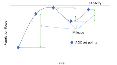
Figure 2: Illustration of the computation of capacity and mileage

[CP1]: Market clearance. All participating resources submit their capacity bids, capacity price bids, and mileage price bids to the RTO. Capacity bids are the maximum amount of regulation (up or down) that the resource can provide. Capacity price bids are the unit price of providing these regulations. Mileage is the sum of the absolute change in AGC set points, which corresponds to the summation of the vertical lines in Figure 2. The mileage price bid is the cost for unit change in regulation. Typically, expected mileages are calculated from historical data and resources do not submit mileage bids. The RTO clears the market with a capacity and mileage price that is uniform across the resources, and sends each resource its capacity and mileage allocation. This off-line process happens only once per regulation event.

[CP2]: Allocation of regulation signal to each resource. The RTO sends the regulation set points to each of the procured energy resources every 2-4 seconds for the entire regulation period, which is usually 10-15 minutes. The regulation set points are computed from the AGC signal in real time in proportion to the procured mileage of each resource. In case the assigned capacity of a resource is violated, the overshoot power is redistributed to the other resources in proportion to their assigned mileages.

[CP3]: Real-time tracking of regulation signal. Once the regulation set points have been assigned, the resources need to track them in real time.

Payment to the resources comprises of two components, capacity payment and mileage payment. The capacity payment is done based on the assigned capacity in [CP1] while the mileage payment is done based on the actual mileage provided which reflects the performance of the resources while tracking the assigned signal in [CP3].

III-A1 Limitations of Current Practice

The centralized way of assigning the set points to the resources in [CP2] relies on the fixed number of resources with fixed generation capacities procured in [CP1], which are available for the entire regulation period. This is problematic in the context of aggregators, as they are subject to variabilities and uncertainties associated with the DERs inside them. Even if the DERs inside the microgrid participating stay during the regulation period, the users inside the microgrid can change their power consumption, which in turn leads to changes in the effective regulation capacity. Furthermore, in current practice, there is no direct consideration of the operational costs of the resources, which may result in suboptimal power allocation. Instead, we argue that the assignment of the regulation signal should be done, at each time step, in a way that optimizes the aggregate cost functions of the resources and takes into account their (possibly dynamic) operational limits. We refer to this approach as the RTO-DERP coordination problem. This idea has also been pointed out in the past by CAISO for traditional energy resources, cf. [26]. The lack of robustness and the information sharing requirements of centralized schemes motivate the investigation of distributed schemes to solve the RTO-DERP coordination problem.

III-A2 Challenges for Frequency Regulation from Microgrids

Here we describe the challenges specific to microgrid participation in frequency regulation markets. First, note that solving the RTO-DERP coordination problem with microgrids requires the identification, or rather the abstraction, of aggregate cost functions and regulation capacity bounds based on the cost functions and flexibilities of their DERs. Second, the determination of capacity bids requires taking into account the uncertainties associated with the microgrids. There is a need to calculate bids for each regulation interval, as they might need to considerably change from one interval to the next. Even within a regulation interval itself, the power level of the uncontrollable nodes might vary significantly. Third, the determination of mileage bids has to take into account the dependency of ramp rates on the composition and participation of the individual DERs. The current method of calculating expected mileages in [CP1] makes sense for conventional resources as their ramp rates are fixed and historical data provides reliable accuracy. In the case of microgrids, individual resources may be changing over time and ramp rates might not remain constant as a result. Also, the performance of participating resources for one regulation period to another might be substantially different.

III-B Problem Statement

Consider $N$ microgrids, each controlled by an aggregator. To enable microgrid participation in the frequency regulation market, we focus on [CP1] and [CP2]. Based on the discussion in Section III-A, we formalize the following problems.

[P1]: Meaningful abstractions for the microgrid. To enable the submission of bids in [CP1], each aggregator needs to quantify the maximum up/down regulation capacity that the microgrid can provide, the unit cost of providing such regulation, and the ramp rate at which the microgrid can change its power level. Our first goal is therefore to provide meaningful abstractions for these objects, and cost functions and ramp rate functions of the microgrids for [P2] below, a problem we tackle in Section IV.

[P2]: RTO-DERP distributed coordination. The RTO-DERP coordination problem for computing the set points for each resource advocated for [CP2] consists of an economic dispatch problem with ramp rate constraints at every instant of the regulation interval. Formally, for $x_{r}$ regulation at a given time instant, we have

$${\min_{x}} f(x)=\sum\limits_{\operatorname{\operatorname{i}}=1}^{N}f_{\operatorname{\operatorname{i}}}(x_{\operatorname{\operatorname{i}}})$$ (2)

s.t. $$\sum_{\operatorname{\operatorname{i}}=1}^{N}x_{\operatorname{\operatorname{i}}}=x_{r}$$

$$\underline{x_{\operatorname{\operatorname{i}}}}\leq x_{\operatorname{\operatorname{i}}}\leq\overline{x_{\operatorname{\operatorname{i}}}}\quad\forall\operatorname{\operatorname{i}}$$

$$|x_{\operatorname{\operatorname{i}}}-x_{\operatorname{\operatorname{i}}}^{-}|\leq R_{\operatorname{\operatorname{i}}}(x_{\operatorname{\operatorname{i}}}^{-})\quad\forall\operatorname{\operatorname{i}},$$

where $x\in\mathbb{R}^{N}$ is the vector of regulation power from the microgrids, $f_{\operatorname{\operatorname{i}}}(x_{\operatorname{\operatorname{i}}})$ is the cost of $x_{\operatorname{\operatorname{i}}}$ regulation for microgrid $\operatorname{\operatorname{i}}$, $\underline{x_{\operatorname{\operatorname{i}}}}$ and $\overline{x_{\operatorname{\operatorname{i}}}}$ are the lower and upper bounds of regulation for microgrid ${\operatorname{\operatorname{i}}}$ which are bounded by the solutions of [P1] and determined by [CP1] for a specific regulation period, $x_{\operatorname{\operatorname{i}}}^{-}$ is the regulation that the microgrid $\operatorname{\operatorname{i}}$ was providing at the previous instant, and $R_{\operatorname{\operatorname{i}}}(x_{\operatorname{\operatorname{i}}})$ is the ramp rate of the microgrid when it is providing regulation $x_{\operatorname{\operatorname{i}}}$. Because of the ramp constraints present in (2), this problem might not be always feasible (since mileage requirements set by the RTO while clearing the market in [CP1] capture the average mileage required, and not the extreme cases). In such cases, we want to minimize the error between the procured regulation and the required one. We tackle these in Section V.

IV Microgrid Abstractions

Consider a microgrid with $n\in\mathbb{Z}_{>1}$ buses, described by $\operatorname{\mathcal{G}}_{m}=(\operatorname{\mathcal{V}},\operatorname{\mathcal{E}},\operatorname{\mathsf{A}})$. Without loss of generality, we assume that the first bus is connected to the bulk grid through a tie line. We partition the remaining set of buses as $\operatorname{\mathcal{V}}_{g}\cup\operatorname{\mathcal{V}}_{l}$, where $\operatorname{\mathcal{V}}_{g}$ is the set of controllable nodes and $\operatorname{\mathcal{V}}_{l}$ is the set of uncontrollable nodes (or loads). Let $n=|\operatorname{\mathcal{V}}|$, $n_{g}=|\operatorname{\mathcal{V}}_{g}|$, $n_{l}=|\operatorname{\mathcal{V}}_{l}|$ and $m=|\operatorname{\mathcal{E}}|$. Following [27], we assume that the lines connecting various buses inside the microgrid are lossless and inductive. In case the electrical lines inside the microgrid are lossy with sufficiently uniform resistance to reactance ratios, they could still be represented via a lossless model obtainable through a linear transformation [28]. Since the voltage dynamics governed by the voltage droop controllers operate at much faster scale than the secondary frequency regulation [29], we assume the voltage magnitude of every bus to be approximately 1 p.u. Further, we assume that the network and inverter filter dynamics are fast enough so that we can model them as power injections with no dynamics [30, 31]. We adopt the convention that the value of the power injection is negative if the device consumes power and vice versa. The power level of each controllable node $p\in\operatorname{\mathcal{V}}_{g}$ is denoted by $g_{p}$, with $g_{p}^{0}$ denoting the baseline generation/consumption. The power level of each uncontrollable node $q\in\operatorname{\mathcal{V}}_{l}$ is denoted by $l_{q}$. We denote the incoming power through the tie line by $P$ and its baseline value by $P^{0}$. When the microgrid provides frequency regulation, the value of the tie line power $P$ is

$$P=P^{0}+x,$$

where $x$ is the allocated AGC signal. Note that since we model $P$ as the incoming power from bulk grid, $x$ would be negative when the microgrid is providing up regulation. Following [32], the power injections for the microgrid are given by

$$\begin{bmatrix}P&g^{\top}&-l^{\top}\end{bmatrix}^{\top}=\operatorname{\mathsf{M}}B\text{sin}(\operatorname{\mathsf{M}}^{\top}\theta),$$ (3)

where $g\in\mathbb{R}^{n_{g}}$ and $l\in\mathbb{R}^{n_{l}}$ are the vectors of controllable and uncontrollable nodes, resp., $\operatorname{\mathsf{M}}\in\mathbb{R}^{n\times m}$ is the incidence matrix of the graph, $B\in\mathbb{R}^{m\times m}$ is the diagonal matrix of absolute line susceptances and $\theta\in\mathbb{R}^{n}$ is the vector of phase angles. Additionally, there is a constraint that the maximum phase angle difference between any two interconnected buses should be bounded by $\Theta\in_{\geq 0}$, i.e.,

$$|\theta_{i}-\theta_{k}|\leq\Theta.$$ (4)

To avoid dealing with the nonlinearity in (3), we assume $\operatorname{\mathcal{G}}_{m}$ is a graph with non-overlapping loops and rewrite the power flow equations as

$$\begin{bmatrix}P&g^{\top}&-l^{\top}\end{bmatrix}^{\top}=\operatorname{\mathsf{M}}\omega,$$ (5a)

$$\>|\omega|\leq\overline{\omega}.$$ (5b)

Here $\omega\in\mathbb{R}^{m}$ is the vector of line flows and $\overline{\omega}\in\mathbb{R}^{m}$ is the vector of maximum permissible flows. Since the columns of the fundamental loop matrix form a basis for the null space of the incidence matrix, cf. [33, Theorem 4-6], we write (5) as

$$\big{|}\operatorname{\mathsf{M}}^{+}\begin{bmatrix}\mathbf{1}^{\top}l-\mathbf{1}^{\top}g\\ g\\ -l\end{bmatrix}+\operatorname{\mathsf{N}}\gamma\big{|}\leq\overline{\omega},$$ (6)

where $\operatorname{\mathsf{M}}^{+}$ denotes the Moore-Penrose pseudoinverse of $\operatorname{\mathsf{M}}$, $\operatorname{\mathsf{N}}\in^{m\times(m-n+1)}$ is the fundamental loop matrix of $\operatorname{\mathcal{G}}_{m}$, and $\gamma\in^{m-n+1}$.

IV-A Capacity Bounds

The microgrid needs to solve an optimization problem to find the maximum up (or down) regulation that it can provide. For up regulation, the power consumption of the microgrid is less than the baseline power. Since the latter is constant for the regulation period, computing the capacity is equivalent to minimizing $P$ while satisfying the power flow constraints. If the power level of uncontrollable nodes is constant for the entire regulation period, then the problem reads as

$$\min_{g,\omega} P$$ (7)

s.t. $$\begin{bmatrix}P&g^{\top}&-l^{\top}\end{bmatrix}^{\top}=\operatorname{\mathsf{M}}\omega$$

$$\;\underline{g}\leq g\leq\overline{g},\quad|\omega|\leq\overline{\omega},$$

where $\underline{g}$ and $\overline{g}$ are the vectors of minimum and maximum possible power levels of controllable nodes, respectively. If $\underline{P}$ denotes the solution of (7), then the maximum up regulation is $\overline{x}=\underline{P}-P^{0}$. The maximum down regulation $\underline{x}$ can be obtained solving a similar maximization problem.

The formulation (7) assumes the power level of the uncontrollable nodes remains constant, and therefore does not take into account the varying nature of the loads. In practice, this makes sense for a specific regulation instant, and would rarely be the case for the whole regulation period. Instead, a more robust way of calculating the capacity bounds that the aggregator can use in bidding for the whole regulation period is to account for worst-case scenarios, i.e., taking the expected maximum value for the uncontrollable nodes while computing the maximum up regulation. Although robust to variations in the uncontrollable nodes’ powers, this way of computing capacity bounds might be too conservative and, in fact, might prohibit the microgrid from participating in the regulation market at all. As an alternative, we propose a reformulation of problem (7) based on chance constraints. Using (6), we rewrite the optimization problem (7) as

$$\min_{g,\gamma,t} t$$ (8)

s.t. $$t\geq\mathbf{1}^{\top}l-\mathbf{1}^{\top}g$$

$$\big{|}\operatorname{\mathsf{M}}^{+}\begin{bmatrix}\mathbf{1}^{\top}l-\mathbf{1}^{\top}g\\ g\\ -l\end{bmatrix}+\operatorname{\mathsf{N}}\gamma\big{|}\leq\overline{\omega}$$

$$\underline{g}\leq g\leq\overline{g}.$$

Assume that a probability distribution describing the power levels of uncontrollable nodes at any instant of the regulation period is available. To account for load variability, we instead consider the following chance-constrained optimization

$$\min_{g,\gamma,t} t$$

s.t. $$\Pr(t\geq\mathbf{1}^{\top}l-\mathbf{1}^{\top}g)\geq 1-\epsilon^{\prime}$$ (9)

$$\Pr\Big{(}\big{|}\operatorname{\mathsf{M}}^{+}\begin{bmatrix}\mathbf{1}^{\top}l-\mathbf{1}^{\top}g\\ g\\ -l\end{bmatrix}+\operatorname{\mathsf{N}}\gamma\big{|}_{j}\leq\overline{\omega}_{j}\Big{)}\geq 1-\epsilon\quad\forall j$$

$$\underline{g}\leq g\leq\overline{g}.$$

where $\epsilon^{\prime},\epsilon\in[0,1]$. In this formulation, each flow constraint can be violated, with a probability no more than $\epsilon$.

Since the regulation period lasts for only a short period of time (10-15 minutes), the variation in the loads would not be significant and it is reasonable to assume it could be approximately characterized by a normal distribution. The next result, whose proof is in the Appendix, shows that the chance-constrained optimization (IV-A) can be solved via a deterministic linear program if the loads are normally distributed.

Lemma IV.1.

(Capacity bounds for variable loads via deterministic optimization): Assume the loads are distributed normally with mean $\hat{l}$ and variance $V_{l}$. Then, the solution of the deterministic linear program

$$\min_{g,\gamma,t} t$$ (10)

s.t. $$\mathbf{1}^{\top}\hat{l}-\mathbf{1}^{\top}g-t\leq\sqrt{2}\operatorname{\operatorname{erf}}^{-1}(2\epsilon^{\prime}-1)(\mathbf{1}^{\top}V_{l}\mathbf{1})^{1/2}$$

$$|(\operatorname{\mathsf{M}}_{1}\mathbf{1}^{\top}-\operatorname{\mathsf{M}}_{3})\hat{l}+(\operatorname{\mathsf{M}}_{2}-\operatorname{\mathsf{M}}_{1}\mathbf{1}^{\top})g+\operatorname{\mathsf{N}}\gamma|\leq\overline{\omega}^{l}$$

$$\underline{g}\leq g\leq\overline{g},$$

where $\operatorname{\mathsf{M}}^{+}=[\operatorname{\mathsf{M}}_{1}\quad\operatorname{\mathsf{M}}_{2}\quad\operatorname{\mathsf{M}}_{3}]$ with $\operatorname{\mathsf{M}}_{1}\in^{m}$, $\operatorname{\mathsf{M}}_{2}\in^{m\times n_{g}}$ and $\operatorname{\mathsf{M}}_{3}\in^{m\times n_{l}}$, $\overline{\omega}^{l}=\overline{\omega}+K$ and

$$K_{j}=\sqrt{2}\operatorname{\operatorname{erf}}^{-1}(\epsilon-1)\cdot\\ \cdot\big{(}(\operatorname{\mathsf{M}}_{1j}\mathbf{1}^{\top}-\operatorname{\mathsf{M}}_{3j})V_{l}(\operatorname{\mathsf{M}}_{1j}\mathbf{1}^{\top}-\operatorname{\mathsf{M}}_{3j})^{\top}\big{)}^{1/2},$$

is a solution of problem (IV-A).

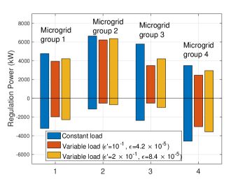
Figure 3: Regulation capacities for different instantiations of the reduced-order UCSD microgrid. The 12 microgrids are divided into 4 groups, with constant mean value of loads and baseline generation across each group. Within each group, for the first scenario, the variance is 0 and for the remaining two scenarios, it is given by the diagonal matrix which is 0.25 times the squared value of mean loads. Values of $\epsilon^{\prime},\epsilon$ for the second and third scenarios are $10^{-1},4.2\times 10^{-5}$ and $2\times 10^{-1},8.4\times 10^{-5}$, respectively.

We use Lemma IV.1 to compute in Figure 3 the maximum up and down regulation for several microgrids modeled after the reduced-order UCSD microgrid described later in Section VI. The microgrids are divided into 4 groups, each with a different value of baseline generation and mean load for the UCSD model. Within each group, we consider 3 different scenarios, one with constant load and the other two with varying loads (generated using the same normal distribution with variance equal to a diagonal matrix given by 0.25 times the squared value of mean loads) and different confident values ($\epsilon^{\prime},\epsilon=10^{-1},4.2\times 10^{-5}$ and $2\times 10^{-1},8.4\times 10^{-5}$, respectively). One can see in Figure 3 that the capacity bounds increase with $\epsilon^{\prime},\epsilon$, which is in agreement with the fact that larger values of these correspond to lower probability of satisfying the constraints.

Note that the probabilistic capacity bounds identified above and obtained after solving (10) are good only for the bidding in [CP1]. The actual regulation bounds at a given regulation instant still depend on the load at that instant.

IV-B Ramp Rate Function

In the following we discuss how to compute the ramp up rate for the microgrid (the discussion for ramp down rate is analogous). If there were no constraints on the power flows, then the ramp rate of the microgrid would be the summation of ramp rates of all the controllable nodes. However, the presence of flow constraints may prevent every controllable node from ramping at its full capacity and as such, the ramp rate is a function that depends on the operating point of the controllable nodes. Let $\operatorname{\mathcal{F}}_{g}=\{g\in^{n_{g}}\;|\;\exists\;\omega\in^{m}\text{ satisfying~{}\eqref{eq:pff}}\}$ denote the set of feasible operating points for controllable nodes. If the power levels of the uncontrollable nodes are constant, then the ramp up rate, $\operatorname{\mathcal{R}}:\operatorname{\mathcal{F}}_{g}\to_{\geq 0}$, is formally given by

$$\max_{\Delta g,\Delta\omega} \mathbf{1}^{\top}\Delta g$$ (11)

s.t. $$\begin{bmatrix}(P-\mathbf{1}^{\top}\Delta g)&(g+\Delta g)^{\top}&-l^{\top}\end{bmatrix}^{\top}=\operatorname{\mathsf{M}}(\omega+\Delta\omega)$$

$$\Delta g\leq r,\quad|\omega+\Delta\omega|\leq\overline{\omega},$$

where $r\in^{n_{g}}$ is the vector whose component $r_{p}$ is the nominal ramping capacity of the controllable node $p$, and $\omega+\Delta\omega$ is the vector of line flows corresponding to the operating point $g+\Delta g$.

If the power levels of the uncontrollable nodes are variable, we use chance-constraints as in the case of capacity bounds and the ramp up rate $\operatorname{\mathcal{R}}$ is given by

$$\max_{\Delta g,\gamma} \mathbf{1}^{\top}\Delta g$$ (12)

s.t. $$\Pr\Big{(}\big{|}\operatorname{\mathsf{M}}^{+}\!\!\begin{bmatrix}\operatorname{\mathbf{1}}^{\top}l-\operatorname{\mathbf{1}}^{\top}(g+\Delta g)\\ g+\Delta g\\ -l\end{bmatrix}\!\!+\operatorname{\mathsf{N}}\gamma\big{|}_{j}\leq\overline{\omega}_{j}\Big{)}\geq 1-\epsilon\;\forall j$$

$$\Delta g\leq r.$$

The following result, whose proof is similar to that of Lemma IV.1 and omitted to avoid repetition, converts the chance-constrained optimization (12) into a deterministic linear program if the loads are normally distributed.

Lemma IV.2.

(Ramp rate for variable loads via deterministic optimization): Assume the loads are distributed normally with mean $\hat{l}$ and variance $V_{l}$. Then, the solution of the deterministic linear program

$$\max_{\Delta g,\gamma} \operatorname{\mathbf{1}}^{\top}\Delta g$$ (13)

s.t. $$|(\operatorname{\mathsf{M}}_{1}\operatorname{\mathbf{1}}^{\top}-\operatorname{\mathsf{M}}_{3})\hat{l}+(\operatorname{\mathsf{M}}_{2}-\operatorname{\mathsf{M}}_{1}\operatorname{\mathbf{1}}^{\top})(g+\Delta g)+\operatorname{\mathsf{N}}\gamma|\leq\overline{\omega}^{l}$$

$$\Delta g\leq r,$$

where $\operatorname{\mathsf{M}}_{1}$, $\operatorname{\mathsf{M}}_{2}$, $\operatorname{\mathsf{M}}_{3}$ and $\overline{\omega}^{l}$ are as defined in Lemma IV.1, is a solution for problem (12).

The next result states the properties of the ramp rate function (11) for a tree network. The proof, given in the Appendix, is based on the description of the feasible region in terms of the power levels of the controllable nodes stated in Lemma .1. For the ramp rate function with normally distributed loads defined in (12), one can obtain a similar result following Lemma IV.2 (with $\overline{\omega}$ replaced by $\overline{\omega}^{l}$).

Proposition IV.3.

(Ramp rate of tree network): Let $\operatorname{\mathcal{G}}_{m}$ be a tree and $H$ denote the hyperrectangle describing the region of operation of the controllable nodes, where opposite faces correspond to the minimum and maximum possible power level of a controllable node. Then the ramp rate $\operatorname{\mathcal{R}}$ is piecewise affine on $H$, i.e., for some $s>0$, $H$ admits a decomposition

$$H=V_{1}\cup V_{2}\cup\ldots\cup V_{s},$$

where $\{V_{\alpha}\}_{\alpha=1}^{s}$ are polyhedra, and $\operatorname{\mathcal{R}}$ is affine on each $V_{\alpha}$.

Remark 1.

(Ramp rate for networks with non-overlapping loops): If the network is not a tree, then the flows corresponding to a power injection vector are not unique. Nevertheless, the ramp rate for networks with non-overlapping loops is a non-increasing function of $g$, as the feasible region of (11) can only shrink with increase in some component(s) of $g$. $\bullet$

Given a regulation power $x$, we note that there may be more than one feasible operating point for the microgrid that produces it. As a result, the ramp rate as a function of regulation power is not uniquely defined. We address this by defining $R:[\overline{x},\underline{x}]\to_{\geq 0}$, as

$$R(x)={\max\limits_{g^{*}}}\>\operatorname{\mathcal{R}}(g^{*}),$$

where $g^{*}$ denotes a minimizer of the cost of producing the regulation $x$ while respecting the power flow and capacity constraints. We take the maximum, since the optimizer $g^{*}$ might not be unique. If the cost functions for all the controllable nodes are convex, each $g^{*}$ is a decreasing function with respect to $x$, which means that at least one component of $g^{*}$ would decrease as $x$ increases (using the convention that up regulation is negative). Using this fact, we conclude that $R$ as a function of $x$ is non-decreasing, with maximum possible value as $\mathbf{1}^{\top}r$. Figure 4 provides the ramp rate functions of the four groups of microgrids displayed in Figure 3 in the constant load case.

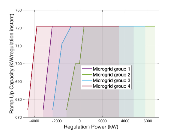
Figure 4: Ramp rate functions for different instantiations of the reduced-order UCSD microgrid with constant loads. The shaded regions represent the range of regulation power that the corresponding microgrid can provide.

In Remark 2, we discuss the conditions under which the minimum ramp rate of the microgrid is always non-zero.

Remark 2.

(Non-zero minimum ramp rate): It is natural to argue that the microgrid could have a zero minimum ramp rate. Here, we discuss conditions under which the minimum ramp rate of the microgrid is non-zero. Let $\operatorname{\mathcal{E}}^{\prime}=\{e_{j}\in\operatorname{\mathcal{E}}\;|\;\omega_{j}<\overline{\omega}_{j}\}$ be the set of all the lines which have not reached their flow limits when providing the maximum up regulation. Next, consider the graph $\operatorname{\mathcal{G}}_{m}^{\prime}=(\operatorname{\mathcal{V}},\operatorname{\mathcal{E}}^{\prime})$ and let $\operatorname{\mathcal{V}}^{\prime}_{g}=\{v_{i}\in\operatorname{\mathcal{V}}_{g}\;|\;\exists\text{ a path from }i\text{ to }1\text{ in }\operatorname{\mathcal{G}}_{m}\}$, i.e., the set of controllable nodes which are connected to the tie line. If $\operatorname{\mathcal{V}}^{\prime}_{g}\neq\phi$, then the minimum ramp rate is always non-zero. $\bullet$

IV-C Cost Function

Each aggregator needs to calculate the cost of providing a given amount of regulation by capturing the effect of operating the controllable nodes away from their baseline operating points. For an operating point $g$, the total cost for the aggregator is given by

$$h(g)=\sum_{p\in\operatorname{\mathcal{V}}_{g}}h_{p}(g_{p}),$$ (14)

where $h_{p}:\to_{\geq 0}$ is the cost of operating node $p$ away from its baseline level $g_{p}^{0}$. One representative example of such a function is $h_{p}(g_{p})=(g_{p}-g_{p}^{0})^{2}$. The total regulation that the aggregator provides is the combination of individual regulations of controllable nodes. Therefore, for a specified regulation level $x$, one would ideally choose the value of $g$ that minimizes the total cost given by (14) respecting the power flow constraints in (5) and the minimum and maximum capacity constraints on each controllable node. Formally, $f:[\overline{x},\underline{x}]:\to_{\geq 0}$, is given by

$$f(x)=\begin{cases}\begin{aligned} &{\min_{g,\omega}}&&h(g)\\ &\text{s.t.}&&\underline{g}\leq g\leq\overline{g}\\ &&&\begin{bmatrix}(P^{0}+x)&g^{\top}&-l^{\top}\end{bmatrix}^{\top}=\operatorname{\mathsf{M}}\omega\\ &&&|\omega|\leq\overline{\omega}.\end{aligned}\end{cases}$$ (15)

However, a cost function defined like this does not take into account the previous operating point of the microgrid and assumes that it can transition between the optimal points corresponding to different regulation powers arbitrarily fast. In practice, however, since the regulation set points change every 2-4 seconds, ramp rates might limit the change from optimal point at one time instant to the next. This suggests that the cost of providing certain amount of regulation at one instant also depends on the value of the regulation power at the previous instant. Hence, we define the cost $\mathbf{f}:[\overline{x},\underline{x}]\times[\overline{x},\underline{x}]\to_{\geq 0}$, of providing regulation power $x$, if providing regulation power $x^{-}$ at the previous instant, as

$$\min\limits_{g,\Delta g,\omega,\Delta\omega} h(g+\Delta g)$$

s.t. $$\underline{g}\leq g+\Delta g\leq\overline{g},\quad\Delta g\leq r$$ (16)

$$\begin{bmatrix}(P^{0}+x)&(g+\Delta g)^{\top}&-l^{\top}\end{bmatrix}^{\top}=\operatorname{\mathsf{M}}(\omega+\Delta\omega)$$

$$|\omega+\Delta\omega|\leq\overline{\omega}$$

$$\underline{g}\leq g\leq\overline{g}\quad|\omega|\leq\overline{\omega}$$

$$\begin{bmatrix}(P^{0}+x^{-})&g^{\top}&-l^{\top}\end{bmatrix}^{\top}=\operatorname{\mathsf{M}}\omega.$$

Here, $(g+\Delta g,\omega+\Delta\omega)$ and $(g,\omega)$ are the vectors of the power levels of controllable nodes and line flows when the microgrid provides regulation power $x$ and $x^{-}$, respectively. The constraints also enforce the capacity limits for the individual controllable nodes and the flow limit constraints for both values of regulation power, and the ramp constraints in transitioning from $x^{-}$ to $x$. The reason to include the power flow constraints at $x^{-}$ in (IV-C) is to enable the aggregator to pre-compute the cost function independently of the regulation power it might be asked to provide. Otherwise, if the cost is computed at every regulation instant, $g$ and $\omega$ providing $x^{-}$ would be known, and the optimization variables would only be $\Delta g$, and $\Delta\omega$. As such, $\mathbf{f}(x,x^{-})$ is a lower bound on the actual cost since $(g,\omega)$ are also decision variables and are selected optimally to move to the next operating point.

The following result, whose proof is given in the Appendix, identifies a condition that simplifies the computation of the cost function $\mathbf{f}(x,x^{-})$ defined in (IV-C).

Lemma IV.4.

(Simplified formulation and convexity of cost function): Given regulation powers $x^{-}$ and $x$, if $|x-x^{-}|\leq R(x^{-})$, then $\mathbf{f}(x,x^{-})=f(x)$. If $h$ is (strictly) convex, then $f$ is (strictly) convex.

Figure 5 provides the cost functions (15) of the four groups of microgrids displayed in Figure 3 in the constant load case.

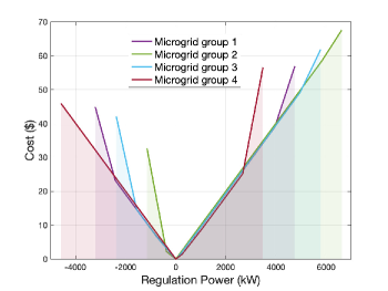
Figure 5: Abstracted cost functions for different instantiations of the reduced-order UCSD microgrid with constant loads. The shaded regions represent the range of regulation power that the corresponding microgrid can provide.

Note that the cost function (15) assumes the load to be constant, but since the aggregator is not required to submit its cost functions in [CP1], there is no need to pre-compute this using probabilistic techniques. Instead, the cost function at a given regulation instant could be computed online using the load at that instant. The time taken to compute the cost function at a given instant would depend upon the type of solver used, but is usually small (e.g., less than a second with built in MATLAB solver fmincon). In addition, since the regulation period lasts for 10-15 minutes, the variation in load would be limited, thereby requiring the recomputation of the cost function sparingly.

IV-D Bids for Participation in Market Clearance

Based on the abstractions in Sections IV-A-IV-C, here we specify the bid information used by each aggregator to participate in [CP1]. Without loss of generality, we specify the bid quantities for up regulation market. Let $g^{\text{up}}\in^{n_{g}}$ denote the component in $g$ of the solution of (7).

TABLE I: Bidding quantities for up regulation market

Bid Quantity	Value
Capacity	$|\overline{x}|$
Mileage	$k\operatorname{\mathcal{R}}(g^{\text{up}})$
Capacity price	$h(g^{\text{up}})/|\overline{x}|$

Table I specifies the proposed values for the bidding quantities. Here $k>0$ is a constant depending on the duration of the regulation period and update frequency of the AGC setpoints. The suggested bids are conservative, meaning that the aggregator would be able to provide whatever it promises, and there is no strategy to maximize profit. It might seem from Table I that there is no need to compute beforehand the whole ramp rate function $\operatorname{\mathcal{R}}$ in Section IV-B. However, a risk taking aggregator might use a higher value of mileage bid based on the shape of $\operatorname{\mathcal{R}}$. It is also interesting to note that, from the convexity of cost function in Lemma IV.4 and the capacity price bid in Table I, the aggregator would never be at loss regardless of the regulation power being provided.

V RTO-DERP Coordination Problem

Here we describe our algorithmic solution for the RTO-DERP coordination problem [P2] to disaggregate the regulation signal. Equipped with the microgrids’ capacities and cost and ramp rate functions identified in Section IV, the aggregators, communicating over a graph $\operatorname{\mathcal{G}}$, seek to solve, at each instant of the regulation period, the optimization problem (2). However, as we have noted before, this problem might not always be feasible due to the presence of ramp constraints. This means that in principle, at each regulation instant, one would need to solve (2) if it is feasible or minimize the difference between the required regulation and the procured regulation if it is infeasible. Such dichotomy also raises the issue of the necessary information available to the aggregators to determine which one of the two cases to address at each regulation instant.

Instead, we propose to reformulate the optimization problem in a way that lends itself to the identification of solutions that minimize the error between the procured regulation and the required regulation whenever (2) is not feasible. Without loss of generality, throughout this section we assume the required regulation power to be positive. We start by defining the problem

$${\min_{x}} f^{\mu}(x)=f(x)+\mu[\Delta x]^{+}$$ (17)

s.t. $$\underline{x_{\operatorname{\operatorname{i}}}}\leq x_{\operatorname{\operatorname{i}}}\leq\overline{x_{\operatorname{\operatorname{i}}}}\quad\forall\operatorname{\operatorname{i}}$$

$$|x_{\operatorname{\operatorname{i}}}-x_{\operatorname{\operatorname{i}}}^{-}|\leq R_{\operatorname{\operatorname{i}}}(x_{\operatorname{\operatorname{i}}}^{-})\quad\forall\operatorname{\operatorname{i}},$$

where $\mu>0$ is a penalty parameter and $\Delta x=x_{r}-\operatorname{\mathbf{1}}^{\top}x$. The following result, whose proof is given in the Appendix, characterizes the equivalence between problems (17) and (2).

Lemma V.1.

(Equivalence between (2) and (17)): Optimization (17) is always feasible and there exists $\hat{\mu}<\infty$ such that for all $\mu\in[\hat{\mu},\infty)$,  (2) and (17) have the same solution set if (2) is feasible.

Remark 3.

(Establishing the threshold value $\hat{\mu}$ without the knowledge of dual optimizers): The threshold value $\hat{\mu}$ in Lemma V.1 depends on the optimal values of the dual variables, which is not known beforehand. Interestingly, the explicit knowledge of the Lagrange multipliers to obtain a lower bound on the value of $\mu$ can be avoided. In fact, according to [34, Proposition 5.2], we have

$$\hat{\mu}\geq 2\max\limits_{x\in\mathcal{F}}\|\nabla f(x)\|_{\infty}. \bullet$$

Given Lemma V.1, we focus on solving problem (17) in a distributed way. To handle the local constraints, we again reformulate (17) using exact penalty function as

$$\min\limits_{x}\;f^{p}(x)= \underbrace{f(x)+\mu_{2}\sum\limits_{\operatorname{\operatorname{i}}=1}^{N}\big{(}[\overline{b_{\operatorname{\operatorname{i}}}}]^{+}+[\underline{b_{\operatorname{\operatorname{i}}}}]^{+}\big{)}}_{f^{\mu_{2}}(x)}+\mu[\Delta x]^{+},$$ (18)

$$\text{where }\overline{b_{\operatorname{\operatorname{i}}}}= x_{\operatorname{\operatorname{i}}}-\min\{\overline{x_{\operatorname{\operatorname{i}}}},x_{\operatorname{\operatorname{i}}}^{-}+R_{\operatorname{\operatorname{i}}}(x_{\operatorname{\operatorname{i}}}^{-})\},$$

$$\text{and }\underline{b_{\operatorname{\operatorname{i}}}}= \max\{\underline{x_{\operatorname{\operatorname{i}}}},x_{\operatorname{\operatorname{i}}}^{-}-R_{\operatorname{\operatorname{i}}}(x_{\operatorname{\operatorname{i}}}^{-})\}-x_{\operatorname{\operatorname{i}}},$$

are the box constraints taking care of the capacity and ramp rate for aggregator $\operatorname{\operatorname{i}}\in\{1,\ldots,N\}$ and $\mu_{2}>0$ is again a penalty parameter. Once again, similar to Lemma V.1, there exist finite values of $\mu_{2}$ for which the reformulation (18) is exact.

Since problem (18) is unconstrained, consider the dynamics

$$\dot{x}\in-\partial f^{p}(x),$$ (19)

where $\partial f^{p}:^{N}\rightrightarrows^{N}$ denotes the generalized gradient of $f^{p}$. For each agent $\operatorname{\operatorname{i}}\in\{1,\ldots,N\}$, $[\partial f^{p}(x)]_{\operatorname{\operatorname{i}}}$ is given by

$$\begin{cases}\nabla f_{\operatorname{\operatorname{i}}}(x_{\operatorname{\operatorname{i}}})-[\mu]^{+}_{\Delta x}-[\mu_{2}]^{+}_{\overline{b_{i}}}+[\mu_{2}]^{+}_{\underline{b_{i}}},&\Delta x,\overline{b_{\operatorname{\operatorname{i}}}},\underline{b_{\operatorname{\operatorname{i}}}}\neq 0,\\ \nabla f_{\operatorname{\operatorname{i}}}(x_{\operatorname{\operatorname{i}}})-[0,\mu]-[\mu_{2}]^{+}_{\overline{b_{i}}}+[\mu_{2}]^{+}_{\underline{b_{i}}},&\Delta x=0,\overline{b_{\operatorname{\operatorname{i}}}},\underline{b_{\operatorname{\operatorname{i}}}}\neq 0,\\ \nabla f_{\operatorname{\operatorname{i}}}(x_{\operatorname{\operatorname{i}}})-[\mu]^{+}_{\Delta x}-[0,\mu_{2}]+[\mu_{2}]^{+}_{\underline{b_{i}}},&\Delta x,\underline{b_{\operatorname{\operatorname{i}}}}\neq 0,\overline{b_{\operatorname{\operatorname{i}}}}=0,\\ \nabla f_{\operatorname{\operatorname{i}}}(x_{\operatorname{\operatorname{i}}})-[\mu]^{+}_{\Delta x}-[\mu_{2}]^{+}_{\overline{b_{\operatorname{\operatorname{i}}}}}+[0,\mu_{2}],&\Delta x,\overline{b_{\operatorname{\operatorname{i}}}}\neq 0,\underline{b_{\operatorname{\operatorname{i}}}}=0,\\ \nabla f_{\operatorname{\operatorname{i}}}(x_{\operatorname{\operatorname{i}}})-[0,\mu]-[0,\mu_{2}]+[\mu_{2}]^{+}_{\underline{b_{i}}},&\Delta x,\overline{b_{\operatorname{\operatorname{i}}}}=0,\underline{b_{\operatorname{\operatorname{i}}}}\neq 0,\\ \nabla f_{\operatorname{\operatorname{i}}}(x_{\operatorname{\operatorname{i}}})-[0,\mu]-[\mu_{2}]^{+}_{\overline{b_{i}}}+[0,\mu_{2}],&\Delta x,\underline{b_{\operatorname{\operatorname{i}}}}=0,\overline{b_{\operatorname{\operatorname{i}}}}\neq 0.\end{cases}$$

The equilibria of the dynamics (19) satisfy $\operatorname{\mathbf{0}}\in\partial f^{p}(x)$. Asymptotic convergence of (19) to the optimizers of (18) could be easily established using tools from non-smooth analysis, cf. [35, Proposition 14]. However, the implementation of (19) requires every aggregator to have the knowledge of the total regulation at all times. To handle this, we use dynamic average consensus, cf. Section II, to estimate the average of the difference between the required regulation and procured regulation from all the microgrids. Since $\frac{1}{N}\Delta x$ and $\Delta x$ have the same signs, we modify algorithm (19) using dynamic average consensus as follows

$$\!\!\dot{x} \in-\partial f^{\mu_{2}}(x)+[\mu]_{z}^{+},$$ (20a)

$$\!\!\dot{z} \in-\nu z-\beta\operatorname{\mathsf{L}}z-v+\nu(x_{r}e-x)+\partial f^{\mu_{2}}(x)-[\mu]^{+}_{z},$$ (20b)

$$\!\!\dot{v} =\nu\beta\operatorname{\mathsf{L}}z,$$ (20c)

where $\operatorname{\mathsf{L}}\in^{N\times N}$ is the Laplacian matrix of $\operatorname{\mathcal{G}}$, $z,v\in^{N}$, $z_{\operatorname{\operatorname{i}}}$ is the $\operatorname{\operatorname{i}}$th aggregator’s estimate of $\frac{1}{N}\Delta x$, $[\mu]^{+}_{z}\in^{N}$ with its $\operatorname{\operatorname{i}}$th element as $[\mu]^{+}_{z_{\operatorname{\operatorname{i}}}}$ and $e$ is the unit vector with only one entry as one and all others as zero. Note immediately that the algorithm (20) is distributed over the communication graph and only one aggregator needs to know the required regulation. We refer to (20) as “gradient descent + dynamic average consensus” algorithm, abbreviated as $\psi_{\text{gdac}}$. The equilibria for $x$ are the points satisfying $\operatorname{\mathbf{0}}\in-\partial f^{\mu_{2}}(x)+[\operatorname{\mathbf{0}},\mu\operatorname{\mathbf{1}}]$. The next result, whose proof is given in the Appendix, characterizes the convergence properties of the $\psi_{\text{gdac}}$ algorithm.

Theorem V.2.

(Asymptotic convergence of the distributed dynamics to the optimizers): Let $\operatorname{\mathcal{G}}$ be strongly connected and weight-balanced, and the initial conditions satisfy $\operatorname{\mathbf{1}}^{\top}v(0)=0$ and $\operatorname{\mathbf{1}}^{\top}z(0)-\Delta x(0)=0$, then there exists $\bar{\mu}<\infty$ such that the dynamics $\psi_{\text{gdac}}$ find the optimizers of (18) for all $\mu\in[\bar{\mu},\infty)$.

Remark 4.

(Initialization of the distributed algorithm): For the dynamics $\psi_{\text{gdac}}$ to converge to the optimizers, Theorem V.2 specifies requirements on the initial conditions. The requirement $\operatorname{\mathbf{1}}^{\top}v(0)=0$ could be implemented trivially by selecting $v(0)=\mathbf{0}$. For the implementation of $\operatorname{\mathbf{1}}^{\top}z(0)-\Delta x(0)=0$, the aggregators can simply choose $z(0)=\operatorname{\mathbf{0}}$ and $x_{\operatorname{\operatorname{i}}}(0)=0$ for all $\operatorname{\operatorname{i}}$, except for the aggregator who knows the required regulation for which $x_{\operatorname{\operatorname{i}}}(0)=x_{r}$. $\bullet$

VI Simulations

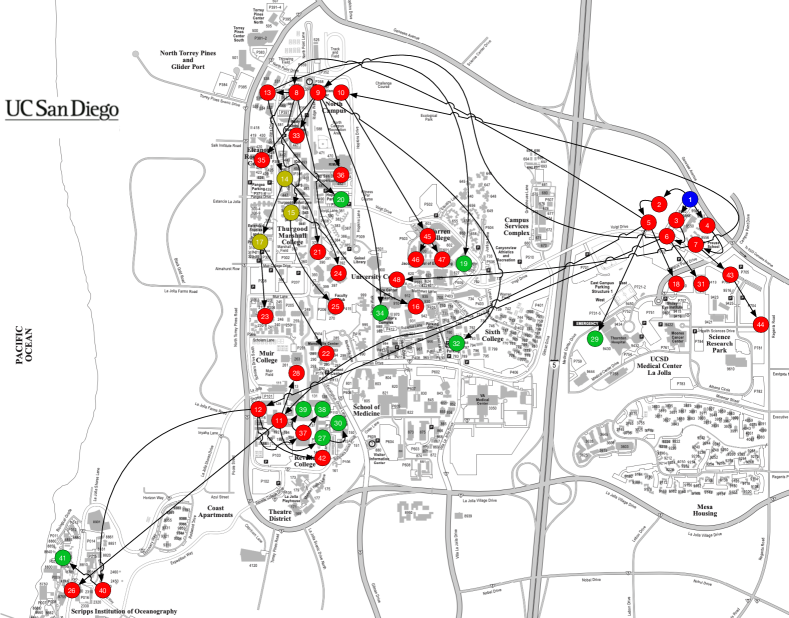
Figure 6: Reduced-order model of the UCSD microgrid. Arrowheads represent the direction of positive flows. Blue node (1) is connected to the tie line. Green nodes (19, 20, 27, 29, 30, 32, 34 38, 39 and 41) represent the generators, dark yellow (14, 15 and 17) the electric vehicle stations and red (remaining) the building loads.

We provide here our simulation results based on the abstractions of capacities, cost, and ramp rate developed in Section IV and the RTO-DERP coordination algorithm (20) in Section V. For the purpose of simulations, we consider a reduced-order model of the University of California, San Diego (UCSD) microgrid developed using the distributor feeder reduction algorithm in [36] and provided by the research group of Prof. Jan Kleissel. Compared to the full-order model of the UCSD microgrid [37] which is a radial, balanced network with 1289 buses (3869 nodes), the reduced-order model is a balanced tree network with 48 buses. The buses in the reduced-order model are obtained by retaining the key buses in the full order model which are the buses where the building loads aggregate or which have generators. Since the UCSD reduced-order model is balanced, we consider only one phase in our simulations. The model consists of 10 generators (2 gas turbines, 1 steam turbine, and 7 solar PV systems) and 37 loads (34 building loads and 3 electric vehicle stations). We show the location of the buses on the geographical map of the campus in Figure 6. For our simulation, we take the UCSD microgrid as a template, and we instantiate it using different baseline scenarios to construct 12 different microgrids, divided into 4 groups. The baseline values of generation and mean load is constant within a group. The 3 different scenarios within a group consist of (a) constant load, (b) variable load with failure probabilities $\epsilon^{\prime}=10^{-1}$, $\epsilon=4.2\times 10^{-5}$ and (c) variable load with failure probabilities $\epsilon^{\prime}=2\times 10^{-1}$, $\epsilon=8.4\times 10^{-5}$. The abstracted regulation capacities and ramp rate functions of different microgrid groups are shown in Figures 3 and 4, resp. For cost functions, we consider quadratics for all the resources. The abstracted cost functions for different groups are shown in Figure 5.

We demonstrate the performance of the distributed algorithm (20) in two sets of simulations. To implement the continuous-time algorithm, we use a first-order Euler discretization with step size of 0.001 to show its practical feasibility. The values of $\mu$, $\mu_{2}$, $\beta$ and $\nu$ are taken to be 1000, 1100, 400 and 400, respectively. In the first simulation, cf. Figure 7, we consider one regulation instant and first show the evolution of the proposed algorithm for required down regulation of 50000 kW, and compare it, for the same communication topology (undirected ring with few additional edges), against the (2-hop distributed) saddle-point dynamics [38] of the augmented Lagrangian for the equivalent reformulated problem as per [39]. As can be seen from the plots, the algorithm time required by the proposed algorithm to reach 1% band of the required regulation power in much less compared to the saddle-point dynamics. The time required does increase when the communication topology is changed to a directed ring - which is the worst possible topology for strongly connected graphs, but still remains less than a second, implying that the number of iterations is less than 1000.

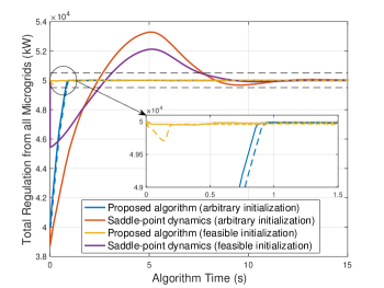
Figure 7: Performance of the proposed distributed algorithm compared against the saddle-point dynamics for 50000 kW down regulation from 12 aggregators. The dashed lines for the proposed algorithm represent the algorithm evolution over a directed ring, and the black dashed lines represent 1% band of the required regulation power. Dynamics were implemented in discrete time with a step size of 0.001 and the values of $\mu$, $\mu_{2}$, $\beta$ and $\nu$ as 1000, 1100, 400 and 400, respectively.

For the second simulation, we consider the dynamic regulation test signal (RegD), available on the Pennsylvania-New Jersey-Maryland Interconnection (PJM) website [40]. Since the RegD signal on the PJM website is normalized and could be scaled as long as the problem remains feasible, we scale it by a factor of 50000 and then use our abstractions and clear the market according to [CP1]. Once the market is cleared, we use our algorithm to track the scaled RegD signal and compare it using the current algorithm of disaggregating the regulation signal described in [CP2]. For the sake of clarity, we show only the first 100 instants of the regulation period, and instead of contributions from each of the 12 microgrids, show the total contributions from the 4 groups. As we can see from Figure 8, when it is not possible to provide the required amount due to limits on ramp rates, both the proposed algorithm and the current algorithm try to provide as much regulation power as possible, and the tracking performance for both the algorithms is similar. But, if we compare the cost, the proposed algorithm with a cost of $9104 outperforms the current algorithm with a cost of $9638. This difference in cost comes from very different power contributions from the microgrids for the two algorithms. The proposed algorithm allocates the regulation signal to the microgrids based on their abstracted cost functions (cf. Figure 5), whereas current practice does not take them into account. It can be noticed in Figure 8 that, under current practice, if not capped by the cleared capacities, the power allocations for different microgrid groups have the same ratios for every regulation instant. For example, the shape of the regulation power curves for microgrid groups 1, 3 and 4 are similar and only differ in terms of scaling (by factors depending on the ratio of their procured mileages).

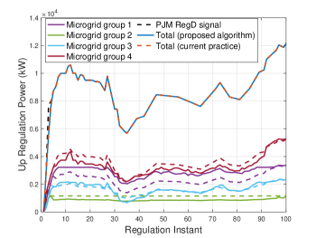
Figure 8: Performance of the proposed RTO-DERP coordination algorithm and the algorithm followed currently tested against first 100 updates of the PJM RegD signal. For microgrid groups, the solid lines represent the regulation power using the proposed algorithm and the dashed lines represent the regulation power using current practice. Although the tracking performance for both the algorithms is similar, contributions from individual microgrids differ substantially resulting into different costs.

VII Conclusions

We have considered the problem of providing frequency regulation services by aggregations of DERs. We have described the limitations of current practice and identified the challenges to overcome them with DER aggregators modeled as microgrids. We have developed meaningful abstractions for the capacity, cost of generation, and ramp rates by taking into account the power flow equations inside the microgrid. This provides enough information for the microgrids to participate in the market clearance stage. We have employed these abstractions to design a provably correct distributed algorithm that solves the RTO-DERP coordination problem to optimally disaggregate the regulation signal when the problem is feasible and minimize the difference between the required regulation and procured regulation when it is infeasible. Future work will extend our work to microgrids with more general topologies, incorporate AC power flow equations, and investigate smooth distributed algorithms to remove any chattering due to non-smooth dynamics.

Here we provide proofs of all the results stated in the paper.

Proof of Lemma IV.1

With the notation of the statement, (6) can be written as

$$\begin{vmatrix}\operatorname{\mathsf{M}}_{1}(\mathbf{1}^{\top}l-\mathbf{1}^{\top}g)+\operatorname{\mathsf{M}}_{2}g-\operatorname{\mathsf{M}}_{3}l+\operatorname{\mathsf{N}}\gamma\end{vmatrix}\leq\overline{\omega}.$$

Without loss of generality, let us for now consider only the following constraint in (IV-A)

$$\Pr(|\zeta_{j}|-\overline{\omega}_{j}\leq 0)\geq 1-\epsilon.$$ (21)

where $\zeta_{j}=(\operatorname{\mathsf{M}}_{1j}\mathbf{1}^{\top}-\operatorname{\mathsf{M}}_{3j})l+(\operatorname{\mathsf{M}}_{2j}-\operatorname{\mathsf{M}}_{1j}\mathbf{1}^{\top})g+\operatorname{\mathsf{N}}_{j}\gamma$. Let $\xi_{j}^{+}=\{\zeta_{j}\in\;|\;\zeta_{j}-\overline{\omega}_{j}\leq 0\}$ and $\xi_{j}^{-}=\{\zeta_{j}\in\;|\;-\zeta_{j}-\overline{\omega}_{j}\leq 0\}$. Then (21) is equivalent to

$$\Pr(\xi_{j}^{+}\cap\xi_{j}^{-})\geq 1-\epsilon,$$ (22)

We can further rewrite (22) as

$$\Pr(\xi_{j}^{+}\cap\xi_{j}^{-})^{c}\leq\epsilon\Rightarrow\Pr(\xi_{j}^{+c}\cup\xi_{j}^{-c})\leq\epsilon.$$ (23)

We next break (23) down into single chance constraints. Using the fact that $\xi_{j}^{+c}$ and $\xi_{j}^{-c}$ are mutually exclusive, $\Pr(\xi_{j}^{+c}\cup\xi_{j}^{-c})=\Pr(\xi_{j}^{+c})+\Pr(\xi_{j}^{-c})$. Therefore, (23) is equivalent to

$$\Pr(\xi_{j}^{+c})\leq\epsilon/2,\text{ and }\Pr(\xi_{j}^{-c})\leq \epsilon/2.$$ (24)

If $l\sim\mathcal{N}(\hat{l},V_{l})$, then $\zeta_{j}\sim\mathcal{N}(\hat{\zeta_{j}},\sigma_{j}^{2})$ where

$$\hat{\zeta_{j}} =(\operatorname{\mathsf{M}}_{1j}\mathbf{1}^{\top}-\operatorname{\mathsf{M}}_{3j})\hat{l}+(\operatorname{\mathsf{M}}_{2j}-\operatorname{\mathsf{M}}_{1j}\mathbf{1}^{\top})g+\operatorname{\mathsf{N}}_{j}\gamma,$$

$$\sigma_{j}^{2} =(\operatorname{\mathsf{M}}_{1j}\mathbf{1}^{\top}-\operatorname{\mathsf{M}}_{3j})V_{l}(\operatorname{\mathsf{M}}_{1j}\mathbf{1}^{\top}-\operatorname{\mathsf{M}}_{3j})^{\to}.$$

Defining $w={(\zeta_{j}-\hat{\zeta_{j}})}/{\sigma_{j}}$, we have $w\sim\mathcal{N}(0,1)$.

$$\Pr(\xi_{j}^{+})=\Pr\Big{(}w\leq\frac{\overline{\omega}_{j}-\hat{\zeta_{j}}}{\sigma_{j}}\Big{)}=\Phi\Big{(}\overline{\omega}_{j}-\frac{\hat{\zeta_{j}}}{\sigma_{j}}\Big{)}.$$ (25)

Using equations (25) and (1), we have from (24) for $\Pr(\xi_{j}^{+})$

$$\frac{1}{2}+\frac{1}{2}\operatorname{\operatorname{erf}}\Big{(}\frac{\overline{\omega}_{j}-\hat{\zeta_{j}}}{\sqrt{2}\sigma_{j}}\Big{)}\geq 1-\epsilon/2,$$

$$\Rightarrow\operatorname{\operatorname{erf}}\Big{(}\frac{\overline{\omega}_{j}-\hat{\zeta_{j}}}{\sqrt{2}\sigma_{j}}\Big{)}\geq 1-\epsilon,$$

$$\Rightarrow\hat{\zeta_{j}}\leq\sqrt{2}\sigma_{j}\operatorname{\operatorname{erf}}^{-1}(\epsilon-1)+\overline{\omega}_{j}.$$

A similar inequality could be obtained from (24) for $\Pr(\xi_{j}^{-})$. As a result, (24) could be rewritten as

$$|\hat{\zeta_{j}}|\leq\sqrt{2}\sigma_{j}\operatorname{\operatorname{erf}}^{-1}(\epsilon-1)+\overline{\omega}_{j}.$$

The righthand side of the above constraint is a constant dependant on $\epsilon$ and the left hand side depends on the decision variables $g$ and $\gamma$.

The same technique could be applied to the remaining set of constraints. If we apply this to all the chance constraints in (IV-A), then problem (IV-A) could be solved by solving the deterministic linear program (10). $\blacksquare$

Lemma .1.

(Simplified power flow constraints for tree network): Let $\operatorname{\mathcal{G}}_{m}$ be a tree and $\operatorname{\mathsf{P}}_{\operatorname{\operatorname{ref}}}\in^{(n-1)\times(n-1)}$ denote its path matrix with first vertex as reference $\operatorname{\operatorname{ref}}$. Then the constraints

$$\begin{bmatrix}(P-\mathbf{1}^{\top}\Delta g)&(g+\Delta g)^{\top}&-l^{\top}\end{bmatrix}^{\top}= \operatorname{\mathsf{M}}(\omega+\Delta\omega),$$ (26a)

$$|\omega+\Delta\omega|\leq \;\overline{\omega},$$ (26b)

in (11) could be equivalently written as

$$\operatorname{\mathsf{P}}_{1}^{\top}\Delta g\leq\overline{\omega}+\operatorname{\mathsf{P}}_{2}^{\top}l-\operatorname{\mathsf{P}}_{1}^{\top}g,$$ (27)

where $[\operatorname{\mathsf{P}}_{1}^{\top}\quad\operatorname{\mathsf{P}}_{2}^{\top}]=|\operatorname{\mathsf{P}}^{\top}_{\operatorname{\operatorname{ref}}}|$, with $\operatorname{\mathsf{P}}_{1}\in^{n_{g}\times(n-1)}$ and $\operatorname{\mathsf{P}}_{2}\in^{n_{l}\times(n-1)}$, and $|\operatorname{\mathsf{P}}^{\top}_{\operatorname{\operatorname{ref}}}|$ denotes the non-negative matrix whose elements are given by the absolute values of the corresponding elements of $\operatorname{\mathsf{P}}^{\top}_{\operatorname{\operatorname{ref}}}$.

Proof.

Let $\operatorname{\mathsf{M}}_{\operatorname{\operatorname{ref}}}\in^{(n-1)\times(n-1)}$ denote the matrix obtained after removing the row corresponding to vertex $\operatorname{\operatorname{ref}}$ from $\operatorname{\mathsf{M}}$. According to [41], we have

$$\operatorname{\mathsf{M}}_{\operatorname{\operatorname{ref}}}^{-1}=\operatorname{\mathsf{P}}_{\operatorname{\operatorname{ref}}}^{\top}.$$ (28)

With first vertex as $\operatorname{\operatorname{ref}}$, equation (5a) could be rewritten as

$$\begin{bmatrix}g+\Delta g\\ -l\end{bmatrix}=\operatorname{\mathsf{M}}_{\operatorname{\operatorname{ref}}}(\omega+\Delta\omega),$$ (29)

where we have used the fact that $\operatorname{\operatorname{rank}}(\operatorname{\mathsf{M}})=\operatorname{\operatorname{rank}}(\operatorname{\mathsf{M}}_{\operatorname{\operatorname{ref}}})=n-1$, cf. [33, Corollary 4-4]. Using (29) and (28), constraint (26) is equivalent to

$$-\overline{\omega}\leq\operatorname{\mathsf{P}}_{\operatorname{\operatorname{ref}}}^{\top}\begin{bmatrix}g+\Delta g\\ -l\end{bmatrix}\leq\overline{\omega}.$$

Due to the structure of $\operatorname{\mathsf{P}}_{\operatorname{\operatorname{ref}}}$, cf. Section II, all the non-zero entries for any row of $\operatorname{\mathsf{P}}^{\top}_{\operatorname{\operatorname{ref}}}$ are either 1 or -1. Since we are characterizing the ramp up rate and are only concerned with what happens to the feasible region with the increase in some component(s) of $g$, the active constraint for the lines for which the non-zero entries are 1 would be

$$\operatorname{\mathsf{P}}_{\operatorname{\operatorname{ref}}}^{\top}\begin{bmatrix}g+\Delta g\\ -l\end{bmatrix}\leq\overline{\omega},$$ (30a)

and for the lines for which the non-zero entries are -1 would be

$$-\operatorname{\mathsf{P}}_{\operatorname{\operatorname{ref}}}^{\top}\begin{bmatrix}g+\Delta g\\ -l\end{bmatrix}\leq\overline{\omega}.$$ (30b)

(30) is equivalent to (27), completing the proof. ∎

Proof of Proposition IV.3

Let us start by denoting the region where

$$\operatorname{\mathsf{P}}_{1}^{\top}r\leq\overline{\omega}+\operatorname{\mathsf{P}}_{2}^{\top}l-\operatorname{\mathsf{P}}_{1}^{\top}g,$$

by $V_{1}$. Boundaries of $V_{1}$ are $(n-1)$ hyperplanes given by

$$\operatorname{\mathsf{P}}_{1}^{\top}r=\overline{\omega}+\operatorname{\mathsf{P}}_{2}^{\top}l-\operatorname{\mathsf{P}}_{1}^{\top}g.$$

Some of these hyperplanes could even be outside $H$. But in general, all these $(n-1)$ hyperplanes could be the faces of $V_{1}$. It is clear that in $V_{1}$, none of the flow constraints is active and $\operatorname{\mathcal{R}}(g)=\mathbf{1}^{\top}r$.

Outside $V_{1}$, we have

$$\overline{\omega}_{j}+\operatorname{\mathsf{P}}_{2j}^{\top}l-\operatorname{\mathsf{P}}_{1j}^{\top}g<\operatorname{\mathsf{P}}_{1j}^{\top}r$$ (31)

for at least one $j\in\{1,\ldots,n-1\}$. First we consider the region where (31) holds for only one such $j$, denoted as $j^{\prime}$. Then either

$$\overline{\omega}_{j^{\prime}}+\operatorname{\mathsf{P}}_{2j^{\prime}}^{\top}l-\operatorname{\mathsf{P}}_{1j^{\prime}}^{\top}g>0,\text{ or }\overline{\omega}_{j}^{\prime}+\operatorname{\mathsf{P}}_{2j^{\prime}}^{\top}l-\operatorname{\mathsf{P}}_{1j^{\prime}}^{\top}g=0.$$

In the former case, we are in the polyhedron whose two faces are given by

$$\overline{\omega}_{j^{\prime}}+\operatorname{\mathsf{P}}_{2j^{\prime}}^{\top}l-\operatorname{\mathsf{P}}_{1j^{\prime}}^{\top}g=\operatorname{\mathsf{P}}_{1j^{\prime}}^{\top}r,\text{ and }\overline{\omega}_{j^{\prime}}+\operatorname{\mathsf{P}}_{2j^{\prime}}^{\top}l-\operatorname{\mathsf{P}}_{1j^{\prime}}^{\top}g=0.$$

Let us call one of these polyhedron $V_{2}$. In $V_{2}$, $\operatorname{\mathcal{R}}(g)=\mathbf{1}^{\top}\Delta g$, where $\Delta g$ satisfies

$$\overline{\omega}_{j^{\prime}}+\operatorname{\mathsf{P}}_{2j^{\prime}}^{\top}l-\operatorname{\mathsf{P}}_{1j^{\prime}}^{\top}g=\operatorname{\mathsf{P}}_{1j^{\prime}}^{\top}\Delta g.$$

For $\mathbf{1}^{\top}\Delta g$ to be maximum, the controllable nodes for which the corresponding entries are zero in $\operatorname{\mathsf{P}}_{1j^{\prime}}$, we will have $\Delta g_{p}=r_{p}$. As some component(s) of $g$ for which the corresponding entry in $\operatorname{\mathsf{P}}_{1j^{\prime}}=1$ increases, some components of $\Delta g$ with corresponding entry 1, decrease to balance it. Hence, $\operatorname{\mathcal{R}}(g)=\mathbf{1}^{\top}r-\operatorname{\mathsf{P}}_{1j^{\prime}}^{\top}g$. Now considering the latter case when

$$\overline{\omega}_{j}^{\prime}+\operatorname{\mathsf{P}}_{2j^{\prime}}^{\top}l-\operatorname{\mathsf{P}}_{1j^{\prime}}^{\top}g=0.$$

On this hyperplane, $\operatorname{\mathcal{R}}(g)$ becomes constant again as the controllable nodes for which the corresponding entries are zero in $\operatorname{\mathsf{P}}_{1j^{\prime}}$ have $\Delta g_{p}=r_{p}$ and other entries of $\Delta g$ have to be zero. Hence, $\operatorname{\mathcal{R}}(g)=(\mathbf{1}-\operatorname{\mathsf{P}}_{1j^{\prime}})^{\top}r$. Note that different polyhedrons similar to $V_{2}$ might exist with different $j^{\prime}$.

Now we consider the regions where (31) holds for multiple $j\in\{1,\ldots,n-1\}$. Let us denote by $V_{3}$ the polyhedron, whose few faces are given by

$$\overline{\omega}_{j}+\operatorname{\mathsf{P}}_{2j}^{\top}l-\operatorname{\mathsf{P}}_{1j}^{\top}g=\operatorname{\mathsf{P}}_{1j}^{\top}r,$$

for all $j$ satisfying (31). Inside $V_{3}$, $\operatorname{\mathcal{R}}(g)=\mathbf{1}^{\top}\Delta g$, where $\Delta g$ is given by the simultaneous solution of

$$\operatorname{\mathsf{P}}_{1j}^{\top}\Delta g\leq\overline{\omega}_{j}+\operatorname{\mathsf{P}}_{2j}^{\top}-\operatorname{\mathsf{P}}_{1j}^{\top}g,$$

for all the corresponding $j$ and $\mathbf{1}^{\top}\Delta g$ is maximum. At least, one of these inequalities would hold with equality. Similar to $V_{2}$, we notice that if we increase some component(s) of $g$ in $V_{3}$ with corresponding entry in any of $P_{ij}$ as 1, $\operatorname{\mathcal{R}}(g)$ decreases linearly. While increasing some component of $g$, a point would be reached where

$$\overline{\omega}_{j}+\operatorname{\mathsf{P}}_{2j}^{\top}l-\operatorname{\mathsf{P}}_{1j}^{\top}g=0,$$ (32)

for some $j$ and that would be another face of $V_{3}$. On this hyperplane, $\Delta g_{p}=0$ for the controllable nodes for which the corresponding entry of $\operatorname{\mathsf{P}}_{1j}=1$ in (32). Note that $\operatorname{\mathcal{R}}(g)$ is still linear as $V_{3}$ but with a different slope.

In general, depending on the parameters of the microgrid at hand, there would be several polyhedrons where (31) holds for different $j$. But the characterization of ramping capacity would be similar to $V_{3}$ in all these. Since the ramp rate is either affine or constant in all the polyhedra, it is affine. $\blacksquare$

Proof of Lemma IV.4

If the difference between two regulation powers, i.e., $|x-x^{-}|$ is greater than the ramp rate at $x^{-}$, then the microgrid might not be able to provide the regulation power at all. On the other hand, if the difference is less than the ramp rate, then it is clear that the microgrid would be able to provide the required regulation power optimally. So, in the latter case, the cost of providing regulation power $x$ or the solution of (IV-C) is equivalent to the optimization in (15).

Next, we provide a proof for the convexity of $f$ if $h$ is convex. Let $C(x)=C_{0}\cap C_{1}(x)$, where $C_{0}$ denotes the capacity constraints for $g$ and

$$C_{1}(x)=\Big{\{}g\;|\;\begin{bmatrix}P^{0}+x\\ g\\ -l\end{bmatrix}=\operatorname{\mathsf{M}}\omega\text{ and }|\omega|\leq\overline{\omega}\Big{\}}.$$

Then, we have $f(x)=\min\limits_{g\in C(x)}h(g)$. Let $x_{1},x_{2}\in[\overline{x},\underline{x}]$, where $\overline{x}$ and $\underline{x}$ are respectively, the maximum up and down regulation identified in Section IV-A. Then $f(x_{1})=\min\limits_{g\in C(x_{1})}h(g)$, which means that for all $\delta>0$, there exists $g_{1}\in C(x_{1})$ such that $f(x_{1})+\delta\geq h(g_{1})$. Similarly, there exists $g_{2}\in C(x_{2})$ such that $f(x_{2})+\delta\geq h(g_{2})$. Since $g_{1}\in C(x_{1})$ and $g_{2}\in C(x_{2})$, therefore $\lambda g_{1}+(1-\lambda)g_{2}\in C(\lambda x_{1}+(1-\lambda)x_{2})$, where $\lambda\in[0,1]$. Hence,

$$f(\lambda x_{1}+(1-\lambda)x_{2}) =\min\limits_{g\in C(\lambda x_{1}+(1-\lambda)x_{2})}h(g),$$

$$\leq h(\lambda g_{1}+(1-\lambda)g_{2}),$$

$$\leq\lambda h(g_{1})+(1-\lambda)h(g_{2}),$$

$$\leq\lambda f(x_{1})+(1-\lambda)f(x_{2})+\delta,$$

where the second last inequality would be strict in case of strict convexity. Since $\delta$ is arbitrary, $f$ is (strictly) convex. $\blacksquare$

Proof of Lemma V.1

We begin by noting that $x_{\operatorname{\operatorname{i}}}=x_{\operatorname{\operatorname{i}}}^{-}$ for each $\operatorname{\operatorname{i}}$ satisfies both set of constraints in (17), since $x^{-}$ is the set of regulations provided by the aggregators at the previous instant. Hence, (17) is always feasible. To prove the equivalence between the two problems, as our first step, we rewrite (2) as

$${\min_{x}} f(x)$$ (33)

s.t. $$x_{r}\leq\operatorname{\mathbf{1}}^{\top}x,$$

$$\underline{x_{\operatorname{\operatorname{i}}}}\leq x_{\operatorname{\operatorname{i}}}\leq\overline{x_{\operatorname{\operatorname{i}}}}\quad\forall\operatorname{\operatorname{i}},$$

$$|x_{\operatorname{\operatorname{i}}}-x_{\operatorname{\operatorname{i}}}^{-}|\leq R_{\operatorname{\operatorname{i}}}(x_{\operatorname{\operatorname{i}}}^{-})\quad\forall\operatorname{\operatorname{i}}.$$

Note that the equality constraint in (2) is replaced by the inequality constraint in (33). If feasible, both problems have the same set of solutions. Problem (33) can still be infeasible. Let $\operatorname{\mathcal{F}}$ denote its feasible set. Since $\operatorname{\mathcal{F}}$ is compact, the solution set of (33) is also compact. Also, since the constraints in (33) are affine, the refined Slater condition is satisfied. According to [42, Proposition 1], if (33) is convex, has a non-empty and compact solution set and satisfies the refined Slater condition, then (33) and (17) have exactly the same solution set if

$$\mu>\|\lambda\|_{\infty},$$

for some Lagrange multiplier $\lambda$ of (33), as claimed. $\blacksquare$

Proof of Theorem V.2

For simplicity of exposition, we ignore the box constraints and write (20) as

$$\!\!\dot{x} =-\nabla f(x)+[\mu]_{z}^{+},$$ (34a)

$$\!\!\dot{z} =-\nu z-\beta\operatorname{\mathsf{L}}z-v+\nu(x_{r}e-x)+\nabla f(x)-[\mu]^{+}_{z},$$ (34b)

$$\!\!\dot{v} =\nu\beta\operatorname{\mathsf{L}}z,$$ (34c)

First, consider the function $V_{2}:^{2N}\to_{\geq 0}$, $V_{2}(x,z)=\operatorname{\mathbf{1}}^{\top}z-\Delta x$. The Lie derivative $\operatorname{\mathcal{L}}_{\psi_{\text{gdac}}}V_{2}:^{2N}\rightrightarrows$ is then given by

$$\operatorname{\mathcal{L}}_{\psi_{\text{gdac}}}V_{2}=\operatorname{\mathbf{1}}^{\top}\dot{z}+\operatorname{\mathbf{1}}^{\top}\dot{x}=-\nu\operatorname{\mathbf{1}}^{\top}(z-(x_{r}e-x))=-\nu V_{2},$$

where we have used the fact that $\operatorname{\mathbf{1}}^{\top}v=0$ due to the initial condition $\operatorname{\mathbf{1}}^{\top}v(0)=0$ and dynamics $\eqref{eq:v_local}$. The above equation implies that the summation of all the entries of $z$ converges to the mismatch between the required regulation and procured regulation exponentially with rate $\nu$. Hence $\operatorname{\mathbf{1}}^{\top}z-\Delta x\equiv 0$ with the stated initialization.

Next consider the change of coordinates $(x,z,v)\mapsto(x,z,\eta)$, with $\eta=\nu(z-(x_{r}e-x))+v$. The dynamics for $z$ and $\eta$ are then given by

$$\dot{z} =-\beta\operatorname{\mathsf{L}}z-\eta+\nabla f(x)-[\mu]^{+}_{z},$$

$$\dot{\eta} =-\nu\eta.$$

Consider the Lyapunov function candidate $V:^{3N}\rightarrow_{\geq 0}$,

$$V(x,z,\eta)=f^{\mu}(x)+\mu\sum\limits_{\operatorname{\operatorname{i}}=1}^{N}[z_{\operatorname{\operatorname{i}}}]^{+}+\frac{1}{2}\|\eta\|^{2},$$

whose generalized gradient $\partial V:^{3N}\rightrightarrows^{3N}$ is given by

$$\partial V(x,z,\eta)\!\!=\!\!\begin{cases}\!\{\nabla f(x)\!-\![\mu\operatorname{\mathbf{1}}]_{\Delta x}^{+},[\mu]_{z}^{+},\eta\},\quad\;\Delta x\neq 0,z\neq\operatorname{\mathbf{0}},\\ \!\{\nabla f(x)\!-\![\operatorname{\mathbf{0}},\mu\operatorname{\mathbf{1}}],[\mu]_{z}^{+},\eta\},\quad\;\Delta x=0,z\neq\operatorname{\mathbf{0}},\\ \!\{\nabla f(x)\!-\![\mu\operatorname{\mathbf{1}}]_{\Delta x}^{+},[\operatorname{\mathbf{0}},\mu\operatorname{\mathbf{1}}],\eta\},\Delta x\neq 0,z=\operatorname{\mathbf{0}},\\ \!\{\nabla f(x)\!-\![\operatorname{\mathbf{0}},\mu\operatorname{\mathbf{1}}],[\operatorname{\mathbf{0}},\mu\operatorname{\mathbf{1}}],\eta\},\;\Delta x=0,z=\operatorname{\mathbf{0}}.\end{cases}$$

Following [35], set-valued Lie derivative $\operatorname{\mathcal{L}}_{\psi_{\text{gdac}}}V:^{3N}\rightrightarrows$ can then be computed as

$$\operatorname{\mathcal{L}}_{\psi_{\text{gdac}}}V(x,z,\eta)=\begin{cases}(\nabla f-[\mu\operatorname{\mathbf{1}}]_{\Delta x}^{+})^{\top}(-\nabla f+[\mu]_{z}^{+})\\ +([\mu]_{z}^{+})^{\top}(-\beta\operatorname{\mathsf{L}}z-\eta+\nabla f-[\mu]_{z}^{+})\\ -\nu\|\eta\|^{2},\qquad\qquad\qquad\Delta x\neq 0,z\neq\operatorname{\mathbf{0}},\vspace*{0.2cm}\\ \phi,\qquad\qquad\qquad\qquad\quad\text{otherwise}.\end{cases}$$

We now analyze various cases of $\Delta x\neq 0,z\neq\operatorname{\mathbf{0}}$ in the following

Case 1:

$\Delta x<0$ and $z<\operatorname{\mathbf{0}}$.

$$\operatorname{\mathcal{L}}_{\psi_{\text{gdac}}}V=-\|\nabla f\|^{2}-\nu\|\eta\|^{2}.$$

Case 2:

$\Delta x>0$ and $z>\operatorname{\mathbf{0}}$.

$$\operatorname{\mathcal{L}}_{\psi_{\text{gdac}}}V=-\|\nabla f\|^{2}+3\mu\nabla f^{\top}\operatorname{\mathbf{1}}-2N\mu^{2}-\mu\eta^{\top}\operatorname{\mathbf{1}}-\nu\|\eta\|^{2}.$$

Case 3:

$\Delta x>0$ and $z\ngtr\operatorname{\mathbf{0}}$.

$$\operatorname{\mathcal{L}}_{\psi_{\text{gdac}}}V= -\|\nabla f\|^{2}-2N_{p}\mu^{2}+\nabla f^{\top}(\mu\operatorname{\mathbf{1}}+2[\mu]_{z}^{+})$$

$$-\beta([\mu]_{z}^{+})^{\top}\operatorname{\mathsf{L}}z-\eta^{\top}[\mu]_{z}^{+}-\nu\|\eta\|^{2},$$

where $N_{p}$ is the number of positive elements of $z$.

Case 4:

$\Delta x<0$ and $z\nless\operatorname{\mathbf{0}}$.

$$\operatorname{\mathcal{L}}_{\psi_{\text{gdac}}}V= -\|\nabla f\|^{2}+2\nabla f^{\top}[\mu]_{z}^{+}-\beta([\mu]_{z}^{+})^{\top}\operatorname{\mathsf{L}}z$$

$$-\eta^{\top}[\mu]_{z}^{+}-N_{p}\mu^{2}-\nu\|\eta\|^{2}.$$

We do not need to consider the case when $\Delta x>0$ and $z<\operatorname{\mathbf{0}}$ since $\operatorname{\mathbf{1}}^{\top}z-\Delta x\equiv 0$ due to the discussion above. Out of the 4 cases, $\operatorname{\mathcal{L}}_{\psi_{\text{gdac}}}V<0$ for Case 1. For the remaining cases, since $f$ is globally proper and $\|\nabla f\|$ is bounded over any compact set, $\operatorname{\mathcal{L}}_{\psi_{\text{gdac}}}V<0$ if the value of $\mu$ is taken large enough for the worst-case scenario ($N_{p}=1$). Since $\max\phi=-\infty$, $\max\operatorname{\mathcal{L}}_{\psi_{\text{gdac}}}V<0$ except at the equilibrium. This along with the fact that $V$ is locally Lipschitz and regular implies that $V$ satisfies the hypothesis of [35, Theorem 1]. Hence, the dynamics $\psi_{\text{gdac}}$ converge to the optimal solution asymptotically. $\blacksquare$

References

- [1] P. Srivastava, C.-Y. Chang, and J. Cortés, “Participation of microgrids in frequency regulation markets,” in American Control Conference, Milwaukee, WI, May 2018, pp. 3834–3839.
- [2] CAISO, “Expanded metering and telemetry options phase 2 - distributed energy resource provider,” 2015, draft proposal electronically available at https://www.caiso.com/Documents/DraftFinalProposal_ExpandedMetering_TelemetryOptionsPhase2_DistributedEnergyResourceProvider.pdf.
- [3] “Order No. 2222: Participation of distributed energy resource aggregations in markets operated by regional transmission organizations and independent system operators,” Sep. 2020, available at https://www.ferc.gov/sites/default/files/2020-09/E-1_0.pdf.
- [4] “Order No. 755: Frequency regulation compensation in the organized wholesale power markets,” 2011, available at http://www.ferc.gov/whats-new/comm-meet/2011/102011/E-28.pdf.
- [5] M. Kintner-Meyer, “Regulatory policy and markets for energy storage in North America,” Proceedings of the IEEE, vol. 102, no. 7, pp. 1065–1072, 2014.
- [6] J. L. Mathieu, S. Koch, and D. S. Callaway, “State estimation and control of electric loads to manage real-time energy imbalance,” IEEE Transactions on Power Systems, vol. 28, no. 1, pp. 430–440, 2013.
- [7] P. Codani, M. Petit, and Y. Perez, “Missing money for EVs: Economics impacts of TSO market designs,” available at https://ssrn.com/abstract=2525290.
- [8] B. M. Sanandaji, H. Hao, K. Poolla, and T. L. Vincent, “Improved battery models of an aggregation of thermostatically controlled loads for frequency regulation,” in American Control Conference, Portland, OR, 2014, pp. 38–45.
- [9] J. T. Hughes, A. D. Domínguez-García, and K. Poolla, “Identification of virtual battery models for flexible loads,” IEEE Transactions on Power Systems, vol. 31, no. 6, pp. 4660–4669, Nov 2016.
- [10] S. Rahnama, J. Stoustrup, and H. Rasmussen, “Integration of heterogeneous industrial consumers to provide regulating power to the smart grid,” in IEEE Conf. on Decision and Control, Florence, Italy, 2013, pp. 6268–6273.
- [11] O. Borne, M. Petit, and Y. Perez, “Provision of frequency-regulation reserves by distributed energy resources: Best practices and barriers to entry,” in International Conference on the European Energy Market (EEM), June 2016, pp. 1–7.
- [12] O. Borne, K. Korte, Y. Perez, M. Petit, and A. Purkus, “Barriers to entry in frequency-regulation services markets: Review of the status quo and options for improvements,” Renewable and Sustainable Energy Reviews, vol. 81, pp. 605 – 614, 2018.
- [13] E. Dall’Anese, S. Guggilam, A. Simonetto, Y. C. Chen, and S. V. Dhople, “Optimal regulation of virtual power plants,” IEEE Transactions on Power Systems, vol. 33, no. 2, pp. 1868–1881, 2018.
- [14] B. Biegel, P. Andersen, T. S. Pedersen, K. M. Nielsen, J. Stoustrup, and L. H. Hansen, “Smart grid dispatch strategy for on/off demand-side devices,” in European Control Conference, Zürich, Switzerland, 2013, pp. 2541–2548.
- [15] J. T. Hughes, A. D. Domínguez-García, and K. Poolla, “Coordinating heterogeneous distributed energy resources for provision of frequency regulation services,” in Hawaii International Conference on System Sciences, Big Island, HI, January 2017, pp. 2983–2992.
- [16] C.-Y. Chang, S. Martinez, and J. Cortés, “Grid-connected microgrid participation in frequency-regulation markets via hierarchical coordination,” in IEEE Conf. on Decision and Control, Melbourne, Australia, Dec. 2017, pp. 3501–3506.
- [17] H. Xu, S. C. Utomi, A. D. Domínguez-García, and P. W. Sauer, “Coordination of distributed energy resources in lossy networks for providing frequency regulation,” in IREP Bulk Power System Dynamics and Control Symposium, Espinho, Portugal, August 2017.
- [18] R. Ghaemi, M. Abbaszadeh, and P. Bonanni, “Scalable optimal flexibility control of distributed loads in the power grid,” in American Control Conference, Milwaukee, WI, June 2018, pp. 6646–6651.
- [19] P. MacDougall, A. M. Kosek, H. Bindner, and G. Deconinck, “Applying machine learning techniques for forecasting flexibility of virtual power plants,” in IEEE Electrical Power and Energy Conference (EPEC), Ottawa, ON, Canada, Oct 2016, pp. 1–6.
- [20] Y. Wang, X. Ai, Z. Tan, L. Yan, and S. Liu, “Interactive dispatch modes and bidding strategy of multiple virtual power plants based on demand response and game theory,” IEEE Transactions on Smart Grid, vol. 7, no. 1, pp. 510–519, Jan 2016.
- [21] S. Zhang, Y. Mishra, and M. Shahidehpour, “Utilizing distributed energy resources to support frequency regulation services,” Applied Energy, vol. 206, pp. 1484–1494, 2017.
- [22] S. Camal, A. Michiorri, and G. Kariniotakis, “Optimal offer of automatic frequency restoration reserve from a combined PV/wind virtual power plant,” IEEE Transactions on Power Systems, vol. 33, no. 6, pp. 6155–6170, 2018.
- [23] J. Hu, J. Cao, J. M. Guerrero, T. Yong, and J. Yu, “Improving frequency stability based on distributed control of multiple load aggregators,” IEEE Transactions on Smart Grid, vol. 8, no. 4, pp. 1553–1567, 2017.
- [24] T. Anderson, M. Muralidharan, P. Srivastava, H. V. Haghi, J. Cortés, J. Kleissl, S. Martínez, and B. Washom, “Frequency regulation with heterogeneous energy resources: A realization using distributed control,” IEEE Transactions on Smart Grid, 2020, submitted.
- [25] S. S. Kia, J. Cortés, and S. Martinez, “Dynamic average consensus under limited control authority and privacy requirements,” International Journal on Robust and Nonlinear Control, vol. 25, no. 13, pp. 1941–1966, 2015.
- [26] J. Bushnell, S. M. Harvey, and B. F. Hobbs, “Opinion on pay-for-performance regulation,” Market Surveillance Committee, California ISO, Tech. Rep., March 9 2012. [Online]. Available: http://www.caiso.com/Documents/MSC-FinalOpinion-Pay-for-PerformanceRegulation.pdf
- [27] D. Fooladivanda, M. Zholbaryssov, and A. D. Domínguez-García, “Control of networked distributed energy resources in grid-connected AC microgrids,” IEEE Transactions on Control of Network Systems, vol. 5, no. 4, pp. 1875–1886, 2018.
- [28] F. Dörfler, J. W. Simpson-Porco, and F. Bullo, “Breaking the hierarchy: Distributed control & economic optimality in microgrids,” IEEE Transactions on Control of Network Systems, vol. 3, no. 3, pp. 241–253, 2016.
- [29] L. Luo and S. V. Dhople, “Spatiotemporal model reduction of inverter-based islanded microgrids,” IEEE Transactions on Energy Conversion, vol. 29, no. 4, pp. 823–832, 2014.
- [30] O. Ajala, M. Almeida, I. Celanovic, P. W. Sauer, and A. D. Domínguez-García, “A hierarchy of models for microgrids with grid-feeding inverters,” in IREP Bulk Power System Dynamics and Control Symposium, Espinho, Portugal, August 2017.
- [31] Q.-C. Zhong and T. Hornik, Control of power inverters in renewable energy and smart grid integration. John Wiley & Sons, 2012, vol. 97.
- [32] M. Zholbaryssov and A. D. Domínguez-García, “Convex relaxations of the network flow problem under cycle constraints,” IEEE Transactions on Control of Network Systems, vol. 7, no. 1, pp. 64–73, 2020.
- [33] S. Seshu and M. B. Reed, Linear Graphs and Electrical Networks. Addison-Wesley Publishing Company, 1961.
- [34] A. Cherukuri and J. Cortés, “Distributed generator coordination for initialization and anytime optimization in economic dispatch,” IEEE Transactions on Control of Network Systems, vol. 2, no. 3, pp. 226–237, 2015.
- [35] J. Cortés, “Discontinuous dynamical systems – a tutorial on solutions, nonsmooth analysis, and stability,” IEEE Control Systems, vol. 28, no. 3, pp. 36–73, 2008.
- [36] Z. K. Pecenak, V. R. Disfani, M. J. Reno, and J. Kleissl, “Multiphase distribution feeder reduction,” IEEE Transactions on Power Systems, vol. 33, no. 2, pp. 1320–1328, March 2018.
- [37] B. Washom, J. Dilliot, D. Weil, J. Kleissl, N. Balac, W. Torre, and C. Richter, “Ivory tower of power: Microgrid implementation at the University of California, San Diego,” IEEE Power and Energy Magazine, vol. 11, no. 4, pp. 28–32, 2013.
- [38] A. Cherukuri, B. Gharesifard, and J. Cortés, “Saddle-point dynamics: conditions for asymptotic stability of saddle points,” SIAM Journal on Control and Optimization, vol. 55, no. 1, pp. 486–511, 2017.
- [39] A. Cherukuri and J. Cortés, “Distributed algorithms for convex network optimization under non-sparse equality constraints,” in Allerton Conf. on Communications, Control and Computing, Monticello, IL, Sep. 2016, pp. 452–459.
- [40] PJM, “Dynamic regulation test signal (RegD) signal,” http://www.pjm.com/~/media/markets-ops/ancillary/regd-test-wave.ashx.
- [41] J. Resh, “The inverse of a nonsingular submatrix of an incidence matrix,” IEEE Transactions on Circuit Theory, vol. 10, no. 1, pp. 131–132, 1963.
- [42] D. P. Bertsekas, “Necessary and sufficient conditions for a penalty method to be exact,” Mathematical Programming, vol. 9, no. 1, pp. 87–99, 1975.