Network Optimization via Smooth Exact Penalty Functions Enabled by Distributed Gradient Computation

Abstract

This paper proposes a distributed algorithm for a network of agents to solve an optimization problem with separable objective function and locally coupled constraints. Our strategy is based on reformulating the original constrained problem as the unconstrained optimization of a smooth (continuously differentiable) exact penalty function. Computing the gradient of this penalty function in a distributed way is challenging even under the separability assumptions on the original optimization problem. Our technical approach shows that the distributed computation problem for the gradient can be formulated as a system of linear algebraic equations defined by separable problem data. To solve it, we design an exponentially fast, input-to-state stable distributed algorithm that does not require the individual agent matrices to be invertible. We employ this strategy to compute the gradient of the penalty function at the current network state. Our distributed algorithmic solver for the original constrained optimization problem interconnects this estimation with the prescription of having the agents follow the resulting direction. Numerical simulations illustrate the convergence and robustness properties of the proposed algorithm.

I Introduction

Network optimization problems arise naturally as a way of encoding the coordination task entrusted to a multi-agent system in many areas of engineering, including power, communication, transportation, and swarm robotics. The large-scale nature of these network problems together with technological advances in communication, embedded computing, and parallel processing have sparked the development of distributed algorithmic solutions that scale with the number of agents, provide plug-and-play capabilities, and are resilient against single points of failure. This paper is a contribution to the growing body of work that deals with the design and analysis of provably correct distributed algorithms that solve constrained optimization problems with separable objective functions and locally expressible constraints. The novelty of our approach lies in the use of continuously differentiable exact penalty functions to deal with the constraints, thereby avoiding the characteristic chattering behavior associated with non-differentiable approaches, and the reliance on gradient descent directions, thereby avoiding the oscillatory behavior characteristic of primal-dual schemes.

Literature review: The breadth of applications of distributed convex optimization [2, 3, 4] has motivated a growing body of work that builds on consensus-based approaches to produce rich algorithmic designs with asymptotic convergence guarantees, see [5] for a comprehensive survey. In this class of problems, each agent in the network maintains, communicates, and updates an estimate of the complete solution vector, whose dimension is independent of the network size. This is in contrast to the setting considered here, where the structure of the optimization problem lends itself to having instead each agent optimize over and communicate its own local variable. Considered collectively, these variables give rise to the solution vector. Distributed algorithms to address this setting fall under Lagrangian-based approaches that rely on primal-dual updates, e.g., [6, 7, 8, 9, 10, 11] or unconstrained reformulations that employ non-smooth penalty functions [12, 13, 14]. Our approach here is based on the exact reformulation of the original problem using continuously differentiable penalty functions [15, 16, 17, 18]. The work [16] establishes, under appropriate regularity conditions on the feasibility set, the complete equivalence between the solutions of the original constrained and the reformulated unconstrained optimization problems. The work [17] proposes a continuously differentiable exact penalty function that relaxes some of the assumptions of [16]. Notably, the works on continuously differentiable exact penalty functions use centralized optimization algorithms because the computations involved in the definition of the unconstrained penalty function are of a centralized nature. Our recent work [19] provides a framework to extend Nesterov acceleration to constrained optimization by investigating conditions under which the penalty function is convex.

Statement of contributions: We consider nonlinear programming problems with a separable objective function and locally coupled constraints. The starting point for our algorithm design is the exact reformulation of the problem as an unconstrained optimization of a continuously differentiable exact penalty function. Motivated by enabling the computation of the gradient of this function by the network agents, our first contribution is the design of a distributed algorithm to solve a system of linear algebraic equation whose coefficient matrix and constant vector can be decomposed as the aggregate of (not necessarily invertible) coefficient matrices and constant vectors, one per agent. We establish the exponential convergence and characterize the input-to-state stability properties of this algorithm. Building on it, our second contribution is the structured computation of the gradient of the penalty function in a distributed way. We accomplish this by showing that the calculation of certain non-distributed terms in the gradient can be formulated as solving appropriately defined systems of linear algebraic equations defined by separable data. Our third and last contribution is the design of the distributed algorithm that solves the original constrained optimization problem. This algorithm is based on following gradient descent of the penalty function while estimating the actual value of the gradient with the distributed strategy that solves systems of linear algebraic equations. We establish the convergence of the resulting interconnection and illustrate its performance in simulation, comparing it with alternative approaches. We end by noting that, since the proposed approach relies on the distributed computation of the gradient, the methodology can also be used for accelerated distributed optimization using Nesterov’s method, something which we also illustrate in simulation.

II Preliminaries

In this section, we present our notational conventions and review basic concepts on graph theory and constrained optimization.

Notation: Let and $\mathbb{N}$ be the set of real and natural numbers, resp. We let $\mathcal{X}^{o}$ and $\overline{\mathcal{X}}$ denote the interior and closure of $\mathcal{X}$, resp. For a real-valued function $f:\mathbb{R}^{n}\rightarrow\mathbb{R}$, we let $\nabla f$ denote its gradient. When we take the partial derivative with respect to a specific argument $x$, we employ the notation $\nabla_{x}f$. We denote vectors and matrices by lowercase and uppercase letters, respectively. With a slight abuse of notation, we let $(a;b)$ denote the concatenated vector containing the entries of vectors $a$ and $b$, in that order. $A^{\prime}$ denotes the transpose of a matrix $A$. $A\otimes B$ denotes the Kronecker product of two matrices $A$ and $B$. We use $\mathbf{0}$ and $\mathbf{1}$ to denote the vector or matrix of zeros and ones of appropriate dimension, respectively. $\operatorname{diag}(v)\in{}^{n\times n}$ denotes the diagonal matrix with the elements of $v\in{}^{n}$ in its diagonal. Similarly, for a group of square matrices $\{A_{i}\}_{i\in\{1,\dots,n\}}\in{}^{m\times m}$, $\operatorname{diag}(A_{i})\in{}^{mn\times mn}$ denotes the block-diagonal matrix with each of the matrices $A_{i}$ arranged along the principal diagonal. We use $\lambda_{2}(A)$ to denote the smallest non-zero eigenvalue of matrix $A$, regardless of the multiplicity of eigenvalue $0$. null$(A)$ denotes the nullspace or kernel of a matrix $A$. We use dim$(W)$ to denote the dimension of vector space $W$.

Graph theory: We present basic concepts from graph theory following [20]. We denote an undirected graph by $\operatorname{\mathcal{G}}=(\operatorname{\mathcal{V}},\operatorname{\mathcal{E}})$, with $\mathcal{V}$ as the set of vertices and $\operatorname{\mathcal{E}}\subseteq\mathcal{V}\times\operatorname{\mathcal{V}}$ as the set of edges. $(i,j)\in\operatorname{\mathcal{E}}$ if and only if $(j,i)\in\operatorname{\mathcal{E}}$. A vertex $j\in\operatorname{\mathcal{V}}$ is a neighbor of $i$ iff $(i,j)\in\operatorname{\mathcal{E}}$, and $k$ is a 2-hop neighbor of $i$ if there exists $j\in\mathcal{V}$ such that $(i,j)\in\operatorname{\mathcal{E}}$ and $(j,k)\in\operatorname{\mathcal{E}}$. The set of all 1-hop neighbors of $i$ is denoted by $\mathscr{N}_{i}$. A graph is connected if there exists a path between any two vertices. The degree of a node is the number of edges connected to it. The degree matrix $D\in{}^{n\times n}$ is the diagonal matrix with $D_{ii}=\text{deg}(v_{i})$. The adjacency matrix $A\in{}^{n\times n}$ is defined by $A_{ij}=1$ if $(i,j)\subseteq\operatorname{\mathcal{E}}$ and $A_{ij}=0$ otherwise. The Laplacian matrix is $L=D-A$. Note that $\mathbf{1}^{\prime}L=0$ and $0$ is a simple eigenvalue of $L$ if and only if the graph $\operatorname{\mathcal{G}}$ is connected.

Constrained optimization: Here, we introduce basic concepts of constrained optimization following [21]. Consider the following nonlinear optimization problem

$$\min_{x\in\mathcal{D}} f(x)$$ (1)

  s.t. $$g(x)\leq 0,\;h(x)=0,$$

where $f:{}^{n}\rightarrow\real,\;g:{}^{n}\rightarrow{}^{m},\;h:{}^{n}\rightarrow{}^{p}$ are twice continuously differentiable functions with $p\leq n$ and $\mathcal{D}\subset{}^{n}$ is a compact set which is regular (i.e., $\operatorname{\mathcal{D}}=\overline{\mathcal{D}^{o}}$). The feasible set of (1) is $\mathcal{F}=\{x\;|\;x\in\mathcal{D},g(x)\leq 0,h(x)=0\}$. Based on the index sets for the inequality constraints

$$I_{0}(x)=\{j\;|\;g_{j}(x)=0\},$$

$$I_{+}(x)=\{j\;|\;g_{j}(x)\geq 0\},$$

we define the following regularity conditions:

1. The linear independence constraint qualification (LICQ) holds at $x\in{}^{n}$ if $\{\nabla g_{j}(x)\}_{j\in I_{0}(x)}\cup\{\nabla h_{k}\}_{k\in\{1,\dots,p\}}$ are linearly independent;

2. The extended Mangasarian-Fromovitz constraint qualification (EMFCQ) holds at $x\in{}^{n}$ if $\{\nabla h_{k}\}_{k\in\{1,\dots,p\}}$ are linearly independent and there exists $z\in{}^{n}$ with

   $$\nabla g_{j}(x)^{\prime}z <0,\quad\forall j\in I_{+}(x),$$ (2a)

   $$\nabla h_{k}(x)^{\prime}z =0,\quad\forall k\in\{1,\dots,p\}.$$ (2b)

The Lagrangian function $L:{}^{n}\times{}^{m}\times{}^{p}\rightarrow\real$ associated with (1) is given by

$$L(x,\lambda,\mu)=f(x)+\lambda^{\prime}g(x)+\mu^{\prime}h(x),$$

where $\lambda\in{}^{m}$ and $\mu\in{}^{p}$ are the Lagrange multipliers (also called dual variables) associated with the inequality and equality constraints, resp. A Karush-Kuhn-Tucker (KKT) point for (1) is a triplet $(\bar{x},\bar{\lambda},\bar{\mu})$ such that

$$\nabla_{x}L(\bar{x},\bar{\lambda},\bar{\mu}) =0,$$

$$\bar{\lambda}^{\prime}g(\bar{x}) =0,\quad\bar{\lambda}\geq 0,\quad g(\bar{x})\leq 0,$$

$$\quad h(\bar{x}) =0.$$

Under any of the regularity conditions above, the KKT conditions are necessary for a point to be locally optimal.

Continuously differentiable exact penalty functions: With exact penalty functions, the basic idea is to replace the constrained optimization problem (1) by an equivalent unconstrained problem. Here, we introduce continuously differentiable exact penalty functions following [15, 16]. Beyond the knowledge of the availability of such functions, the reader can defer parsing through the specific technical details below until they become critical in Section V below. The key observation is that one can interpret a KKT tuple as establishing a relationship between a primal solution $\bar{x}$ and the dual variables $(\bar{\lambda},\bar{\mu})$. In turn, the following result introduces multiplier functions that extend this relationship to any $x\in{}^{n}$.

Proposition II.1.

(Multiplier functions and their derivatives [16]): Assume that LICQ is satisfied at all $x\in\mathcal{D}$. Let $G(x)=\operatorname{diag}(g(x))$ and, for $\gamma\neq 0$, define $N:{}^{n}\rightarrow{}^{(m+p)\times(m+p)}$ by

$$N(x)=\begin{bmatrix}\nabla g(x)^{\prime}\nabla g(x)+\gamma^{2}G^{2}(x)&\nabla g(x)^{\prime}\nabla h(x)\\ \nabla h(x)^{\prime}\nabla g(x)&\nabla h(x)^{\prime}\nabla h(x)\end{bmatrix}.$$ (3)

Then $N(x)$ is a positive definite matrix for any $x\in\operatorname{\mathcal{D}}$. Given the functions $x\mapsto(\lambda(x),\mu(x))$ defined by

$$\begin{bmatrix}\lambda(x)\\ \mu(x)\end{bmatrix}=-N^{-1}(x)\begin{bmatrix}\nabla g(x)^{\prime}\\ \nabla h(x)^{\prime}\end{bmatrix}\nabla f(x),$$ (4)

one has that

1. if $(\bar{x},\bar{\lambda},\bar{\mu})$ is a KKT triple for problem (1), then $\lambda(\bar{x})=\bar{\lambda}$ and $\mu(\bar{x})=\bar{\mu}$;

2. both functions are continuously differentiable and their Jacobian matrices are given by

   $$\begin{bmatrix}\nabla\lambda(x)^{\prime}\\ \nabla\mu(x)^{\prime}\end{bmatrix}=-N^{-1}(x)\begin{bmatrix}R(x)\\ S(x)\end{bmatrix},$$ (5)

   where

   $$R(x) =\nabla g(x)^{\prime}\nabla^{2}_{x}L(x,\lambda(x),\mu(x))$$

   $$\quad+\sum\limits_{j=1}^{m}e_{j}^{m}\nabla_{x}L(x,\lambda(x),\mu(x))^{\prime}\nabla^{2}g_{j}(x)$$ (6a)

   $$\quad+2\gamma^{2}\Lambda(x)G(x)\nabla g(x)^{\prime}$$

   $$S(x) =\nabla h(x)^{\prime}\nabla^{2}_{x}L(x,\lambda(x),\mu(x))$$

   $$\quad+\sum\limits_{k=1}^{p}e_{k}^{p}\nabla_{x}L(x,\lambda(x),\mu(x))^{\prime}\nabla^{2}h_{k}(x)$$ (6b)

   where we use the shorthand notation

   $$\nabla_{x}L(x,\lambda(x),\mu(x)) =[\nabla_{x}L(x,\lambda,\mu)]_{\begin{subarray}{c}\lambda=\lambda(x)\\ \mu=\mu(x)\end{subarray}},$$

   $$\nabla^{2}_{x}L(x,\lambda(x),\mu(x)) =[\nabla^{2}_{x}L(x,\lambda,\mu)]_{\begin{subarray}{c}\lambda=\lambda(x)\\ \mu=\mu(x)\end{subarray}},$$

   $\Lambda(x)=\operatorname{diag}(\lambda(x))$, and $e_{j}^{m}$ and $e_{k}^{p}$ denote, resp., the $j$th and $k$th column of the $m\times m$ and $p\times p$ identity matrix.

The multiplier functions in Proposition II.1 can be used to replace the multiplier vectors in the augmented Lagrangian of [22] to define the continuously differentiable exact penalty function. Given $\epsilon>0$ and $j\in\{1,\dots,m\}$, define

$$y_{j}^{\epsilon}(x) =\Big{(}-\min\Big{[}0,g_{j}(x)+\frac{\epsilon}{2}\lambda_{j}(x)\Big{]}\Big{)}^{1/2},$$

and let $Y^{\epsilon}(x)=\operatorname{diag}(y^{\epsilon}(x))$. Consider the continuously differentiable function $f^{\epsilon}:{}^{n}\rightarrow\real$,

$$f^{\epsilon}(x) =f(x)+\lambda(x)^{\prime}(g(x)+Y^{\epsilon}(x)y^{\epsilon}(x))+\mu(x)^{\prime}h(x)$$

$$\quad+\frac{1}{\epsilon}\|g(x)+Y^{\epsilon}(x)y^{\epsilon}(x)\|^{2}+\frac{1}{\epsilon}\|h(x)\|^{2}.$$ (7)

The following result characterizes the extent to which $f^{\epsilon}$ is an exact penalty function.

Proposition II.2.

(Continuously differentiable exact penalty function [16]): Assume LICQ is satisfied at all $x\in\mathcal{D}$ and consider the unconstrained problem

$$\min_{x\in\mathcal{D}^{o}}f^{\epsilon}(x).$$ (8)

Then, the following holds:

1. there exists $\bar{\epsilon}$ such that the set of global minimizers of (1) and (8) are equal for all $\epsilon\in(0,\bar{\epsilon}]$;

2. if $(\bar{x},\bar{\lambda},\bar{\mu})$ is a KKT point for problem (1), then $\nabla f^{\epsilon}(\bar{x})=0$ for all $\epsilon>0$;

3. under the additional assumption that EMFCQ holds on $\mathcal{D}$, there exists $\bar{\epsilon}$ such that for all $\epsilon\in(0,\bar{\epsilon}]$, $\nabla f^{\epsilon}(\bar{x})=0$ implies that $(\bar{x},\lambda(\bar{x}),\mu(\bar{x}))$ is a KKT point for problem (1).

Given the result of Proposition II.2, we next turn our attention to solve the unconstrained optimization problem (8). The next result, whose proof is given in the appendix, characterizes the extent to which the gradient descent dynamics of $f^{\epsilon}$ satisfies the constraints while finding the optimizers of the original constrained optimization problem.

Proposition II.3.

(Constraint satisfaction under gradient dynamics of penalty function): Given the optimization problem (1), assume LICQ is satisfied at all $x\in\mathcal{D}$. Consider the gradient dynamics $\dot{x}=-\nabla f^{\epsilon}(x)$ of the penalty function $f^{\epsilon}$ in (II). Then, if at any time $t_{0}$, $x(t_{0})\!\in\!\mathcal{F}$, we have

1. (Equality constraints): $x(t)\in\mathcal{F}$, for all $t\geq t_{0}$ and all $\epsilon>0$ if the problem (1) has just equality constraints;

2. (Scalar inequality constraint): there exists $\bar{\epsilon}>0$ such that $x(t)\in\mathcal{F}$, for all $t\geq t_{0}$ and all $\epsilon\in(0,\bar{\epsilon}]$ if the problem (1) has only one inequality constraint;

3. (General constraints): in general, there is no guarantee that the evolution of the gradient dynamics stays feasible when the problem (1) has more than one constraint if one of them is an inequality.

III Problem Statement

We consider separable network optimization problems where the overall objective function is the aggregate of individual objective functions, one per agent, and the constraints are locally expressible. Formally, consider a group of $n\in\mathbb{N}$ agents whose interaction is modeled by an undirected connected graph $\mathcal{G}=(\operatorname{\mathcal{V}},\operatorname{\mathcal{E}})$. Each agent $i\in\operatorname{\mathcal{V}}$ is responsible for a decision variable $x_{i}\in\real$. Agent $i$ is equipped with a twice continuously differentiable function $f_{i}:\real\rightarrow\real$. The optimization problem takes the form

$$\min_{x\in\mathcal{D}} f(x)=\sum\limits_{i=1}^{n}f_{i}(x_{i})$$ (9)

  s.t. $$g(x)\leq 0,\;h(x)=0,$$

with twice continuously differentiable vector-valued functions $g:{}^{n}\rightarrow{}^{m}$, $h:{}^{n}\rightarrow{}^{p}$, and $p\leq n$. Each component $\{g_{j}:{}^{n}\rightarrow\real\}_{j=1}^{m}$ and $\{h_{k}:{}^{n}\rightarrow\real\}_{k=1}^{p}$ of the constraint functions is locally expressible. Such kind of coupled constraints arise in numerous applications, such as power [23], communication [24], and transportation [25] networks, to name only a few. By locally expressible, we mean that, for each constraint, e.g., $g_{j}$, there exists an agent, which we term corresponding agent, such that the function $g_{j}$ depends on the state of the corresponding agent and its 1-hop neighbors’ state. We assume that all the agents involved in a constraint know the functional form of the constraint and its derivatives. According to this definition, different constraints might have different corresponding agents. Under this structure, agents require up to 2-hop communication to evaluate any constraint in which they are involved (1-hop communication in the case of the corresponding agent, 2-hop communication in the case of the other agents involved in the constraint).

Our aim is to develop a smooth distributed algorithm to find an optimizer of the constrained problem (9). Our solution strategy employs a continuously differentiable exact penalty function, cf. Section II, to reformulate the problem as an unconstrained optimization one. We then face the task of implementing its gradient dynamics in a distributed way. To do so, we show that the problem of distributed calculation of Lagrange multiplier functions and other necessary terms in the gradient of the penalty function can be formulated as a linear algebraic equation with separable data (cf. Section V). In turn, we justify how this algebraic equation can be solved in a distributed manner (cf. Section IV). Finally, we combine both sets of results to propose a distributed algorithmic solution based on smooth gradient descent to solve (9).

Remark 1.

(Alternative approaches): To solve problem (9) in a distributed way, we can instead construct the Lagrangian and then use primal-dual (also known as saddle-point) dynamics [26, 6, 27]. This dynamics uses gradient descent in the primal variable and gradient ascent in the dual variable. For the problem structure described above, these dynamics is distributed (requiring up to 2-hop communication). However, the dynamics is in general slow, exhibits oscillations in the distance from the feasible set, and there is no guarantee of satisfying the constraints during the evolution, even if the initial state is feasible. Also, it is not clear how to apply accelerated methods, cf. [28] to the primal-dual approach. Another approach to solve (9) in an (up to 2-hop) distributed way consists of reformulating the problem as an unconstrained optimization [12, 13, 14] by adding to the original objective function non-differentiable penalty terms replacing the constraints [29] and employing subgradient-based methods. However, these methods are difficult to implement, often lead to chattering, and the study of their convergence properties requires tools from nonsmooth analysis. Yet another approach is the alternating direction method of multipliers [9], which requires using some additional reformulation techniques [30] to make it distributed and convergence to an optimizer is only guaranteed when the optimization problem is convex. Although it enjoys fast convergence, each agent needs to solve a local optimization problem at every iteration to update its state, which might be computationally inefficient depending on the form of the constraint and the objective functions. $\bullet$

IV Linear Algebraic Equations Defined by Separable Problem Data

In this section, we propose a novel exponentially fast distributed algorithm to solve linear algebraic equations whose problem data is separable. As we argue later, such linear equations arise naturally when considering the distributed solution of exact penalty optimization problems, but the discussion here is of independent interest.

Given a group of agents, consider a system of linear equations whose coefficient matrix and constant vector are the aggregation of individual coefficient matrices and constant vectors, one per agent. Formally,

$$\Big{(}\sum\limits_{i=1}^{n}N_{i}\Big{)}\,v =\sum\limits_{i=1}^{n}b_{i},$$ (10)

where $n$ is the number of agents, $v\in{}^{q}$ is the unknown solution vector, and $N_{i}\in{}^{q\times q}$ and $b_{i}\in{}^{q}$ are the coefficient matrix and constant vector corresponding to agent $i$. Our approach is based on first reformulating (10) into a 1-hop distributed system of equations. By 1-hop (respectively, 2-hop) distributed, we mean that each equation in the system only involves some corresponding agent and its neighbors (respectively, 2-hop neighbors).

We start by endowing each agent with its own candidate version $v_{i}\in{}^{q}$ of $v$. Then, assuming a connected communication graph among the agents, equation (10) can be equivalently rewritten as

$$\sum\limits_{i=1}^{n}N_{i}v_{i} =\sum\limits_{i=1}^{n}b_{i}$$ (11a)

$$(L\otimes I_{q})\mathbf{v} =\mathbf{0},$$ (11b)

where $\mathbf{v}=[v_{1};\ldots;v_{n}]\in{}^{nq}$. Note that, in order for (11b) to be true, it must hold that $\mathbf{v}=\mathbf{1}\otimes v$, i.e., all $v_{i}$’s are the same. Although (11b) is 1-hop distributed, (11a) is not distributed. To address this, we introduce a new variable $y_{i}\in{}^{q}$ per agent $i\in\{1,\dots,n\}$. Let $\mathbf{y}=[y_{1};\ldots;y_{n}]\in{}^{nq}$ and consider the following set of equations,

$$\underbrace{\begin{pmatrix}\operatorname{\mathcal{N}}&-L\otimes I_{q}\\ L\otimes I_{q}&\mathbf{0}\end{pmatrix}}_{\mathbf{P}}\begin{pmatrix}\mathbf{v}\\ \mathbf{y}\end{pmatrix}=\underbrace{\begin{pmatrix}\mathbf{b}\\ \mathbf{0}\end{pmatrix}}_{\mathbf{q}},$$ (12)

where $\operatorname{\mathcal{N}}=\operatorname{diag}(N_{i})\in{}^{nq\times nq}$ and $\mathbf{b}=[b_{1};\ldots;b_{n}]\in{}^{nq}$. Note that the set of equations (12) is 1-hop distributed. The following result characterizes the equivalence between (12) and (10).

Proposition IV.1.

(Equivalence between (12) and (10)): The solutions of (12) are of the form $(\mathbf{1}\otimes v;\bar{\mathbf{y}}+\mathbf{1}\otimes y)$, where $v\in{}^{q}$ solves (10), $\operatorname{\mathcal{N}}(\mathbf{1}\otimes v)-\mathbf{b}=(L\otimes I_{q})\bar{\mathbf{y}}$, and $y\in{}^{q}$.

Proof:

Note that (12) can be rewritten as

$$\begin{bmatrix}N_{1}&&\\ &\ddots&\\ &&N_{n}\end{bmatrix}\mathbf{v} =\begin{bmatrix}b_{1}\\ \vdots\\ b_{n}\end{bmatrix}+(L\otimes I_{q})\mathbf{y},$$ (13a)

$$(L\otimes I_{q})\mathbf{v} =\mathbf{0}.$$ (13b)

Equation (13b) implies that $\mathbf{v}=\mathbf{1}\otimes v$, with $v\in{}^{m}$. Then, from (13a), we have for each $i\in\{1,\dots,n\}$,

$$N_{i}v=b_{i}+(L_{i}\otimes I_{q})\mathbf{y},$$

where $L_{i}$ denotes the $i$th row of the Laplacian $L$. Summing over all agents, we obtain

$$\Big{(}\sum\limits_{i=1}^{n}N_{i}\Big{)}v=\sum\limits_{i=1}^{n}b_{i}+\sum\limits_{i=1}^{n}(L_{i}\otimes I_{q})\mathbf{y}.$$

Since $\mathbf{1}^{\prime}L=0$, the last summand vanishes, which yields (10). The expression for $\mathbf{y}$ again follows directly from the fact that $\mathbf{1}^{\prime}L=0$. ∎

Our next goal is to synthesize a distributed algorithm to solve (12). Our algorithm design is based on formulating this equation as an unconstrained optimization problem. Let $\mathbf{z}=(\mathbf{v};\mathbf{y})$ and consider the quadratic function $V_{1}:{}^{2qn}\rightarrow\real$

$$V_{1}(\mathbf{z}) =\dfrac{1}{2}(\mathbf{P}\mathbf{z}-\mathbf{q})^{\prime}(\mathbf{P}\mathbf{z}-\mathbf{q}).$$ (14)

Note that $V_{1}$ vanishes over the solution set of $\mathbf{P}\mathbf{z}=\mathbf{q}$ and takes positive values otherwise. The problem of solving (12) can be reformulated as

$$\min_{\mathbf{z}}V_{1}(\mathbf{z}).$$

The gradient descent dynamics of $V_{1}$ is given by

$$\dot{\mathbf{z}}=-\mathbf{P}^{\prime}(\mathbf{P}\mathbf{z}-\mathbf{q}).$$

When convenient, we refer to this dynamics as $\phi_{\text{grad}}$. In expanded form, it takes the form

$$\dot{\mathbf{v}} =-\operatorname{\mathcal{N}}^{\prime}[\operatorname{\mathcal{N}}\mathbf{v}\!-\!(L\otimes I_{q})\mathbf{y}\!-\!\mathbf{b}]\!-\!(L^{2}\otimes I_{q})\mathbf{v}$$ (15a)

$$\dot{\mathbf{y}} =(L\otimes I_{q})[\operatorname{\mathcal{N}}\mathbf{v}-(L\otimes I_{q})\mathbf{y}-\mathbf{b}].$$ (15b)

From (15), each agent $i\in\{1,\dots,n\}$ has the dynamics

$$\dot{v}_{i} =-N_{i}^{\prime}\Big{(}N_{i}v_{i}-b_{i}-\sum\limits_{j\in\operatorname{\mathscr{N}}_{i}}(y_{i}-y_{j})\Big{)}-\sum\limits_{j\in\operatorname{\mathscr{N}}_{i}}(v_{i}^{L}-v_{j}^{L})$$

$$\dot{y}_{i} =\sum\limits_{j\in\operatorname{\mathscr{N}}_{i}}\Big{(}N_{i}v_{i}-b_{i}-(N_{j}v_{j}-b_{j})\Big{)}-\sum\limits_{j\in\operatorname{\mathscr{N}}_{i}}(y_{i}^{L}-y_{j}^{L}),$$

where $v_{k}^{L}=\sum\limits_{j\in\operatorname{\mathscr{N}}_{k}}(v_{k}-v_{j})$ and $y_{k}^{L}=\sum\limits_{j\in\operatorname{\mathscr{N}}_{k}}(y_{k}-y_{j})$. This algorithm is 2-hop distributed, meaning that to execute it, each agent $i\in\{1,\dots,n\}$ needs to know its state $(v_{i};y_{i})$ and the state of its 2-hop neighbors. The next result characterizes its convergence properties.

Proposition IV.2.

(Exponential convergence of (15) to solution of linear system): The dynamics (15) converges to a solution of (12) exponentially with a rate proportional to $\lambda_{2}(\mathbf{P}^{\prime}\mathbf{P})$.

Proof:

Let $\mathbf{w}\in\operatorname{null}(\mathbf{P})$ and note

$$\mathbf{w}^{\prime}\dot{\mathbf{z}}=-\mathbf{w}^{\prime}\mathbf{P}^{\prime}(\mathbf{P}\mathbf{z}-\mathbf{q})=0.$$

This means that the dynamics of $\mathbf{z}$ is orthogonal to $\operatorname{null}(\mathbf{P})$. Let us decompose $\mathbf{z}(t)$ as $\mathbf{z}(t)=\mathbf{z}_{\|}(t)+\mathbf{z}_{\perp}(t)$. Here, $\mathbf{z}_{\|}(t)$ is the component of $\mathbf{z}(t)$ in $\operatorname{null}(\mathbf{P})$ and $\mathbf{z}_{\perp}(t)$ is the component orthogonal to it. From the above discussion, we have that $\mathbf{z}_{\|}(t)=\mathbf{z}_{\|}(0)$ under the dynamics (15). Since this component does not change, consider the particular solution $\mathbf{z}^{*}$ of (12) that satisfies $\mathbf{z}^{*}_{\|}=\mathbf{z}_{\|}(0)$. Note that $\mathbf{z}^{*}$ defined in this way is unique. Now, consider the Lyapunov function $V_{2}:{}^{2qn}\rightarrow\real$

$$V_{2}(\mathbf{z})=\dfrac{1}{2}(\mathbf{z}-\mathbf{z}^{*})^{\prime}(\mathbf{z}-\mathbf{z}^{*}).$$ (16)

The derivative of $V_{2}$ along the dynamics (15) is given by

$$L_{\phi_{\text{grad}}}V_{2}(\mathbf{z}) =(\mathbf{z}-\mathbf{z}^{*})^{\prime}\dot{\mathbf{z}}$$

$$=-(\mathbf{z}-\mathbf{z}^{*})^{\prime}\mathbf{P}^{\prime}(\mathbf{P}\mathbf{z}-\mathbf{q})$$

$$=-(\mathbf{z}-\mathbf{z}^{*})^{\prime}\mathbf{P}^{\prime}\mathbf{P}(\mathbf{z}-\mathbf{z}^{*})\leq-2\lambda_{2}(\mathbf{P}^{\prime}\mathbf{P})V_{2}(\mathbf{z}).$$

The last inequality follows from the fact that the evolution of $\mathbf{z}$ is orthogonal to the nullspace of $\mathbf{P}$. This proves that, starting from $\mathbf{z}(0)$, the dynamics converges to the solution $\mathbf{z}^{*}$ of (12) exponentially fast with a rate determined by the minimum non-zero eigenvalue of $\mathbf{P}^{\prime}\mathbf{P}$. ∎

Next, we examine the robustness to disturbances of the dynamics (15). This is motivated by the observation that, in practical scenarios, one may face errors in the execution due to imperfect knowledge of the problem data, imperfect information about the state of other agents, or other external disturbances. Formally, we consider

$$\dot{\mathbf{z}}=\phi_{\text{grad}}(\mathbf{z})+d(t)=-\mathbf{P}^{\prime}(\mathbf{P}\mathbf{z}-\mathbf{q})+d(t),$$ (17)

where $d(t)$ denotes the disturbance.

Proposition IV.3.

(Robustness of (17) against disturbances): The dynamics (17) is input-to-state stable (ISS) with respect to the set of equilibria of (15).

Proof:

The disturbance $d(t)$ in (17) can be decomposed as $d(t)=d_{\|}(t)+d_{\perp}(t)$. Due to the presence of $d_{\|}(t)\in\operatorname{null}(\mathbf{P})$, the component of $\mathbf{z}(t)$ in $\operatorname{null}(\mathbf{P})$ does not remain constant any more. In fact, along (17), we have $\mathbf{w}^{\prime}\dot{\mathbf{z}}=\mathbf{w}^{\prime}d_{\|}$ for all $\mathbf{w}\in\operatorname{null}(\mathbf{P})$, and therefore we deduce that $\dot{\mathbf{z}}_{\|}(t)=d_{\|}(t)$. Consider then the equilibrium trajectory $t\mapsto z^{*}(t)$, where $\mathbf{z}^{*}(t)$ is uniquely determined by the equations $\mathbf{P}\mathbf{z}^{*}(t)=\mathbf{q}$ and $\mathbf{z}^{*}_{\|}(t)=\mathbf{z}_{\|}(t)$. Let $V_{2}$ be the same function as in (16), but now with the time-varying $\mathbf{z}^{*}(t)$. The derivative of $V_{2}$ is given by

$$L_{\phi_{\text{grad}}+d}V_{2} =(\mathbf{z}-\mathbf{z}^{*})^{\prime}(\dot{\mathbf{z}}-\dot{\mathbf{z}}^{*})$$

$$=(\mathbf{z}-\mathbf{z}^{*})^{\prime}(-\mathbf{P}^{\prime}(\mathbf{P}\mathbf{z}-\mathbf{q})+d-d_{\|})$$

$$=(\mathbf{z}-\mathbf{z}^{*})^{\prime}(-\mathbf{P}^{\prime}(\mathbf{P}\mathbf{z}-\mathbf{q})+d_{\perp})$$

$$\leq-\lambda_{2}(\mathbf{P}^{\prime}\mathbf{P})\|\mathbf{z}-\mathbf{z}^{*}\|^{2}+\|\mathbf{z}-\mathbf{z}^{*}\|\|d_{\perp}\|$$

$$\leq-\lambda_{2}(\mathbf{P}^{\prime}\mathbf{P})\|\mathbf{z}-\mathbf{z}^{*}\|^{2}+\|\mathbf{z}-\mathbf{z}^{*}\|\|d\|.$$

Choose $\theta\in(0,1)$. Then the above inequality can be decomposed as

$$L_{\phi_{\text{grad}}+d}V_{2} \leq-\lambda_{2}(\mathbf{P}^{\prime}\mathbf{P})(1-\theta)\|\mathbf{z}-\mathbf{z}^{*}\|^{2}$$

$$\quad-\lambda_{2}(\mathbf{P}^{\prime}\mathbf{P})\theta\|\mathbf{z}-\mathbf{z}^{*}\|^{2}+\|\mathbf{z}-\mathbf{z}^{*}\|\|d\|.$$

Hence, $L_{\phi_{\text{grad}}+d}V_{2}\leq-\lambda_{2}(\mathbf{P}^{\prime}\mathbf{P})(1-\theta)\|\mathbf{z}-\mathbf{z}^{*}\|^{2}$ if $\|\mathbf{z}-\mathbf{z}^{*}\|\geq\dfrac{\|d\|}{\lambda_{2}(\mathbf{P}^{\prime}\mathbf{P})\theta}$. From [31, Theorem 4.19], this means that the system is input-to-state stable with respect to the set of equilibria with gain $\gamma(r)=\dfrac{r}{\lambda_{2}(\mathbf{P}^{\prime}\mathbf{P})\theta}$. ∎

Proposition IV.3 implies that the trajectories of (17) asymptotically converge to a neighborhood of the set of equilibria of (15) (with the size of the neighborhood scaling up with the size of the disturbance). All equilibria correspond to solutions of (10). The results of this section show that the system (10) can be solved in a distributed and robust way.

Remark 2.

(Distributed algorithms for linear algebraic equations): Although we consider the linear algebraic equations (10) here to perform the distributed computation of the gradient of the penalty function, solving linear algebraic equations in a distributed fashion is an interesting problem on its own, cf. [2, 32, 33]. Different algorithmic solutions exist depending on the assumptions about the information available to the individual agents. Specifically, equations with the same structure as (10) appear frequently [34] with applications to distributed sensor fusion [35] and maximum-likelihood estimation [36]. [35] exploits the positive definiteness of the matrices and [36] uses element-wise average consensus to find the solutions of (10). [34] also exploits the positive definite property of the individual matrices and requires the agents to know the state as well as the matrices of the neighbors. The algorithmic design procedure we employ here is similar to the one used in [37], which leads to an algorithm that also does not require the positive definiteness of the individual matrices. Interestingly, the convergence analysis in [37] uses the linearity of the dynamics and La Salle’s invariance principle to conclude exponential stability, although it does not guarantee that the agents converge to the same solution. By contrast, the Lyapunov-based technical analysis presented here, based on exploiting the orthogonality of the dynamics to the nullspace of the reformulated system matrix, allows us to lower bound the exponential convergence rate and formally characterize the robustness properties of the algorithm against disturbances. Both properties are key for the application later in Section VI to distributed gradient computation via characterizing the stability of the interconnected system. $\bullet$

V Distributed Computation of the Gradient of Penalty Function

We pursue next our strategy to solve the constrained optimization problem (9) in a distributed fashion by using the gradient dynamics of the continuously differentiable exact penalty function (II). In this section, we first identify the challenges associated with the distributed computation of $\nabla f^{\epsilon}$ and then employ the algorithmic tools and results of Section IV to address them.

The gradient of $f^{\epsilon}(x)$ with respect to $x_{i}$ is given by

$$\nabla_{x_{i}}f^{\epsilon}(x) =\nabla_{x_{i}}f_{i}(x_{i})+\sum\limits_{j=1}^{m}\lambda_{j}(x)\nabla_{x_{i}}g_{j}(x)$$ (18)

$$\quad+\sum\limits_{k=1}^{p}\mu_{k}(x)\nabla_{x_{i}}h_{k}(x)+\sum\limits_{k=1}^{p}h_{k}(x)\nabla_{x_{i}}\mu_{k}(x)$$

$$\quad+\sum\limits_{j=1}^{m}\big{(}g_{j}(x)+y_{j}^{\epsilon 2}(x)\big{)}\nabla_{x_{i}}\lambda_{j}(x)$$

$$\quad+\frac{2}{\epsilon}\sum\limits_{j=1}^{m}\big{(}g_{j}(x)+y_{j}^{\epsilon 2}(x)\big{)}\nabla_{x_{i}}g_{j}(x)$$

$$\quad+\frac{2}{\epsilon}\sum\limits_{k=1}^{p}h_{k}(x)\nabla_{x_{i}}h_{k}(x).$$

In this expression, and with the assumptions made in Section III, if agent $i$ knew $(\lambda(x),\mu(x))$, then it could compute all the terms locally except for

$$\rho_{i}(x)\equiv\sum\limits_{j=1}^{m}\big{(}g_{j}(x)+y_{j}^{\epsilon 2}(x)\big{)}\nabla_{x_{i}}\lambda_{j}(x)+\sum\limits_{k=1}^{p}h_{k}(x)\nabla_{x_{i}}\mu_{k}(x).$$

The rest of this section is devoted to show how to deal with these two issues. First, we show how we can formulate and solve the problem of calculating $(\lambda(x),\mu(x))$ in a distributed way. After that, we show how agent $i$ can calculate $\rho_{i}(x)$ with only local information and communication.

V-A Distributed computation of multiplier functions

Given $x\in{}^{n}$, $(\lambda(x),\mu(x))$ are defined by the linear algebraic equation (4). Note that this equation can also be written as

$$N(x)\begin{bmatrix}\lambda(x)\\ \mu(x)\end{bmatrix} =-\begin{bmatrix}\nabla g(x)^{\prime}\\ \nabla h(x)^{\prime}\end{bmatrix}\nabla f(x).$$ (19)

The next result proves that we can actually decompose the matrix $N(x)$ and the righthand side of (19) as the summation of locally computable matrices. This makes the equation have the same structure as equation (10), and hence we can use the distributed algorithm in Section IV to solve it.

Proposition V.1.

(Equivalence between (19) and (10)): For each $x\in{}^{n}$, calculating $(\lambda(x),\mu(x))$ can be cast as solving a linear algebraic equation of the form (10).

Proof:

For convenience, for each $i\in\{1,\dots,n\}$, we define $\mathrm{g}_{i}(x)=(\mathrm{g}_{i1}(x),\dots,\mathrm{g}_{im}(x))\in{}^{m}$, where

$$\mathrm{g}_{ij}(x)=\begin{cases}\frac{g_{j}(x)}{n_{j}}&\text{if $i$ is involved in constraint $g_{j}$}\\ 0&\text{otherwise}\end{cases}$$ (20)

and $n_{j}$ is the total number of agents involved in constraint $j\in\{1,\dots,m\}$. From this definition, we have that $\sum_{i=1}^{n}(\operatorname{diag}(\gamma\mathrm{g}_{i}(x)))^{2}=\gamma^{2}G^{2}(x)$. Using this fact, we define $N_{i}(x)$, for each $i\in\{1,\dots,n\}$ as

$$N_{i}(x)\!\!=\!\!\begin{bmatrix}\nabla_{x_{i}}g(x)^{\prime}\\ \nabla_{x_{i}}h(x)^{\prime}\end{bmatrix}\!\!\begin{bmatrix}\nabla_{x_{i}}g(x)\;\nabla_{x_{i}}h(x)\end{bmatrix}\!+\!\begin{bmatrix}(\operatorname{diag}(\gamma\mathrm{g}_{i}(x)))^{2}&\!\!\!\mathbf{0}\\ \mathbf{0}&\!\!\!\mathbf{0}\end{bmatrix}$$

From the definition (3) of $N(x)$, note that

$$N(x)=\sum\limits_{i=1}^{n}N_{i}(x).$$ (21)

The righthand side of (19) could be decomposed as

$$\begin{bmatrix}\nabla g(x)^{\prime}\\ \nabla h(x)^{\prime}\end{bmatrix}\nabla f(x)=\sum\limits_{i=1}^{n}\begin{bmatrix}\nabla_{x_{i}}g(x)^{\prime}\nabla_{x_{i}}f_{i}(x_{i})\\ \nabla_{x_{i}}h(x)^{\prime}\nabla_{x_{i}}f_{i}(x_{i})\end{bmatrix}.$$ (22)

Hence, (19) is equivalent to (10) with $q=m+p$, completing the proof. ∎

From the definition of the matrices $\{N_{i}\}_{i=1}^{n}$ in the proof of Proposition V.1, one can deduce that, individually, these matrices might not be positive definite in general. This highlights the importance of the algorithm (15) to solve equations with separable problem data when the coefficient matrices are not necessarily positive definite. Combining Proposition V.1 with the discussion of Section IV, we deduce that each agent can compute $(\lambda(x),\mu(x))$ in a distributed way.

V-B Distributed computation of the gradient

Here, we describe how agent $i\in\{1,\dots,n\}$ can calculate $\rho_{i}(x)$ locally, completing the distributed computation of $\nabla_{x_{i}}f^{\epsilon}(x)$.

Proposition V.2.

(Local computation of $\rho_{i}(x)$): For each $x\in{}^{n}$, agent $i\in\{1,\dots,n\}$ can calculate $\rho_{i}(x)$ locally via communication with its 2-hop neighbors.

Proof:

In compact form, $\rho_{i}(x)$ can be written as

$$\rho_{i}(x)=\begin{bmatrix}g(x)+Y^{\epsilon}(x)y^{\epsilon}(x)\\ h(x)\end{bmatrix}^{\prime}\begin{bmatrix}\nabla_{x_{i}}\lambda(x)\\ \nabla_{x_{i}}\mu(x)\end{bmatrix}.$$

This means that $\rho_{i}(x)$ is given by the $i$th column of $[g(x)+y^{\epsilon}(x);h(x)]^{\prime}[\nabla\lambda(x)^{\prime};\nabla\mu(x)^{\prime}]$. From (5), this is equivalent to saying that $\rho_{i}(x)$ is given by $-\varrho(x)^{\prime}(r_{i}(x);s_{i}(x))$, where $\varrho(x)=N^{-1}(x)[g(x)+Y^{\epsilon}(x)y^{\epsilon}(x);h(x)]$ whose transpose is $[g(x)+Y^{\epsilon}(x)y^{\epsilon}(x);h(x)]^{\prime}N^{-1}(x)$ (since $N(x)$ is symmetric) and $(r_{i}(x);s_{i}(x))$ denotes the $i$th column of $[R(x);S(x)]$. Based on this, we divide the distributed computation of $\rho_{i}(x)$ in two parts:

1. First we show how all agents can compute $\varrho(x)$ using a 2-hop distributed algorithm;

2. Next we show that each agent $i\in\{1,\dots,n\}$ can calculate $r_{i}(x)$ and $s_{i}(x)$ locally via communication with its 2-hop neighbors.

For (a), consider the following equation in $\varrho$

$$N(x)\varrho(x)=\begin{bmatrix}g(x)+Y^{\epsilon}(x)y^{\epsilon}(x)\\ h(x)\end{bmatrix}.$$ (23)

We can decompose the righthand side of (23) as

$$\begin{bmatrix}g(x)+Y^{\epsilon}(x)y^{\epsilon}(x)\\ h(x)\end{bmatrix}=\sum\limits_{i=1}^{n}\begin{bmatrix}\mathrm{g}_{i}(x)+\mathrm{y}^{2}_{i}(x)\\ \mathrm{h}_{i}(x)\end{bmatrix},$$ (24)

where $\mathrm{g}_{i}(x)$ is defined in (20), and $\mathrm{y}^{2}_{i}(x)$ and $\mathrm{h}_{i}(x)$ are defined similarly. From (21) and (24), equation (23) has the structure described in (10) and hence can be solved in a distributed manner by the algorithm of Section IV.

Next we look at the decomposition of $[R(x);S(x)]$ for (b). We describe here only the decomposition for $R(x)$ (the decomposition for $S(x)$ is similar). From (6), $R(x)$ in expanded form is

$$\nabla g(x)^{\prime}\Big{(}\nabla^{2}f(x)+\sum\limits_{j=1}^{m}\lambda_{j}(x)\nabla^{2}g_{j}(x)+\sum\limits_{k=1}^{p}\mu_{k}\nabla^{2}h_{k}(x)\Big{)}$$

$$+\sum\limits_{j=1}^{m}e_{j}^{m}(\nabla f(x)^{\prime}+\lambda^{\prime}\nabla g(x)^{\prime}+\mu^{\prime}\nabla h(x)^{\prime})\nabla^{2}g_{j}(x)$$

$$+2\gamma^{2}\Lambda(x)G(x)\nabla g(x)^{\prime},$$

which clearly corresponds to a sum of matrices. Here, we look at the first column of these matrices one by one and show that $r_{1}(x)$ can be calculated by agent 1 with information from its 2-hop neighbors (following the same reasoning justifies that each $r_{i}(x)$ can be calculated by agent $i\in\{1,\dots,n\}$). The first column of the first matrix is given by $\nabla g(x)^{\prime}\nabla^{2}_{x_{1}x}f(x)$. To calculate it, in addition to $\nabla^{2}_{x_{1}}f_{1}(x)$, agent 1 only needs to know the partial derivative of the constraints in which it is involved (which are available to it by assumption, cf. Section III). The first column corresponding to the next two matrices is given by $\nabla g(x)^{\prime}\Big{(}\sum\limits_{j=1}^{m}(\nabla^{2}_{x_{1}x}g_{j}(x))\lambda_{j}(x)+\sum\limits_{k=1}^{p}(\nabla^{2}_{x_{1}x}h_{p}(x))\mu_{k}(x)\Big{)}$. For these, agent 1 only needs information about the partial first and second derivatives of the constraints in which it is involved, in addition to the values of the multiplier functions. The first column corresponding to the next three matrices is $\sum\limits_{j=1}^{m}e_{j}^{m}(\nabla f(x)^{\prime}+\lambda^{\prime}\nabla g(x)^{\prime}+\mu^{\prime}\nabla h(x)^{\prime})\nabla^{2}_{xx_{1}}g_{j}(x).$ The calculation of the first term is straightforward. Rewriting the second term as $\sum\limits_{j=1}^{m}e_{j}^{m}\lambda^{\prime}\nabla g(x)^{\prime}\nabla^{2}_{xx_{1}}g_{j}(x)$ and knowing the structure of $\nabla g(x)^{\prime}\nabla^{2}_{xx_{1}}g_{j}(x)$ from the discussion above, we can say that can be calculated by agent 1 (a similar observation applies to the third term). Regarding the last matrix, the first column is $2\gamma^{2}[\lambda_{1}g_{1}\nabla_{x_{1}}g_{1};\ldots;\lambda_{m}g_{m}\nabla_{x_{1}}g_{m}]$. Clearly, agent 1 only needs to know the values and partial derivatives of the constraints in which it is involved for calculating this, concluding the proof. ∎

Remark 3.

(Scalability with the number of agents): In the preliminary conference version [1] of this work, we had all agents compute the Jacobian matrix of the multiplier functions to calculate $\rho_{i}(x)$. Since the dimension of the Jacobian matrix is $(m+p)\times n$, this approach was not scalable with the number of agents. With the approach described here, instead, each agent only needs to compute a vector of size $(m+p)\times 1$, which scales independently with the number of agents $n$. $\bullet$

Based on Propositions V.1 and V.2, for a given $x\in{}^{n}$, we can compute asymptotically the values of $\lambda(x)$, $\mu(x)$ and $\varrho(x)$, and in turn, the gradient of the penalty function in a distributed way. For its use later, we denote by $\mathbf{P}_{\text{est}}(x)$ the corresponding matrix defined as in (12), which now depends on $x$ due to the $x$-dependence of $N_{i}$ and $b_{i}$ (and hence $\operatorname{\mathcal{N}}$ and $\mathbf{b}$) in equations (19) and (23).

Remark 4.

(Robustness in the calculation of gradient): From Proposition IV.3, the distributed calculation of the gradient of the exact penalty function is robust to bounded disturbances due to errors in the problem data (e.g., errors in the value of the constraint functions or the gradients of the objective and constraint functions), packet drops, or communication noise. Furthermore, since the matrix $N(x)=\sum_{i}^{n}N_{i}(x)$ is positive definite (and hence invertible) from Proposition II.1, it follows that all equilibria have the same unique variable $\mathbf{v}$, whereas the auxiliary ones $\mathbf{y}$ may take multiple values according to Proposition IV.1. This means that, for a given $x\in{}^{n}$, the primary variables $\{v_{i}\}_{i=1}^{n}$ converge uniquely to $\lambda(x)$, $\mu(x)$ and $\varrho(x)$ under each of the algorithms described above. $\bullet$

VI Distributed Optimization via Interconnected Dynamics

In this section, we finally put all the elements developed so far together to propose a distributed algorithm to solve (9). The basic idea is to implement the gradient dynamics of the exact penalty function. However, the algorithmic solutions resulting from Section V only asymptotically compute the gradient of the exact penalty function at a given state. This state, in turn, changes by the action of the gradient descent dynamics. The proposed distributed algorithm is then the result of the interconnection of these two complementary dynamics.

Formally, the gradient descent dynamics of $f^{\epsilon}$ which serves as reference for our algorithm design takes the form

$$\dot{x}=-\nabla f^{\epsilon}(x).$$ (25)

For convenience, define $\chi:{}^{n}\to{}^{2(m+p)}$ by $\chi(x)=(\lambda(x),\mu(x),\varrho(x))$ and rewrite (25) as $\dot{x}=\psi_{\text{grad}}(x,\chi(x))$ for an appropriate function $\psi_{\text{grad}}$ defined by examining the expression in (18) for $i\in\{1,\dots,n\}$ (note that, given the assumptions on the problem functions, for each $x\in{}^{n}$, the function $\psi_{\text{grad}}$ is locally Lipschitz in its argument $\chi$, and from Proposition II.1 and equation (23), $x\mapsto\chi(x)$ is continuously differentiable). The variable $\chi$ corresponds to those terms appearing in the gradient that are not immediately computable with local information. However, with the distributed algorithms described in Section V, the network agents can asymptotically compute $\chi(x)$ in a distributed fashion. Let $\Upsilon\in{}^{4(m+p)}$ denote the augmented variable containing the estimates of $\chi(x)$ and the associated auxiliary variables, available to the network agents via

$$\dot{\Upsilon} =\psi_{\text{est}}(x,\Upsilon),$$ (26a)

where $$\psi_{\text{est}}(x,\Upsilon) \hat{\chi}=\mathcal{P}_{\chi}\Upsilon \Upsilon \chi x\in{}^{n} \hat{\chi}\to\chi(x)$$ denotes the algorithms of the form (15) described in Section V. Let denote the projection of onto the space, i.e., corresponding to the set of primary variables. From Proposition IV.2, we note that, for fixed , exponentially fast. Hence, with the information available to the agents, instead of (25), the network implements

$$\dot{x}=\psi_{\text{grad}}(x,\mathcal{P}_{\chi}\Upsilon).$$ (26b)

Our proposed algorithm is the interconnected dynamical system (26). When convenient, we refer to it as $\psi_{\text{interc}}$. Note that this algorithm is 2-hop distributed. Moreover, for each equilibrium $(x_{\text{eq}},\Upsilon_{\text{eq}})$, of (26), its $x$-component $x_{\text{eq}}$ is an equilibrium of (25) (which is also a KKT point of problem (9) if EMFCQ is satisfied, cf. Proposition II.2). We characterize the convergence properties of the algorithm (26) next.

Theorem VI.1.

(Asymptotic convergence of distributed algorithm to solution of optimization problem): Assume LICQ is satisfied at each $x\in\mathcal{D}$. For each $x$, let $L_{\chi}(x)$ be the Lipschitz constant of $\chi\mapsto\psi_{\text{grad}}(x,\chi)$. Then the equilibria of the interconnected dynamics (26) are asymptotically stable if there exists $\alpha>0$ such that

$$\max_{x\in\operatorname{\mathcal{D}}}\dfrac{\eta_{\alpha}(x)}{\lambda_{2}(\mathbf{P}_{\text{est}}(x)^{\prime}\mathbf{P}_{\text{est}}(x))}<1,$$ (27)

where $\eta_{\alpha}(x)=\frac{1}{4\alpha}(\alpha L_{\chi}(x)+\|\nabla_{x}\chi(x)\|)^{2}+L_{\chi}(x)\|\nabla_{x}\chi(x)\|$.

Proof:

We start by noting that (27) is well defined since, from the definitions of $R(x)$ and $S(x)$ in (6) and the expression of the gradient in (18), we deduce that $L_{\chi}(x)$ is continuous in $x$, and, moreover, since $\operatorname{\mathcal{D}}$ is compact, $L_{\chi}$ and $\|\nabla_{x}\chi\|$ are bounded over $\operatorname{\mathcal{D}}$. Consider now the Lyapunov function candidate for the interconnected system as

$$V_{\text{c}}(x,\Upsilon)=\alpha f^{\epsilon}(x)+V_{2}(x,\Upsilon),$$ (28)

where $V_{2}$ is defined as in (16), but due to the dependence of $\mathbf{z}^{*}$ on $x$ from equations (19) and (23), is now a function of $x$ too. The derivative of $V$ along the dynamics (26) is

$$L_{\psi_{\text{interc}}}V_{\text{c}}(x,\Upsilon)$$

$$\quad=(\alpha\nabla f^{\epsilon}(x)+\nabla_{x}V_{2})^{\prime}\psi_{\text{grad}}(x,\mathcal{P}_{\chi}\Upsilon)+\nabla_{\Upsilon}V_{2}^{\prime}\psi_{\text{est}}(x,\Upsilon)$$

$$\quad\leq-(\alpha\nabla f^{\epsilon}(x)+\nabla_{x}\chi(\hat{\chi}-\chi(x)))^{\prime}(\nabla f^{\epsilon}(x)$$

$$\qquad-\psi_{\text{grad}}(x,\hat{\chi})+\psi_{\text{grad}}(x,\chi(x)))-\lambda_{2}(x)\|\hat{\chi}-\chi(x)\|^{2},$$

where we have added and subtracted $\nabla f^{\epsilon}(x)=\psi_{\text{grad}}(x,\chi(x))$ to $\psi_{\text{grad}}(x,\mathcal{P}_{\chi}\Upsilon)$ and used the shorthand notation $\lambda_{2}(x)\equiv\lambda_{2}(\mathbf{P}_{\text{est}}^{\prime}(x)\mathbf{P}_{\text{est}}(x))$. Hence, we have

$$L_{\psi_{\text{interc}}}V_{\text{c}}(x,\Upsilon)\leq-\begin{bmatrix}\|\nabla f^{\epsilon}(x)\|\\ \|\hat{\chi}-\chi(x)\|\end{bmatrix}^{\prime}A(x)\begin{bmatrix}\|\nabla f^{\epsilon}(x)\|\\ \|\hat{\chi}-\chi(x)\|\end{bmatrix},$$

with

$$A(x)=\begin{bmatrix}\alpha&-\frac{1}{2}(\alpha L_{\chi}(x)+\|\nabla_{x}\chi\|)\\ -\frac{1}{2}(\alpha L_{\chi}(x)+\|\nabla_{x}\chi\|)&\lambda_{2}(x)-L_{\chi}(x)\|\nabla_{x}\chi\|)\end{bmatrix}.$$

Next, we examine the positive-definiteness nature of the $2\times 2$-matrix $A(x)$. Since $\alpha>0$, note that $A(x)\succ 0$ if the determinant is positive. For $x\in\operatorname{\mathcal{D}}$, the latter holds if and only if $\alpha$ is such that

$$\eta_{\alpha}(x)/\lambda_{2}(x)<1.$$

Hence, under (27), this inequality holds over $\operatorname{\mathcal{D}}$, and consequently $L_{\psi_{\text{interc}}}V_{\text{c}}(x,\Upsilon)<0$ over $\operatorname{\mathcal{D}}\times{}^{4(m+p)}$. ∎

The condition (27) in Theorem VI.1 can be interpreted as requiring the estimation dynamics (26a) to be fast enough to ensure the error in the gradient computation remains manageable, resulting in the convergence of the interconnected system. In general, however, (27) might not be satisfied. To address this, and inspired by this interpretation, we propose to execute the estimation dynamics on a tunable timescale, substituting (26a) by

$$\tau\dot{\Upsilon} =\psi_{\text{est}}(x,\Upsilon).$$ (29)

Here, $\tau>0$ is a design parameter capturing the timescale at which the estimation dynamics is now executed. Resorting to singular perturbation theory, cf. [31, 38], one could show that $x(t)\to x_{\text{grad}}(t)$ as $\tau\to 0$, where $x_{\text{grad}}$ denotes the trajectory of the gradient descent dynamics (25). However, for the proposed approach to be practical, it is desirable to have a strictly positive value of the timescale below which convergence is guaranteed. The following result shows that such critical value exists.

Proposition VI.2.

(Asymptotic convergence of distributed algorithm via accelerated estimation dynamics): Assume LICQ is satisfied at each $x\in\mathcal{D}$ and let

$$\tau_{*}=\dfrac{\lambda_{\min}(\mathbf{P}_{\text{est}}^{\prime}\mathbf{P}_{\text{est}})}{2\bar{L}_{\chi}\|\nabla_{x}\bar{\chi}\|}>0,$$

where $\lambda_{\min}(\mathbf{P}_{\text{est}}^{\prime}\mathbf{P}_{\text{est}})$ denotes the minimum of $\lambda_{2}(\mathbf{P}_{\text{est}}^{\prime}(x)\mathbf{P}_{\text{est}}(x))$, and $\bar{L}_{\chi}$ and $\|\nabla_{x}\bar{\chi}\|$ denote the maximum of $L_{\chi}$ and $\|\nabla_{x}\chi\|$ resp., over $\operatorname{\mathcal{D}}$. Then, for any $\tau\in[0,\tau_{*})$, the equilibria of the interconnected dynamics (26b) and (29) are asymptotically stable.

Proof:

Let $\alpha>0$ and consider the Lyapunov function candidate (28). Define

$$A_{\tau}(x)\!\!=\!\!\begin{bmatrix}\alpha&-\frac{1}{2}(\alpha L_{\chi}(x)+\|\nabla_{x}\chi\|)\\ -\frac{1}{2}(\alpha L_{\chi}(x)+\|\nabla_{x}\chi\|)&\tau^{-1}\lambda_{2}(x)-L_{\chi}(x)\|\nabla_{x}\chi\|)\end{bmatrix}\!\!.$$

Following the same line of argument as in the proof of Theorem VI.1, we arrive at

$$L_{\psi_{\text{interc}}}V_{\text{c}}(x,\Upsilon)\leq-\begin{bmatrix}\|\nabla f^{\epsilon}(x)\|\\ \|\hat{\chi}-\chi(x)\|\end{bmatrix}^{\prime}A_{\tau}(x)\begin{bmatrix}\|\nabla f^{\epsilon}(x)\|\\ \|\hat{\chi}-\chi(x)\|\end{bmatrix}$$

and the condition $\tau<\lambda_{2}(x)/\eta_{\alpha}(x)$ to ensure $L_{\psi_{\text{interc}}}V_{\text{c}}(x,\Upsilon)<0$. Using the bounds for $L_{\chi}$ and $\|\nabla_{x}\chi\|$, we upper bound $\eta_{\alpha}$ over $\operatorname{\mathcal{D}}$ as

$$\eta_{\alpha}(x)\leq\bar{\eta}_{\alpha}=\frac{1}{4\alpha}(\alpha\bar{L}_{\chi}+\|\nabla_{x}\bar{\chi}\|)^{2}+\bar{L}_{\chi}\|\nabla_{x}\bar{\chi}\|.$$

Consequently, it is enough to have $\tau<\lambda_{2}(x)/\bar{\eta}_{\alpha}$ for all $x\in\operatorname{\mathcal{D}}$. To establish the maximum admissible value of $\tau$, we can select the value of $\alpha$ minimizing $\bar{\eta}_{\alpha}$. Since $\bar{\eta}_{\alpha}$ is strictly convex in $\alpha\in[0,\infty)$, this is given by the solution of

$$\dfrac{d}{d\alpha}\left(\dfrac{1}{\alpha}(\alpha\bar{L}_{\chi}+\|\nabla_{x}\bar{\chi}\|)^{2}\right)=0.$$

After some algebraic manipulations, one can verify that $\alpha^{*}=\|\nabla_{x}\bar{\chi}\|/\bar{L}_{\chi}$. Substituting this value in the expression of $\bar{\eta}_{\alpha}$ and taking the minimum over all $x\in\operatorname{\mathcal{D}}$ yields the definition of $\tau_{*}$. ∎

Note that the conditions identified in Theorem VI.1 and Proposition VI.2 to ensure convergence are based on upper bounding the terms appearing in the Lie derivative of the Lyapunov function candidate using 2-norms and, as such, are conservative in general. In fact, the algorithm may converge even if these conditions are not satisfied, something that we have observed in simulation.

Remark 5.

(Constraint satisfaction with the distributed dynamics): The centralized gradient descent on which we build our approach enjoys the constraint satisfaction properties stated in Proposition II.3. This means, using a singular perturbation argument [31, 38], that the distributed gradient descent approach proposed here has the same guarantees as $\tau\to 0$. Although for a fixed $\tau>0$, we do not have a formal guarantee that the state remains feasible, we have observed this to be the case in simulations, even under general constraints. We believe this is due to the error-correcting terms in the original penalty function, which penalize deviations from the feasible set. This anytime nature is especially important in applications where the optimization problem is not stand alone and its solution serves as an input to other layer in the control design (for example as a power/thermal set point, cf. [39, 40]), where the algorithm should yield a feasible solution if terminated in finite time. $\bullet$

VII Simulations

Here, we illustrate the effectiveness of the proposed distributed dynamics (26). Our optimization problem is inspired by [24]: we consider 50 agents connected in a circle forming a ring topology and seeking to solve

$$\max_{x\in\operatorname{\mathcal{D}}} \sum\limits_{i=1}^{50}f_{i}(x_{i})$$

  s.t. $$Ax\leq C.$$

Here, $f_{i}(x_{i})=i\log x_{i}$ for $i\in\{1,\dots,50\}$. The sparse matrix $A\in{}^{23\times 50}$ is such that each of the 23 constraints it defines involves a different corresponding agent and its 1-hop neighbors. We take $\operatorname{\mathcal{D}}=\{x\in{}^{n}\;|\;10^{-1}\leq\|x\|_{\infty}\leq 10\}$. Throughout the simulations, we consider the exact penalty function (II) with $\epsilon=10^{-2}$ and $\gamma=1$. Since the dynamics are in continuous time, we use a first-order Euler discretization for the MATLAB implementation with stepsize $10^{-3}$. We compare the performance of the proposed distributed algorithm with values $\tau=1$ and $\tau=10^{-1}$, resp., against the centralized gradient descent (25), the saddle-point dynamics [27] of the Lagrangian, and the centralized and the distributed Nesterov’s accelerated gradient method [28] of the penalty function. To implement the latter, we use $\tau=1$ and replace (26b) with Nesterov’s acceleration step. We use the same initial condition for all the algorithms. Figure 1 shows the evolution of the objective function under each algorithm.

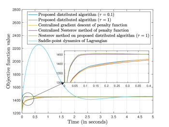
Figure 1: Evolution of the objective function value under the proposed distributed dynamics with $\tau=10^{-1}$ and $1$, resp., the centralized gradient descent, the centralized and the distributed (using the proposed approach with $\tau=1$) Nesterov’s accelerated gradient method of the penalty function, and the saddle-point dynamics of the Lagrangian.

One can observe that the proposed distributed algorithm performs much better than the saddle-point dynamics. As expected, centralized Nesterov’s accelerated gradient method performs the best, followed by the distributed Nesterov method obtained by applying the acceleration to our proposed distributed algorithm. The output of the distributed algorithm for both values of $\tau$ is also close to that of the centralized gradient descent. Figure 2 show the evolution of the value of $Ax-C$ for the proposed distributed algorithm with $\tau=1$ and the saddle-point dynamics. Even though Proposition II.3 states that, for the centralized gradient descent counterpart, there is no guarantee of staying inside the feasible set for general constraints, Figure 2 shows that the distributed algorithm satisfies the constraints much better during the evolution than the saddle-point dynamics.

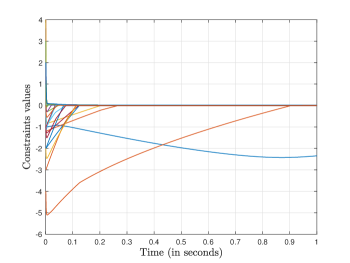
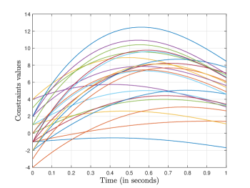
Figure 2: Evolution of the constraints under (a) the proposed distributed dynamics with $\tau=1$ and (b) the saddle-point dynamics.

In the next simulation we illustrate the robustness of the proposed dynamics. For this, we add a disturbance to the dynamics (26) using random vectors at each iteration as follows. For (26a), we add $d=\beta\|u(x,\Upsilon)\|\times(\text{unit-norm random vector})$, where we use the MATLAB function rand to generate random numbers between 0 and 1. Similarly, for (26b), we add $d=\beta\|w(x,\mathcal{P}_{\chi}\Upsilon)\|\times(\text{unit-norm random vector})$. For the scaling constant $\beta$, which also equals the ratio of the norm of the total disturbance to the norm of the unperturbed dynamics, we use gradually increasing values between 0.1 to 0.5. For each value of $\beta$, we plot the evolution of the objective function with $\tau=1$ in Figure 3. The plot shows the graceful degradation of the performance as the ratio of the norm of disturbance to the norm of unperturbed dynamics increases, demonstrating the effectiveness of the proposed dynamics against disturbances.

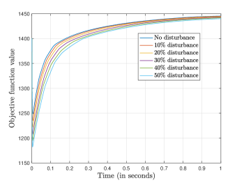
Figure 3: Evolution of the objective function value under the proposed distributed dynamics with $\tau=1$ in the presence of disturbances. The amount of disturbance in percentage denotes the ratio of the norm of the disturbance to the norm of the unperturbed dynamics.

VIII Conclusions

We have considered the problem of distributed optimization of a separable function under locally coupled constraints by a group of agents. Our approach relies on the reformulation of the optimization problem via a continuously differentiable exact penalty function. To enable the distributed computation of the gradient of this function, we have developed a distributed algorithm, of independent interest, to solve linear algebraic equations defined by separable data. This algorithm has exponential rate of convergence, is input-to-state stable, and does not require the individual agent matrices to be invertible. Building on this, we have introduced dynamics to asymptotically compute the gradient of the penalty function in a distributed fashion. Our algorithmic solution for optimization consists of implementing gradient descent and Nesterov’s accelerated method with the running estimates provided by this dynamics. We have shown the effectiveness of the proposed algorithm in simulation and compared its performance against a variety of other methods. Future work will explore the design of distributed algorithms for finding the least-square solutions of linear equations defined by separable problem data which only rely on 1-hop communication, distributed ways to determine the timescale of the estimation dynamics necessary to guarantee convergence, the characterization of the rate of convergence of the accelerated implementation, the study of constraint satisfaction along the executions, and the extension of our approach to problems involving global, non-sparse constraints.

Proof of Proposition II.3. To prove the result, we examine the Lie derivative of the constraint functions along the dynamics. We consider the different cases below:

(Equality constraints): Given the constraint function $h$, consider the Lie derivative over the set $\mathcal{F}$,

$$L_{-\nabla f^{\epsilon}}h(x) =-\nabla h(x)^{\prime}\big{(}\nabla f(x)+\nabla h(x)\mu(x)$$

$$\quad+\nabla\mu(x)h(x)+\frac{2}{\epsilon}\nabla h(x)h(x)\big{)}$$

$$=-\nabla h(x)^{\prime}(\nabla f(x)+\nabla h(x)\mu(x))$$

where we have used the fact that $h(x)=0$ for $x\in\mathcal{F}$. Substituting the value of $\mu(x)$ from (4),

$$L_{-\nabla f^{\epsilon}}h(x) =-\nabla h(x)^{\prime}(\nabla f(x)$$

$$\quad-\nabla h(x)N(x)^{-1}\nabla h(x)^{\prime}\nabla f(x))=0.$$

This means that the constraint function remains constant along the gradient dynamics over $\mathcal{F}$. Hence, $x(t)\in\mathcal{F}$ for all $t\geq t_{0}$ regardless of the value of $\epsilon$.

(Scalar inequality constraint): With only one inequality constraint defined by a scalar-valued function $g$, we have $x\in\mathcal{F}$ iff $g(x)\leq 0$. To determine the invariance of the feasibility set, we only need to look at points where $g(x)=0$. In this case, the Lie derivative is

$$L_{-\nabla f^{\epsilon}}g(x)=-\nabla g(x)^{\prime}\big{(}\nabla\lambda(x)+\frac{2}{\epsilon}\nabla g(x)\big{)}y^{\epsilon^{2}}(x),$$

where we have already used the fact that $g(x)=0$ and the definition of $\lambda(x)$ from (4). Due to LICQ assumption, $\nabla g(x)^{\prime}\nabla g(x)>0$, and $y^{\epsilon^{2}}(x)\geq 0$. Since $\nabla\lambda$ is continuous, it is bounded over the compact set $\mathcal{D}$. Hence, there exists $\bar{\epsilon}$ such that for all $\epsilon\in(0,\bar{\epsilon}]$, $L_{-\nabla f^{\epsilon}}g(x)\leq 0$ for all $x$ such that $g(x)=0$. This means that $x(t)\!\in\!\mathcal{F}$ for all $t\geq t_{0}$.

(General constraints): Here we provide a counterexample for the case with multiple inequality constraints (a similar one can be constructed for the case of both equality and inequality constraints). Consider now a vector-valued function $g$. The expression of the Lie derivative evaluated at $x$ such that $g(x)=0$ is

$$L_{-\nabla f^{\epsilon}}g=-\nabla g(x)^{\prime}\Big{(}\nabla\lambda(x)+\frac{2}{\epsilon}\nabla g(x)\Big{)}Y^{\epsilon}(x)y^{\epsilon}(x).$$

The LICQ assumption implies that $\nabla g(x)^{\prime}\nabla g(x)$ is positive definite. However, in general, this is not sufficient to ensure that the trajectory of the gradient dynamics starting from $x$ will remain in $\mathcal{F}$. To see this, consider the following example.

$$\min_{x} (x_{1}-1)^{2}+(x_{2}+1)^{2}$$

  s.t. $$x_{1}-6x_{2}\leq 0$$

$$-x_{1}+x_{2}\leq 0$$

Take $x=(0;0)$, where $g(x)=0$. After some calculations, it can be verified that $\lambda(x)=(0;-2)$ and $Y^{\epsilon}(x)y^{\epsilon}(x)=(0;\epsilon)$. As a result, $\nabla g(x)^{\prime}\nabla g(x)Y^{\epsilon}(x)y^{\epsilon}(x)=(-7\epsilon;2\epsilon)$ and $L_{-\nabla f^{\epsilon}}g=(14;2\epsilon-4)$. The first component of $L_{-\nabla f^{\epsilon}}g$ is independent of $\epsilon$. This means that no matter what value of $\epsilon$ we choose, $L_{-\nabla f^{\epsilon}}g\nleq 0$ when $g(x)=0$. Hence, the feasible set is not invariant. $\hfill\blacksquare$

Priyank Srivastava received the B.Tech degree in electrical engineering from National Institute of Technology, Kurukshetra, India in 2012, and the M.Tech degree in control & automation from Indian Institute of Technology Delhi, India in 2016. He is currently pursuing Ph.D. in mechanical engineering at the University of California San Diego, USA. His current research interests include dynamical systems, distributed and fast optimization, and coordination of distributed energy resources to enable their participation in energy markets.

Jorge Cortés (M’02, SM’06, F’14) received the Licenciatura degree in mathematics from Universidad de Zaragoza, Zaragoza, Spain, in 1997, and the Ph.D. degree in engineering mathematics from Universidad Carlos III de Madrid, Madrid, Spain, in 2001. He held postdoctoral positions with the University of Twente, Twente, The Netherlands, and the University of Illinois at Urbana-Champaign, Urbana, IL, USA. He was an Assistant Professor with the Department of Applied Mathematics and Statistics, University of California, Santa Cruz, CA, USA, from 2004 to 2007. He is currently a Professor in the Department of Mechanical and Aerospace Engineering, University of California, San Diego, CA, USA. He is the author of Geometric, Control and Numerical Aspects of Nonholonomic Systems (Springer-Verlag, 2002) and co-author (together with F. Bullo and S. Martínez) of Distributed Control of Robotic Networks (Princeton University Press, 2009). He is a Fellow of IEEE and SIAM. At the IEEE Control Systems Society, he has been a Distinguished Lecturer (2010-2014), and is currently its Director of Operations and an elected member (2018-2020) of its Board of Governors. His current research interests include distributed control and optimization, network science, resource-aware control, nonsmooth analysis, reasoning and decision making under uncertainty, network neuroscience, and multi-agent coordination in robotic, power, and transportation networks.

References

- [1] P. Srivastava and J. Cortés, “Distributed algorithm via continuously differentiable exact penalty method for network optimization,” in IEEE Conf. on Decision and Control, Miami Beach, FL, Dec. 2018, pp. 975–980.
- [2] D. P. Bertsekas and J. N. Tsitsiklis, Parallel and Distributed Computation: Numerical Methods. Athena Scientific, 1997.
- [3] M. G. Rabbat and R. D. Nowak, “Quantized incremental algorithms for distributed optimization,” IEEE Journal on Selected Areas in Communications, vol. 23, no. 4, pp. 798–808, 2005.
- [4] P. Wan and M. D. Lemmon, “Event-triggered distributed optimization in sensor networks,” in Symposium on Information Processing of Sensor Networks, San Francisco, CA, 2009, pp. 49–60.
- [5] A. Nedić, “Distributed optimization,” in Encyclopedia of Systems and Control, J. Baillieul and T. Samad, Eds. New York: Springer, 2015.
- [6] D. Feijer and F. Paganini, “Stability of primal-dual gradient dynamics and applications to network optimization,” Automatica, vol. 46, pp. 1974–1981, 2010.
- [7] D. Richert and J. Cortés, “Robust distributed linear programming,” IEEE Transactions on Automatic Control, vol. 60, no. 10, pp. 2567–2582, 2015.
- [8] E. Mallada, C. Zhao, and S. H. Low, “Optimal load-side control for frequency regulation in smart grids,” IEEE Transactions on Automatic Control, vol. 62, no. 12, pp. 6294–6309, 2017.
- [9] S. Boyd, N. Parikh, E. Chu, B. Peleato, and J. Eckstein, “Distributed optimization and statistical learning via the alternating direction method of multipliers,” Foundations and Trends in Machine Learning, vol. 3, no. 1, pp. 1–122, 2011.
- [10] Y. Xu, T. Han, K. Cai, Z. Lin, G. Yan, and M. Fu, “A distributed algorithm for resource allocation over dynamic digraphs,” IEEE Transactions on Signal Processing, vol. 65, no. 10, pp. 2600–2612, 2017.
- [11] S. A. Alghunaim, K. Yuan, and A. H. Sayed, “A proximal diffusion strategy for multi-agent optimization with sparse affine constraints,” IEEE Transactions on Automatic Control, 2020, to appear.
- [12] L. Xiao and S. Boyd, “Optimal scaling of a gradient method for distributed resource allocation,” Journal of Optimization Theory & Applications, vol. 129, no. 3, pp. 469–488, 2006.
- [13] B. Johansson and M. Johansson, “Distributed non-smooth resource allocation over a network,” in IEEE Conf. on Decision and Control, Shanghai, China, Dec. 2009, pp. 1678–1683.
- [14] A. Cherukuri and J. Cortés, “Distributed generator coordination for initialization and anytime optimization in economic dispatch,” IEEE Transactions on Control of Network Systems, vol. 2, no. 3, pp. 226–237, 2015.
- [15] T. Glad and E. Polak, “A multiplier method with automatic limitation of penalty growth,” Mathematical Programming, vol. 17, no. 1, pp. 140–155, 1979.
- [16] G. Di Pillo and L. Grippo, “Exact penalty functions in constrained optimization,” SIAM Journal on Control and Optimization, vol. 27, no. 6, pp. 1333–1360, 1989.
- [17] S. Lucidi, “New results on a continuously differentiable exact penalty function,” SIAM Journal on Optimization, vol. 2, no. 4, pp. 558–574, 1992.
- [18] G. Di Pillo, “Exact penalty methods,” in Algorithms for Continuous Optimization: The State of the Art, E. Spedicato, Ed. Dordrecht, The Netherlands: Kluwer Academic Publishers, 1994, pp. 209–253.
- [19] P. Srivastava and J. Cortés, “Nesterov acceleration for equality-constrained convex optimization via continuously differentiable penalty functions,” IEEE Control Systems Letters, vol. 5, no. 2, pp. 415–420, 2021.
- [20] C. D. Godsil and G. F. Royle, Algebraic Graph Theory, ser. Graduate Texts in Mathematics. Springer, 2001, vol. 207.
- [21] D. P. Bertsekas, Nonlinear Programming, 2nd ed. Belmont, MA: Athena Scientific, 1999.
- [22] R. T. Rockafellar, “Augmented Lagrange multiplier functions and duality in nonconvex programming,” SIAM Journal on Control, vol. 12, no. 2, pp. 268–285, 1974.
- [23] E. Dall’Anese, H. Zhu, and G. B. Giannakis, “Distributed optimal power flow for smart microgrids,” IEEE Transactions on Smart Grid, vol. 4, no. 3, pp. 1464–1475, 2013.
- [24] F. P. Kelly, A. K. Maulloo, and D. K. H. Tan, “Rate control in communication networks: Shadow prices, proportional fairness and stability,” Journal of the Operational Research Society, vol. 49, no. 3, pp. 237–252, 1998.
- [25] Q. Ba, K. Savla, and G. Como, “Distributed optimal equilibrium selection for traffic flow over networks,” in IEEE Conf. on Decision and Control, Osaka, Japan, 2015, pp. 6942–6947.
- [26] K. Arrow, L. Hurwitz, and H. Uzawa, Studies in Linear and Non-Linear Programming. Stanford, CA: Stanford University Press, 1958.
- [27] A. Cherukuri, B. Gharesifard, and J. Cortés, “Saddle-point dynamics: conditions for asymptotic stability of saddle points,” SIAM Journal on Control and Optimization, vol. 55, no. 1, pp. 486–511, 2017.
- [28] Y. E. Nesterov, “A method of solving a convex programming problem with convergence rate ,” Soviet Mathematics Doklady, vol. 27, no. 2, pp. 372–376, 1983.
- [29] D. P. Bertsekas, Constrained Optimization and Lagrange Multiplier Methods. Belmont, MA: Athena Scientific, 1982.
- [30] J. F. C. Mota, J. M. F. Xavier, P. M. Q. Aguiar, and M. Püschel, “D-ADMM: A communication-efficient distributed algorithm for separable optimization,” IEEE Transactions on Signal Processing, vol. 61, no. 10, pp. 2718–2723, 2013.
- [31] H. K. Khalil, Nonlinear Systems, 3rd ed. Prentice Hall, 2002.
- [32] S. Mou, J. Liu, and A. S. Morse, “A distributed algorithm for solving a linear algebraic equation,” IEEE Transactions on Automatic Control, vol. 60, no. 11, pp. 2863–2878, 2015.
- [33] B. D. O. Anderson, S. Mou, A. S. Morse, and U. Helmke, “Decentralized gradient algorithm for solution of a linear equation,” Numerical Algebra, Control and Optimization, vol. 6, no. 3, pp. 319–328, 2016.
- [34] J. Lu and C. Y. Tang, “A distributed algorithm for solving positive definite linear equations over networks with membership dynamics,” IEEE Transactions on Control of Network Systems, vol. 5, no. 1, pp. 215–227, 2018.
- [35] D. P. Spanos, R. Olfati-Saber, and R. M. Murray, “Distributed sensor fusion using dynamic consensus,” in IFAC World Congress, Prague, CZ, Jul. 2005, electronic proceedings.
- [36] L. Xiao, S. Boyd, and S. Lall, “A scheme for robust distributed sensor fusion based on average consensus,” in Symposium on Information Processing of Sensor Networks, Los Angeles, CA, Apr. 2005, pp. 63–70.
- [37] X. Wang and S. Mou, “A distributed algorithm for achieving the conservation principle,” in American Control Conference, Milwaukee, WI, June 2018, pp. 5863–5867.
- [38] V. Veliov, “A generalization of the Tikhonov theorem for singularly perturbed differential inclusions,” Journal of Dynamical & Control Systems, vol. 3, no. 3, pp. 291–319, 1997.
- [39] J. Rivera and H. Jacobsen, “A distributed anytime algorithm for network utility maximization with application to real-time EV charging control,” in IEEE Conf. on Decision and Control, Los Angeles, CA, Dec. 2014, pp. 947–952.
- [40] A. U. Raghunathan and S. Krishnamurthy, “A distributed anytime algorithm for maximizing occupant comfort,” in American Control Conference, Montreal, Canada, Jun. 2012, pp. 1059–1066.