MLAS: Metric Learning on Attributed Sequences

Abstract

Distance metric learning has attracted much attention in recent years, where the goal is to learn a distance metric based on user feedback. Conventional approaches to metric learning mainly focus on learning the Mahalanobis distance metric on data attributes. Recent research on metric learning has been extended to sequential data, where we only have structural information in the sequences, but no attribute is available. However, real-world applications often involve attributed sequence data (e.g., clickstreams), where each instance consists of not only a set of attributes (e.g., user session context) but also a sequence of categorical items (e.g., user actions). In this paper, we study the problem of metric learning on attributed sequences. Unlike previous work on metric learning, we now need to go beyond the Mahalanobis distance metric in the attribute feature space while also incorporating the structural information in sequences. We propose a deep learning framework, called MLAS (Metric Learning on Attributed Sequences), to learn a distance metric that effectively measures dissimilarities between attributed sequences. Empirical results on real-world datasets demonstrate that the proposed MLAS framework significantly improves the performance of metric learning compared to state-of-the-art methods on attributed sequences.

I Introduction

Distance metric learning, where the goal is to learn a distance metric based on a set of similar/dissimilar pairs of instances, has attracted significant attention in recent years [1, 2, 3, 4, 5, 6]. Many real-world applications from web log analysis to user profiling could significantly benefit from distance metric learning.

Conventional approaches to distance metric learning [7, 8, 4, 9] focus on learning a Mahalanobis distance metric, which is equivalent to learning a linear transformation on data attributes. Recent research has extended distance metric learning to nonlinear settings using deep neural networks [10, 5], where a nonlinear mapping function is first learned to project the instances into a new space, and then the final metric becomes the Euclidean distance metric in that space. With the flexibility and powerfulness demonstrated in various applications, distance metric learning using neural networks has been the method of choice for learning such nonlinear mappings [11, 12, 10, 5, 6].

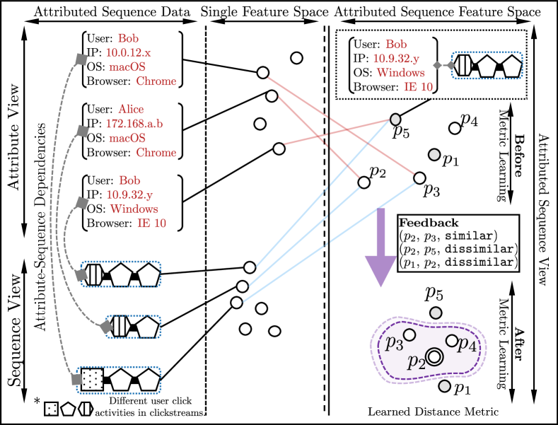
Figure 1: Metric learning on attributed sequences.

While some recent research on metric learning has begun to explore more complex data, such as sequences [6], web applications often involve the even more complex attributed sequence, where each instance consists of not only a sequence of categorical items but also a set of attributes of numerical or categorical values. For example, each user browsing session in a bot detection system can be viewed as an attributed sequence, with the series of click activities as the sequence and static context (e.g., browser name, operating system version) as the attributes. Furthermore, the attributes and the sequences from the many applications are not independent of each other. For example, in a web search, each user session is composed of a session profile modeled by a set of attributes (e.g., type of device, operating system, etc) as well as a sequence of search keywords. One keyword may depend on previous search terms (e.g., “temperature” following “snow storm”) and the keywords searched may also depend on the attribute device type (e.g., “nearest restaurant” on “cellphone”).

In this paper, we study this new problem of distance metric learning on attributed sequences, where the distance between similar attributed sequences is minimized, while dissimilar ones become well-separated with a margin. This problem is core to many applications from fraud detection to user behavior analysis for targeted advertising. This problem is challenging since explicit class labels for attributed sequences are often not available. Instead, only a few pairs of attributed sequences may be known to be similar or dissimilar. This problem differs from previous works on metric learning [7, 2, 3] because we need to go beyond linear transformations in the attribute feature space while incorporating not only the structural information in sequences but also the dependencies between attributes and sequences. In this work, we propose a deep learning framework, called MLAS (Metric Learning on Attributed Sequences), targeting at learning a distance metric that can effectively exploit the similarity and dissimilarity between each pair of attributed sequences. Our paper offers the following contributions:

• We formulate and study the problem of distance metric learning on attributed sequences.

• We design three main sub-networks to learn the information from the attributes, the sequences, and the attribute-sequence dependencies.

• We design three distinct integrated deep learning architectures with three main sub-networks.

• We design an experimental strategy to evaluate and compare the distance metric learned by our proposed MLAS network with various baseline methods.

We organize the paper as follows. We first define our problem in Section II. We detail the MLAS network design and the metric learning process in Section III. Next, we present the experimental methodology and results in Section IV. We summarize the related work in Section V. We conclude our findings and discuss future research directions in Section VI.

II Problem Formulation

II-A Preliminaries

Definition 1 (Sequence)

Given a set of categorical items $\mathcal{I}=\{e_{1},\cdots,e_{r}\}$, a sequence $S_{k}=\left(\alpha_{k}^{(1)},\cdots,\alpha_{k}^{(T_{k})}\right)$ is an ordered list of $T_{k}$ items, where the item at $t$-th time step $\alpha_{k}^{(t)}\in\mathcal{I},\forall t=1,\cdots,T_{k}$.

In prior work [13], one common preprocessing step is to zero-pad each sequence to the longest sequence in the dataset and then to one-hot encode it. Without loss of generality, we denote the length of the longest sequence as $T$. For each $k$-th sequence $S_{k}$ in the dataset, we denote its equivalent one-hot encoded sequence as: $\mathbf{S}_{k}=\left(\bm{\alpha}_{k}^{(1)},\cdots,\bm{\alpha}_{k}^{(T)}\right)$, where $\bm{\alpha}_{k}^{(t)}\in\mathbb{R}^{r}$ corresponds to a vector represents the item $\alpha_{k}^{(t)}$ with the $l$-th entry in $\bm{\alpha}_{k}^{(t)}$ is “1” and all other entries are zeros if $\alpha_{k}^{(t)}=e_{l},e_{l}\in\mathcal{I}$.

Definition 2 (Attributed Sequence)

Given an attribute vector $\mathbf{x}_{k}\in\mathbb{R}^{u}$ with $u$ attributes, and a sequence $\mathbf{S}_{k}\in\mathbb{R}^{T\times r}$, an attributed sequence $p_{k}=(\mathbf{x}_{k},\mathbf{S}_{k})\in\left(\mathbb{R}^{u},\mathbb{R}^{T\times r}\right)$ is a pair composed of the attribute vector $\mathbf{x}_{k}$ and the corresponding sequence $\mathbf{S}_{k}$.

For example, in a flight booking system, one attributed sequence represents a booking session by the end user. In this case, the attribute vector represents the booking session’s profile (e.g., IP address, session duration, etc) while the sequence consists of the end user’s activities on the booking webpage. Given a set of $n$ attributed sequences $\mathcal{J}=\{J_{1},\cdots,J_{n}\}$, $\mathbf{S}_{k}\in\mathbb{R}^{T\times r}$, where $T=\max\{T_{1},\cdots,T_{n}\}$. Each attribute vector is composed of a number of attributes, where the value of each attribute is in $\mathbb{R}$. The dimension of attribute value vectors depends on the number of distinct attribute value combinations.

We further define the feedback as a collection of similar (or dissimilar) attributed sequence pairs.

Definition 3 (Feedback)

Let $\mathcal{P}=\{p_{1},\cdots,p_{n}\}$ be a set of $n$ attributed sequences. A feedback is a triplet $(p_{i},p_{j},\ell_{ij})$ consisting of two attributed sequences $p_{i},p_{j}\in\mathcal{P}$ and a label $\ell_{ij}\in\{0,1\}$ indicating whether $p_{i}$ and $p_{j}$ are similar ($\ell_{ij}=0$) or dissimilar ($\ell_{ij}=1$). We define a similar feedback set $\mathcal{S}=\{(p_{i},p_{j},\ell_{ij})|\ell_{ij}=0\}$ and a dissimilar feedback set $\mathcal{D}=\{(p_{i},p_{j},\ell_{ij})|\ell_{ij}=1\}$.

The feedback could be given by domain experts in real-world applications based on their domain experiences.

An Example of Feedback. In a user behavior analysis application, each user visit is depicted as an attributed sequence. Given two user sessions $p_{1}$ and $p_{2}$, domain experts may imply they are similar by giving the feedback $(p_{1},p_{2},0)$; or imply they are dissimilar by the feedback $(p_{1},p_{2},1)$.

II-B Problem definition

Given a nonlinear transformation function $\Theta$ and two attributed sequences $p_{i}$ and $p_{j}$ as inputs, deep metric learning approaches [5] often apply the Mahalanobis distance function to the $d$-dimensional outputs of function $\Theta$ as:

$$D_{\Theta}(p_{i},p_{j})=\sqrt{(\Theta(p_{i})-\Theta(p_{j}))^{\top}\boldsymbol{\Lambda}(\Theta(p_{i})-\Theta(p_{j}))}$$ (1)

where $\boldsymbol{\Lambda}\in\mathbb{R}^{d\times d}$ is a symmetric, semi-definite, and positive matrix. When $\boldsymbol{\Lambda}=\mathbf{I}$, Equation 1 is equivalent to Euclidean distance [7] as:

$$D_{\Theta}(p_{i},p_{j})=\|\Theta(p_{i})-\Theta(p_{j})\|_{2}.$$ (2)

Given feedback sets $\mathcal{S}$ and $\mathcal{D}$ of attributed sequences as per Def. 3 and a distance function $D_{\Theta}$ as per Equation 2, the goal of deep metric learning on attributed sequences is to find the transformation function $\Theta:(\mathbb{R}^{u},\mathbb{R}^{T\times r})\mapsto\mathbb{R}^{d}$ with a set of parameters $\theta$ that is capable of mapping the attributed sequence inputs to a space that the distances between each pair of attributed sequences in the similar feedback set $\mathcal{S}$ are minimized while increasing the distances between attributed sequence pairs in the dissimilar feedback set $\mathcal{D}$. Inspired by [7], we adopt the learning objective as:

$$\begin{split}\operatorname*{minimize}_{\theta}&\sum_{(p_{i},p_{j},\ell_{ij})\in\mathcal{S}}D_{\Theta}\left(p_{i},p_{j}\right)\\[2.0pt] \textrm{s.t.}&\sum_{(p_{i},p_{j},\ell_{ij})\in\mathcal{D}}D_{\Theta}\left(p_{i},p_{j}\right)\geq g\\ \end{split}$$ (3)

where $g$ is a group-based margin parameter that stipulates the distance between two attributed sequences from dissimilar feedback set should be larger than $g$. This prevents the dataset from being reduced to a single point [7].

III The MLAS Network Architecture

We first design two networks to handle attributed sequence data. Namely, the AttNet using feedforward fully connected neural networks for the attributes and the SeqNet using long short-term memory (LSTM) for the sequences. Next, we explore three design variations of the FusionNet concerning the attribute-sequence dependencies. Lastly, the FusionNet is augmented by MetricNet to exploit the user feedback.

III-A AttNet and SeqNet Design

III-A1 AttNet

AttNet is designed using a fully connected neural network to learn the relationships within attribute data. In particular, for an AttNet with $M$ layers, we denote the weight and bias parameters of the $m$-th layer as $\mathbf{W}_{A}^{(m)}$ and $\mathbf{b}_{A}^{(m)},\forall m=1,\cdots,M$. Given an attribute vector $\mathbf{x}_{k}\in\mathbb{R}^{u}$ as the input, with $d_{m}$ hidden units in the $m$-th layer of AttNet, the corresponding output is $\mathbf{V}^{(m)}\in\mathbb{R}^{d_{m}},\forall m=1,\cdots,M$. Note that the choice of $M$ is task-specific. Although neural networks with more layers are better at learning hierarchical structure in the data, it is also observed that such networks are difficult to train due to the multiple nonlinear mappings that prevent the information and gradient passing along the computation graph [14]. The AttNet is designed as:

$$\small\begin{split}\mathbf{V}^{(1)}&=\delta\left(\mathbf{W}_{A}^{(1)}\mathbf{x}_{k}+\mathbf{b}_{A}^{(1)}\right)\\[-6.0pt] \vdots\\[-3.0pt] \mathbf{V}^{(M)}&=\delta\left(\mathbf{W}_{A}^{(M)}\mathbf{V}^{(M-1)}+\mathbf{b}_{A}^{(M)}\right)\end{split}$$ (4)

where $\delta:\mathbb{R}^{d_{m}}\mapsto\mathbb{R}^{d_{m}}$ is a hyperbolic tangent activation function.

Given the attribute vector $\mathbf{x}_{k}\in\mathbb{R}^{u}$ as the input, the first layer of AttNet uses the weight matrix $\mathbf{W}_{A}^{(1)}\in\mathbb{R}^{d_{1}\times u}$ and bias vector $\mathbf{b}_{A}^{(1)}\in\mathbb{R}^{d_{1}}$ to map $\mathbf{x}_{k}$ to the output $\mathbf{V}^{(1)}\in\mathbb{R}^{d_{1}}$ with $d_{1}<u$. The $\mathbf{V}^{(1)}$ is subsequently used as the input to the next layer. We denote the AttNet as $\Theta_{A}:\mathbb{R}^{u}\mapsto\mathbb{R}^{d_{M}}$, where $\Theta_{A}$ is parameterized by $\mathbf{W}_{A}$ and $\mathbf{b}_{A}$, where $\mathbf{W}_{A}=\left[\mathbf{W}_{A}^{(1)},\cdots,\mathbf{W}_{A}^{(M)}\right]$ and $\mathbf{b}_{A}=\left[\mathbf{b}_{A}^{(1)},\cdots,\mathbf{b}_{A}^{(M)}\right]$.

III-A2 SeqNet

The SeqNet is designed to learn the dependencies between items in the input sequences by taking advantage of the long short-term memory (LSTM) [15] network to learn the dependencies within the sequences.

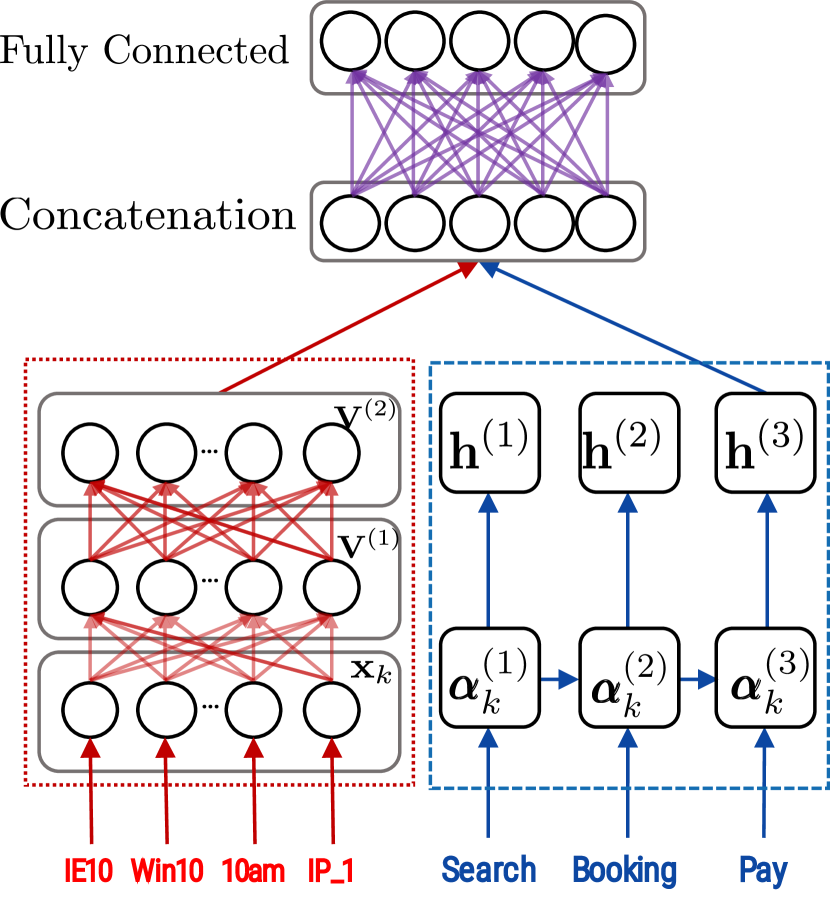
(a) Balanced Design

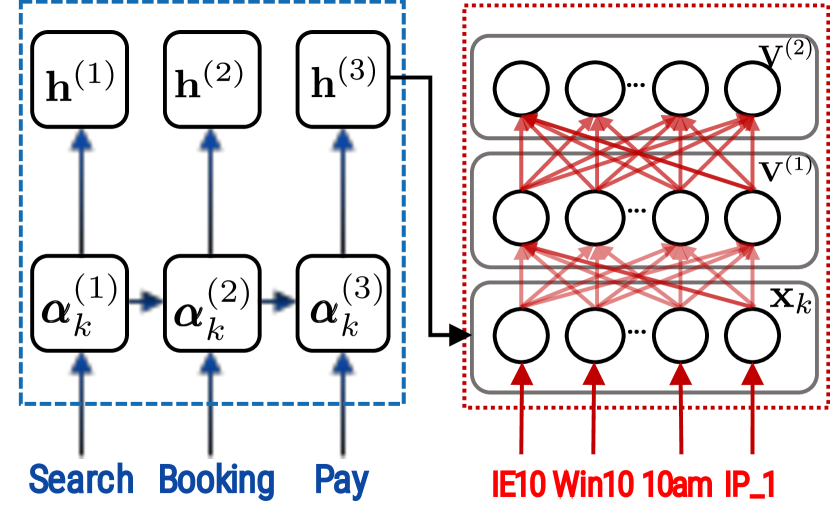
(b) AttNet-centric Design

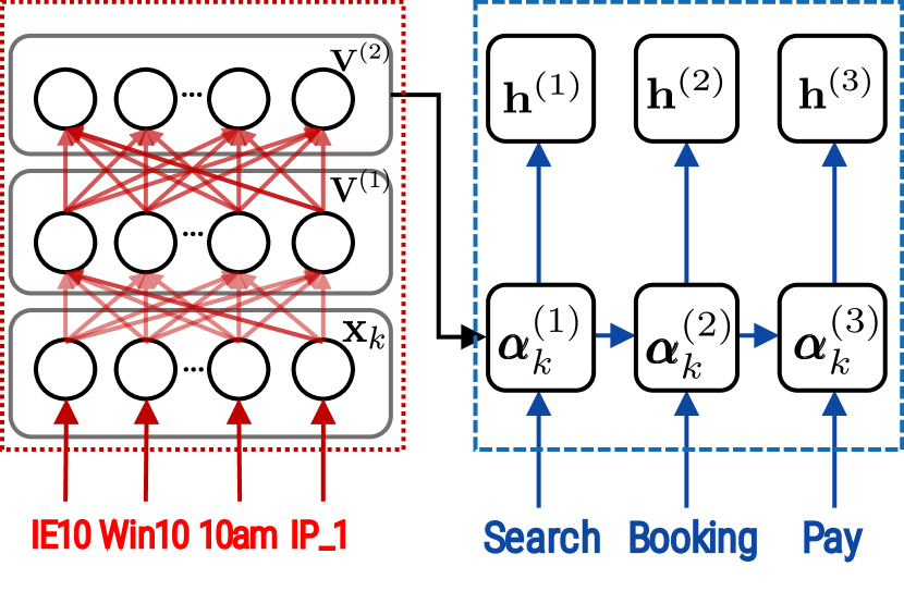
(c) SeqNet-centric Design

Figure 2: Three different FusionNet designs.

Given a sequence input $\mathbf{S}_{k}\in\mathbb{R}^{T\times r}$, we have the parameters within SeqNet at time step $t$ as:

$$\begin{split}\mathbf{i}^{(t)}&=\sigma\left(\mathbf{W}_{i}\bm{\alpha}_{k}^{(t)}+\mathbf{U}_{i}\mathbf{h}^{(t-1)}+\mathbf{b}_{i}\right)\\[-2.0pt] \mathbf{f}^{(t)}&=\sigma\left(\mathbf{W}_{f}\bm{\alpha}_{k}^{(t)}+\mathbf{U}_{f}\mathbf{h}^{(t-1)}+\mathbf{b}_{f}\right)\\[-2.0pt] \mathbf{o}^{(t)}&=\sigma\left(\mathbf{W}_{o}\bm{\alpha}_{k}^{(t)}+\mathbf{U}_{o}\mathbf{h}^{(t-1)}+\mathbf{b}_{o}\right)\\[-2.0pt] \mathbf{g}^{(t)}&=\tanh\left(\mathbf{W}_{c}\bm{\alpha}_{k}^{(t)}+\mathbf{U}_{c}\mathbf{h}^{(t-1)}+\mathbf{b}_{c}\right)\\[-2.0pt] \mathbf{c}^{(t)}&=\mathbf{f}^{(t)}\odot\mathbf{c}^{(t-1)}+\mathbf{i}^{(t)}\odot\mathbf{g}^{(t)}\\[-2.0pt] \mathbf{h}^{(t)}&=\mathbf{o}^{(t)}\odot\tanh\left(\mathbf{c}^{(t)}\right)\end{split}$$ (5)

where $\sigma(z)=\frac{1}{1+e^{-z}}$ is a logistic activation function, $\odot$ denotes the bitwise multiplication, $\mathbf{i}^{(t)}$, $\mathbf{f}^{(t)}$ and $\mathbf{o}^{(t)}$ are the internal gates of the LSTM, $\mathbf{c}^{(t)}$ and $\mathbf{h}^{(t)}$ are the cell and hidden states of the LSTM. For simplicity, we denote the SeqNet with $d_{S}$ hidden units as $\Theta_{S}:\mathbb{R}^{T\times r}\mapsto\mathbb{R}^{d_{S}}$, where $\Theta_{S}$ is parameterized by bias vector set $\mathbf{b}_{S}=\left[\mathbf{b}_{i},\mathbf{b}_{f},\mathbf{b}_{o},\mathbf{b}_{c}\right]$ and the weight matrices $\mathbf{W}_{S}\!=\!\left[\mathbf{W}_{i},\mathbf{W}_{f},\mathbf{W}_{o},\mathbf{W}_{c}\right]\in\mathbb{R}^{4\times d_{S}\times r}$ and recurrent matrices $\mathbf{U}_{S}=\left[\mathbf{U}_{i},\mathbf{U}_{f},\mathbf{U}_{o},\mathbf{U}_{c}\right]\in\mathbb{R}^{4\times d_{S}\times d_{S}}$.

III-B FusionNet Design

One important design in MLAS is the FusionNet (denoted as $\Theta$), where the AttNet and SeqNet are connected together with the goal of producing feature representation outputs for the attributed sequences. Based on the possible ways of connecting the AttNet and the SeqNet, we propose three FusionNet design variations: (1) balanced, (2) AttNet-centric and (3) SeqNet-centric. We evaluate the performance of all three variations in Section IV.

III-B1 Balanced Design (Figure 2(a)).

The AttNet and SeqNet are concatenated together and augmented by an additional layer fully connected neural network. This additional layer of fully connected neural network is used to capture the dependencies between the attributes and the sequences. For each attributed sequence, we only use the output of SeqNet after the last time step of the sequence has been processed to capture the complete information of the sequence. We denote the balanced design as:

$$\normalsize\mathbf{y} =\mathbf{V}^{(M)}\oplus\mathbf{h}^{(T_{k})}$$

$$\mathbf{z} =\delta\left(\mathbf{W}_{z}\mathbf{y}+\mathbf{b}_{z}\right)$$

where $\oplus$ represents the concatenation operation, $\mathbf{W}_{z}\in\mathbb{R}^{d\times(d_{M}+d_{S})}$ and $\mathbf{b}_{z}\in\mathbb{R}^{d}$ denote the weight matrix and bias vector in this fully connected layer, respectively.

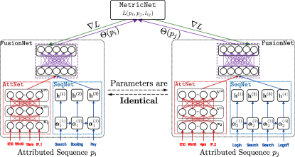
Figure 3: MLAS network with balanced design. Parameters in the two FusionNet are shared. The feature representations are used by MetricNet to compute the loss $L$. The gradient $\nabla L$ is used to update all layers.

III-B2 AttNet-centric Design (Figure 2(b)).

Here, the sequence is first transformed by the sequence network, i.e., the function $\Theta_{S}$, and then used as an input of the AttNet. Specifically, we modify Equation 4 to incorporate sequence representation as input. Similar to the balanced design, only the output of SeqNet after processing the last time step of the sequence is used to capture the complete information. The modified $\mathbf{V}_{k}^{(1)}$ is written as:

$$\mathbf{V}^{(1)}=\delta\left(\mathbf{W}_{A}^{(1)}\left(\mathbf{x_{k}}\oplus\mathbf{h}^{(T_{k})}\right)+\mathbf{b}_{A}^{(1)}\right)$$

where the $\mathbf{W}_{A}^{(1)}\in\mathbb{R}^{d_{1}\times(u+d_{S})}$ and $\mathbf{b}_{A}^{(1)}\in\mathbb{R}^{d_{1}}$.

III-B3 SeqNet-centric Design (Figure 2(c)).

The output of AttNet is used as an additional input for SeqNet . Specifically, we modify Equation 5 to integrate attribute representations at the first time step. The modified $\mathbf{h}_{k}^{(t)}$ is defined as:

$$\mathbf{h}^{(1)}=\mathbf{o}^{(1)}\odot\tanh\left(\mathbf{c}^{(1)}\right)+\mathbf{V}^{(M)}$$

where $\odot$ denotes the bitwise multiplication. The SeqNet is conditioned using the information from AttNet.

III-C The MetricNet

We present the MetricNet using the proposed balanced design due to space limitations. In the balanced design (as shown in Figure 2(a)), the explicit form of FusionNet can be written as:

$$\Theta(p_{k})=\Theta_{A}\left(\Theta_{A}(\mathbf{x}_{k})\oplus\Theta_{S}(\mathbf{S}_{k})\right)$$ (6)

Given an attributed sequence feedback instance $(p_{i},p_{j},\ell_{ij})$, where $p_{i}=(\mathbf{x}_{i},\mathbf{S}_{i})$ and $p_{j}=(\mathbf{x}_{j},\mathbf{S}_{j})$, $\ell_{ij}\in\{1,0\}$. This input is transformed to $\Theta(p_{i})\in\mathbb{R}^{d}$ and $\Theta(p_{j})\in\mathbb{R}^{d}$ by the nonlinear transformation $\Theta$ of FusionNet at the first step.

Next, the two outputs of FusionNet are taken by the MetricNet to calculate the differences between them. The MetricNet is designed to utilize a contrastive loss function [16] so that attributed sequences in each similar pair in $\mathcal{S}$ have a smaller distance compared to those in $\mathcal{D}$ after learning the distance metric. The learning objective of MetricNet can be written as:

$$L(p_{i},p_{j},\ell_{ij})=\frac{1}{2}(1-\ell_{ij})(D_{\Theta})^{2}+\frac{1}{2}\ell_{ij}\{\max(0,g-D_{\Theta})\}^{2}$$ (7)

where $g$ is the margin parameter, meaning that the pairs with a dissimilar label ($\ell_{ij}=1$) contribute to the learning objective if and only if when the Euclidean distance between them is smaller than $g$ [16].

For each pair of FusionNet outputs, MetricNet first computes the Euclidean distance (Equation 2) between them. Then the contrastive loss is computed using both the Euclidean distance and the label. We note that the MetricNet can augment all three designs in the same way. Figure 3 illustrates the MetricNet with the proposed balanced design.

The parameters in both FusionNet and MetricNet are adjusted using the metric learning presented in Algorithm 1.

1:A set of attributed sequences $\mathcal{P}=\{p_{1},\cdots,p_{n}\}$, a set of feedback as pairwise attributed sequences $\mathcal{C}=\{(p_{i},p_{j},\ell_{ij})|p_{i},p_{j}\in\mathcal{P},\}$, the number of layers $M$, learning rate $\gamma$, number of iterations $\vartheta$ and convergence error $\epsilon$.

2:Parameter sets $\{\mathbf{W}_{A},\mathbf{b}_{A},\mathbf{W}_{S},\mathbf{U}_{S},\mathbf{b}_{S}\}$.

3:Initialize MLAS network $\Theta$.

4:Pre-train the MLAS network.

5:for each $\vartheta^{\prime}=1,\cdots,\vartheta$ do

6:     for each $(p_{i},p_{j},\ell_{ij})\in\mathcal{C}$ do

7:         //Forward propagation.

8:         Calculate $\Theta(p_{i})$ and $\Theta(p_{j})$.

9:         Calculate $D_{\Theta}$ using Equation 2.

10:         Calculate loss $L_{\vartheta^{\prime}}(p_{i},p_{j},\ell_{ij})$ (Equation 7).

11:         if $|L_{\vartheta^{\prime}}(p_{i},p_{j},\ell_{ij})-L_{\vartheta^{\prime}-1}(p_{i},p_{j},\ell_{ij})|<\epsilon$ then

12:              break

13:         end if

14:         //Back-propagation.

15:         Calculate $\frac{\partial L}{\partial\Theta}$.

16:         Calculate $\nabla L$.

17:         Update network parameters.

18:     end for

19:end for

Algorithm 1 Training the MLAS Network

IV Experiments

IV-A Datasets

We evaluate the proposed methods using four real-world datasets. Two of them are derived from application log files at Amadeus [17] (denoted as AMS-A and AMS-B). The other two datasets are derived from the Wikispeedia [18] dataset (denoted as Wiki-A and Wiki-B). For each dataset, we randomly sampled 80% as the training set and 20% as the testing set. The training and testing sets remain the same across all our experiments.

TABLE I: Summary of Compared Methods

Method	Data Used	Short Description	Reference
ATT	Attributes	Only attribute feedback is used in the model.	[5]
SEQ	Sequences	Only sequence feedback is used in the model.	[6]
ASF	Attributes Sequences	Feedback of attributes and sequences are used to train two models separatedly.	[5] + [6]
MLAS-B	Attributes Sequences Dependencies	Balanced design using attri- -buted sequence feedback to train one unified model.	This Work
MLAS-A	Attributes Sequences Dependencies	Attribute-centric design using attributed sequence feedback to train one unified model.	This Work
MLAS-S	Attributes Sequences Dependencies	Sequence-centric design using attributed sequence feedback to train one unified model.	This Work

• AMS-A: We used 58k user sessions from log files of an internal application from our Amadeus partner company. Each record has a user profile containing information ranging from system configurations to office name, and a sequence of functions invoked by click activities on the web interface. There are 288 distinct functions, 57,270 distinct user profiles in this dataset. The average length of the sequences is 18. We use 100 attributed sequence feedback pairs selected by the domain experts.

• AMS-B: There are 106k user sessions derived from application log files with 575 distinct functions and 106,671 distinct user profile. The average length of the sequences is 22. Domain experts select 84 attributed sequence feedback pairs.

• Wiki-A: This dataset is sampled from Wikispeedia dataset. Wikispeedia dataset originated from an online computation game [18], in which each user is given two pages (i.e., source, and destination) from a subset of Wikipedia pages and asked to navigate from the source to the destination page. We use a subset of $\sim$2k paths from Wikispeedia with the average length of the path as 6. We also extract 11 sequence context as attributes (e.g., the category of the source page, average time spent on each page, etc). There are 200 feedback instances selected based on the criteria of frequent subsequences and attribute value.

• Wiki-B: This dataset is also sampled from Wikispeedia dataset. We use a subset of $\sim$1.5k paths from Wikispeedia with the average length of the path as 8. We also extract 11 sequence context (e.g., the category of the source page, average time spent on each page, etc) as attributes. 220 feedback instances have been selected based on the criteria of frequent sub-sequences and attribute values.

IV-B Compared Methods

We validate the effectiveness of our proposed MLAS solution compared with state-of-the-art baseline methods. To well understand the advancements of the proposed methods, we use baselines that are working on only attributes (denoted as ATT) or sequences (denoted as SEQ), as well as methods without exploiting the dependencies between attributes and sequences (denoted as ASF) .

1. Attribute-only Feedback (ATT) [5]: Only attribute feedback is used in this model. This model first transforms fixed-size input data into feature vectors, then learns the similarities between these two inputs.

2. Sequence-only Feedback (SEQ) [6]: Only sequence feedback is used in this model. This model utilizes a long short-term memory (LSTM) to learn the similarities between two sequences.

3. Attribute and Sequence Feedback (ASF) [5] + [6]: This method is a combination of the ATT and SEQ methods as above, where the two networks are trained separately using attribute feedback and sequence feedback, respectively. The feature vectors generated by the two models are then concatenated.

4. Balanced Network Design with Attributed Sequence Feedback (MLAS-B): This is the balanced design model (Section III-B1) using attributed sequence feedback to train one unified model.

5. AttNet-centric Network Design with Attributed Sequence Feedback (MLAS-A): This is the AttNet-centric design (Section III-B2) using attributed sequence feedback to train one unified model.

6. SeqNet-centric Network Design with Attributed Sequence Feedback (MLAS-S): This is the SeqNet-centric design (Section III-B3) using attributed sequence feedback to train one unified model.

(a) AMS-A Dataset

(b) AMS-B Dataset

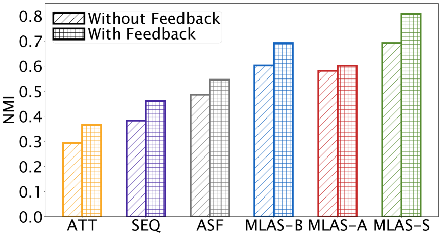
(c) Wiki-A Dataset

(d) Wiki-B Dataset

Figure 4: The effectiveness of using feedback. Using feedback could boost performance of all methods. The three methods we proposed (MLAS-B/A/S) are capable of exploiting the information of attributes, sequences, and more importantly, the attribute-sequence dependencies to outperform other methods.

(a) AMS-A Dataset

(b) AMS-B Dataset

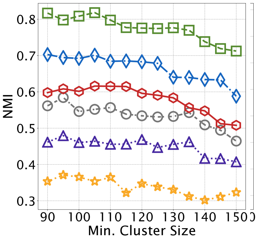
(c) Wiki-A Dataset

(d) Wiki-B Dataset

Figure 5: Performance with varying clustering parameters. Clustering results using the feature representations produced by MLAS are the best among the compared methods.

IV-C Experimental Settings

In this section, we present the settings for performance evaluation and parameter studies.

IV-C1 Network Initialization and Training

Initializing the network parameters is important for models using gradient descent based approaches [19]. The weight matrices $\mathbf{W}_{A}$ in $\Theta_{A}$ and the $\mathbf{W}_{S}$ in $\Theta_{S}$ are initialized using the uniform distribution [20], the biases $\mathbf{b}_{A}$ and $\mathbf{b}_{S}$ are initialized with zero vector $\boldsymbol{0}$ and the recurrent matrix $\mathbf{U}_{S}$ is initialized using orthogonal matrix [21]. We use one hidden layer ($M=1$) for AttNet and ATT in the experiments to make the training process easier.

After that, we pre-train each compared method. Pre-training is an important step to initialize the neural network-based models [19]. Our pre-training uses the attributed sequences as the inputs for FusionNet, and use the generated feature representations to reconstruct the attributed sequence inputs. We also pre-train the ATT and SEQ networks in a similar fashion that reconstruct the respective attributes or sequences. We utilize $\ell_{2}$-regularization and early stopping strategy to avoid overfitting. Twenty percents of feedback pairs are used in the validation set. We choose ReLU activation function [22] in our AttNet to accelerate the stochastic gradient descent convergence.

IV-C2 Performance Evaluation Setting.

We evaluate the performance by using the feature representations generated by each method for clustering tasks. The feature representations are generated through a forward pass.

Clustering tasks have been widely used in distance metric learning work [7, 1]. In this set of experiments, we use HDBSCAN [23] clustering algorithm. HDBSCAN is a deterministic algorithm, which gives identical output when using the same input. We measure the normalized mutual information (NMI) [24] score. The maximum NMI score is 1. Specifically, we conduct the below two experiments:

1. The effect of feedback. We compare the performance of the clustering algorithm using the feature representations generated by FusionNet before and after incorporating the feedback.

2. The effect of varying parameters in the clustering algorithm. After the metric learning process, we evaluate the feature representations generated by all compared methods under various parameters of the clustering algorithm.

IV-C3 Parameter Study Settings.

We evaluate the effect of output dimension (i.e., the dimension of the hidden layer), which affects the model size and the performance of downstream mining algorithms.

The other parameter we evaluate is the relative importance of attribute data (denoted as $\omega_{A}$) in the attributed sequences. The pre-training phase is essential to gradient descent-based methods [19]. The relative importance of attribute data and sequence data are represented by the weights of $\Theta_{A}$ and $\Theta_{S}$, denoted as $\omega_{A}$ and $\omega_{S}$, where $\omega_{A}+\omega_{S}=1$. The intuition is that with one data type more important, the other one becomes relatively less important.

IV-D Results and Analysis

IV-D1 Effect of Feedback.

We present the performance comparisons in clustering tasks using feature representations generated using the parameters of all methods in Figure 4. Two sets of feature representations are generated, the first set is generated after the pre-training (denoted as without feedback), the other set is generated after the metric learning step (denoted as with feedback). We fix the output dimension to 10, minimum cluster size to 100 and $\omega_{A}=0.5$ (for MLAS-B/A/S). We have observed that the feedback can boost the performance of all methods, and the three methods (MLAS-B/A/S) proposed in this work are capable of outperforming other methods. Also, we also observe that the proposed three MLAS variations have better performance compared to the ASF, which also uses the information from attributes and sequences but without using the attribute-sequence dependencies.

Based on the above observations, we can conclude that the performance boost of our three architectures (MLAS-B/A/S) is a result of taking advantages of attribute data, sequence data, and more importantly, the attribute-sequence dependencies.

(a) AMS-A Dataset

(b) AMS-B Dataset

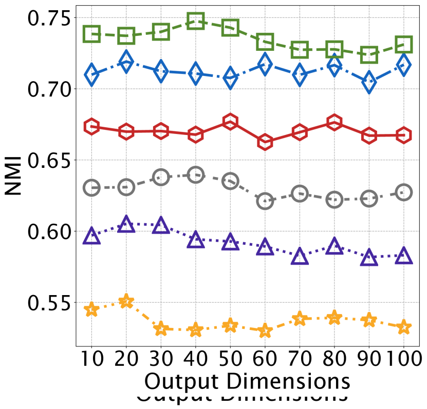
(c) Wiki-A Dataset

(d) Wiki-B Dataset

Figure 6: The effect of output dimensions (higher is better). Output dimension is an important factor for (1) the size of model; and (2) the cost of computations in downstream data mining tasks. Using the feature representations produced by MLAS can constantly achieve the best performance among the compared methods.

(a) AMS-A Dataset

(b) AMS-B Dataset

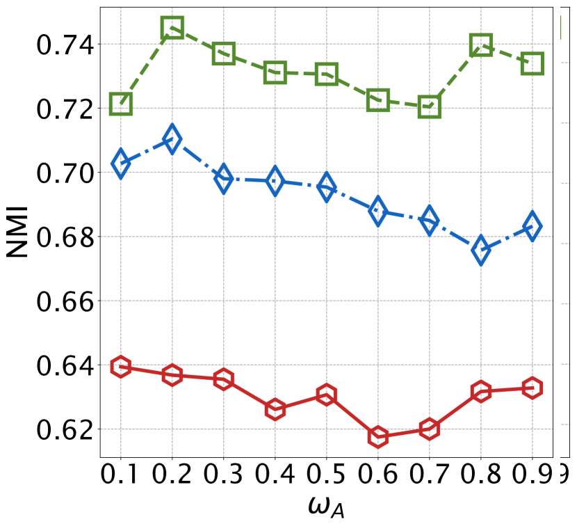
(c) Wiki-A Dataset

(d) Wiki-B Dataset

Figure 7: The effect of pre-training parameters in MLAS. The pre-training parameter $\omega_{A}$ decides the relative importance of attributes in the model. We observe that MLAS-A is capable of achieving the best performance on AMS-A and AMS-B datasets while MLAS-S has the best performance on Wiki-A and Wiki-B datasets.

IV-D2 Performance in Clustering Tasks.

The primary parameter in HDBSCAN is the minimum cluster size [23], denoting the smallest set of instances to be considered as a group. Intuitively, while the minimum cluster size increases, each cluster may include instances that do not belong to it and the performance decreases. Figure 5 presents the results with the output dimension is 10 and $\omega_{A}=0.5$.

Compared to the best baseline method ASF, MLAS-A achieves up to 18.3% and 25.4% increase of performance on AMS-A and AMS-B datasets, respectively. On Wiki-A and Wiki-B datasets, MLAS-S is capable of achieving up to 26.3% and 24.8% performance improvement compared to ASF, respectively. We further confirm that MLAS network is capable of exploiting the attribute-sequence dependencies to improve the performance of the clustering algorithm with various parameter settings.

IV-D3 Output Dimensions.

We evaluate MLAS under a wide range of output dimension choices. The number of output dimensions relates to a variety of impacts, such as the usability of feature representations in downstream data mining tasks. In this set of experiments, we fix the minimum cluster size at 50, $\omega_{A}=0.5$ and vary output dimensions from 10 to 100. From Figure 6 we conclude that our proposed approaches outperform the baseline methods with various output dimensions.

In particular, compared to the baseline method with the best performance, namely ASF, MLAS-A achieves 20.7% improvement on average on AMS-A dataset and 19.4% improvement on average on the AMS-B dataset. When evaluated using Wiki-A and Wiki-B datasets, MLAS-S outperforms ASF by 20.8% and 10.6% on average.

(a) ATT
without Feedback

(b) SEQ
without Feedback

(c) ASF
without Feedback

(d) MLAS-B
without Feedback

(e) MLAS-A
without Feedback

(f) MLAS-S
without Feedback

(g) ATT
with Feedback

(h) SEQ
with Feedback

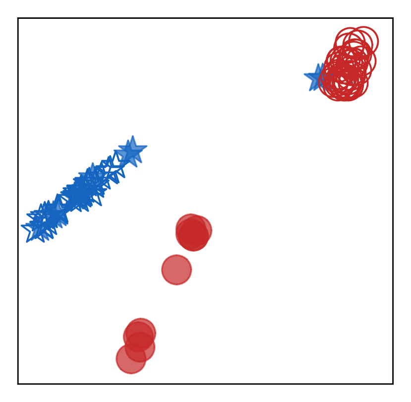
(i) ASF
with Feedback

(j) MLAS-B
with Feedback

(k) MLAS-A
with Feedback

(l) MLAS-S
with Feedback

Figure 8: Plots of the feature representations. The MLAS is capable of exploiting the feedback and separating the instances from two different groups while keeping the instances from the same group together.

IV-D4 Pre-training Parameters

We evaluate MLAS under different pre-training parameters in this set of experiments. ATT and SEQ are not included in this set of experiments since they only utilize one data type. Output dimension is set to 5. Minimum cluster size is set at 50. Figure 7 presents the results under different pre-training parameters. This confirms that our proposed MLAS method is not sensitive to different pre-training parameters.

We notice the performance differences among the three MLAS architectures in the above experiments, where MLAS-A has the best performance on AMS-A and AMS-B datasets, and MLAS-S has the best performance on Wiki-A and Wiki-B datasets. We conclude this difference may relate to the datasets.

IV-E Case Studies

In Figure 8, we apply t-SNE [25] to the feature representations generated by all compared methods. The set of feature representations without feedback is generated after the pre-training phase and before the distance metric learning process.

Our goal is to demonstrate the differences in the feature space of each method. We randomly select data points from both training and testing sets with a ground truth of two groups. We have the following findings:

1. The methods using either attribute data (ATT) or sequence data (SEQ) only cannot use the attributed sequence feedback.

2. The method using both attributes and sequences separately (ASF) is capable of better separating the two groups than the methods using single data type (ATT and SEQ).

3. Our methods using attributed sequence feedback as a unity to train unified models (MLAS-B/A/S) are capable of separating the two groups the furthest, and thus achieve the best results.

These observations confirm that all three designs of MLAS can effectively learn the distance metric and result in better separation of two groups of data points.

V Related Work

V-A Distance Metric Learning

Distance metric learning, with the goal of learning a distance metric from pairs of similar and dissimilar examples, has been extensively studied  [7, 3, 8, 2, 9, 4, 5, 6, 26]. The common objective of these tasks is to learn a distance metric so that the distance between similar pairs is reduced while the distance between dissimilar pairs is enlarged. Distance metric learning has been used to improve the performance of mining tasks, such as clustering [7, 3, 8]. Many application domain require distance metric learning, including patient similarity in health informatics [2], face verification in computer vision [9, 4, 5], image recognition [27] and sentence semantic similarity analysis [6, 26]. Recent works on distance metric learning using deep learning techniques have been using using siamese neural networks with two identical base networks in various supervised tasks [27, 6, 5, 28]. However, each of these works [27, 6, 5] focuses on a domain-specific problem with a homogeneous data type. Thus, the dependency challenge remain unexplored in these works.

V-B Deep Learning

Deep learning has received significant interests in recent years. Deep learning models are capable of feature learning with varying granularities. Various deep learning models and optimization techniques have been proposed in a wide range of applications from image recognition [29, 30] to sequence learning [31, 32, 33, 26, 34]. Many applications involve the learning of a single data type [31, 32, 33, 26], while some applications involve more than one data type [29, 30]. Several works [5, 6, 26] focus on deep metric learning using deep learning techniques. However, none of these works address the deep metric learning of more than one type of data nor the dependencies between different types of data.

VI Conclusion and Future Work

In this work, we focus on the novel problem of distance metric learning on attributed sequences. We first identify and formally define this prevalent data type of attributed sequences and the problem. We then propose one MLAS with three solution variations to this problem using neural network models. The proposed MLAS network effectively learns the nonlinear distance metric from both attribute and sequence data, as well as the attribute-sequence dependencies. In our experiments on real-world datasets, we demonstrate the effectiveness of our MLAS network over other state-of-the-art methods in both performance evaluations and case studies.

The prevalence of attributed sequence data and the broad spectrum of real-world applications using attributed sequences motivate us to keep exploring this new direction of research. Given the performance boost using attributed sequences and different variations of neural network models, future research could focus on exploring different design choices of the MetricNet. It would also be interesting to explore the design of alternative neural network models as the components within MLAS, such as AttNet and SeqNet. Another research topic would be the theoretical analysis of the performance differences among the three MLAS network architectures.

References

- [1] F. Wang and J. Sun, “Survey on distance metric learning and dimensionality reduction in data mining,” Data Mining and Knowledge Discovery, vol. 29, no. 2, pp. 534–564, 2015.
- [2] F. Wang, J. Sun, and S. Ebadollahi, “Integrating distance metrics learned from multiple experts and its application in patient similarity assessment,” in International Conference on Data Mining (SDM). SIAM, 2011, pp. 59–70.
- [3] D.-Y. Yeung and H. Chang, “A kernel approach for semisupervised metric learning,” IEEE Transactions on Neural Networks, vol. 18, no. 1, pp. 141–149, 2007.
- [4] M. Koestinger, M. Hirzer, P. Wohlhart, P. M. Roth, and H. Bischof, “Large scale metric learning from equivalence constraints,” in IEEE Conference on Computer Vision and Pattern Recognition (CVPR), 2012, pp. 2288–2295.
- [5] J. Hu, J. Lu, and Y.-P. Tan, “Discriminative deep metric learning for face verification in the wild,” in IEEE Conference on Computer Vision and Pattern Recognition (CVPR), 2014, pp. 1875–1882.
- [6] J. Mueller and A. Thyagarajan, “Siamese recurrent architectures for learning sentence similarity.” in AAAI Conference on Artificial Intelligence, 2016, pp. 2786–2792.
- [7] E. P. Xing, M. I. Jordan, S. J. Russell, and A. Y. Ng, “Distance metric learning with application to clustering with side-information,” in Neural Information Processing Systems (NIPS), 2003, pp. 521–528.
- [8] J. V. Davis, B. Kulis, P. Jain, S. Sra, and I. S. Dhillon, “Information-theoretic metric learning,” in International Conference on Machine Learning (ICML), 2007, pp. 209–216.
- [9] A. Mignon and F. Jurie, “Pcca: A new approach for distance learning from sparse pairwise constraints,” in IEEE Conference on Computer Vision and Pattern Recognition (CVPR), 2012, pp. 2666–2672.
- [10] D. Kedem, S. Tyree, F. Sha, G. R. Lanckriet, and K. Q. Weinberger, “Non-linear metric learning,” in Neural Information Processing Systems (NIPS), 2012, pp. 2573–2581.
- [11] J. Wang, A. Kalousis, and A. Woznica, “Parametric local metric learning for nearest neighbor classification,” in Neural Information Processing Systems (NIPS), 2012, pp. 1601–1609.
- [12] R. Chatpatanasiri, T. Korsrilabutr, P. Tangchanachaianan, and B. Kijsirikul, “A new kernelization framework for mahalanobis distance learning algorithms,” Neurocomputing, vol. 73, no. 10, pp. 1570–1579, 2010.
- [13] A. Graves, “Generating sequences with recurrent neural networks,” arXiv preprint arXiv:1308.0850, 2013.
- [14] T. Pham et al., “Column networks for collective classification,” in AAAI, 2017.
- [15] S. Hochreiter and J. Schmidhuber, “Long short-term memory,” Neural computation, vol. 9, no. 8, pp. 1735–1780, 1997.
- [16] R. Hadsell, S. Chopra, and Y. LeCun, “Dimensionality reduction by learning an invariant mapping,” in IEEE Conference on Computer Vision and Pattern Recognition (CVPR), 2006, pp. 1735–1742.
- [17] “Amadeus IT Group,” http://www.amadeus.com, 2017, accessed: 2017-09-23.
- [18] R. West, J. Pineau, and D. Precup, “Wikispeedia: An online game for inferring semantic distances between concepts,” in International Joint Conference on Artificial Intelligence (IJCAI), 2009.
- [19] D. Erhan, P.-A. Manzagol, Y. Bengio, S. Bengio, and P. Vincent, “The difficulty of training deep architectures and the effect of unsupervised pre-training,” in International Conference on Artificial Intelligence and Statistics (AISTATS), 2009, pp. 153–160.
- [20] X. Glorot and Y. Bengio, “Understanding the difficulty of training deep feedforward neural networks,” in International Conference on Artificial Intelligence and Statistics (AISTATS), 2010, pp. 249–256.
- [21] A. M. Saxe, J. L. McClelland, and S. Ganguli, “Exact solutions to the nonlinear dynamics of learning in deep linear neural networks,” arXiv preprint arXiv:1312.6120, 2013.
- [22] V. Nair and G. E. Hinton, “Rectified linear units improve restricted boltzmann machines,” in International Conference on Machine Learning (ICML), 2010, pp. 807–814.
- [23] R. Campello, D. Moulavi, A. Zimek, and J. Sander, “Hierarchical density estimates for data clustering, visualization, and outlier detection,” in Transactions on Knowledge Discovery from Data (TKDD). ACM, 2015.
- [24] A. F. McDaid, D. Greene, and N. Hurley, “Normalized mutual information to evaluate overlapping community finding algorithms,” arXiv preprint arXiv:1110.2515, 2011.
- [25] L. v. d. Maaten and G. Hinton, “Visualizing data using t-sne,” Journal of Machine Learning Research (JMLR), vol. 9, no. Nov, pp. 2579–2605, 2008.
- [26] P. Neculoiu, M. Versteegh, M. Rotaru, and T. B. Amsterdam, “Learning text similarity with siamese recurrent networks,” Annual Meeting of the Association for Computational Linguistics (ACL), p. 148, 2016.
- [27] G. Koch et al., “Siamese neural networks for one-shot image recognition,” in ICML deep learning workshop, vol. 2, 2015.
- [28] Z. Zhuang, X. Kong, E. Rundensteiner, A. Arora, and J. Zouaoui, “One-shot learning on attributed sequences,” in 2018 IEEE International Conference on Big Data (Big Data). IEEE, 2018, pp. 921–930.
- [29] A. Karpathy and L. Fei-Fei, “Deep visual-semantic alignments for generating image descriptions,” in IEEE Conference on Computer Vision and Pattern Recognition (CVPR), 2015, pp. 3128–3137.
- [30] K. Xu, J. Ba, R. Kiros, K. Cho, A. Courville, R. Salakhudinov, R. Zemel, and Y. Bengio, “Show, attend and tell: Neural image caption generation with visual attention,” in International Conference on Machine Learning (ICML), 2015, pp. 2048–2057.
- [31] K. Cho, B. van Merrienboer, C. Gulcehre, D. Bahdanau, F. Bougares, H. Schwenk, and Y. Bengio, “Learning phrase representations using rnn encoder–decoder for statistical machine translation,” in Empirical Methods on Natural Language Processing (EMNLP), 2014, pp. 1724–1734.
- [32] I. Sutskever, O. Vinyals, and Q. V. Le, “Sequence to sequence learning with neural networks,” in Neural Information Processing Systems (NIPS), 2014, pp. 3104–3112.
- [33] Y. Xu, J. H. Lau, T. Baldwin, and T. Cohn, “Decoupling encoder and decoder networks for abstractive document summarization,” MultiLing 2017, p. 7, 2017.
- [34] Z. Zhuang, X. Kong, and E. Rundensteiner, “AMAS: Attention model for attributed sequence classification,” in International Conference on Data Mining (SDM). SIAM, 2019.