Dynamical Dark Energy Properties Hidden in the Dark Matter Halos and Voids

Abstract

In this paper, we analysed the halos and voids properties of a GR-based N-body simulation carried out at redshifts $z=0.0$ and $z=0.8$ as differences between dynamical dark energy models (namely PL and CPL) with respect to $\Lambda CDM$. Analysing the halos demonstrates that both models, PL and CPL, behave like $\Lambda CDM$, despite the velocity dispersion of halos was more sensitive to the dynamical dark energy model. In addition, a void finder was developed to extract the properties of voids from simulated data. Further statistical model on voids confirms that the PL model produces larger voids. In summary, our novel simulation demonstrates void properties are better than halo properties in discriminating between dark energy models. Hence, the results suggest to make more use of the properties of voids in future studies of discriminating dynamical dark energy models.

1 Introduction

The cosmological constant was historically introduced to allow for obtaining a static solution of the Fridman equations, but it received more attention after the discovery of the acceleration of the expansion(Riess et al., 1998; Perlmutter et al., 1999). Various scientific projects such as the DESI Flaugher & Bebek (2014), the WiggleZ Parkinson et al. (2012),the Destiny Benford & Lauer (2006) and the Planck Ade et al. (2016) were carried out not only to assess the source of expansion but also to achieve desired observational accuracy (Cheng & Huang, 2015). However, the $\Lambda CDM$ model is a simple and well defined model which is consistent with the majority of current cosmological observations. However, it suffers from some problems such as the sharp transition from the cold dark matter era to $\Lambda$ the dominant epoch and the fine-tuning (Martin, 2012; Kunz, 2012). Besides, there are some reports on flowing tension: the excessive congestion of the matter and the missing satellites puzzle Moore et al. (1999); Klypin et al. (1999), the cusp-core problem (Navarro et al., 1996) and in reliable observational projects run by the $Planck$ collaboration, the observed clusters are fewer than what was expected (Ade et al., 2016). There is a tension between the value of the Hubble constant from local distance indicators as the late time data and the angular scale of fluctuations in the Cosmic Microwave Background in early time data Freedman (2017); Mörtsell & Dhawan (2018); Ebrahimi et al. (2020). Due to the mentioned problems, $\Lambda$ can be considered as a variable quantity rather than a constant value. Hence, reconstruction of the equation of state based on observations (Huterer & Turner, 1999) and model parameters estimation (Nair et al., 2014) are performed to alleviate the problems.
The important effects of dark energy on structures are in the red-shift evolution of the linear growth factor and the evolution of perturbations which are sensitive to the dark energy equation of state. The statistical analysis of dark energy properties mainly focused on highly dense regions such as the galaxy number density, two-point correlation function, and gas galaxy clusters (McClintock et al., 2018; Benson et al., 2018). The cosmological peculiar velocity of dark matter halo carries significant information on the theory of gravity and dark energy in large scales Nusser et al. (2013). Furthermore, the evolution of dark energy filed value produces a term which decreases or increases the peculiar velocity (Farrar & Peebles, 2004). The suppression or enhancement peculiar velocity depends on whether $w>-1$ or $w<-1$ compared with $\Lambda CDM$ Xu et al. (2013). Moreover, extra sensitivity of voids to the dark energy equation of state has been determined (Lavaux & Wandelt, 2010, 2012). Recent research points out that cosmic voids not only show a key component of the mass distribution but also are one of the cleanest demonstrations of the dark energy’s nature (Bos et al., 2012). Voids provide an opportunity to investigate dark energy properties without any new survey. In addition, it has been demonstrated voids abundance noticeably do tighter constraints on free parameters of the dark energy equation of state Pisani et al. (2015). Using voids as a cosmological probe can lead to some complications as the void definition and the void finding since voids are not well-defined and unbounded systems. The void has been classified into three categories: firstly, it determines the empty regions of the universe, secondly, one tries to find voids as a geometrical structure in dark matter, and thirdly, it checks unstable points in the distribution of galaxies (Lavaux & Wandelt, 2010; Colberg et al., 2008).
Releasing of the large public catalogue (Pan et al., 2012; Sutter et al., 2012a, b) from the Solan Digital Survey (SDSS) provides a comparison of the simulation with data and highlights the importance of N-body simulations for studying void properties.
Moreover, several attempts has been done to extract voids on cosmological data. Two methods have been developed to extract voids in Dark Energy Survey (DES). Further, the relation of mass and galaxies profile of cosmic voids base on N-body simulation and 3D distribution of galaxies has been studied Fang et al. (2019). In addition, an algorithm of void finder developed and applied to photometric DES-SV data in the redshift range $0.2<z<0.8$ Sánchez et al. (2016). A void size function model has been developed on simulation of dark matter halo which calibrated on the halo catalogue and the method is a critical step in applying to real data Contarini et al. (2019).
The cosmic voids give us an opportunity to study massive neutrino. Neutrino free steaming in the voids is more easily rather than the dark matters and the baryons. It has been shown that the characteristics of the voids are affected by neutrino through DEMNUni simulations (Schuster et al., 2019). Besides, the theoretical description of the void size function instead of direct simulation of halo catalogue in DEMNUni simulations have been tested Verza et al. (2019).
Several existing void finder algorithms have been tested to check the potential power of discrimination between General Relativity and modified gravity. They found the voids profile of f(R) theory is more underdense rather than General Relativity. They further investigated the potential of each void finder to test f(R) in the near future survey as Euclid and LSST Cautun et al. (2018).

There are a vast number of void finder algorithms based on finding the minimum underdensity working on unsmooth particles Neyrinck (2008); Sutter et al. (2015) or a well-known technique for the segmentation of images Platen et al. (2007). (Colberg et al., 2008) presents the systematic comparison of 13 voids finders using particles and halos and found that various methods are in agreement.

At present, N-body simulations for studying the structure formation still employ the Newtonian approximation (Springel et al., 2001; Schmidt, 2009; Li et al., 2012) which impose restrictions on the nature of dark energy and dark matter. Newtonian N-body simulations are non-relativistic Springel (2005) and could not compute the essential relativistic nature of scalar fields Noller et al. (2014). To predict and compare the upcoming observations from galactic and cluster scale in non-linear regimes, N-body simulations are required to solve scalar field equations Llinares et al. (2014). Hence, quasi statistic approximation was added to Newtonian simulations Llinares et al. (2014); Puchwein et al. (2013), despite it leads to high computational time cost Brax et al. (2013); Noller et al. (2014). Furthermore, Newtonian simulations work on the background evolution of Universe Pollina et al. (2016) and they fail to describe the dark energy clustering in perturbation level which is an important aim of upcoming surveys such as Euclid Laureijs et al. (2011). Gevolution is the first N-body code that considers all the six degrees of freedom in the metric and solves the geodesic equation. It takes into account the relativistic potential which is sensitive to the dark energy equation of state and it is more appropriate for the dark energy scenario (Adamek et al., 2016a). Recently, a relativistic N-body code for the clustering of dark energy has been developed Hassani et al. (2019). It is based on the Gevolution and focuses on k-essence dark energy.

In this paper, we focus on N-body simulation of the dynamical dark energy models based on General Relativity with Gevolution and use the void finder which works with an unsmooth particle distribution without any prior spherical shape.We also utilize the halo finder analysis to extract the statistical properties of the dark matter halo for the models. Then, we employ the void finder based on the Alikio and Mahonen method to explore voids’ size and density distributions for the dynamical dark energy and $\Lambda CDM$ models. The chosen models in this study are Chavelier-Polarski-Linder (CPL) and Power Law (PL). Measurement of free parameters of the model from combination of SNIa+BAO+HST+PlanckTT+LSS observation data sets are obtained Ebrahimi et al. (2018). The model has quite a different equation of state from $\Lambda$CDM. The CPL equation of state remains always below of $w=-1$ and the PL equation of state crosses $w=-1$. Due to the crossing behavior of PL, the model has a positive equation of state at early times and enhances the matter component of the early Universe, leading it to naturally behaves similarly to coupled dark energy- dark matter models without introducing any extra coupling parameter.In section 2, we present the dark energy models. We intend to simulate the reported observational constraints on their free parameters. In section 3, we investigate the properties of N-body simulation. Then, the results of the halo finder and void finder are presented in section 4. The discussion are given in section 5. Finally, we conclude the main findings in section 6.

2 THEORY

Dark energy properties are often characterized by the equation of state ($w(z)$), which introducing different parameterization of equation of state. It allows us to illustrate the Universe evolution. Also, the sound speed ($c_{s}^{2}$) causes clustering of dark energy, and anisotropic pressure ($\sigma$). Anisotropic pressure appear when the first order of the perturbation is considered. Dynamical dark energy models can be distinguished from $\Lambda$CDM through a variable equation of state and non-zero sound speed. The anisotropic pressure is zero in the dark energy models we simulated. The models that are considered in this study are as following:

2.1 CPL model

Reconstruction of equation of state is a viewpoint which extract the property of dark energy as a component of the Universe. Equation of state can parameterized by using free parameters which its number depends on theoretical or phenomenological approach. Fist equation of state was proposed by Linder (2003b) base on linear series of redshift and suffer divergence at high redshift. Then, Chavelier-Polarski-Linder model (CPL) has been proposed to explore the dynamical behavior of dark energy with the following equation of state (Chevallier & Polarski, 2001; Linder, 2003a):

$$w_{\rm CPL}(z)=w_{0}+w_{1}\dfrac{z}{1+z}.$$ (1)

where $w_{0}$ and $w_{1}$ are the free parameters of the model. It covers many scalar field EoS with high accuracy. It has manageable two dimensional phase space, bounded at high redshift and widely used Vazquez et al. (2012); Sahni et al. (2008); Bengaly et al. (2020a, b). However, it suffers from a divergence at $z=-1$. The CPL model is in subclass of quintessence and its Lagrangian ca be found Ma & Zhang (2011).

2.2 PL model

Power law (PL) model is parametrized to solve the fine tuning problem. The PL model does not suffer the fine tuning problem because the ratio of the dark energy density to the matter density is not sensitive to the free parameters of the model and asymptotically goes to zero at the early epochs. Also, the model solves the age of old star problem known as cosmic age crisis. The PL model equation of state has a crossing $w=-1$ behaviour which leads the dark matter effect at early universe and behaves same as coupled dark matter-dark energy models without any coupling parameter. The equation of state of the model is given by (Rahvar & Movahed, 2007):

$$w_{\rm PL}(z)=\frac{w_{0}}{(1+z)^{\alpha}}[1-\alpha\ln\left(1+z\right)].$$ (2)

where $w_{0}$ and $\alpha$ are the model’s free parameters. The Lagrangian of the model can be found in (Rahvar & Movahed, 2007).
The observational constraints on the free parameters of the models that are the subject of our interest in this work are given in Table 1.

Table 1: Observational constraints on the free parameters of the PL and CPL models using SNIa+BAO+HST+PlanckTT+LSS data employing the Markov Chain Monte Carlo method.

Parameter	PL	CPL
$w_{0}$	$-1.3799^{+0.0036}_{-0.0028}$	$-1.08045^{+0.00041}_{-0.00062}$
$w_{1}$	-	$-0.12190^{+0.00050}_{-0.00030}$
$\alpha$	$0.1013\pm 0.0031$	-
$\Omega_{DM}$	$0.1195\pm 0.0013$	$0.1193^{+0.0014}_{-0.0017}$
$\Omega_{DE}$	$0.6862\pm 0.0078$	$0.688^{+0.010}_{-0.0079}$
$H_{0}$	$67.36\pm 0.56$	$67.48^{+0.71}_{-0.57}$

Figure 1: The top panel shows the map density of dark matter through N-body simulation of $\Lambda CDM$ by Gevolution at $z=0$. the side size is 256 Mpc/h. The bottom panel is the voids visualization of $\Lambda CDM$ based on the simulation at $z=0.0$

h

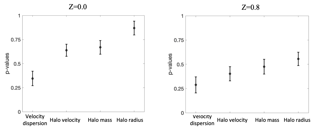
Figure 2: Plot shows the p-values of the Kruskal-Wallis test that compared the median of three models for velocity dispersion, halos velocity, halos mass and halo radius through 10 simulation boxes in two redshifts $z=0.00$ (left panel) and $z=0.8$ (right panel), both at 1 $\sigma$ confidence level.

3 SIMULATIONS

Upcoming surveys will observe the Universe with higher accuracy and more precision in the non-linear regime Adam et al. (2016); Carilli & Rawlings (2004), namely, the Euclid will accomplish a spectroscopic redshift survey of 50 million galaxies over a volume 500 times larger than the SDSS. The spectroscopic survey will be received with a redshift accuracy $\sigma_{z}/(1+z)\leqslant 0.001$. Also, observing galaxies are over $75\%$ of the lifetime of the Universe. Furthermore, the precision of photometric redshifts for these galaxies reaches $\sigma_{z}/(1+z)<0.05$ Laureijs et al. (2011). Despite Non-linear scales are challenging, they are worth working on through N-body simulations. The various simulation strategies address different problems in this regime depending on the goal of the study. In general, N-body simulations are based on Newtonian gravity or post-Newtonian gravity (Springel et al., 2001; Schmidt, 2009; Li et al., 2012). They work on the background evolution of the Universe and fail to describe dark energy as a scalar field and its perturbation. In 2016, (Adamek et al., 2016b) introduced Gevolution which is a N-body simulation code based on General Relativity framework. The code is based on a weak field expansion of General Relativity and calculates all six metric degrees of freedom in Poisson gauge. It addresses a more general solution among the rest of the structure formation simulations. Gevolution is an appropriate choice for studying models with dynamical dark energy or with modified gravity and it is claimed to be computationally fast enough. There are several comparisons about the speed in Adamek et al. (2016b).

We modified Gevolution at the background evolution according t0 the mentioned dynamical dark energy models. The side of simulation boxes is 256 Mpc/h and contains $512^{3}$ particles using 1 Mpc/h resolution for fields taking 265 CPU hours of execution time. To assess the homogeneity of the simulation, the simulation was run 10 times with different number of seeds. Then, we applied halo finder algorithms (is explained below) to particles of 10 boxes and analysed the p-value of the dark matter halos properties. Finally, we performed the void finder analyse and compared the properties of halos and voids of the dark energy models with respect to $\Lambda CDM$.

4 RESULTS

4.1 Rockstar Halo finder Analysis

Since the dark matter halos carry a significant information regarding cosmology, to compare dark matter statistics with void results we analysed dark matter halo properties distribution employing the Rockstar (Robust over density Calculation using K-Space topologically adaptive refinement) halo finder for the models Behroozi et al. (2012). The Rockstar is an algorithm to identify the dark matter halos and their substructures. It is based on the adaptive hierarchical refinement of friends-of-friends groups in seven dimensions (phase-space+time). This algorithm is very good at the substructure recovery. The Rockstar separates particles to friends-of-friends groups at the very early step then performs subgroup detection in natural phase space. This step repeats until it finds all substructures. The Rockstar is efficiently parallel and can be run on high resolution simulations and can be used to analyse the performance of halos .

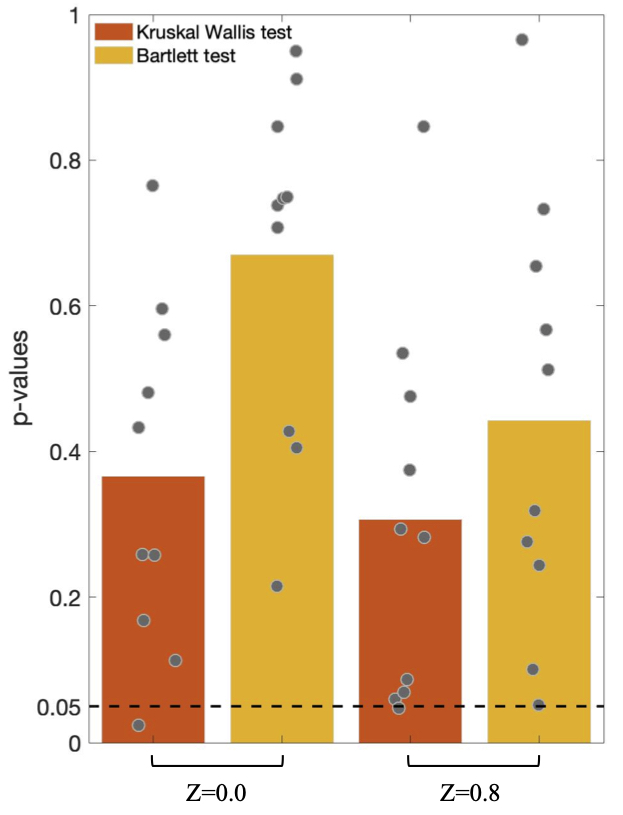
Figure 3: The bar-graph shows the homogeneity evaluation of the velocity dispersion. This exhibits p-values of two statistical tests, Kruskal-Wallis test and Bartlett test, applied to the velocity dispersion of three models obtained via 10 simulations at two redshifts $z=0.0$ and $z=0.8$.

Figure 4: The top row shows the probability distribution functions (PDFs) of the velocity dispersion obtained from the simulation of three models, LCDM, CPL and PL in two redshifts $z=0$ (left panel) $z=0.8$ (right panel). The below plots exhibit the median and interquartile range of the models’ density of voids at two thresholds ( $z=0$ and $z=0.8$).

The Rockstar halo catalogue aims to provide a history for each halo and gives us more information such as position, halos mass, radius, velocity, and velocity dispersion. We found among all properties, velocity dispersion is sensitive to the dark energy models. The fig. 3 shows the mean p-value of Kruskal-Wallis test that compared the velocity dispersion, halos velocity, halos mass, and halo radius obtained from three models, $\Lambda$CDM, CPL and PL via 10 simulation boxes at two redshifts with 1 $\sigma$ confidence level. This indicates that among the mentioned properties, the velocity dispersion with smaller p-values is more sensitive in discriminating the dark energy models, despite the fact that the properties of all models were significantly equal.
Figure 3 compares the p-values of two statistical tests, Kruskal-Wallis and Bartlett, to evaluate the equality of the medians and variances of velocity dispersion between three proposed models at each simulation at two redshifts. No significant difference were observed between calculated p-values (Wilcoxon signed-rank test against $p=0.05$, $p>0.34$). These test confirm that the simulations are homogeneous and we are allowed to select one of the simulations for further analysis of the void finder.
Velocity dispersion is defined as the sum in quadrature of the component-wise velocity standard deviations:

$$v_{d}=\sqrt{\sigma_{vx}^{2}+\sigma_{vy}^{2}+\sigma_{vx}^{2}}$$ (3)

The probability distribution functions (PDFs) of velocity dispersion for two redshift are shown in the top panels of figure 4. The below plots exhibit the median and interquartile range of the models’ velocity dispersion at two redshifts with 1 $\sigma$ confidence level. Despite the velocity dispersion of three models at two reshshift is not Gaussian, they are equally distributed in the same range of the velocity (Kolmogorov–Smirnov test, $p>0.05$). Moreover, we did not find any statistical difference between the velocity dispersion of two models CPL and PL and the velocities velocity dispersion of the $\Lambda$ CDM when a non-paramteric test, wilcoxon rank sum test, applied to the velocity dispersions to compare their medians (Figure 4, $p>0.05$). The statistical values of the wilcoxon rank sum test of the velocity dispersion (SWV) of dark matter halos for the given dark energy models with respect to $\Lambda$ CDM. is reported in Table 2.

4.2 Void Finder Algorithm

In order to evaluate the potential impact of the models introduced in section 2 on cosmological structures, we compared the properties of voids extracted in the models. To do that, we employed the algorithm developed in Tavasoli et al. (2013), which is an updated 3D version of the earlier 2D void finding algorithm Alikio and Mahonen (AM) Aikio J. (1998). We emphasize that we considered the AM statistics just as a tools for the relative (not absolute) measurement of some properties of voids (e.g. effective radius and density contrast) in all simulated catalogues. Prior to applying the AM algorithm to the three models, the simulated box sample was girded up to cells of 1 Mpc/h as. The algorithm works through the first distinguishing between wall and field halos by considering distances to the third nearest neighbour Hoyle & Vogeley (2002). Voids were then identified by the following algorithm. Initially, a Cartesian grid was created and distances from grid cells to wall halos were identified. Each grid cell was then assigned to a sub void by applying the climbing algorithm Schmidt et al. (2001) to reach the grid cell with the locally-largest distance to the wall. If the distance between two sub voids was smaller than their distances to walls, they were combined into a single void. Finally, all field halos residing within voids were labeled as void halos. This generated void catalogue, includes variety of voids in size $R_{v}$, and number density contrast $\delta_{v}$. The number density contrast of a void is defined by $\delta_{v}=(\rho_{v}-\rho_{m})/\rho_{m}$ where $\rho_{v}$ is given by the ratio of the total number of halos inside a given void by the volume of that void and $\rho_{m}$ is mean number density of the samples. For each void, we defined its effective radius $R_{v}$ as the radius of a sphere whose its volume was equal to the void. In order to avoid counting spurious voids in our catalogue, the size of voids was considered to be be larger than $R_{v}>7Mpc/h$.
The probability distribution functions (PDFs) of effective radius and density contrast are shown in top panel of figures 6 and 6 for two redshifts bin while the below plots exhibit the median and interquartile range of the models effective radius and density contrast with 1 $\sigma$ confidence level. Both the effective radius and the density contrast of three models were distributed equally in the same range (Kolmogorov–Smirnov test, $p>0.05$). Although the shape of the distributions are statistically same, the effective radius of the PL models are larger than the radius in $\Lambda$ CDM (Figure 6, Wilcoxon rank sum test, $p=0.02$). However, no difference was observed in other properties (Table 2). Besides, the statistical values of the Wilcoxon rank sum test of effective radius (SWR) and density contrast (SWD) of voids of dynamical dark energy model against $\Lambda$ CDM is reported in the table 2.

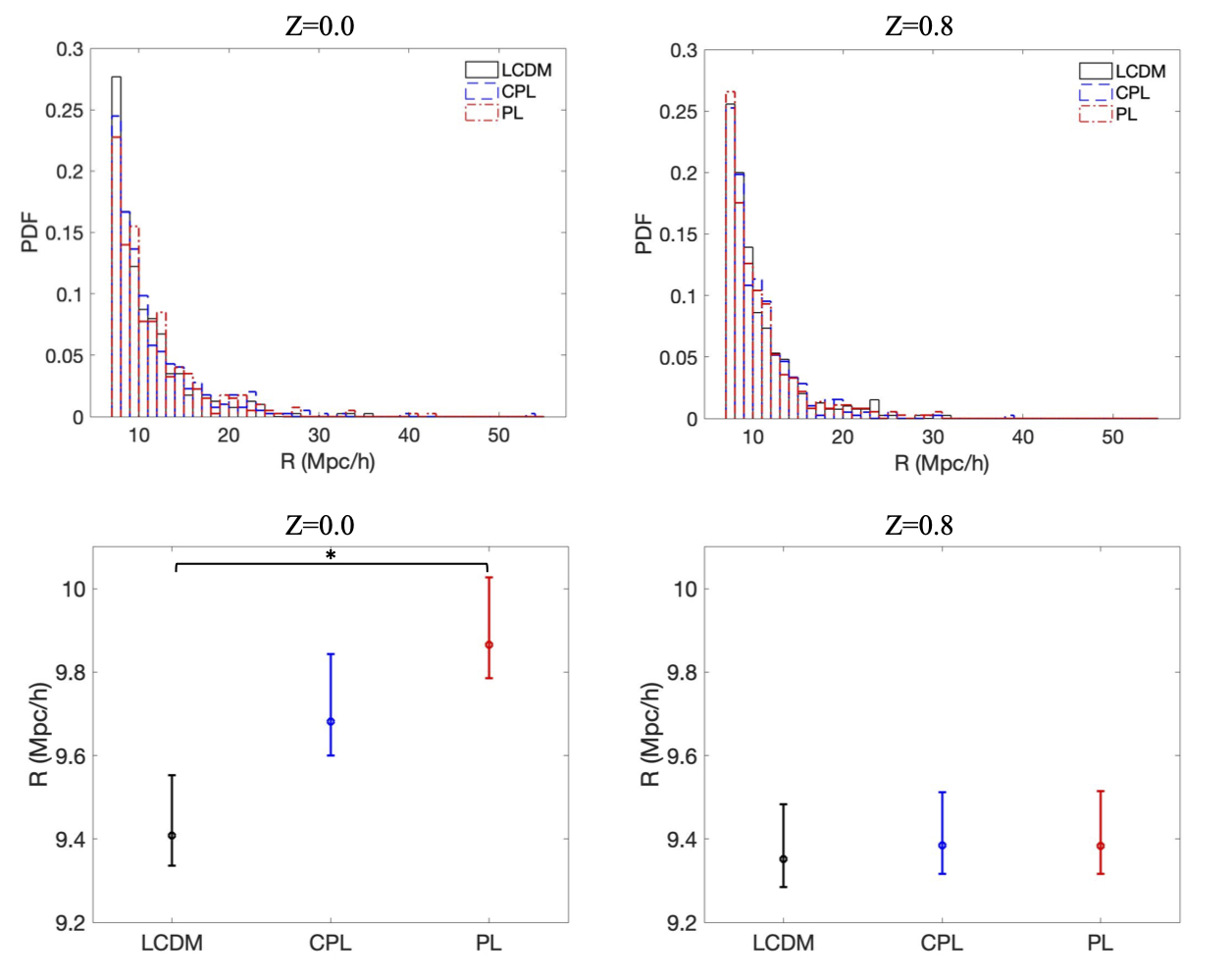
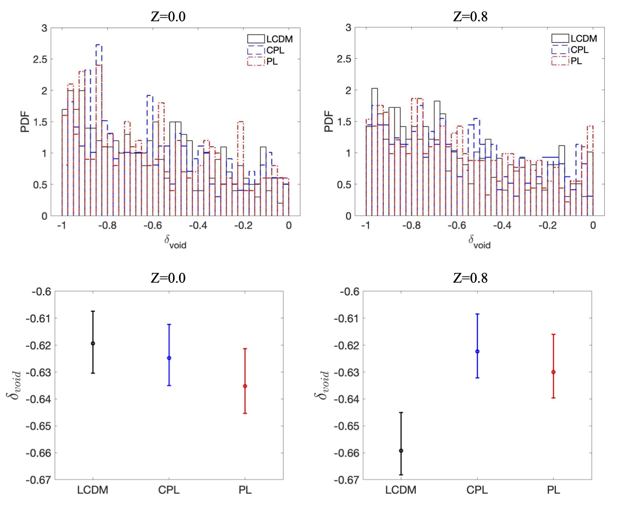
Figure 5: The top row shows the probability distribution functions (PDFs) of the effective radius of three models, LCDM, CPL and PL at two redshifts $z=0$ (left panel) $z=0.8$ (right panel). The below plots exhibit the median and interquartile range of the models’ effective radius at two thresholds (left: $z=0$; right: $z=0.8$), all with 1 $\sigma$ confidence level. This indicates that only the PL model produced larger void compared with other models ($p=0.02$).

Figure 6: The top row shows the probability distribution functions (PDFs) of the density of voids of three models, LCDM, CPL and PL at two redshifts $z=0$ (left panel) $z=0.8$ (right panel). The below plots exhibit the median and interquartile range of the models’ density of voids at two thresholds (left: $z=0$; right: $z=0.8$) with 1 $\sigma$ confidence level.

Table 2: The table shows the statistical value of the wilcoxon rank sum test of effective radius (SWR), density of voids (SWD) and the velocity dispersion (SWV) of dark matter halos for the given dark energy models, CPL and PL against $\Lambda CDM$.

Model	Voids				Halos
	SWR		SWD		SWV
	z=0.0	z=0.8	z=0.0	z=0.8	z=0.0	z=0.8
CPL	0.34	0.92	0.57	0.22	0.27	0.63
PL	0.022	0.79	0.69	0.31	0.11	0.13

5 DISCUSSION

In this research, we analysed the statistical properties of the dark matter halos and voids as discriminators of two dynamical dark energy models, CPL and PL, against $\Lambda CDM$ model.To analyse the statistical features of the halos and voids, we performed a N-body simulation based on General Relativity Adamek et al. (2016b) considering three models,$\Lambda CDM$, CPL and PL Rahvar & Movahed (2007); Chevallier & Polarski (2001); Ebrahimi et al. (2018) for the background evolution of the cosmology. The Rockstar Halo finding algorithm was used to extract the halos of the dark matter for these models. Then, properties of the halos, mass, radius, velocity, and velocity dispersion , were compared between three models. Although no difference between the properties of the halos obtained from the models was not observed (Fig 2), the p-values of the velocity depression was smaller compared to other properties. This suggested to consider the velocity depression as a sensitive indicator for further analysis in this study. However, two statistical methods were utilised to evaluate the homogeneity between all simulations (Fig 3). We found that there is no difference between all simulation. This allowed us to select one of these simulation for the next step analysing voids. Thought a searching algorithm developed for this study to find voids in the simulated data (see the Section 4), different set of voids were obtained for the models. To investigate the properties of the voids in the dark matter, the radius and density contrast of the voids are extracted. we found that although the both radius and density contrast of the models are equally distributed in the form (top Figs 6 and 6), the PL model garnered larger voids on average (bottom Fig 6). Since this study reports and compares the properties of the voids and halos generated from the General Relativity base simulation Adamek et al. (2016b) for the first time, we suggest properties of voids can provide the information same as the properties of the halos that is historically more common in the cosmology. Moreover, the developed void finder in this study along with the simulation can be considered as a good platform to explore and understand the dark energy properties in future.

Our simulation based on the General Relativity and the void finder algorithm are novel, there are still some limitations in the method of extracting voids’ properties. Our simulation was limited at only two redshift bin, $z=0.8$ and $z=0.0$. To track the evolution of halos and voids in the present of dynamical dark energy model, this will be useful to consider more redshifts bin. To speed up the simulation process, we considered 1 MPc/h for the resolution of both simulation and the void finder while this parameter can be varied in higher resolution, but with the expensive computational cost. Indeed, the higher resolutions using parallel processing will result in better discrimination of the voids’ radius (Fig 6). Moreover, the Gas was not included in the N-body simulation we used in this study. This causes a limitation to compare our result with the real observations data. In addition , we modified Genolution on background equations and did not employ perturbation of dark energy (i.e. in clustering dark energy). Adding the clustering of dark energy will be benefits to get more appropriate results.
Further study is required to complete our simulation with higher resolution N-body code and void finder and adding the clustering of dark energy models to investigate differences of the models respect to $\Lambda CDM$ which is one of the aim of Euclid project Laureijs et al. (2011).

6 CONCLUSIONS

We examined the dynamical dark energy effect on the voids and dark matter halo properties through N-body simulation in the General Relativity framework by the Gevolution. Our results demonstrate that the effective radius of voids is a better discriminator between the models investigated compared to the density contrast of voids at $z=0.0$. Our simulation shows PL model produces larger voids that is promising for further research. Indeed, adding the clustering of dark energy would be a good opportunity to extract differences for future data. We also found that the velocity dispersion of dark matter is the best halo properties among other properties, although, velocity dispersion could not be used as a discriminator of DE models from $\Lambda CDM$ at $z=0.8$ and $z=0.0$ (see Fig. 4) with a statistically significant confidence level.
We leave investigation of void properties by adding dark energy clustering through N-body simulation and using neural network to further studies.

References

- Adam et al. (2016) Adam R., et al., 2016, Astron. Astrophys., 594, A1
- Adamek et al. (2016a) Adamek J., Daverio D., Durrer R., Kunz M., 2016a, Nature Phys., 12, 346
- Adamek et al. (2016b) Adamek J., Daverio D., Durrer R., Kunz M., 2016b, JCAP, 1607, 053
- Ade et al. (2016) Ade P. A. R., et al., 2016, Astron. Astrophys., 594, A24
- Aikio J. (1998) Aikio J. M. P., 1998, ApJ, 497, 534
- Behroozi et al. (2012) Behroozi P. S., Wechsler R. H., Wu H.-Y., 2012, The Astrophysical Journal, 762, 109
- Benford & Lauer (2006) Benford D. J., Lauer T. R., 2006, in Space Telescopes and Instrumentation I: Optical, Infrared, and Millimeter. p. 626528
- Bengaly et al. (2020a) Bengaly C. A., Clarkson C., Kunz M., Maartens R., 2020a, arXiv preprint arXiv:2007.04879
- Bengaly et al. (2020b) Bengaly C. A., Clarkson C., Maartens R., 2020b, Journal of Cosmology and Astroparticle Physics, 2020, 053
- Benson et al. (2018) Benson A., Merson A., Wang Y., Faisst A., Masters D., Kiessling A., Rhodes J., 2018, in American Astronomical Society Meeting Abstracts.
- Bos et al. (2012) Bos E. G. P., van de Weygaert R., Dolag K., Pettorino V., 2012, Mon. Not. Roy. Astron. Soc., 426, 440
- Brax et al. (2013) Brax P., Davis A.-C., Li B., Winther H. A., Zhao G.-B., 2013, Journal of Cosmology and Astroparticle Physics, 2013, 029
- Carilli & Rawlings (2004) Carilli C. L., Rawlings S., 2004, New Astron. Rev., 48, 979
- Cautun et al. (2018) Cautun M., Paillas E., Cai Y.-C., Bose S., Armijo J., Li B., Padilla N., 2018, Monthly Notices of the Royal Astronomical Society, 476, 3195
- Cheng & Huang (2015) Cheng C., Huang Q.-G., 2015, Sci. China Phys. Mech. Astron., 58, 599801
- Chevallier & Polarski (2001) Chevallier M., Polarski D., 2001, Int. J. Mod. Phys., D10, 213
- Colberg et al. (2008) Colberg J. M., et al., 2008, Mon. Not. Roy. Astron. Soc., 387, 933
- Contarini et al. (2019) Contarini S., Ronconi T., Marulli F., Moscardini L., Veropalumbo A., Baldi M., 2019, Monthly Notices of the Royal Astronomical Society, 488, 3526
- Ebrahimi et al. (2018) Ebrahimi A. S., Monemzadeh M., Moshafi H., 2018, arXiv preprint arXiv:1802.05087
- Ebrahimi et al. (2020) Ebrahimi A., Monemzadeh M., Moshafi H., Movahed S. M. S., 2020, Mathematics Interdisciplinary Research, 5, 113
- Fang et al. (2019) Fang Y., et al., 2019, Monthly Notices of the Royal Astronomical Society, 490, 3573
- Farrar & Peebles (2004) Farrar G. R., Peebles P. J. E., 2004, Astrophys. J., 604, 1
- Flaugher & Bebek (2014) Flaugher B., Bebek C., 2014, in Ground-based and Airborne Instrumentation for Astronomy V. p. 91470S
- Freedman (2017) Freedman W. L., 2017, arXiv preprint arXiv:1706.02739
- Hassani et al. (2019) Hassani F., Adamek J., Kunz M., Vernizzi F., 2019, Journal of Cosmology and Astroparticle Physics, 2019, 011
- Hoyle & Vogeley (2002) Hoyle F., Vogeley M. S., 2002, The Astrophysical Journal, 566, 641
- Huterer & Turner (1999) Huterer D., Turner M. S., 1999, Phys. Rev., D60, 081301
- Klypin et al. (1999) Klypin A. A., Kravtsov A. V., Valenzuela O., Prada F., 1999, Astrophys. J., 522, 82
- Kunz (2012) Kunz M., 2012, Comptes Rendus Physique, 13, 539
- Laureijs et al. (2011) Laureijs R., et al., 2011, arXiv preprint arXiv:1110.3193
- Lavaux & Wandelt (2010) Lavaux G., Wandelt B. D., 2010, MNRAS, 403, 1392
- Lavaux & Wandelt (2012) Lavaux G., Wandelt B. D., 2012, The Astrophysical Journal, 754, 109
- Li et al. (2012) Li B., Zhao G.-B., Teyssier R., Koyama K., 2012, JCAP, 1201, 051
- Linder (2003a) Linder E. V., 2003a, Phys. Rev. Lett., 90, 091301
- Linder (2003b) Linder E. V., 2003b, Physical Review Letters, 90, 091301
- Llinares et al. (2014) Llinares C., Mota D. F., Winther H. A., 2014, Astronomy & Astrophysics, 562, A78
- Ma & Zhang (2011) Ma J.-Z., Zhang X., 2011, Physics Letters B, 699, 233
- Martin (2012) Martin J., 2012, Comptes Rendus Physique, 13, 566
- McClintock et al. (2018) McClintock T., et al., 2018, Submitted to: Mon. Not. Roy. Astron. Soc.
- Moore et al. (1999) Moore B., Ghigna S., Governato F., Lake G., Quinn T. R., Stadel J., Tozzi P., 1999, Astrophys. J., 524, L19
- Mörtsell & Dhawan (2018) Mörtsell E., Dhawan S., 2018, Journal of Cosmology and Astroparticle Physics, 2018, 025
- Nair et al. (2014) Nair R., Jhingan S., Jain D., 2014, JCAP, 1401, 005
- Navarro et al. (1996) Navarro J. F., Frenk C. S., White S. D. M., 1996, Astrophys. J., 462, 563
- Neyrinck (2008) Neyrinck M. C., 2008, Monthly notices of the royal astronomical society, 386, 2101
- Noller et al. (2014) Noller J., von Braun-Bates F., Ferreira P. G., 2014, Phys. Rev., D89, 023521
- Nusser et al. (2013) Nusser A., Branchini E., Feix M., 2013, JCAP, 1301, 018
- Pan et al. (2012) Pan D. C., Vogeley M. S., Hoyle F., Choi Y.-Y., Park C., 2012, MNRAS, 421, 926
- Parkinson et al. (2012) Parkinson D., et al., 2012, Physical Review D, 86, 103518
- Perlmutter et al. (1999) Perlmutter S., et al., 1999, Astrophys. J., 517, 565
- Pisani et al. (2015) Pisani A., Sutter P., Hamaus N., Alizadeh E., Biswas R., Wandelt B. D., Hirata C. M., 2015, Physical Review D, 92, 083531
- Platen et al. (2007) Platen E., Van De Weygaert R., Jones B. J., 2007, Monthly notices of the royal astronomical society, 380, 551
- Pollina et al. (2016) Pollina G., Baldi M., Marulli F., Moscardini L., 2016, Monthly Notices of the Royal Astronomical Society, 455, 3075
- Puchwein et al. (2013) Puchwein E., Baldi M., Springel V., 2013, Monthly Notices of the Royal Astronomical Society, 436, 348
- Rahvar & Movahed (2007) Rahvar S., Movahed M. S., 2007, Phys. Rev., D75, 023512
- Riess et al. (1998) Riess A. G., et al., 1998, Astron. J., 116, 1009
- Sahni et al. (2008) Sahni V., Shafieloo A., Starobinsky A. A., 2008, Physical Review D, 78, 103502
- Sánchez et al. (2016) Sánchez C., et al., 2016, Monthly Notices of the Royal Astronomical Society, p. stw2745
- Schmidt (2009) Schmidt F., 2009, Phys. Rev., D80, 043001
- Schmidt et al. (2001) Schmidt J. D., Ryden B. S., Melott A. L., 2001, The Astrophysical Journal, 546, 609
- Schuster et al. (2019) Schuster N., Hamaus N., Pisani A., Carbone C., Kreisch C. D., Pollina G., Weller J., 2019, Journal of Cosmology and Astroparticle Physics, 2019, 055
- Springel (2005) Springel V., 2005, Monthly notices of the royal astronomical society, 364, 1105
- Springel et al. (2001) Springel V., Yoshida N., White S. D., 2001, New Astronomy, 6, 79
- Sutter et al. (2012a) Sutter P. M., Lavaux G., Wandelt B. D., Weinberg D. H., 2012a, Astrophys. J., 761, 44
- Sutter et al. (2012b) Sutter P. M., Lavaux G., Wandelt B. D., Weinberg D. H., 2012b, Astrophys. J., 761, 187
- Sutter et al. (2015) Sutter P., et al., 2015, Astronomy and Computing, 9, 1
- Tavasoli et al. (2013) Tavasoli S., Vasei K., Mohayaee R., 2013, Astron. Astrophys., 553, A15
- Vazquez et al. (2012) Vazquez J. A., Bridges M., Hobson M., Lasenby A., 2012, Journal of Cosmology and Astroparticle Physics, 2012, 020
- Verza et al. (2019) Verza G., Pisani A., Carbone C., Hamaus N., Guzzo L., 2019, Journal of Cosmology and Astroparticle Physics, 2019, 040
- Xu et al. (2013) Xu X.-D., Wang B., Zhang P., Atrio-Barandela F., 2013, JCAP, 1312, 001