Description of turbulent dynamics in the interstellar medium: multifractal/microcanonical analysis

Observations of the interstellar medium (ISM) show a complex density and velocity structure which is in part attributed to turbulence. Consequently, the multifractal formalism is required to be applied to observation maps of the ISM in order to characterize its turbulent and multiplicative cascade properties. However, the multifractal formalism, even in its more advanced and recent canonical versions, requires a large number of realizations of the system which usually cannot be obtained in astronomy. We here present a self-contained introduction to the multifractal formalism in a microcanonical version which allows us for the first time to compute precise turbulence characteristic parameters from a single observational map without the need for averages in a grand ensemble of statistical observables (temporal sequence of images for instance). We compute the singularity exponents and the singularity spectrum for both observations and magnetohydrodynamic simulations, which include key parameters to describe turbulence in the ISM. For the observations we focus on studying the 250 $\mu$m Herschel map of the Musca filament. Scaling properties are investigated using spatial 2D structure functions, and we apply a two-point $\log$-correlation magnitude analysis over various lines of the spatial observation which is known to be directly related to the existence of a multiplicative cascade under precise conditions. It reveals a clear signature of a multiplicative cascade in Musca with an inertial range from 0.05 to 0.65 pc. We show that the proposed microcanonical approach provides singularity spectra which are truly scale invariant as required to validate any method to analyze multifractality. The obtained, for the first time precise enough, singularity spectrum of Musca is clearly not as symmetric as usually observed in $\log$-normal behavior. We claim that the ISM towards Musca features more a $\log$-Poisson shape of its singularity spectrum. Since $\log$-Poisson behavior is claimed to exist when dissipation is stronger for rare events in turbulent flows in contrast to more homogeneous (in volume and time) dissipation events, we suggest that this deviation from $\log$-normality could trace enhanced dissipation in rare events at small scales, which may explain or is at least consistent with the dominant filamentary structure in Musca. Moreover we find that sub-regions in Musca tends to show different multifractal properties: while a few regions can be described by a $\log$-normal model other regions have singularity spectra better fitted by a $\log$-Poisson model. It strongly suggests that different types of dynamics exist inside the Musca cloud. We stress that this deviation from $\log$-normality and these differences between sub-regions appear only after eliminating noise features - using a sparse edge-aware algorithm - which have the tendency to ”$\log$-normalize” an observational map. Implications on the star formation process are discussed. Our study sets up fundamental tools which will be applied to other galactic clouds and simulations in forthcoming studies.

1 Introduction

Stars form in the cold ($\sim$10 K) and dense ($>10^{4}\,$cm^-3) gas phase of the interstellar medium (ISM) which represents only a fraction of the order of a few % in mass (e.g. Tielens 2005; McKee & Ostriker 2007; Bergin & Tafalla 2007; Lada et al. 2010; André et al. 2014; Shimajiri et al. 2017). This rare occurrence of fertile gas in the ISM explains the low star formation rates of galaxies and gets its origin from the global physics of the ISM from galactic down to star formation scales, including heating, cooling, magnetic fields, cosmic rays and gravity. It is only by understanding the origin of this rare dense gas from the bulk of the predominantly diffuse and warm ISM that initial conditions for star formation will be fully constrained and understood.

In the 80’s and 90’s the star-forming ISM was generally described as driven by a quasi-static evolution of clouds/clumps which could condense into dense collapsing cores (e.g. Mouschovias 1976; Shu et al. 1987). The importance of supersonic motions and dynamical processes have since then been recognized and better understood (e.g. Elmegreen 2000; Koyama & Inutsuka 2000; Mac Low & Klessen 2004) and a gravo-turbulent paradigm has emerged to explain how islands of quiet dense gas can emerge from a sea of turbulent low density gas. More recently it has been realized, notably thanks the Herschel Space Telescope (Pilbratt et al. 2010), that the dense star forming gas is located in filamentary structures (e.g. Myers 2009; André et al. 2010; Schneider et al. 2010; Bontemps et al. 2010; Molinari et al. 2010; Schneider et al. 2012; Schisano et al. 2014; Könyves et al. 2015; Marsh et al. 2016; Rayner et al. 2017; Schisano et al. 2014; Motte et al. 2018) which complicates the usually implied simple view of a mostly isotropic and thermal pressure like turbulence. In parallel to these observational results, the formation of coherent structures such as filaments and hubs (where filaments merge) has also been discerned in numerical simulations by many groups. These simulations take into account the role of one or several physical processes such as gravity, turbulence, magnetic fields, radiation and thermodynamics; they also play a fundamental role in the evaluation of the statistics of intensive variables displaying a multifractal behaviour (Mac Low 2000; Heitsch et al. 2005; Chappell & Scalo 2001; Klessen & Hennebelle 2010; Dib & Burkert 2005; Krumholz & McKee 2005; Krumholz 2014; Hull et al. 2017; Elia et al. 2018).

The turbulent nature of the ISM is well established by the extremely high values of Reynolds number (Elmegreen & Scalo 2004; Kowal et al. 2007; Burkhart et al. 2009a, b; Schneider et al. 2011; Seifried & Walch 2015; Kritsuk et al. 2017; Mocz et al. 2017; Elia et al. 2018; Lee & Lee 2019). The need to progress towards a more precise way to measure the properties of the turbulent motions led to fractal approaches. Self-similarity of the ISM was observed and described first with monofractal descriptors by (e.g. Stutzki et al. 1998; Falgarone et al. 1998; Bensch et al. 2001; Sanchez et al. 2006; Elia et al. 2014) but it was realized that the observations can not be characterized as pure monofractals, which is in accordance with most advanced phenomenological descriptions of turbulence (Frisch 1995). Characteristic scales, mostly on the sub-parsec scale up to a few parsec, were found (Padoan et al. 2003; Hartmann 2002; Sun et al. 2006; Brunt et al. 2010; Schneider et al. 2011; Elia et al. 2018; Dib et al. 2020), breaking the premise of pure self-similarity. Moreover, the transition from incoherent to coherent structures is usually assumed to be related to the formation of dense structures and to the dissipation of turbulence. If coherent structures display a significant scale invariance, they are of multifractal nature, expressed and observed in power law statistics for spatial and time correlation functions. This leads to the existence of critical manifolds as predicted in dynamical systems, especially those of turbulence (Arneodo et al. 1995; Venugopal et al. 2006a; Khalil et al. 2006; Turiel et al. 2008; Robitaille et al. 2019). In order to understand the turbulent mechanisms present in the ISM and to be able to discriminate between the effects of magnetic pressure and gravity on structure evolution, it is required to make use of most recent advances in the analysis of multiscale and multifractal signals.

Computational tools have been developed in order to obtain the most important fingerprints of multifractality from the data and to establish links with multiplicative processes and energy cascades in the case of turbulence (Chhabra et al. 1989; Meneveau & Sreenivasan 1991; Bacry et al. 1993; Muzy et al. 1993; Arneodo et al. 1995; Hosokawa 1997; Delour et al. 2001; Venugopal et al. 2006b, a; Turiel et al. 2006, 2008; Muzy & Baïle 2016; Leonarduzzi et al. 2016; Salat et al. 2017; Muzy 2019). In physical systems, multifractality is closely related to the existence of singular mesures defined from the observables; for instance in a turbulent 3-dimensional medium, if we denote by $\dot{\varepsilon}({\bf x})$ the rate of kinetic energy dissipation per unit volume, the total dissipation of energy $E$ is a measure of density $\dot{\varepsilon}({\bf x})\mbox{d}^{3}{\bf x}$ which has a singular behaviour around each point ${\bf x}$ with a particular singularity exponent ${\bf h}({\bf x})$; this means that $E({\cal B}({\bf x},{\bf r}))$, the energy dissipation in a ball ${\cal B}({\bf x},{\bf r})$ centered at point ${\bf x}$ and of radius ${\bf r}$, behaves like ${\bf r}^{{\bf h}({\bf x})}+o({\bf r}^{{\bf h}({\bf x})})$ when ${\bf r}\rightarrow 0$. The spatial intermittence of the support of energy transfer is directly related to the existence of critical manifolds defined by the geometrical distribution of the singularity exponents ${\bf h}({\bf x})$, as it implies a complex partition of the energy at different scales, and the power law behaviour observed in the statistics of physical variables (Frisch 1995).

To apply multifractal analysis to acquired signals, a canonical formalism is generally used (Arneodo et al. 1995; Venugopal et al. 2006b, a; Turiel et al. 2006, 2008). This formalism is based on statistical averages (moments of different orders, correlation and structure functions) computed on grand ensembles of realisations, from which the singularity spectrum and singular values are obtained as mean values, through log-regression, of quantities usually defined out of partition functions. In astronomy, this procedure is usually only applicable for MHD simulations since multi-epoch data are usually rare or not possible due to long timescales of evolution. The canonical approach is ruled out to characterize turbulent behaviours from single realisation observations, i.e. for typical astronomical images.

In this study, we go beyond the limitations of the canonical approach by using a microcanonical formulation of the multifractal signal analysis, in which individual microstates are evaluated in a single realisation (Turiel et al. 2006, 2008). As a direct application of the method, we examine the turbulence properties of gas associated with the Musca filament observed with Herschel. This source (see Sec. 2 for details) is a prototypical example of a rather isolated filamentary structure in the Chamaeleon-Musca cloud complex (Cox et al. 2016), not affected by stellar feedback. Thanks to its sensitive access from space to the bulk of dust emission of nearby cloud complexes, the Herschel mission provides us with excellent datasets with unprecedented spatial and flux dynamical ranges to provide the required statistical significance to study the properties of the turbulent flows presumably leading to dense gas and star formation (e.g. André et al. 2010; Molinari et al. 2010; Elia et al. 2018). The spectral coverage of the Herschel photometric surveys is 70 - 500 $\mu$m at an angular resolution of 6^′′ to 36^′′ covering several square degrees per regions.

Section 2 describes the Herschel data used in this study. The multifractal formalism, its relations with turbulence, intermittency and the multiplicative cascade is presented in Sect. 3. We also explain in Sect. 3 the canonical and microcanonical approaches to multifractality. The scale invariance of an observation map is studied with some detail in Sect. 4. In section 5 we introduce a sparse filtering methodology designed to reveal the filaments hidden by background noise, and the 2D structure function approach. In Sect. 6 we present the magneto-hydrodynamic simulations used in this work. Sect. 7 presents the results obtained in applying the multifractal analysis to our available data: the Herschel observation map of Musca and the MHD simulations. These results are discussed in Sect. 8, followed by the conclusions of this study in Sect. 9.

2 The Musca cloud: Herschel flux density map

Figure 1: Musca flux density map from Herschel at 250 $\mu$m. The filamentary structure with a high aspect ratio is obvious. Perpendicular to the main ridge of emission are fainter hair-like structures (called striations in (Cox et al. 2016)) that are mostly attached to the main filament.

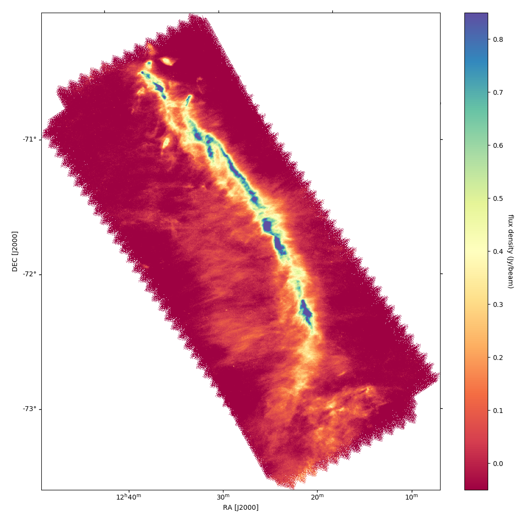
Musca is a prominent 6 pc long filamentary structure with a high aspect ratio at a distance of only 140-150 pc (Hacar et al. 2016; Cox et al. 2016; Kainulainen et al. 2016; Gaia Collaboration et al. 2018). It has a low average column density $N$, with $N$(max)$\sim$4-8 10²¹ cm^-2 (Bonne et al. 2020b), and shows only one protostellar source located at the northern end of the filament (Juvela et al. 2012; Machaieie et al. 2017). Furthermore, Herschel observations reveal a network of striations orthogonal to the filament, which are suggested to be indications of mass inflow along the magnetic field (Cox et al. 2016). Indication of continuous mass accretion from inflow towards the Musca filament was found by observed presence of low-velocity filament accretion shocks around the Musca filament (Bonne et al. 2020b). Hacar et al. (2016) conclude from individual ¹³CO and C¹⁸O pointings that the crest of the Musca filament is a single velocity coherent structure. It was proposed (Tritsis & Tassis 2018) that the Musca filament is only a sheet viewed edge-on, but our detailed study using APEX and SOFIA spectroscopic observations (Bonne et al. 2020a) showed that the data best fit with the concept that the crest of Musca is a dense ($n_{H_{2}}\sim$10⁴ cm^-3), cylindrical structure and not a low-density sheet and that the mass input for building up the crest is provided by large-scale flows but there is no evidence that this inflow appears in the form of striations. The striations are then only the result of gas compression by magnetosonic waves, which could fit with what was recently suggested by theoretical studies (Tritsis & Tassis 2016).

The Herschel SPIRE 250 $\mu$m data of Musca (Fig. 1) used in this paper are part of the Herschel Gould Belt Survey (André et al. 2010) and are published in (Cox et al. 2016). We use here the same dataset that was obtained in Parallel Mode at a sampling at 10Hz and at high speed (60^′′/s), and reduced using modified pipeline scripts of HIPE version 10. The resulting Level1 contexts for each scan direction (two maps were taken with orthogonal directions) were then combined using the ’naive’ map maker in the destriper module. The conversion of the maps into surface brightness (from Jy/beam into MJy/sr) was done using the beam-areas obtained from measurements of Neptune (March 2013). The zeroPointCorrection task was used to absolutly calibrate the maps using information from the Planck satellite. The angular resolution of the maps at 250 $\mu$m is 18^′′. We here use the 250 $\mu$m flux map for our studies and not the dust column density map used in (Cox et al. 2016; Bonne et al. 2020b, a) because the latter has only an angular resolution of 36^′′. The 250 $\mu$m map can be considered as a good proxy for the column density, however, in regions that are not strongly affected by stellar feedback (Miville-Deschênes et al. 2010) because it traces mostly cold dust that is mixed with the cold molecular gas.

3 Canonical and microcanonical approach to multifractality

A number of Galactic studies using continuum data or emission lines of atomic hydrogen or molecules showed that the Fourier power spectrum of the observed line intensity was well fitted by a power-law - at least over certain size scales - and which was commonly interpreted as a consequence of the scale-free and turbulent nature of the ISM (Scalo 1987; Green 1993; Elmegreen & Scalo 2004; Stutzki et al. 1998; Miville-Deschênes et al. 2010; Schneider et al. 2011; Robitaille et al. 2020). As mentioned since the introduction of the first phenomenological descriptions of hydrodynamic turbulence (Frisch 1995), the observed scale invariance suggests the existence of a energy cascade in which energy injected at large scales is transferred into smaller ones hence providing a natural explanation for the complex structure of the ISM at each scale. The Fourier power spectrum with its single descriptive parameter (the slope of the spectrum), however, turned out to be a too coarse descriptor to encode all turbulent and scale-free phenomena observed in the ISM and notably filamentary structures (Roy et al. 2015, 2019; Arzoumanian et al. 2019). The simplest models able to describe the partition of energy across the scales of a turbulent medium are monofractal: they rely on a single parameter, the fractal dimension, which characterizes the geometry of the sets between which the energy transfer is operated.

For modeling purposes in astronomy, monofractal signals can be generated using stochastic processes such as the fractional Brownian motion (fBm) (Mandelbrot & Ness 1968) and, more specifically, 2-dimensional fBMs (Heneghan et al. 1996; Stutzki et al. 1998; Robitaille et al. 2020). Such fBms are parametrized by their Hurst exponent which defines their monofractal properties. In (Khalil et al. 2006) a monofractal signature is found in atomic hydrogen data from the Canadian Galactic Plane Survey, while an anisotropic signature is also detected. The complex organization of the ISM can be fully described by the multifractal formalism which is as necessary in magneto-hydrodynamic turbulence as it is needed in hydrodynamic turbulence (Frisch 1995; Robitaille et al. 2020).

The multifractal formalism is already used in astronomy, e.g., in heliophysics turbulence (Movahed et al. 2006; McAteer et al. 2007; Salem et al. 2009; Kestener et al. 2010; Macek et al. 2014; Wu et al. 2015; Cadavid et al. 2016; Maruyama et al. 2017), the ISM (Elia et al. 2018), the large scale structure of the universe (Gaite 2007; Gaite & Domínguez 2007), galaxy mergers (De La Fuente Marcos & De La Fuente Marcos 2006), and gravitational waves detection (Eghdami et al. 2018). This formalism comes into two distinct presentations: canonical and microcanonical. The first one is the most popular (Arneodo et al. 1995); it includes the Wavelet Transform Modulus Maxima method (WTMM) (Arneodo et al. 1995; Turiel et al. 2006) and the cumulant approach (Brillinger 1994; Delour et al. 2001; Wendt et al. 2006; Ciuciu et al. 2008; Venugopal et al. 2006b). Microcanonical approaches where developed first in poorly accurate versions such as the counting box and histogram methods, then in an efficient geometrico-statistical formulation (Turiel et al. 2008) which we will use in this work. In the following, we review the most important aspects of the multifractal approach without being exhaustive.

In hydrodynamics or magneto-hydrodynamic turbulence, one observes, as explained before, a very complex partition of the energy according to the scale (She et al. 1990; Frisch 1995; Shivamoggi 2015) and it was understood that this complexity was an effect of intermittency, i.e., a consequence of the extremely complex geometrical organization, or partition, of the support of the energy at small scales. Observationally, this was supported by the detection of strong velocity-shears at sub-parsec scale (Falgarone, E. et al. 2009). Multifractal models were introduced to describe this intermittency because they allow to relate the fluctuations of a physical variable (such as the projection of velocity on a given fixed axis) to the complex geometry of the points where such a physical variable changes abruptly. First, we consider a fluid evolving in a two or three dimensional medium, and denote by ${\bf v}({\bf x})$ the velocity vector at a given point ${\bf x}$ inside the medium. One can then measure the values taken by ${\bf v}({\bf x})$ either in time at a fixed point ${\bf x}$ or at a fixed time at many different points ${\bf x}$. Experimentally, some decades ago, it was much more easier to measure the projection of the turbulent velocity field ${\bf v}$ in a specific fixed direction defined by a unitary vector ${\bf u}$ instead of the vector ${\bf v}({\bf x})$ itself. Nowadays, laser-mounted optical devices allow a direct measurement of the velocity vector field. Nevertheless, following the experimental setup described in Frisch (1995), measuring the velocity field in a fixed direction allows to evaluate the statistical moments

$$\langle\left|\left({\bf v}({\bf x}+{\bf r}{\bf u})-{\bf v}({\bf x})\right)\cdot\displaystyle{\bf u}\right|^{q}\rangle$$ (1)

of the turbulent velocity field ${\bf v}$; depending on the experimental setup, in equation 1 the averages $\langle\leavevmode\nobreak\ \cdot\leavevmode\nobreak\ \rangle$ can be computed either in time at a given point ${\bf x}$ or spatially over the domain. Then it was observed that the moments in equation 1 behaves as ${\bf r}^{\xi(q)}$ when ${\bf r}$ is inside a well defined interval of scale values $[{\bf r}_{1},{\bf r}_{2}]$ called the inertial range:

$$\langle\left|\left({\bf v}({\bf x}+{\bf r}{\bf u})-{\bf v}({\bf x})\right)\cdot\displaystyle{\bf u}\right|^{q}\rangle\sim{\bf r}^{\xi(q)}.$$ (2)

When $\xi(q)$ is a linear function of $q$ we are in the monofractal formalism. On the other hand, $\xi(q)$ is observed experimentally to be nonlinear in $q$ which means a multifractal behaviour. The nonlinearity of ${\xi(q)}$ as a function of $q$ is thus interpreted as a consequence of intermittency, it has a geometric origin and the link between statistics and geometry is as follows. Let us denote by ${\cal F}_{\bf h}$ the set of points ${\bf x}$ whose velocity increments, measured in the unitary direction ${\bf u}$ as before, behave as ${\bf r}^{\bf h}$ for a certain ${\bf h}$ i.e.

$${\cal F}_{\bf h}=\{{\bf x}\leavevmode\nobreak\ \mbox{s.t.}\leavevmode\nobreak\ \left|\left({\bf v}({\bf x}+{\bf r}{\bf u})-{\bf v}({\bf x})\right)\cdot\displaystyle{\bf u}\right|\sim{\bf r}^{\bf h}\leavevmode\nobreak\ \leavevmode\nobreak\ \mbox{when}\leavevmode\nobreak\ \leavevmode\nobreak\ {\bf r}\rightarrow 0\}.$$ (3)

These sets ${\cal F}_{\bf h}$ for small or even negative values of ${\bf h}$ feature a complex geometrical organization which is closely related to the nonlinear behavior of $\xi(q)$. To quantify how the geometry of the sets ${\cal F}_{\bf h}$ is related to the turbulent behavior of the velocity field, one can introduce a notion of dimension for these sets, called the Hausdorff fractal dimension (Falconer 1997), which is a positive real number describing the way they fill in the space. We will come back to this point in Sect. 3.3 but let us denote for the moment $D({\bf h})$ the Hausdorff fractal dimension of the sets ${\cal F}_{\bf h}$:

$$D({\bf h})=\dim_{H}({\cal F}_{\bf h}).$$ (4)

The link between geometrical complexity and statistical behavior is then given by the relation:

$$\xi(q)=\underset{{\bf h}>0}{\operatorname{inf}}(q{\bf h}+d-D({\bf h})),$$ (5)

where $d$ is the dimension of embedding space of the experiment ($d=2$ in 2D turbulence, $d=3$ in 3D turbulence), i.e. $\xi(q)$ appears as a Legendre transform. The mapping

$${\bf h}\mapsto D({\bf h})$$ (6)

is called the singularity spectrum of the velocity field. In the monofractal formalism, ${\xi(q)}$ is a linear function of $q$ and the mapping (6) reduces to a single point in the graph of $D({\bf h})$. In the multifractal formalism eq. (6) defines a distribution of fractal dimensions as a function of ${\bf h}$. In general $\displaystyle{\bf h}=\frac{\mbox{d}\xi}{\mbox{d}q}(q)$.

The notion applies of course to any signal $s({\bf x})$ or random process $(X_{t})_{t\geq 0}$ with values in $\mathbb{R}^{d}$ displaying a multiscale behaviour i.e. a nonlinear scaling of moments $\langle\|X(t)\|^{q}\rangle=c(q)t^{\xi(q)}$ for a nonlinear mapping $q\mapsto\xi(q)$, or to even more general multifractal random processes (Grahovac 2020). As we will see in Sect. 3.3, it also applies to measures. The singularity spectrum thus contains a lot of information on the statistics of turbulence but its computation is a fundamental problem of the multifractal formalism.

The intermittency of the velocity field, which is responsible of the observed scaling behavior and the partition of energy at different scales, has been the subject of a description in terms of random multiplicative cascades proposed by the Russian school (Kolmogorov 1941, 1962; Yaglom 1966; Novikov 1990, 1994). Denoting $(\delta v)_{{\bf r}}$ the longitudinal increments $\left|\left({\bf v}({\bf x}+{\bf r}{\bf u})-{\bf v}({\bf x})\right)\cdot\displaystyle{\bf u}\right|$, it was proposed to model the cascade through the probability distribution for $(\delta v)_{{\bf r}}$ (Castaing, B. 1996; Arneodo et al. 1998)

$${\cal P}_{(\delta v)_{{\bf r}_{1}}}=\displaystyle\int_{\mathbb{R}}G_{{\bf r}_{1}{\bf r}_{2}}(u)e^{-u}{\cal P}_{e^{-u}(\delta v)_{{\bf r}_{2}}}\,\mbox{d}u$$ (7)

which expresses the change in scales of the probability distribution depending on a kernel measure $G_{{\bf r}_{1}{\bf r}_{2}}$ (${\bf r}_{1}<{\bf r}_{2}$). For instance if $G_{{\bf r}_{1}{\bf r}_{2}}$ were a Dirac measure, then eq. 7 implies that ${\cal P}_{(\delta v)_{{\bf r}_{1}}}$ would have the same shape as ${\cal P}_{(\delta v)_{{\bf r}_{2}}}$ within a scaling factor in the velocity amplitudes. Equation 7 is satisfied if the kernel $G$ satisfies the convolution law (for each monotonic sequence of scales ${\bf r}_{1}<{\bf r}_{2}<\cdots<{\bf r}_{n}$)

$$G_{{\bf r}_{1}{\bf r}_{n}}=G_{{\bf r}_{1}{\bf r}_{2}}*\cdots*G_{{\bf r}_{n-1}{\bf r}_{n}}$$ (8)

which implies that the laws ${\cal P}_{(\delta v)_{{\bf r}}}$ are indefinitely divisible. In turn, this can be physically interpreted in the form of the multiplicative cascade.

3.1 $\log$-normal and $\log$-Poisson processes

Figure 2: Left: general form of the singularity spectrum $D({\bf h})$, Legendre transform of $\xi(q)$. See text for a definition of $D({\bf h})$, $\xi(q)$ and ${\cal F}_{\bf h}$. Middle and right: singularity spectrum of a $\log$-normal process with $d=2$, ${\bf h}_{m}=0$ and $\sigma_{\bf h}=0.5$ (middle panel) and of a $\log$-Poisson process with $d=2$, $D_{\min}=1.07$ and ${\bf h}_{\min}=-0.5$ (right panel).

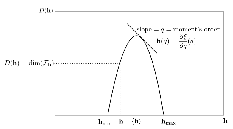
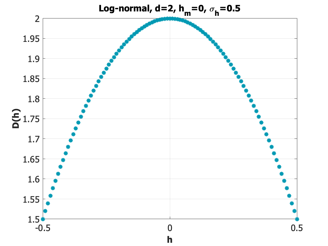
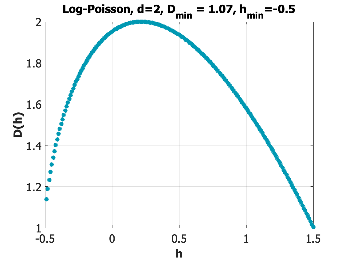
There are only few cases for which a singularity spectrum can be computed exactly. We give here two examples, well-known for their physical interpretation, that will also play a key role in this study: the $\log$-normal and the $\log$-Poisson processes.

The energy cascading model for intermittency in a turbulent medium mentioned previously implies a multiplicative form for the energy dissipation rate $\dot{\varepsilon}({\bf x})$ (Vazquez-Semadeni 1994). Indeed, an initial volume of space is divided into 8 equal cubes of size half the size of the initial volume; the energy dissipation rate is then multiplied by 8 random variables, equally distributed. When this scheme is recursively repeated, the field $\dot{\varepsilon}({\bf x})$ at a given scale does have a multiplicative form. Its logarithm is then a sum of random variables and, under the hypotheses of the central limit theorem, the energy dissipation rate can be approximated by a $\log$-normal process. In that case, the space intermittency comes from the existence of a large number of regions with nearly equal dissipation rates. The $\log$-normal model was introduced by N. Kolmogorov (Kolmogorov 1962).

There are, however, different intermittency models which depend on various assumptions about the energy dissipation rate (Hopkins 2013). In Gledzer et al. (1996) an energy cascade model of intermittency is introduced, involving rare localized regions of both large and weak energy dissipation areas, in the spirit of (She & Leveque 1994), leading to $\log$-Poisson statistics. It is a model with dissipatively active and passive localized regions, allowing the existence of ”holes of dissipation”; $\log$-Poisson processes are particularly interesting in this context for their potential ability to describe distribution of filaments, as we will see in this work.

The singularity spectrum ${\bf h}\mapsto D({\bf h})$ can be computed in a closed form in the case of $\log$-normal and $\log$-Poisson processes. Precisely:

• A $\log$-normal process in $\mathbb{R}^{d}$ has a parabolic singularity spectrum

  $$D({\bf h})=\displaystyle d-\frac{1}{2}\left(\frac{{\bf h}-{\bf h}_{m}}{\sigma_{{\bf h}}}\right)^{2}$$ (9)

  with $\xi(q)={\bf h}_{m}q-\displaystyle\frac{1}{2}\sigma_{{\bf h}}q^{2}$, ${\bf h}_{m}$: mean singularity, $\sigma_{{\bf h}}$: singularity dispersion.

• A $\log$-Poisson process in $\mathbb{R}^{d}$ is a translationally invariant indefinitely divisible process with a singularity spectrum given by

  $$D({\bf h})=D_{\min}+(d-D_{\min})\omega({\bf h})(1-\log\omega({\bf h}))$$ (10)

  with $\omega({\bf h})=\displaystyle\frac{{\bf h}-{\bf h}_{\min}}{(d-D_{\min})(-\log\beta)}$, ${\bf h}_{\min}$: minimum value of singularities, $D_{\min}$: associated dimension of set ${\cal F}_{{\bf h}_{\min}}$ and $\beta$ is the dissipation parameter ($0<\beta<1$): $\beta=\displaystyle 1+\frac{{\bf h}_{\min}}{d-D_{\min}}$. Accordingly, $\xi(q)={\bf h}_{\min}q+(d-D_{\min})(1-\beta^{q})$.

In general, for a wide class of processes, the singularity spectrum $D({\bf h})$, being the Legendre transform of $\xi(q)$, has a concave shape, shown the left panel of Fig. 2. The same figure displays the singularity spectra of typical $\log$-normal processes (middle panel), and $\log$-Poisson processes (right panel).

A $\log$-normal singularity spectrum, being parabolic, is symmetric, while a $\log$-Poisson process has a non-symmetric singularity spectrum. The lack of symmetry is a strong indication of very different dynamic properties compared to those described by a $\log$-normal model. In this work we focus on the $\log$-normal and $\log$-Poisson processes because they are associated to geometrical models. It must be noted however, that there are other models among them the $\log$-$\alpha$-stable which also has also a non-symmetric spectrum (Schmitt & Huang 2016).

3.2 Existing computational approaches

In this subsection we summarize previous works done in astronomy which made use of the multifractal approach. We recapitulate previous introductions given in Elia et al. (2018) and Khalil et al. (2006); McAteer et al. (2007); Salem et al. (2009); Kestener et al. (2010); Macek et al. (2014); Robitaille et al. (2020), and combine those with more fundamental presentations given in Arneodo et al. (1995); Turiel et al. (2008) that describe general signal processing approaches.

Equation (3) defines the scaling exponents $\bf{h}$ from the true turbulent velocity field ${\bf v}({\bf x})$, which is not directly accessible either in astronomy, or in many other geophysical sciences. The basic information from which numerical computations are performed is one or more observational maps, which constitute an original signal denoted $s$ in the following. Consequently, in signal processing, the multifractal formalism consists in defining and computing singularity exponents h(x) and other characteristics like the singularity spectrum from the data in $s$. This is done by considering, from the data in $s$, general positive measures, denoted $\mu$ instead of the unknown velocity field ${\bf v}({\bf x})$. These can be for instance probability measures built out of the signal, or some kind of additive quantity defined in the domain of the signal $s$.

If $\mu$ is a positive measure, and if ${\cal B}({\bf x},{\bf r})$ is a ball centered at point ${\bf x}$ and of radius ${\bf r}$ in the signal’s domain, we can evaluate the measure of that ball, $\mu({\cal B}({\bf x},{\bf r}))$ and, since the measure is supposed to be positive, one can consider the limit

$${\bf h}({\bf x})=\displaystyle\lim_{{\bf r}\rightarrow 0}\displaystyle\frac{\log\mu({\cal B}({\bf x},{\bf r}))}{\log({\bf r})}$$ (11)

called the singularity exponent ${\bf h}({\bf x})$ of $\mu$ at ${\bf x}$ (Arneodo et al. 1995; Venugopal et al. 2006a; Turiel et al. 2008). The singularity exponent ${\bf h}({\bf x})$ appears as a power law exponent in the limiting measures of the balls:

$$\mu({\cal B}({\bf x},{\bf r}))\sim{\bf r}^{{\bf h}({\bf x})}$$ (12)

when ${\bf r}\rightarrow 0$. A singularity exponent ${\bf h}({\bf x})$ encodes a limiting scaling information at every point ${\bf x}$. It is a pointwise generalization of other scaling parameters often used by astrophysicists and defined globally such as the power law of a power spectrum or the $\Delta$-variance (Ossenkopf et al. 2008). If the singularity exponents ${\bf h}({\bf x})$ can be computed at every point ${\bf x}$ in the signal’s domain, then we can generalize equation 3 and define the sets

$${\cal F}_{\bf h}=\{\leavevmode\nobreak\ {\bf x}\leavevmode\nobreak\ |\leavevmode\nobreak\ {\bf h}({\bf x})={\bf h}\leavevmode\nobreak\ \}.$$ (13)

Like in equation 4, the complex organization of the sets ${\cal F}_{\bf h}$ is measured by their fractal dimension. This implies that if we cover the support of the measure $\mu$ with balls of size ${\bf r}$, the ”histogram” $N_{\bf h}(\bf r)$, or number of such balls that scale as ${\bf r}^{{\bf h}}$ for a given ${\bf h}$ behaves like

$$N_{\bf h}({\bf r})\sim{\bf r}^{-D({\bf h})}$$ (14)

(see (Arneodo et al. 1995)). Hence, the singularity spectrum ${\bf h}\mapsto D({\bf h})$ is a distribution which represents the limiting behavior of the histograms $N_{\bf h}({\bf r})$ when ${\bf r}\rightarrow 0$; it is one of the fundamental tools to study complex and turbulent signals. Obviously, the main problem in the analysis of observational maps in astronomy is to be able to compute the singularity spectrum for the whole map or parts of it.

The most direct approach, which consists in estimating the slope of $\log\mu({\cal B}({\bf x},{\bf r})$ vs. $\log{\bf r}$ for various ${\bf r}$ (”box-counting method”), is known to be inefficient and can potentially lead to errors (Arneodo et al. 1995; Chappell & Scalo 2001). In (Elia et al. 2018) the authors make use of the generalized fractal dimensions $D_{q}$: the support of the signal’s domain is covered with boxes ${\cal B}({\bf x}_{i},{\bf r})$ of size ${\bf r}$ ($1\leq i\leq N({\bf r})$), and $\mu_{i}({\bf r})$ is defined to be the proportion of signal values inside a ball ${\cal B}({\bf x}_{i},{\bf r})$. In this case the measure $\mu$ reduces to consider the signal as a probability distribution. Then a partition function is defined:

$$Z(q,{\bf r})=\displaystyle\sum_{i=1}^{N({\bf r})}\mu_{i}({\bf r})^{q}.$$ (15)

In the limit ${\bf r}\rightarrow 0$ one has, just like in equation 2:

$$Z(q,{\bf r})\sim{\bf r}^{\tau(q)}$$ (16)

and the generalized dimensions are defined as

$$D_{q}=\displaystyle\frac{\tau(q)}{q-1}.$$ (17)

Some of the quantities $D_{q}$ can be interpreted: $D_{0}$ is the box dimension of the support of $\mu$, i.e., the dimension of the signal’s support as defined in Elia et al. (2018), $D_{1}$ is the ”information dimension”, and for $q\geq 2$, $D_{q}$ encodes the scaling of correlation integrals. In Arneodo et al. (1995) it is shown that the relation between $\tau(q)=(q-1)D_{q}$ and the singularity spectrum $D({\bf h})$ is as follows:

$$\tau(q)=\underset{{\bf h}}{\operatorname{min}}(q{\bf h}-D({\bf h}))$$ (18)

i.e., a Legendre transform. This leads to an interpretation of the multifractal formalism with thermodynamics: $q$ is identified with a Boltzmann inverse temperature and the multifractal formalism allows the study of the self-similarity phases of the measure $\mu$. The limit ${\bf r}\rightarrow 0$ is the thermodynamic limit at infinite volume ($V=\log\displaystyle\frac{1}{\bf r}$) and ${\bf h}_{i}=\displaystyle\frac{\log\mu_{i}}{\log{\bf r}}=\frac{-\log\mu_{i}}{\log\left(\frac{1}{\bf r}\right)}$ corresponds to $E_{i}$, the energy per unit volume of miscrostate $i$. The partition function $Z(q,{\bf r})$ is rewritten in its usual form:

$$Z(q,{\bf r})=\displaystyle\sum_{i}e^{-qE_{i}}.$$ (19)

In this context, the singularity spectrum ${\bf h}\mapsto D({\bf h})$ is the entropy per unit volume, so that the computation of the singularity spectrum is equivalent to the computation of the entropy per internal energy in a large multi-body system. This is one microcanonical formulation of the multifractal formalism, which is correct only in the thermodynamic limit, because it corresponds to microcanonical ensembles of thermodynamics. It can be implemented numerically through the box-counting or the histogram methods. This is the approach used in Chhabra et al. (1989); Chappell & Scalo (2001); Elia et al. (2018), and also in Movahed et al. (2006) with detrending in the context of solar data. This approach however, gives poor results due to severe finite size effects (Arneodo et al. 1995). Very importantly, an essential criterion for verifying the quality of the results obtained with this or any other multifractal approach is to test the results on several rescaled versions of the same signal. The singularity spectrum, for example, must be the same for different scales by the very definition of scale invariance. This is not the case with the box-counting implementation, as we will demonstrate in Sect. 4.

To cope with the difficulties of the microcanonical approach, canonical formulations have been introduced in the literature. They consist in evaluating the ${\bf h}$ values and $D({\bf h})$ as averages among many realizations, i.e., in a canonical ensemble. This approach supposes the availability of many realizations of a same system. The canonical approach to multifractal formalism is presently the most used when grand ensembles of signal’s realizations are available. The most advanced canonical numerical implementations include: the Wavelet Transform Maximum Modulus (WTMM) technique (see (Arneodo et al. 1995; Venugopal et al. 2006a; Khalil et al. 2006) for a detailed exposition), the cumulant analysis method, which we use in this work for analyzing $\log$-correlations (Venugopal et al. 2006a), the wavelet leaders technique (Serrano & Figliola 2009), and the multifractal detrended fluctuation analysis (MDFA) (Kantelhardt et al. 2002).

As an example, the WTMM methodology applied on a signal $s({\bf x})$ from an observational map (so that ${\bf x}$ refers to the spatial coordinates in the signal), makes use of an analyzing wavelet $\psi$ with sufficient vanishing moments to filter out spurious long-range correlations, and the wavelet-projected signal ${\cal T}_{\psi}({\bf x},{\bf r})$ evaluated at position ${\bf x}$ and scale ${\bf r}$, a suitably chosen $q$th order partition function $Z(q,{\bf r})$ built out of ${\cal T}_{\psi}$ so that $Z(q,{\bf r})\sim{\bf r}^{\tau(q)}$ when ${\bf r}\rightarrow 0$ (see Venugopal et al. (2006a) for computationally effective choices of partition functions). The singularity spectrum is recovered as $D({\bf h})=\underset{q}{\operatorname{min}}(q{\bf h}-\tau(q))$. This supposes the correct evaluation of $\tau(q)$ through $\log$-$\log$ regression with large amounts of data coming from ensembles of realizations of the signal.

In the study of the ISM, in most of the cases grand ensembles of observational maps of the same cloud are not available; this is the reason why (Elia et al. 2018) favors a microcanonical computational approach over the canonical formulations. Using box-counting or histogram methods, however, do not produce satisfactory evaluations of the singularity spectrum. In this work, we develop an alternative and much more reliable implementation of the microcanonical approach, introduced in the next section.

3.3 Singularity spectrum from ”microstates”

One major goal of the microcanonical multifractal formalism is to evaluate precisely the quantities ${\bf h}({\bf x})$ for a well defined measure $\mu$ and to derive the singularity spectrum ${\bf h}\mapsto D({\bf h})$ in order to obtain information on the statistics of a complex and turbulent signal. We present in this section and Appendix A the

determination of the singularity spectrum and the singularity exponents in a microcanonical formulation based on the theory of predictability in complex systems (Turiel et al. 2008), which overcomes the drawbacks of the box-counting and histogram methods.

In the case of observational maps in astronomy, but also in the analysis of general turbulence data, scaling is valid only within a certain inertial range of scales (Sect. 3) and we have to define a measure from a finite set of discrete acquisitions values in the map. Hence, we follow the exposition of the multifractal ansatz in the physics of disordered systems, which allows for a rigorous presentation of the multifractal formalism in the case of discrete signals (Fyodorov 2010; Fyodorov et al. 2012). First, we have to define a measure from the data of an observational map. In previous works Chhabra et al. (1989); Chappell & Scalo (2001); Elia et al. (2018) the measure is often defined from the the signal $s$ itself. Following Turiel et al. (2008), it turns out that better accuracy is obtained when starting from discrete gradient information. Consequently we consider an inertial range in the image domain $[{\bf r}_{1},{\bf r}_{2}]$ which we identify for convenience with the unit square $[0,1]^{2}$. We define a collection of refined lattice points as follows: for each $n\in\mathbb{N}$, let us consider the set $\Omega_{n}$ of points whose coordinates are integer multiples of $2^{-n}$ inside the unit square. We get an increasing sequence $\Omega_{0}\subset\Omega_{1}\subset\cdots\subset\Omega_{n}\subset\cdots$ of lattice points as shown in Fig. 3.

Figure 3: Increasing sequence of lattice nets $\Omega_{0}\subset\Omega_{1}\subset\cdots\subset\Omega_{n}\subset\cdots$ inside the unit square.

For each ${\bf x}\in\Omega_{n}$ we define a finite set of neighboring points ${\cal V}_{n}({\bf x})$ as shown in Fig. 4.

Figure 4: Discrete neighborhood sets ${\cal V}_{n}({\bf x})$ at scale $2^{-n}$ around point ${\bf x}$.

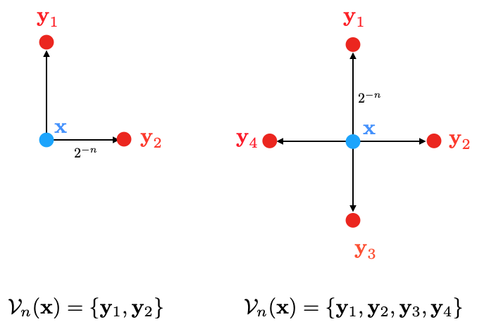
If ${\bf x}\in\Omega_{n}$, we have the information of the signal data $s({\bf x})$ at point ${\bf x}$ together with the discrete gradient’s norms determined by the differences $D({\bf x},{\bf y})=\displaystyle\frac{|s({\bf x})-s({\bf y})|}{\|{\bf x}-{\bf y}\|}$, with ${\bf y}\in{\cal V}_{n}({\bf x})$ of vicinity points around ${\bf x}$ at scale $2^{-n}$. We define a measure $\mu_{n}$ at that scale $2^{-n}$ from the discrete gradient information data. The exact definitions are given in Appendix A, and $\mu_{n}$ is seen as a ”gradient measure” associated to the observational map data at scale $2^{-n}$, which means that the $\mu_{n}$-measure of a ball is the sum of discrete gradient’s norms information inside that ball.

The application of the multifractal formalism to the signal $s$ and its associated measure $\mu_{n}$ is valid only if the measure $\mu_{n}$ satisfies the scaling hypothesis shown in equation 36. In canonical implementations of the multifractal formalism, checking the scaling is a necessary first step before applying the numerical tools, and is generally done by $\log$-regression performed on the chosen partition functions. In existing microcanonical implementations such as in Elia et al. (2018), the scaling is shown only for output simulations of fractional Brownian motions realizations. In Sect. 5.3 we will make use of the 2D structure function methodology (Renosh et al. 2015)) to check the scaling of analyzed data.

The key idea in a computation of the singularity exponents in a microcanonical setting based on predictability is to relate the quantities ${\bf h}({\bf x})$ to the signal’s reconstruction. In physical signals, the set of possible values taken by ${\bf h}({\bf x})$ is bounded, and the lowest singularity exponents’ value ${\bf h}_{\infty}=\min\{{\bf h}({\bf x})\}$ corresponds to the sharpest transitions in a signal according to equation 12. The points ${\bf x}$ such that ${\bf h}({\bf x})={\bf h}_{\infty}$ form a particular subset ${\cal F}_{\infty}$ in the signal’s domain, of fractal nature, encoding the strongest transitions: in a 2D signal, ${\cal F}_{\infty}$ encodes the strongest edges, while the other sets ${\cal F}_{\bf h}$ correspond to more smoother edges and transitions as ${\bf h}$ increases. Under the assumption that ${\cal F}_{\infty}$ coincides with the set of most unpredictable points (in the sense of complex systems theory), it can be shown that the computation of ${\bf h}({\bf x})$ at scale $2^{-n}$ involves only immediate neighboring points around ${\bf x}$. When these intuitive considerations are expressed rigorously into a more mathematical manner, as shown in Appendix B, we arrive to a computation of the singularity exponents ${\bf h}({\bf x})$ using a correlation measure denoted ${\cal H}$ in Appendix B which can be evaluated locally around any point ${\bf x}$ in the signal domain’s, leading to equations 43 and 45 which we use as our fundamental methodology to compute the singularity exponents in a microcanonical formulation.

4 Experimental comparison of microcanonical methodologies: scale invariance

In this section, we test the validity of the scaling hypothesis eq. 36 by comparing the singularity spectra computed in a microcanonical formulation of the multifractal formalism using the two approaches mentioned previously: first, an enhanced version of the counting-box method presented in Sect. 3.2 called the gradient modulus wavelet projection method detailed in (Turiel et al. 2006) and second, the method explained in Sect. 3.3. The experiment is performed on the Musca Herschel 250 $\mu$m observational map described in more detail in Sect. 2.

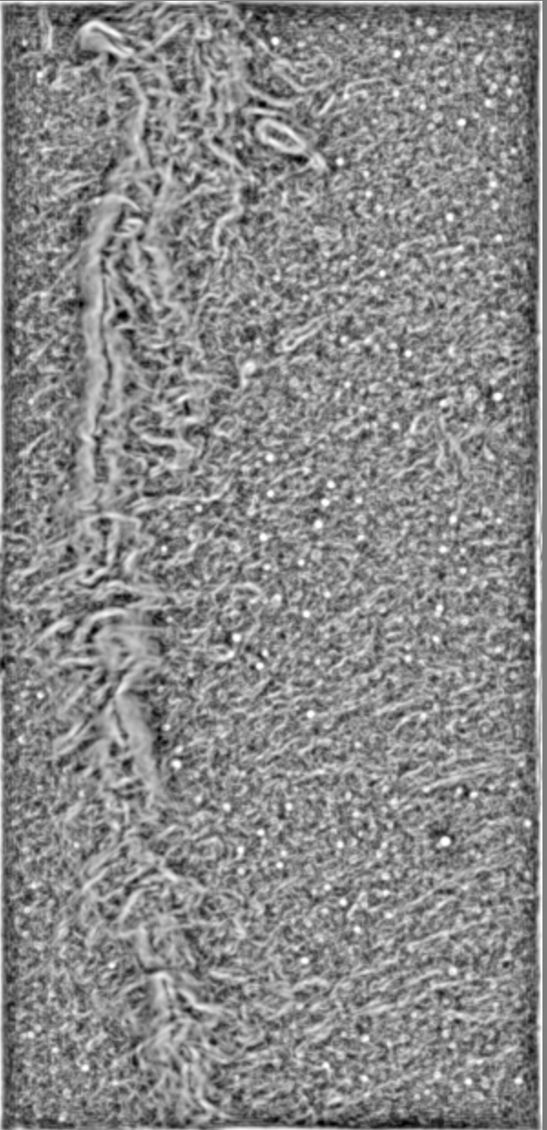
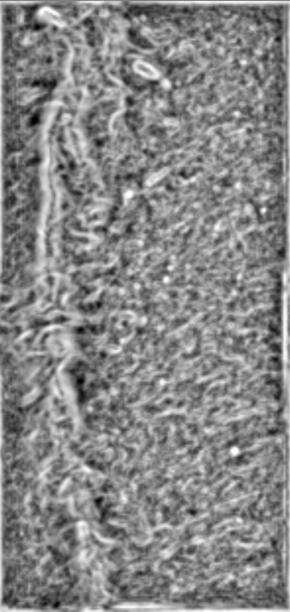
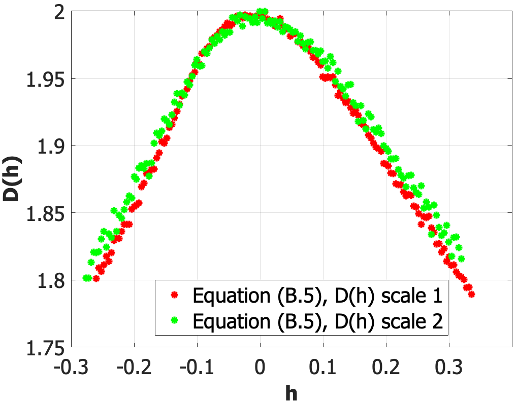
Scale invariance eq. 36 implies that singularity spectra computed from two scaled versions of an original observational map must coincide. Consequently, we will perform the following experiment: we take the Musca map, generate out of it two downscaled versions of the map, compute the singularity spectrum with either method on the two downscaled versions of the map (see below), and check if the resulting spectra coincide.

Figure 5: Top row, from left to right: visualization of the singularity exponents computed through $\log$-regression using a Lorentz wavelet of order 3 on the Musca 250 $\mu$m Herschel flux map presented in Sect. 2. Algorithm used to compute the singularity exponents: gradient modulus wavelet projection method. The two images correspond to two consecutive downscaled wavelet projections of the original signal using a discrete wavelet projection. Bottom: the resulting mappings ${\bf h}\mapsto D({\bf h})$ using the singularity exponents computed on the two consecutive scales (red: half scale of the original Musca 250$\mu$m Herschel flux map, green: 1/4 scale of original Musca 250$\mu$m Herschel flux map). We observe that, inside the domain corresponding to ${\bf h}\leq 0$, the two mappings do not coincide. Consequently, the $\log$-regression method for computing the singularity exponents provide poor result in this case.

Figure 6: Top row, from left to right: visualisation of the singularity exponents computed with the local correlation measure described in equations 45 and 43 on the Musca 250 $\mu$m Herschel flux map presented in Sect. 2. The two images correspond to two consecutive downscaled wavelet projections of the original signal using a discrete wavelet projection. Bottom: the resulting mappings ${\bf h}\mapsto D({\bf h})$ using the singularity exponents computed on the two consecutive scales (red: half scale of the original Musca Herschel map, green: 1/4 scale of original Musca Herschel map). We observe that the two mappings coincide much better than with the previously exponents computed from $\log$-regression and displayed in Fig. 5. Consequently, the local correlation measure algorithm exhibits the scaling in a much better way.

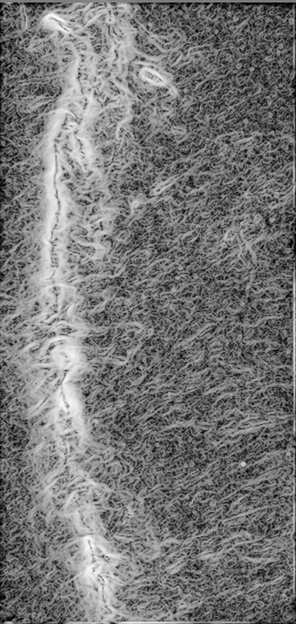
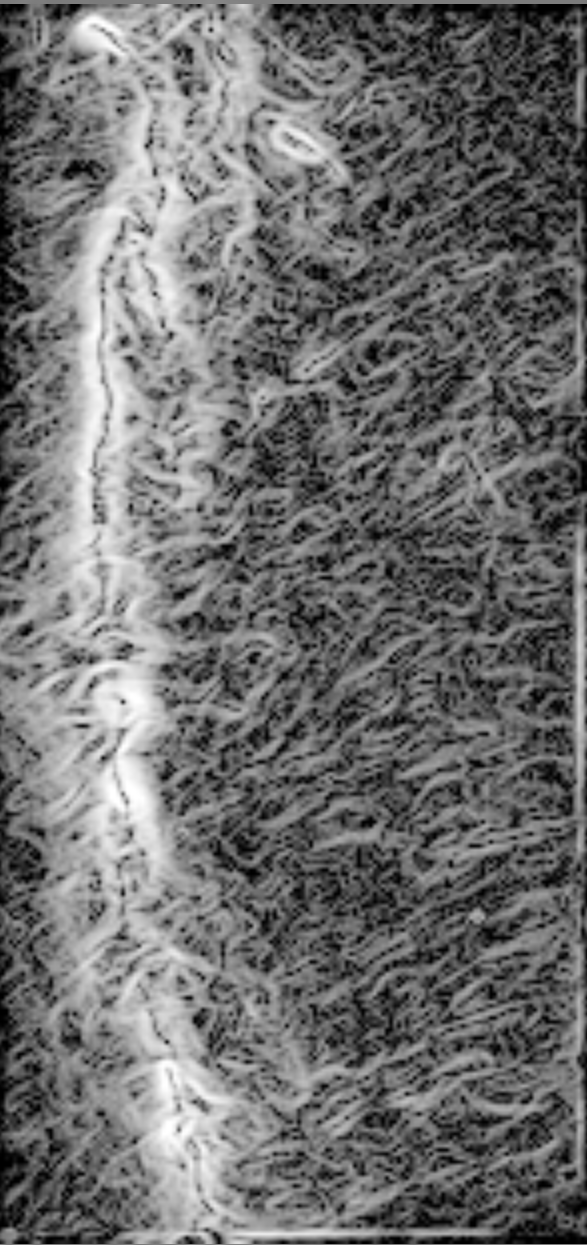
4.1 Gradient modulus wavelet projection method

The algorithm is described in detail in (Turiel et al. 2006). It is an enhanced counting-box method which allows for the computation of the singularity exponents ${\bf h}({\bf x})$ and the singularity spectrum ${\bf h}\mapsto D({\bf h})$ through a $\log$-regression performed, not directly on the scaling hypothesis eq. 36 but rather over wavelet projections of the measure for better computational accuracy. This approach is allowed because if a measure $\mu$ scales with singularity exponents ${\bf h}({\bf x})$, as in equation 36, wavelet projections of $\mu$ scale with the same exponents ${\bf h}({\bf x})$ as long as the analyzing wavelet has $n$ vanishing moments with $n>{\bf h}({\bf x})$ (Venugopal et al. 2006a; Turiel et al. 2008): if ${\bf r}>0$ is a scale, $\mu$ a measure on $\mathbb{R}^{2}$, $\psi$ a real wavelet, and $\lambda_{\bf r}$ the measure $\displaystyle\frac{1}{\bf r}\psi\left(\frac{-{\bf x}}{\bf r}\right)\,\mbox{d}{\bf x}$, the wavelet projection of $\mu$ at scale ${\bf r}$ is another measure noted ${\cal T}_{\psi}(\mu,{\bf r})$ which is the convolution of the measures $\mu$ and $\lambda_{\bf r}$:

$${\cal T}_{\psi}(\mu,{\bf r})=\lambda_{\bf r}*\mu.$$ (20)

If $\mu$ possesses a density, then ${\cal T}_{\psi}(\mu,{\bf r})$ has a density given by the usual continuous wavelet transform of the original density with mother wavelet $\psi$. The measure $\mu_{n}$ considered here is the one defined by eq. 28 with the neighboring set ${\cal V}_{n}({\bf x})$, corresponding to the left part of Fig. 4 (2 neighboring points). To compute the singularity exponents, we take as an analyzing wavelet a $\beta$-Lorentzian defined by

$$L_{\beta}({\bf x})=\displaystyle\frac{1}{(1+\|{\bf x}\|^{2})^{\beta}}$$ (21)

with $\beta=3$, with its support scaled to adapt to the signal Nyquist frequency. The $\log$-regression is performed over 30 scales.

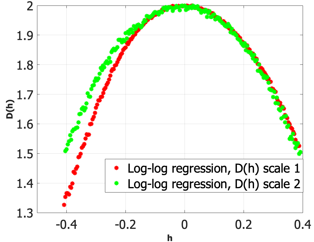
To check the scaling of the measure we downscale the original signal on two consecutive scales less than the original signal maximal resolution using a standard discrete wavelet transform defined by the reverse bi-orthogonal projection of order 4.4. Then, for each of these two downscaled wavelet projections, we compute the singularity exponents through $\log$-regression with the Lorenztian wavelet, as explained previously, to get two scalar fields of singularity exponents ${\bf h}({\bf x})$ at the two consecutive resolutions. From each of these scalar fields, we compute a mapping ${\bf h}\mapsto D({\bf h})$ using eq. 38: if the measure is scale invariant and if the singularity exponents are correctly computed, then the two mappings corresponding to each resolution should be coincident. We show the result of the $\log$-regression in Fig. 5. We observe in the figure that, inside the most informative part of the mapping, corresponding to ${\bf h}\leq 0$, the two mappings do not coincide. Consequently, the $\log$-regression method for computing the singularity exponents provide poor result in this case and the quantities computed through $\log$-regression do not show the scaling of the measure.

4.2 Local correlation measure of section 3.3.

In Fig. 6, we reiterate the previous experiment on the Musca 250 $\mu$m Herschel map, this time with the singularity exponents computed using eqs.  45 and 43. The resulting maps ${\bf h}\mapsto D({\bf h})$ reveal much more satisfactorily the scaling behavior of the measure because they coincide very well for the two consecutive scales over the range of singular values. This agreement is much stronger than the one of the exponents previously computed from $\log$-regression and displayed in Fig. 5. Consequently, the local correlation measure algorithm exhibits the scaling in a much better way. Note also that the resulting graphs differ notably from the ones computed using $\log$-regression and shown in the bottom of Fig. 5: they are much less ”parabolic”. It becomes obvious that the $\log$-regression method (gradient modulus wavelet projection algorithm) tends to produce singularity spectra of the $\log$-normal type in that case.

Figure 7: Map of the singularity exponents computed on filtered Musca 250 $\mu$m data. The image is a zoom of the singularity map over the central part of the Musca observation map, to better show how the singularity exponents reflect the complex distribution of filamentary coherent structures.

5 Application to the Musca observation map. Sparse filtering. Determination of the inertial range.

5.1 Map of the singularity exponents

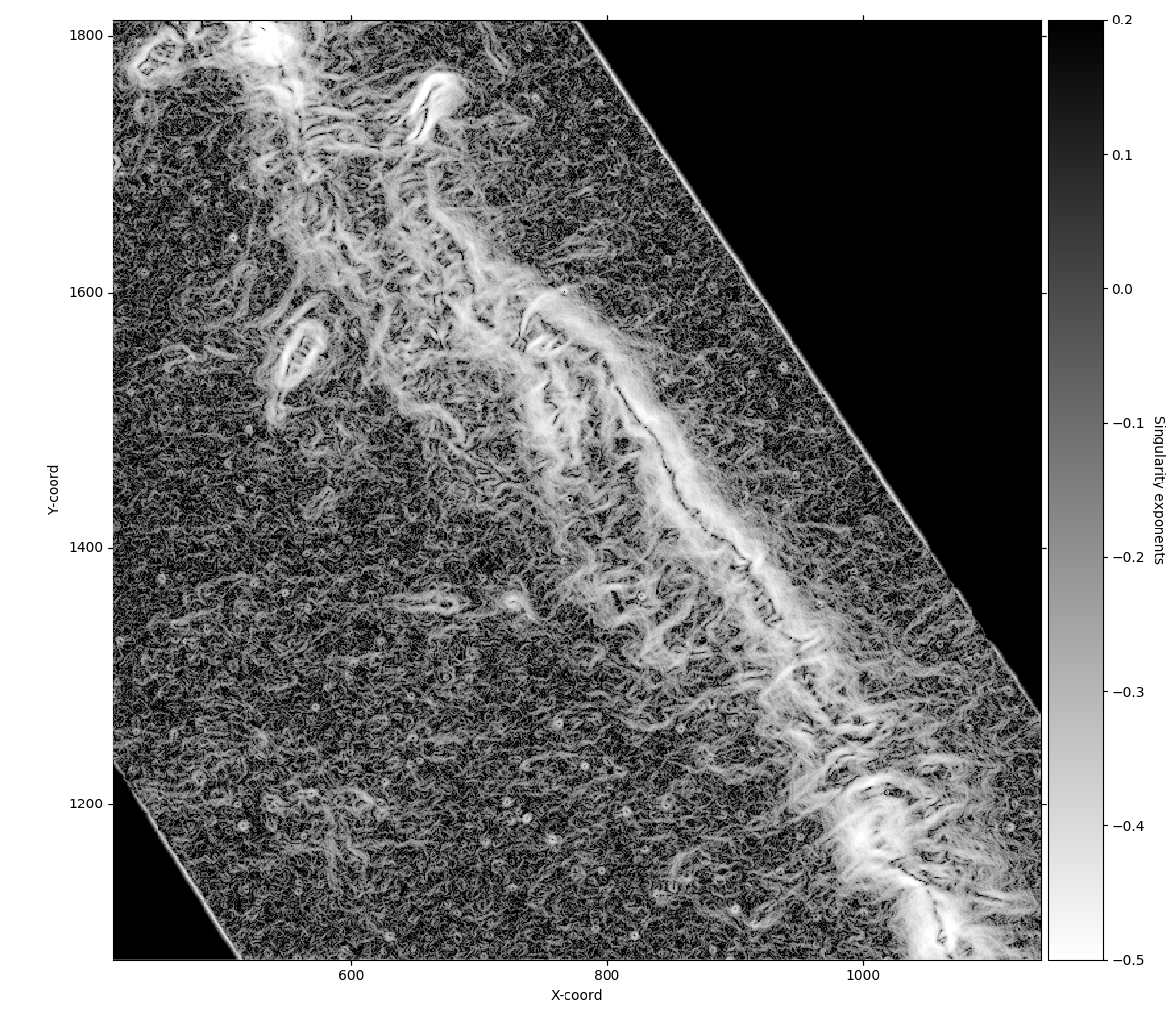
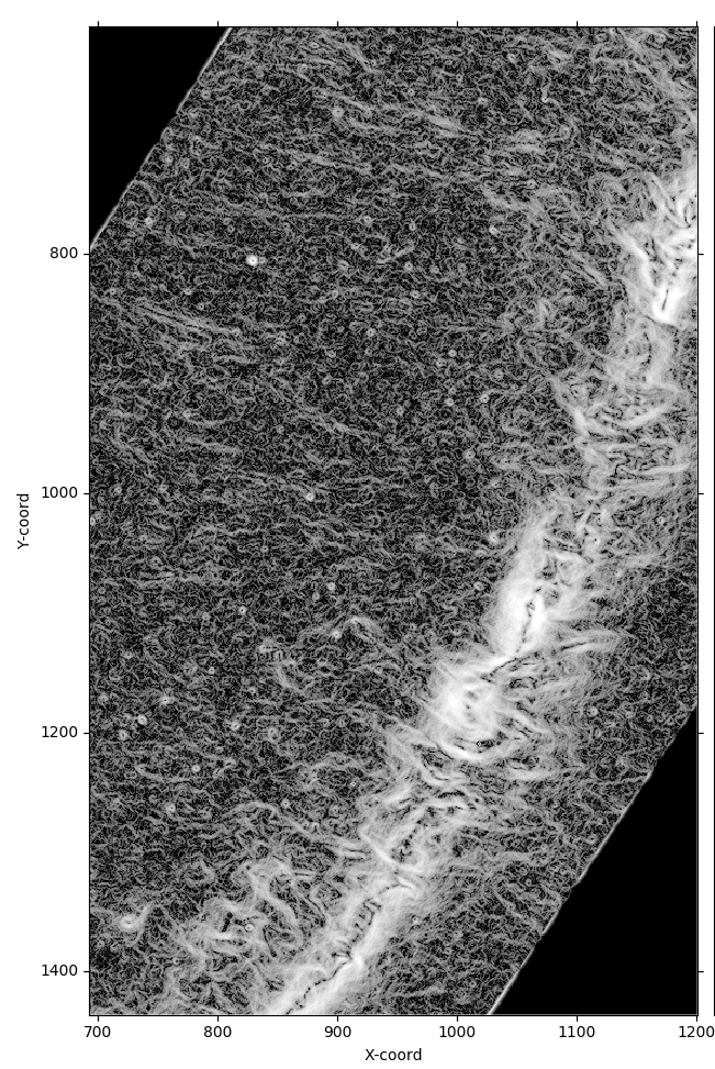
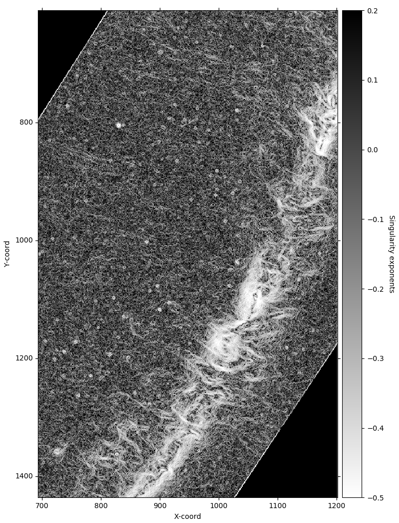
In Sect. 3 we introduced the multifractal formalism through the analysis of intermittency in the velocity field as this is the usual presentation in the turbulence literature. In this study, the analysis is done on thermal continuum emission using the discrete gradient measures introduced in Sect. 3.3. In Fig. 7 we display the singularity exponents ${\bf h}({\bf x})$ on the Herschel 250 $\mu$m map, computed using the local correlation measure defined by eqs. 45 and 43. The computation has been done on a filtered version of the map, described in Sect. 5.2, to eliminate some background noise. As we will see in the following, background noise elimination is performed not only for better visualization, but also to compute more precise singularity spectra. The wedge used in the figure is such that most negative singularity exponents are brighter. We can see how the singularity exponents trace the transitions in the signal, particularly along the filamentary structures, which are very well rendered by negative values of ${\bf h}({\bf x})$. Note also the thin dark region along the crest of the main filament: it follows a generatrix-like curve of a cylindrical structure, along which the flux appears constant. We observe the same phenomenon in MHD simulations, see middle picture of Fig. 17. In the case of the Musca cloud, however, a close inspection of the crest shows that this thin dark region is filled with small elongated structures perpendicular to the crest, making the picture even more complex. In addition, there are small circular features distributed all over the map that are most likely background galaxies that were not eliminated.

5.2 Sparse filtering of an observational map

Figure 8: Visualisation of the filtering (computed with $\lambda=0.7$) zoomed in the central part of the Musca 250 $\mu$m map. The level was chosen to emphasize low values. The left panel shows the filtered data and the right one the unfiltered data. The positive effect of the filtering on the flux density data becomes obvious. The visualisation done on the singularity exponents, displayed in Fig. 9, demonstrates the importance of the filtering on filamentary structures, which are of low fractal dimension.

Figure 9: Illustration of background noise elimination and enhancement of the filamentary structures in the Musca 250 $\mu$m map by edge-aware nonlinear filtering while promoting a signal’s gradients sparsity with $L^{1}$ norm. The images show the singularity exponents of a region in Musca that is rich in filamentary structures. The right panel displays the singularity exponents derived from the non-filtered original map, while the left panel shows the singularity exponents after filtering the map with $\lambda=0.7$ (eq. (1). The same greyscale wedge is used for both images.

Figure 10: Visualisation of the noise eliminated by the edge-aware noise filtering: the data displayed is $s-s_{f}$ in the same area as shown in figure 9.

Figure 11: Singularity spectrum of the Musca 250 $\mu$m Herschel map, computed with and without edge-aware filtering. The orange curve shows the singularity spectrum computed on raw non-filtered data while the blue curve displays the singularity spectrum computed on edge-aware filtered data using the filtering introduced in Sect. 5.2 with parameter $\lambda=0.7$. The horizontal axis gives the ${\bf h}$-values of the scaling exponents, the vertical axis the fractal dimension $D({\bf h})=\dim({\cal F}_{{\bf h}})$ (see Sect. 3.3). First, it becomes obvious that the part of the spectrum corresponding to ${\bf h}\leq 0$, i.e. the strongest transitions, is not accurately computed on the nonfiltered data, the presence of the background noise leads to an overestimation of the multifractal spectrum. Second, the slope of the right part of the graph is poorly evaluated in the presence of noise. As a result, the singularity spectrum computed on the filtered observation map is less symetrical w.r.t. the vertical axis ${\bf h}=0$.

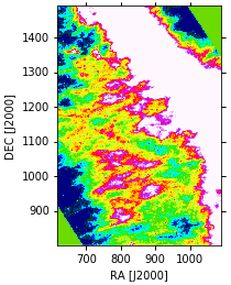
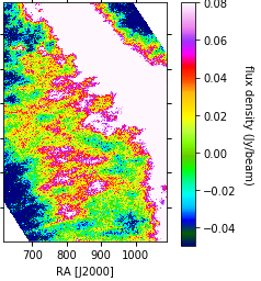
The Musca Herschel 250 $\mu$m flux map contains point-like sources, which are mostly galaxies, and the cosmic infrared background (CIB) and the cosmic microwave background (Padoan et al. 2001; Robitaille et al. 2019), which have isotropic low amplitude values very close to those of low scale filamentary structures. As a consequence, eliminating this ’noise’ is of primary importance in the multifractal analysis of the Musca gas. One possible method, presented in Robitaille et al. (2019), makes use of a filtering algorithm aiming at separating (and reconstructing) the large space-filling monofractal content of an image from the coherent structures which have a multifractal nature. This technique applies a threshold on the probability distribution function (PDF) of wavelet coefficients at different spatial scales and successfully identifies both the monofractal component signature of the noise and the turbulent component of the ISM. However, we do not employ this method here because thresholding at low scales a wavelet decomposition blurs irremediably the filamentary structures after reconstruction. Consequently, a multifractal analysis applied on the reconstruction can have substantial impact on the singularity spectrum. Instead, one needs to keep any coherent structure at low scales intact, while eliminating noise. For that reason, it is preferable to use an edge-aware noise filtering approach (Badri 2015) for the multifractal analysis of astronomical data which we present in the following.

We compute a filtered image $s_{f}({\bf x})$ such that the result $s_{f}$ remains close to the original data $s$ while having sparse gradients, i.e., we want to eliminate the noise but keep coherent structures. Candès et al. (2008) show that the $L^{1}$ norm favours sparsity in a much better way than the $L^{2}$ norm while remaining convex, which greatly facilitates the numerical implementation and guarantees the existence of a global minimum. Consequently, the image $s_{f}$ is computed as the solution of the optimization problem:

$$\underset{s_{f}}{\operatorname{argmin}}\leavevmode\nobreak\ \leavevmode\nobreak\ \leavevmode\nobreak\ \|s-s_{f}\|_{1}+\lambda\|\nabla s_{f}\|_{1}$$ (22)

with

$$\|\nabla s\|_{1}=\displaystyle\int_{\mathbb{R}^{2}}\displaystyle\left(\left|\frac{\partial s}{\partial x_{1}}\right|+\left|\frac{\partial s}{\partial x_{2}}\right|\right)\mbox{d}{x_{1}}\,\mbox{d}{x_{2}}$$ (23)

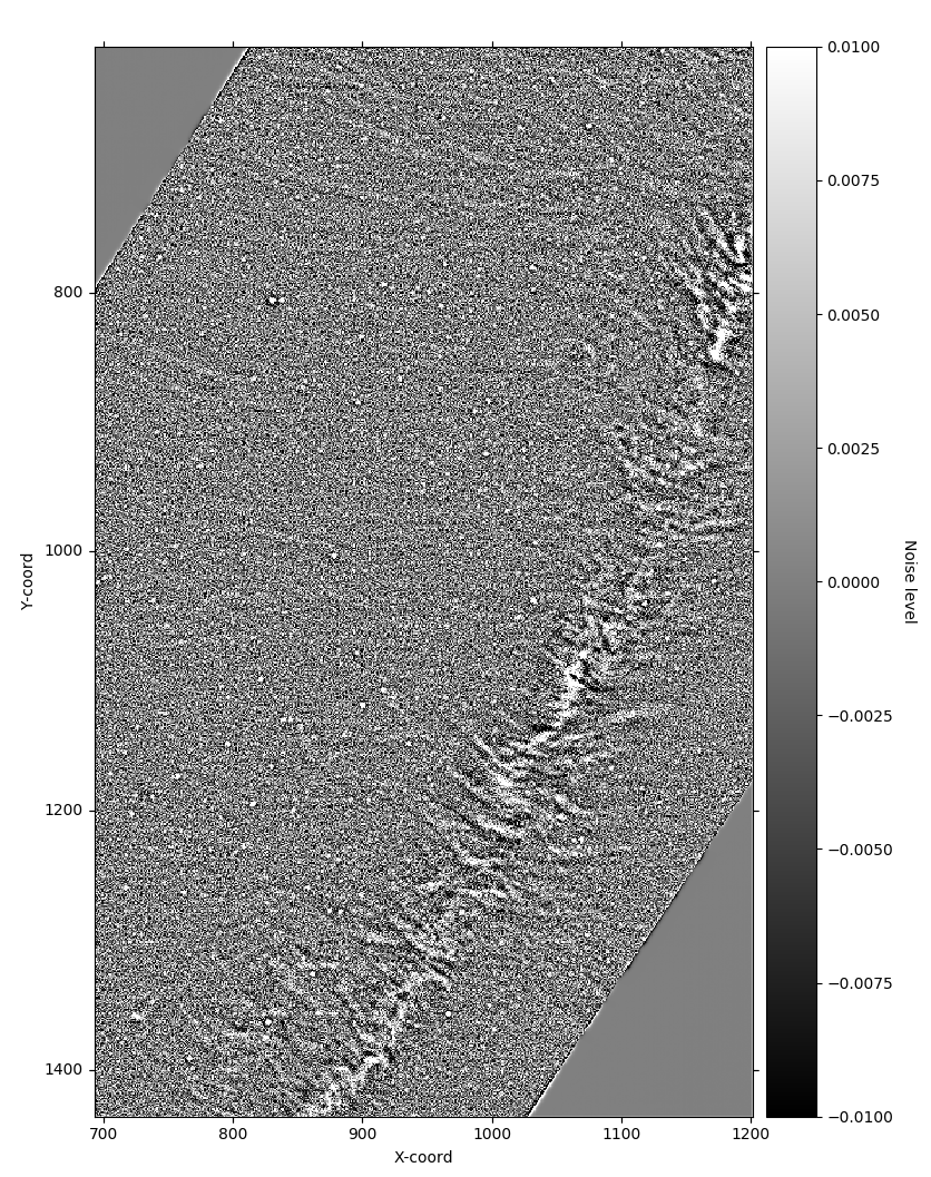
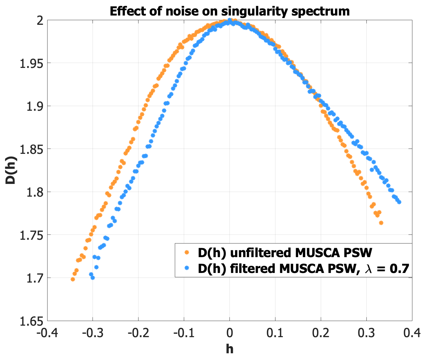
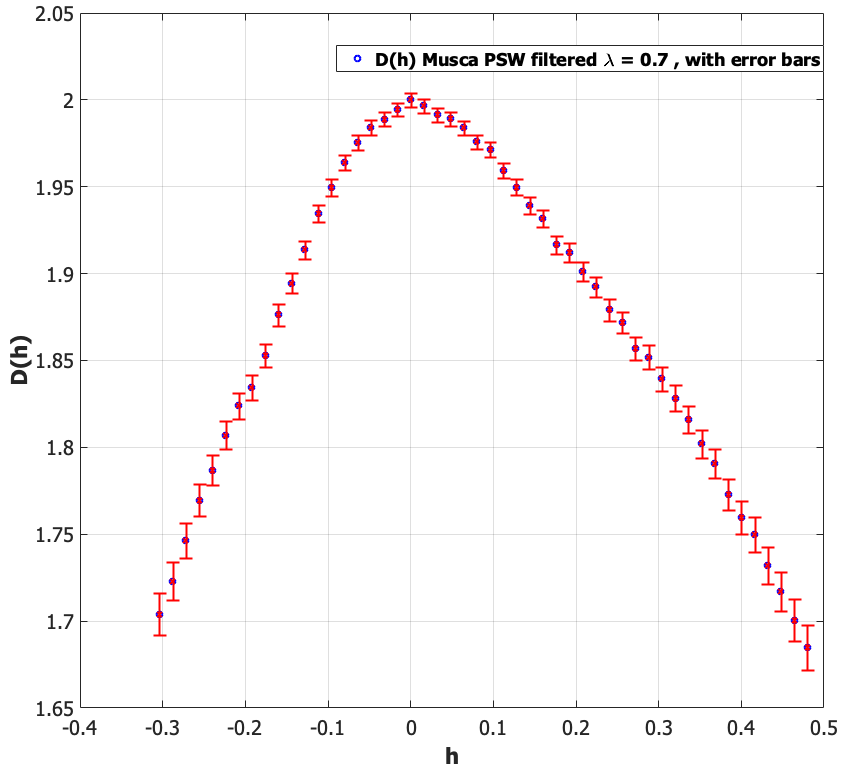
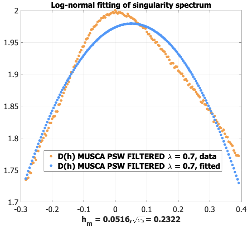
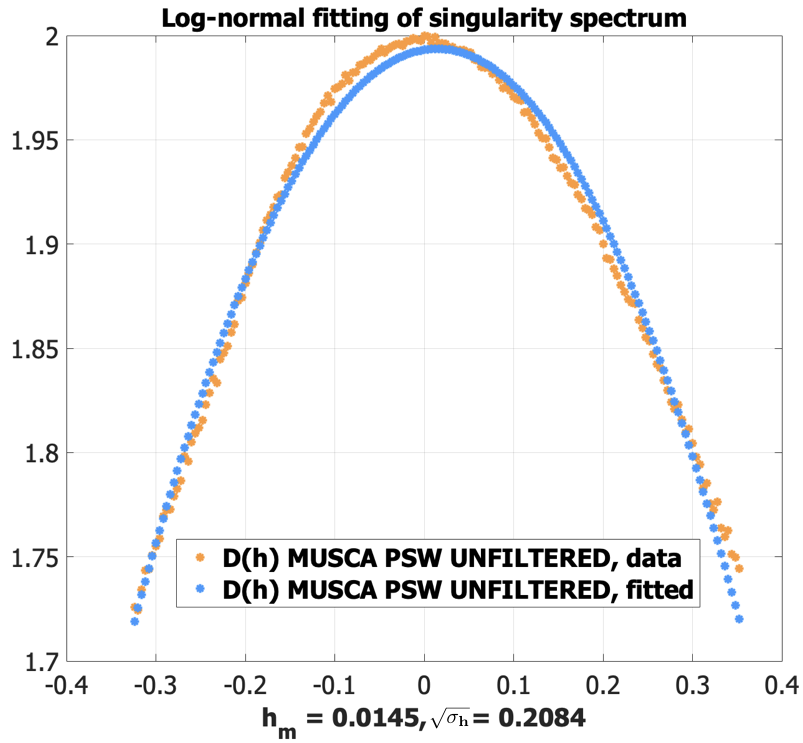
and $\lambda>0$ is a tuning parameter. The first term $\|s-s_{f}\|_{1}$ guarantees that the filtered image is very similar to the original (”data fitting term”), while the second term $\lambda\,\|\nabla s_{f}\|_{1}$, when minimized, promotes sparsity of the filtered gradients. Hence, the minimisation of the two terms eliminates noise, while keeping gradient information. To solve the minimization problem defined by eq. (22), we make use of the Half Quadratic Splitting resolution method (Geman & Chengda Yang 1995; Schmidt & Roth 2014). We show the result of sparse filtering first on the original flux density data in Fig. 8, where it appears as standard noise reduction. However, turning to the visualisation on the singularity exponents, as shown in Fig. 9, reveals the power of this sparse filtering with respect to the filamentary structures, as they are clearly enhanced with respect to the unfiltered version. We also observe that although the filtering does not eliminate much of background galaxies, it clearly eliminates sufficiently cosmic infrared background (CIB) and cosmic microwave background to significantly expose filamentary structures that were hidden by Gaussian noise in the original data. Figure 10 shows the image $s-s_{f}$, i.e., the resulting noise eliminated by the edge-aware filtering. Figure 11 displays the results of applying filtering for the singularity spectrum on the Musca map, with and without background noise elimination. Note how the background noise leads to an overestimation of the low dimensional filamentary structures, and how the gaussianity of background noise makes the nonfiltered spectrum more parabolic than the filtered one. Consequently, noise elimination is a necessary preprocessing step in a multifractal analysis of astronomical data for a better computation of the singularity spectrum.

Nevertheless, a question can be raised: does the edge-aware filtering defined by eq. (22) introduce spurious new gradients, initially not present in the original data? The answer is no, as can be seen from the numerical implementation of the minimization algorithm, which is performed in two steps:

1. Low level gradients are set to 0, and gradients whose norm is greater than a given threshold are kept. This operation does not introduce new gradients.

2. In a second step a new image is generated whose gradient is, at each point, a weighted sum of the original gradient image and the image obtained at the precedent step. This operation does not introduce new gradients either.

Figure 12: The mappings ${\bf h}\mapsto D({\bf h})$ computed for two consecutive scales of the unfiltered Musca 250 $\mu$m Herschel observational map using a reverse bi-orthogonal discrete wavelet transform of order 4.4. We see from the graphs that the presence of the noise alters the scaling of the measure.

Figure 13: Plot of $\zeta(q)$ for the Musca 250 $\mu$m Herschel observational map with filtering ($\lambda=0.7$, curve in red) and without filtering (curve in green); the mapping $q\mapsto\zeta(q)$ is defined by the structure function method (equation 25). We see on this graph that the background noise does affect the statistics of scaling.

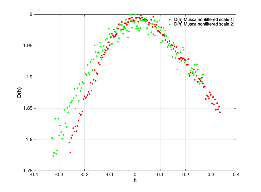
In Sects. 4 and Appendix B, we checked the scaling of the gradient measure by computening the singularity spectra at two consecutive scales in a wavelet projection of the signal. We observed from that experiment the scaling of the measure when the singularity spectra are derived from the computation of the singularity exponents using the method presented in Appendix B. These experiments were performed on the filtered Musca map with $\lambda=0.7$. We show in Fig. 12 the result of the same test using the nonfiltered Musca map. The two scaled versions are generated, like previously, using a reverse bi-orthogonal discrete wavelet transform of order 4.4. We see from the graphs that the presence of noise alters the scaling of the measure. This also advocates for the use of filtered observational maps.

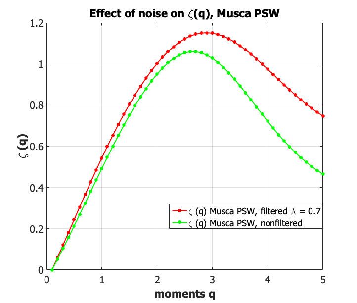
Figure 13 displays the result of the computation of the function $q\mapsto\zeta(q)$ defined in the structure function method (see Sect. 5.3, eq. 25) on the unfiltered and filtered Musca map. The two graphs are clearly distinct which adds to non negligible effects of the background noise on the scaling properties of the observational map.

Since the singularity spectrum is estimated from the histogram of the singularity exponents (see eq. 38), it is possible to estimate the error bars in the spectrum. If one discretizes the histogram of singularity exponents with a large number of bins, the probability $p_{\alpha}$ that a singularity exponent belongs to bin $B_{\alpha}$ can be estimated by $N_{\alpha}/N$, where $N$ is the total (large) number of realizations of the singularity exponents, and $N_{\alpha}$ is the number of samples falling in the bin indexed by $\alpha$. Then, if $N$ is large enough, $N_{\alpha}$ can be estimated by a Gaussian, and one can assign an error bar to the measurement by setting a 99% confidence interval. A computation using this hypothesis leads to the following values of the error bars (Turiel et al. 2006):

$$\Delta D({\bf h})=\displaystyle\frac{3}{\log{\bf r}_{1}}\cdot\frac{1}{\sqrt{N_{\bf h}}}$$ (24)

with $N_{\bf h}$ the number of events in the bin associated to singularity exponent ${\bf h}$, and ${\bf r}_{1}$ as the minimum resolution of the inertial range. Figure 14 displays the singularity spectrum with its error bars of the edge-aware filtered Musca 250 $\mu$m map with a parameter value $\lambda=0.7$.

Figure 14: Singularity spectrum of the Musca Herschel 250 $\mu$m map with error bars as defined by eq. 24; the observational map is edge-aware filtered with a tuning parameter $\lambda=0.7$.

5.3 Inertial range and the 2D structure function method

Figure 15: Result of the 2D structure function method for the determination of an inertial range of spatial scales. Computations are done on the Musca 250 $\mu$m map filtered data with $\lambda=0.7$ (eq. 22). $5\times 10^{8}$ couples of points $({\bf x}_{1},{\bf x}_{2})$ chosen uniformly in the spatial domain; moments $q$ are between 0.1 and 5 with increment step 0.1 (only some of the moments are shown for clarity). The left panel shows the graph of a $\log-\log$ plot (eq. 25) with colors indicating some moment values $q$. The image also shows the graphs of linear regression fits (dotted lines), performed in an inertial range covering the interval $[13,160]$ pixels, corresponding to the range of distance $[0.053,0.65]\leavevmode\nobreak\ \mbox{pc}$. The middle panel displays the resulting map $q\mapsto\zeta(q)$. The two panels on the right show the quality of linear regression: sse (sum of squares due to error), and the $r$ correlation coefficient. Hence the quality of the fit decreases with the moment order $q$.

Figure 16: Result of the 2D structure function method, applied over one of the MHD simulation outputs presented in Sect. 6, for the determination of an inertial range of spatial scales. $5\times 10^{8}$ couples of points $({\bf x}_{1},{\bf x}_{2})$ chosen uniformly in the spatial domain; the moments $q$ have values between 0.1 and 5 with increment step 0.1 (only few of the moments are shown for clarity). The first left panel shows the graphs of the $\log-\log$ plot (eq. 25, with colors indicating some moment values $q$). Like in Fig. 15, we also draw the graphs of linear regression fits (dotted lines) performed in an inertial range covering the interval of distance $[0.18,1.5]\leavevmode\nobreak\ \mbox{pc}$. The second panel displays the map $q\mapsto\zeta(q)$. The third and fourth panels show the quality of linear regression: sse (sum of squares due to error), and the $r$ correlation coefficient.

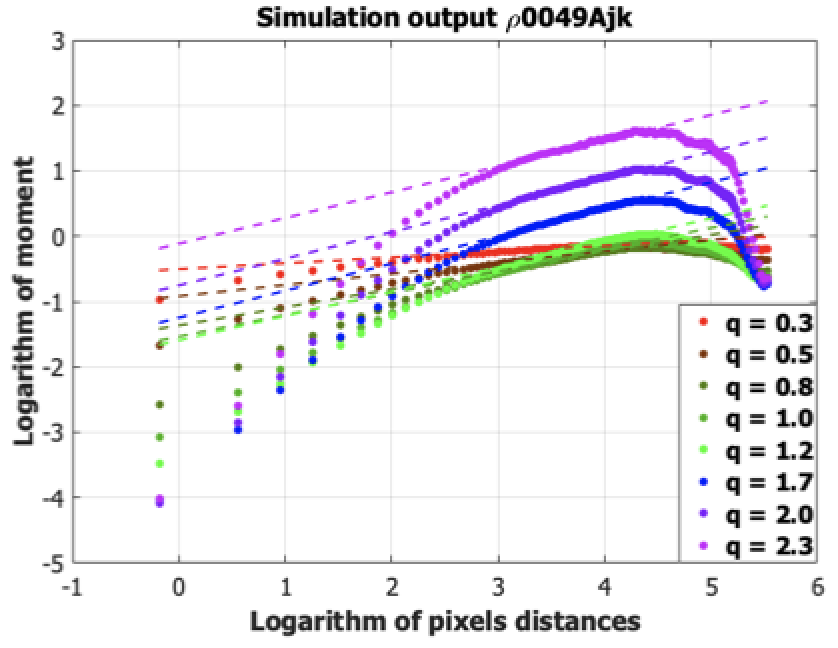
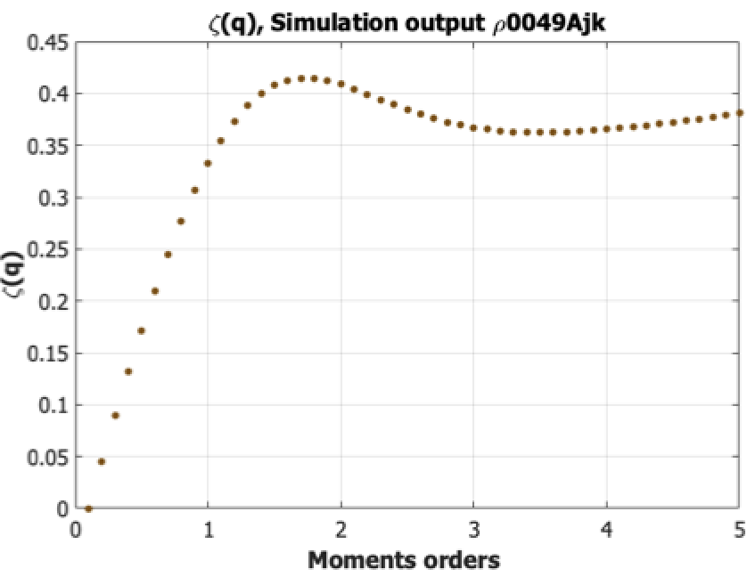
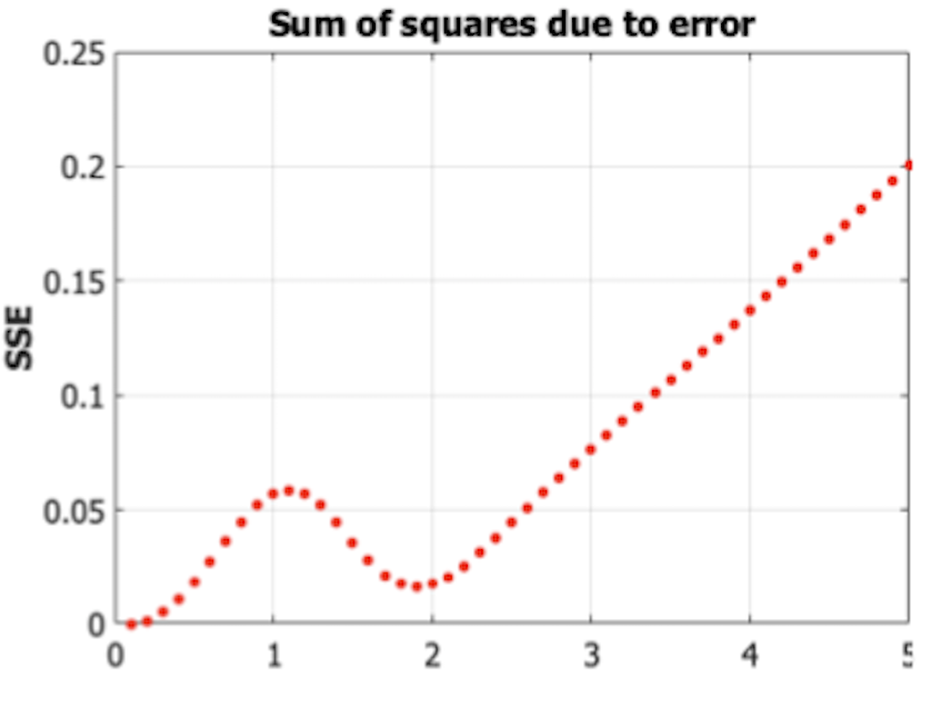
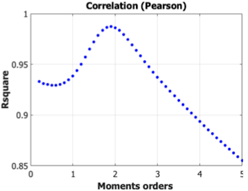
In a canonical approach to multifractality, the determination of scaling laws is achieved by statistical analysis of the moments of wavelets projections of the signal over a large range of scales, and a grand ensemble of realizations (Venugopal et al. 2006a). As mentioned before, verifying the existence of scaling laws through the computation on grand ensembles of realizations cannot be achieved with our single Musca image.

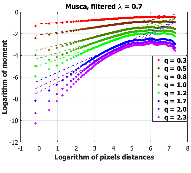
We thus have to use a spatial approach, based on 2D structure functions, introduced in Renosh et al. (2015) to check the existence of a significant inertial range. If ${\bf x}_{1}$ and ${\bf x}_{2}$ are points in the 2D signal domain, the existence of scaling laws for a certain range of spatial distances is verified when

$$\langle|s({\bf x}_{1})-s({\bf x}_{2})|^{q}\rangle\sim\|{\bf x}_{1}-{\bf x}_{2}\|^{\zeta(q)}.$$ (25)

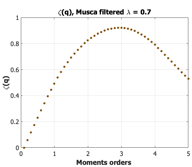
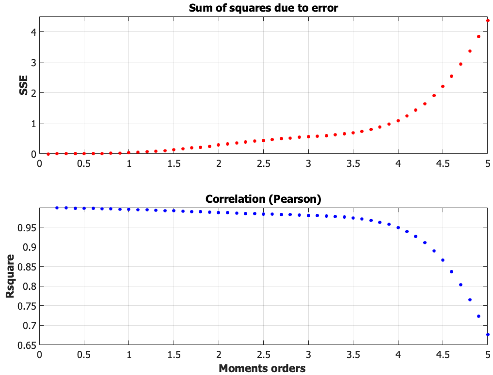
Consequently, the spatial moments $\langle|s({\bf x}_{1})-s({\bf x}_{2})|^{q}\rangle$ are $\log-\log$ plotted against the distances $\|{\bf x}_{1}-{\bf x}_{2}\|$ for a very large ensemble of couples $({\bf x}_{1},{\bf x}_{2})$. We carried out experiments on both original and edge-aware filtered data for $5\times 10^{8}$ couples of points $({\bf x}_{1},{\bf x}_{2})$, chosen randomly in the Musca map. We also conduct the experiment on MHD simulation outputs presented in Sect. 6. In Fig. 15 we show the result of the structure function method for the Musca 250 $\mu$m map filtered data with $\lambda=0.7$ (eq. 22). From left to right, the first image (top left) is the graph of a $\log-\log$ plot with colors indicating some moment values $q$. The image also shows the graphs of linear regression fits (dotted lines) performed in an inertial range covering the interval $[13,160]$ pixels, corresponding to the range of distance $[0.053,0.65]\leavevmode\nobreak\ \mbox{pc}$. Middle image displays the resulting map $q\mapsto\zeta(q)$. The two images on the right show the quality of linear regression, evaluated both with sse (sum of squares due to error), and the classical Pearson correlation coefficient $r$.

We note that the derived inertial range is probably affected by the beam size ($\sim$3 pixels, 0.012 pc) for the lower boundary (0.05 pc), and by the sizes of the rectangular map (1786 pixels in the $x$ direction i.e. 7.144 pc, 2135 pixels in the $y$ direction i.e. 8.54 pc) for the upper boundary (0.65 pc).

6 MHD simulation data

The simulations used in this work are presented in (Dib et al. 2007, 2008). Here, we recall their basic features. The ideal MHD equations are solved on a uniform 3D cubic grid using a total variation diminishing scheme (TVD), which is a second-order-accurate upwind scheme (Kim et al. 1999). The boundary conditions used in the three directions are periodic. The Poisson equation is solved to account for the self-gravity of the gas using a standard Fourier algorithm. In order to achieve second-order accuracy in time, an updated step of the momentum density due to the gravitational force is implemented, as in (Truelove et al. 1998).

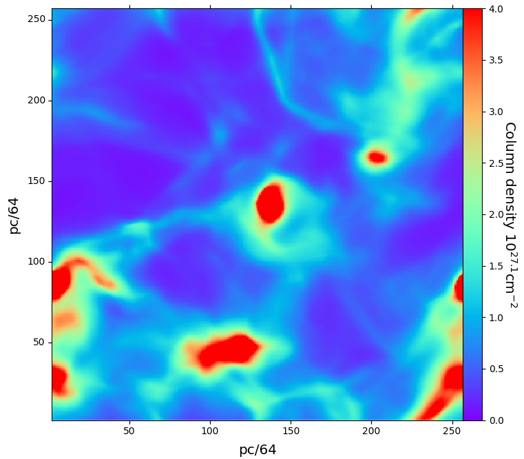
Following the method described in (Stone et al. 1998), turbulence is continuously driven in the simulation box and the kinetic energy input rate is adjusted such as to maintain a constant specified ${\it rms}$ sonic Mach number $M_{s}=10$. Kinetic energy is injected at large scales, in the wave number range $k=1-2$. When converted into physical units, the models correspond to a box size of 4 pc and an average number density of $500$ cm^-3. The corresponding column density is thus $\sim 5\,10^{21}$ cm^-2, which is similar to that of many molecular clouds except for those associated with massive star formation. The temperature is 11.4 K, the sound speed $0.2$ km s^-1, and the initial rms velocity is 2 km s^-1 (i.e., therefore the initial sonic Mach number is $M_{s}=10$). The four simulations vary by the strength of the initial magnetic field ranging from a magnetically subcritical cloud model to a non-magnetic cloud. The strength of the initial magnetic field in the box for the subcritical, moderately supercritical, and strongly supercritical magnetized models are $B_{0}=45.8,14.5$, and $4.6$ $\mu$G, respectively. This corresponds to $\beta$ plasma and mass-to-magnetic flux values of the box for these runs of, $\beta=0.01,0.1$ and $1$, and $\mu_{box}=0.9,2.8$, and $8.8$, respectively. The simulations start with a uniform density field, and are evolved for half a sound crossing time (the sound crossing time is $t_{s}=20$ Myrs), equivalent to 5 turbulent crossing times (the turbulent crossing time is $t_{c}=2$ Myrs), before self-gravity is turned on. This is a common practice in such simulations and a necessary step in order to allow for the full development of the turbulent cascade. Left image of Fig. 17 displays the integrated column density maps of one snapshot corresponding to the hydrodynamical case with no magnetic field at a time $t=0.422\,t_{c}$ Myrs after gravity is turned on.

In Fig.  16 we show the result of the determination of inertial range with the 2D structure function method (Sect. 5.3) applied over one MHD simulation output. We see considerable differences compared to the Musca 250 $\mu$m observational map results, notably in terms of quality of the linear regression. The range of distances chosen for performing the linear regression fit is $[0.18,1.5]\leavevmode\nobreak\ \mbox{pc}$. Other outputs in the MHD simulation show similar plots. Hence, the scaling properties of MHD simulation outputs are different compared to real observation maps.

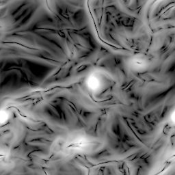
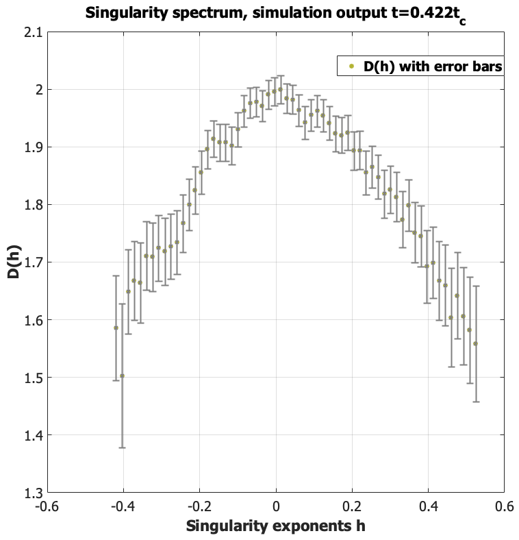
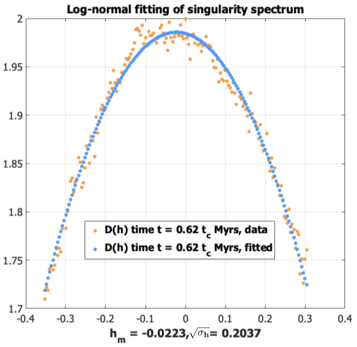
In the middle and right panels of Fig. 17 we also show the singularity exponents and the singularity spectrum as described in Sect. 3.3 . Note that the error bars display more uncertainty than those of the Musca 250 $\mu$m map displayed in Fig. 14: this larger uncertainty arises from the low number of samples (the image data is of size ($256\times 256$). In Fig. 18, we display both the singularity spectrum (curve in orange) and the computation of a fitted $\log$-normal spectrum (in blue) $D({\bf h})=\displaystyle 2-\frac{1}{2}\left(\frac{{\bf h}-{\bf h}_{m}}{\sigma_{{\bf h}}}\right)^{2}$ (eq. 9) for the data corresponding to time $t=0.62\,t_{c}$ Myrs after gravity is turned on. The fitting is performed using the Quasi-Newton minimization algorithm implementation available in Matlab. We get here ${\bf h}_{m}=-0.0223$, $\sigma_{{\bf h}}=0.2037$. Hence, in this case $D({\bf h})=2-\displaystyle\frac{({\bf h}+0.0223)^{2}}{0.0829}$. The fit is very good, which indicates a good approximation by a $\log$-normal process. This good fit was observed for all our simulation outputs. In comparison, looking at Figs. 14 and 19 we conclude that the singularity spectrum of the Musca 250 $\mu$m map does not fit so well with a $\log$-normal process. We will discuss this point in the next sections.

Figure 17: Left panel: one snapshot of column density output of the MHD simulation data used in this work, integrated along one axis of the cube. The output shown here corresponds to the hydrodynamical case with no magnetic field at time $t=0.422\,t_{c}$. Middle panel: map of the singularity exponents. Right panel: singularity spectrum with its error bars computed using eq. (24).

Figure 18: Log-normal fit of the singularity spectrum for the data corresponding to time $t=0.62t_{c}$ Myrs after gravity is turned on. In orange, the singularity spectrum computed in the microcanonical framework. In blue, a fitted quadratic $\log$-normal singularity spectrum. The fit is very good, which indicates a good approximation by a $\log$-normal process.

Figure 19: These two figures show the results of a $\log$-normal fit for the singularity spectrum of the full Musca 250 $\mu$m map (also called ’PSW’), edge-aware filtered (top image, $\lambda=0.7$) and unfiltered (bottom image). In each image, the singularity spectrum ${\bf h}\mapsto D({\bf h})$ is shown in orange, and the $\log$-normal parabola in blue. The values obtained for the coefficients of the fit (equation 9) are given in each case. The differences in the two fits underline the importance of the edge-aware filtering for multifractal analysis of astronomical observational maps. It appears that the background noise ”$\log$-normalizes” the data, while the filtered version, which better takes into account fine filamentary structures, deviates from $\log$-normality. Note in particular, in the filtered version, the change in the orange curve around ${\bf h}=-0.2$. This is an indication that different types of turbulent processes are present in the Musca cloud, in particular those processes inside the main filament and the surrounding cloud.

7 Multifractal analysis of data

7.1 Detection of a multiplicative cascade

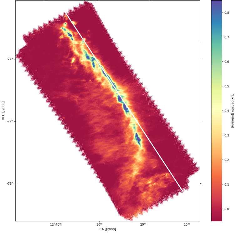
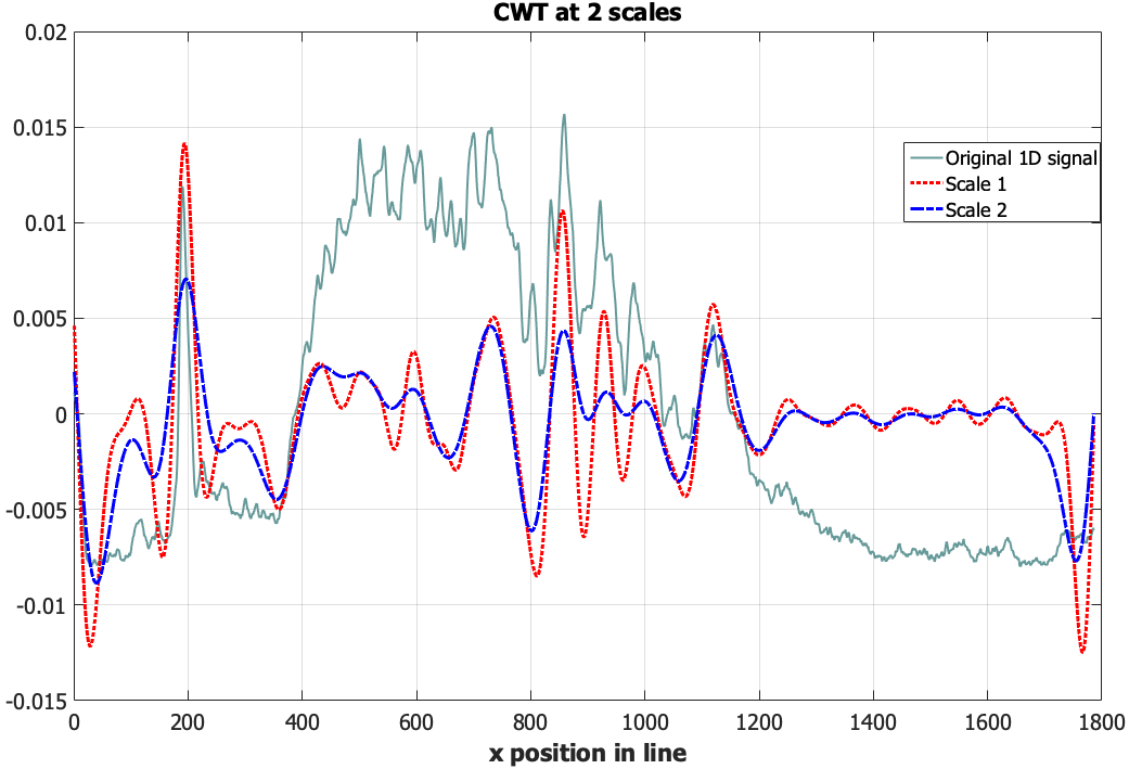
To investigate the existence of a multiplicative cascade in the Musca map, we use the cumulant approach described in Appendix C. The cumulant analysis is performed over 1D signals which are extracted from columns of a 2D observational map as shown in the left panel of Fig. 20. In this figure we display, as an example, a 1D signal that comes from a particular column in the Musca observation map; that column crosses low and high flux regimes, i.e. regions outside and inside the main filament. We perform the cumulant analysis using the mexican hat as analyzing wavelet:

$$\psi({\bf x})=\displaystyle\frac{2}{\pi^{1/4}\sqrt{3\sigma}}\left(\frac{{\bf x^{2}}}{\sigma^{2}}-1\right)e^{\frac{-{\bf x}^{2}}{2\sigma^{2}}}$$ (26)

(second derivative of a gaussian) with a deviation $\sigma=3.2$ chosen for the data. If $f({\bf x})$ is a 1D signal, the continuous wavelet projection (CWT) of $f$ at scale ${\bf r}>0$ is

$${\cal T}_{\psi}(f)({\bf x},{\bf r})=\displaystyle\frac{1}{{\bf r}}\int_{\mathbb{R}}f({\bf u})\psi\left(\displaystyle\frac{{\bf x}-{\bf u}}{{\bf r}}\right)\,\mbox{d}{\bf u}.$$ (27)

Note that we use $L^{1}$ normalisation instead of $L^{2}$: to study correlations, the conservation of energy is not necessary, while $L^{1}$ normalisation better adapts to strong variations in the signal (Venugopal et al. 2006a). We use the Herschel 250 $\mu$m Musca dataset filtered with $\lambda=0.7$ (eq. 22 in Sect. 5.2). Figure 20 shows a selected column in the Musca map and the associated 1D signal $f({\bf x})$ with two of its wavelet projections ${\cal T}_{\psi}(f)({\bf x},{\bf r})$ at two respective scales ${\bf r}_{1}$ and ${\bf r}_{2}$ with ${\bf r}_{2}<{\bf r}_{1}$ (graphs in red and blue respectively).

Figure 20: Left panel: Musca 250 $\mu$m map in which the white column defines a 1D signal. Right panel: original 1D signal (centered and rescaled) and CWT projections of the selected 1D signal with the Mexican hat wavelet respectively at scales 5 (red) and 60 (blue).

Figure 21: Plots of the $\log$-correlations ${\cal C}({\bf r},\Delta{\bf x})$ vs $\log(\Delta{\bf x})$ for two 1D signals extracted from the Musca 250 $\mu$m map according to the scheme shown in Fig. 20. The analyzing wavelet is given by equation 27 with $\sigma=3.2$. We use 500 scales from ${\bf r}=1$ to ${\bf r}=500$ and 400 values for $\Delta x$ between 1 and 400. The chosen values for the scales are enough to highlight more than 2 nodes in a cascade, if such a cascade exists. Each image shows the graphs of the log-correlations for few scales (curves from green to purple corresponding to increasing scales), and the line $y=-c_{2}\log(\Delta x)$ with the slope $c_{2}$ computed through linear regression, according to eq. 48. The linear regression used to compute $c_{2}$ is performed for scales between 10 and 200. The left panel shows the $\log$-correlations corresponding to column 970 in the Musca observational map. We see that the graphs of ${\cal C}({\bf r},\Delta{\bf x})$ for different scales follow the slope given by the line $y=-c_{2}\log(\Delta x)$. The right panel, corresponding to column 947, displays a different behavior: we observe long-range correlations, but the behavior seen in a multiplicative cascade is not present.

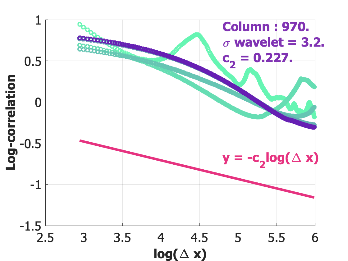
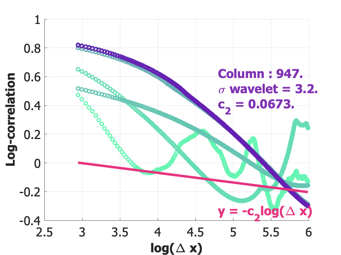
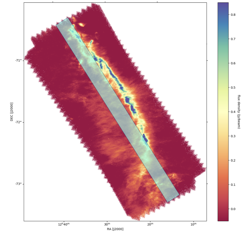
We apply this cumulant analysis on each 1D signal (columns) by computing the $\log$-correlations ${\cal C}({\bf r},\Delta{\bf x})$ (eq. 50) and plot them against $\log(\Delta{\bf x})$. As explained in Appendix C, we look for fingerprints of long-range correlations and the existence of a multiplicative cascade according to ${\cal C}({\bf r},\Delta{\bf x})\sim\log\Delta{\bf x}$ and eq. 51. We use 500 scales from ${\bf r}=1$ to ${\bf r}=500$ and 400 values for $\Delta x$ between 1 and 400. The slope $c_{2}$ is computed through linear regression, according to eq. 48. The linear regression used to compute $c_{2}$ is performed for scales between 10 and 200. Our experiment shows that long-range correlations are found for all 1D columns, and that a multiplicative cascade does exist in the Musca cloud. The left panel in Fig. 21 displays an example, corresponding to column 970 in the Musca map, of a typical graph obtained in Musca: the $\log$-correlations corresponding to different scales decrease in accordance with the equation of the line $y=-c_{2}\log(\Delta x)$ for the computed $c_{2}$ value, which is an indication for the presence of a multiplicative cascade in the column. However, there exists an interval of columns, corresponding to the rectangular area shown in Fig. 22 (left), for which the curves behave as shown in the right panel of Fig. 21. This does not imply the absence of a multiplicative cascade, but there is an area, inside this region, which brings perturbations to the statistics; this is also an indication that different processes are at work inside the Musca cloud.

Figure 22: Left: in the rectangular area shown in the picture, the statistics of the $\log$-correlations are different than in other parts of Musca). Right: definition of 6 ROIs (regions of interest) inside Musca ISM.

Figure 23: Left: the singularity spectrum of the filtered ($\lambda=0.7$) Musca 250 $\mu$m observational map (in orange) is fitted against a $\log$-normal parabolic spectrum (blue) defined by equation (9). The fit is performed using the Quasi-Newton minimization algorithm implementation available in Matlab. Right: the singularity spectrum of the of the filtered ($\lambda=0.7$) Musca 250 $\mu$m observational map (in orange) is fitted against a $\log$-Poisson singularity spectrum (blue) defined by equation (10). Same minimization algorithm. Both images display the values found by minimization algorithm and the error fit.

Figure 24: The images display, for each region of interest in the Musca cloud delimited in Fig. 22: the singularity spectrum ${\bf h}\mapsto D({\bf h})$ of a ROI in orange color, a $\log$-normal fitted approximation singularity spectrum in blue (equation 9), the obtained numerical values ${\bf h}_{m}$ and $\sigma_{{\bf h}}$, the error of the fit. The various values of ${\bf h}_{m}$ and $\sigma_{{\bf h}}$ for each ROI are also given in table 1

7.2 Musca spectrum: multifractality, $\log$-normality

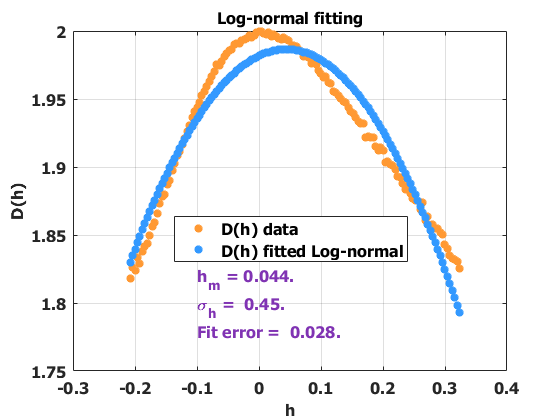
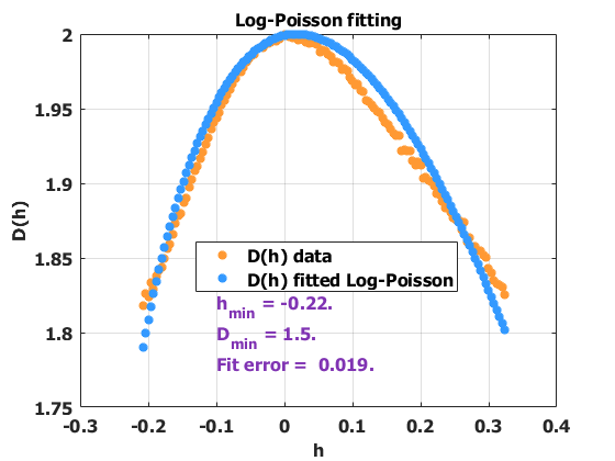
Our final singularity spectrum obtained for the whole Musca region is displayed in Fig. 14. In contrast to previously obtained singularity spectra for the ISM (e.g. Khalil et al. (2006); Elia et al. (2018)), this improved spectrum appears not very symmetrical with a clearly steep, almost linear, descend in the ${\bf h}\leq 0$ side (left) and a more round, gaussian like shape for the ${\bf h}\geq 0$ side (right). We note that this clear asymmetric shape has been enhanced and well revealed thanks to the noise filtering (see Fig. 11). Despite this clear asymmetry, we fitted in Figure 23-left the obtained spectrum with a parabolic curve which would represent a log-normal behavior of the turbulent fluctuations. We find, ${\bf h}_{m}=0.0206$, $\sigma_{{\bf h}}=0.4564$. The part of the singularity spectrum corresponding to ${\bf h}\leq 0$ shows a clear deviation between the spectrum computed in the microcanonical formalism (orange) and the parabolic (blue), which seems to strongly point to some non $\log$-normal process in the turbulent flow of Musca. We note that there is actually more resemblance with a $\log$-Poisson spectrum as shown by the fit displayed in Fig. 23-right. A $\log$-Poisson spectrum is indeed asymmetric with a steep descend in the negative ${\bf h}$ side (see Fig. 2). These fit results can be compared with the bottom panel of Fig. 19, which corresponds to the non-filtered case. Given that the noise filtering enhances mostly the contrast of filamentary structures (which were otherwise merged in the noise data), it suggests that the asymmetry in the singularity spectrum and the $\log$-Poisson behavior are related to 1D structures, i.e. filaments as expected for the most singular structures in a turbulent cascade with intermittency (see (She et al. 1990) and Sect. 3.1 below for a discussion). In the next section, we will see that some regions of Musca are ”more $\log$-normal” than others.

Furthermore, in addition to the possible proxy of the whole spectrum by a $\log$-Poisson curve, by a close inspection of Fig. 14, we note around ${\bf h}=-0.2$ a slight non-convex area in the graph. This observation can be made only on the edge-aware filtered signal, because the background noise ”smoothes” the spectrum as seen in the orange graph of Fig. 11. Consequently, the singularity spectrum in this case seems to present two local extrema. This might be an indication that at least two different processes can be present in the signal.

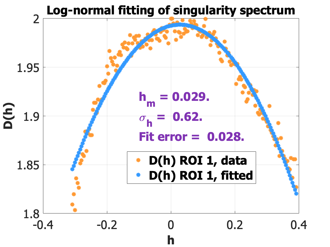
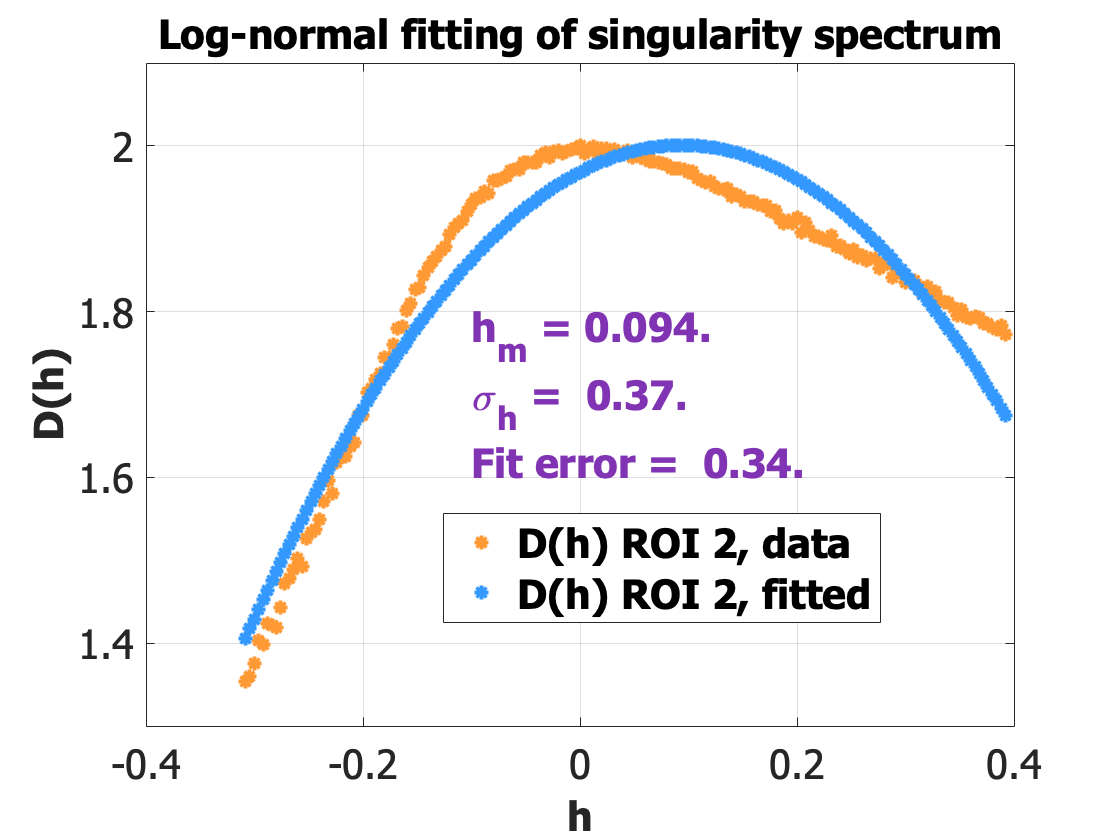
ROI	${\bf h}_{m}$	$\sigma_{{\bf h}}$	Error	$[{\bf h}_{1},{\bf h}_{2}]$	Std dev.
ROI1	0.029	0.62	0.028	$[-0.3,0.4]$	0.057
ROI2	0.094	0.37	0.34	$[-0.3,0.4]$	0.16
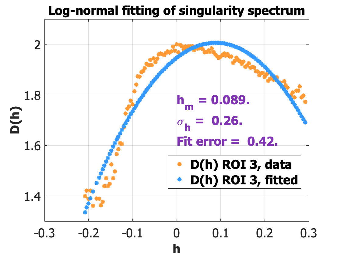
ROI3	0.089	0.26	0.42	$[-0.2,0.3]$	0.18
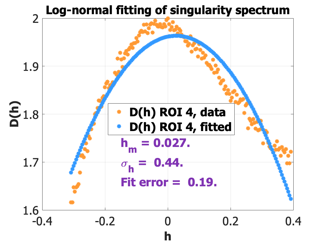
ROI4	0.027	0.44	0.19	$[-0.3,0.4]$	0.1
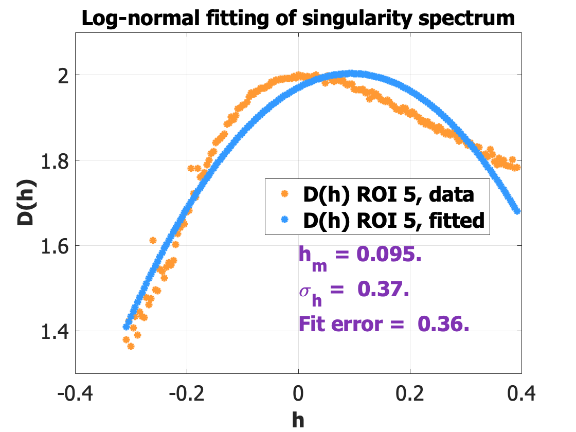
ROI5	0.095	0.37	0.36	$[-0.3,0.4]$	0.16
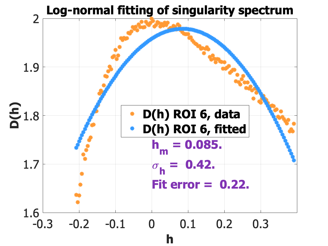
ROI6	0.085	0.42	0.22	$[-0.2,0.4]$	0.087

Table 1: Parameters of fitted $\log$-normal process for each ROI: column 1: ROI, column 2: ${\bf h}_{m}=\langle{\bf h}\rangle$ average of singular values, column 3: $\sigma_{{\bf h}}$ singularity dispersion (see equation 9), column 4: fit error = $\|D({\bf h})-D_{\mbox{logn-fit}}({\bf h})\|_{2}^{2}$, column 5: interval $[{\bf h}_{1},{\bf h}_{2}]$ chosen according to error bars of singular values in which the statistics ${\bf h}_{m}$, $\sigma_{{\bf h}}$, the standard deviation and the fit error are computed, column 6: standard deviation of each ROI singularity spectrum within the specified interval of ${\bf h}$ values shown in column 5.

7.3 Distinct statistical properties observed in the data

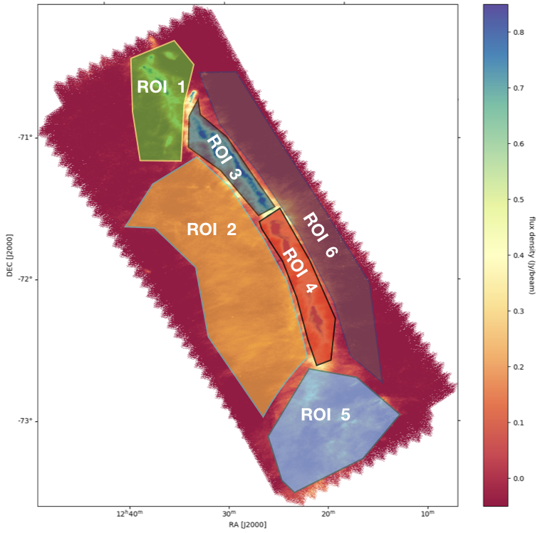
To go one step further, we now compare singularity spectra computed over different regions of interest (ROI) to reveal potential different turbulent behaviors inside the cloud. Figure 22 shows the geometric location of 6 ROIs inside the Musca cloud that were selected based on different physical properties. ROI1 is the northern end of the filament where a single protostellar object is located. ROI2 represents the eastern cloud area with prominent striations (weak filamentary structures perpendicular to the main crest of Musca filament). ROI3 and ROI4 are the highest density crest regions. We define two ROIs on the crest with ROI4 being the southern part with already signs of fragmentation while in ROI3 the northern part, the crest is still very much homogeneous. ROI5 is the southern end of the filament which is less organized in filaments or striations. ROI6 is the western part of the embedding cloud with less prominent striations. For each ROI, we compute: the singularity spectrum and the values ${\bf h}_{m}$ and $\sigma_{{\bf h}}$ of a fitted $\log$-normal spectrum $D_{\mbox{logn-fit}}({\bf h})=\displaystyle 2-\frac{1}{2}\left(\frac{{\bf h}-{\bf h}_{m}}{\sigma_{{\bf h}}}\right)^{2}$. The quality of the fit is estimated by the $L^{2}$ error $\|D({\bf h})-D_{\mbox{logn-fit}}({\bf h})\|_{2}^{2}$. The best defined curves are the ones with the highest number of pixels, i.e. ROI2 and ROI5. Figure 24 and Table 1 show the results of the computations. The obtained graphs and values confirm that the processes inside each ROI can display strong deviation from a $\log$-normal process. First, it becomes obvious that we can distinguish two classes of curves, the ones that are not too far from a $\log$-normal fit, ROI1 and - to a lesser extent - ROI4 (with respective fit errors 0.028 and 0.19), and the remaining ones that deviate significantly from $\log$-normality. ROI1 and ROI4 have the largest singularity dispersions $\sigma_{{\bf h}}$ of a fitted $\log$-normal with $\sigma_{{\bf h}}$ = 0.62 and 0.44, respectively. Moreover, ROI1 and ROI4 feature the most symmetric singularity spectra among the ROIs. The other ROI’s all show a steeper slope at negative h values than at positive ones and ROI2 features the worst $\log$-normal fit among the 6 ROIs; this result that can be put in relation with, for one part, the large density of striations seen in ROI2, and for another part with Fig. 22 and the discussion in Sect. 7.1: it is likely that the part of rectangle shown in Fig. 22 that intersects ROI2 is responsible for deviation also observed in the $\log$-correlations ${\cal C}({\bf r},\Delta{\bf x})$. For all ROI’s except of ROI1 and ROI4, the singularity spectrum is more of the $\log$-Poisson type than $\log$-normal. This finding also applies to the singularity spectrum of the whole (edge-aware filtered) Musca observational map as can be seen in Figs. 14, 19, and 23.

7.4 Application on data from simulations

Figure 25: Variation in time of the fitted $\sigma_{\bf h}$ of $\log$-normal singularity spectrum (equation 9) for the simulation outputs described in Sect. 6. Value of the magnetic pressure $\beta=0.1$,

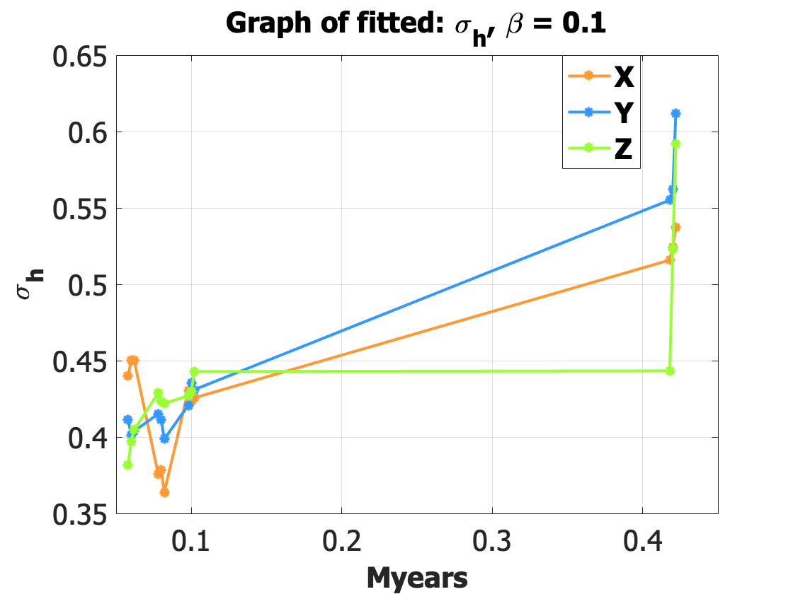
Figure 18 shows a typical result of a $\log$-normal fit applied on one projection of the MHD simulation data presented in Sect. 6 (by projection we mean here in one of the three spatial directions -X, Y or Z- since the data is in the form of a 3D cubic volume): the fit is very good, in all directions, and this is true for all available simulation outputs. Consequently, we can say that the MHD simulation outputs are $\log$-normal processes, and it is then possible to see the variation in time of the width of the $\log$-normal fitted singularity spectrum (the coefficient $\sigma_{\bf h}$ of eq. 9). Figure 25 displays the graph of the dispersion of the fitted $\log$-normal process, or $\sigma_{\bf h}$ of eq. 9 as a function of time, in MYr, for the value $\beta=0.1$. The dispersion becomes wider as gravitational effects become much more pronounced (more bound and collapsing structures), as was already stated in Elia et al. (2018), where the authors note that when gravity is present one gets a broader spectrum, and this is also the case when turbulence is driven with compressive modes. Compressive driving generates larger density contrasts in the simulations volume and in the resulting 2D maps. This effect mimics the presence of gravity. Accordingly, in the $\log$-normal approximation, the dispersion $\sigma_{\bf h}$ can be used as an indication of the gravitational effects.

8 Discussion of results: Musca turbulent dynamics and implication on star formation processes

Figure 26: Distribution of the singularity exponents in ROI1 (left) and in the southern region of Musca ROI5 (right). Both regions show complex linear structures, but of different sizes and organisation.

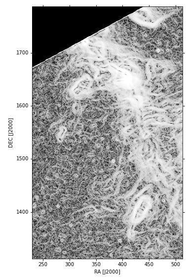
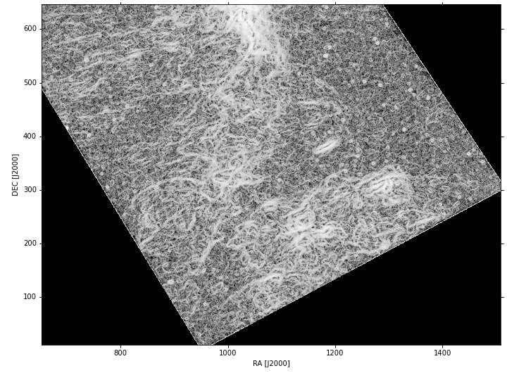
As discussed for instance in Bonne et al. (2020a), several physical processes are presumably at work to explain the formation of the Musca filament in particular, as well as the global behavior of the ISM in this molecular cloud. We have to consider the turbulence injected from large scales, self-gravity presumably acting at small scales, magnetic field pressures and tensions at all scales, and possibly some local effects such as shocks. Our long term goal is to seek for statistical signatures of these different processes thanks to the multifractal analysis, introduced in this paper, and profiting from the unprecedented depth and richness of Herschel maps. Facing the numerous difficulties in deriving such clean statistical probes, in investigating the possible different signature of processes and the inherently complex situations of the real data, the present article should be seen as a first step towards this long term ambitious goal. The following discussion thus only provides hints for new directions which will need confirmation and further interpretations thanks to extensive studies on simulations and on a large number of star-forming regions.

The fact that we clearly found a multiplicative cascade with a significant and large inertial range from at least 0.05 to 0.65 pc is an important step to support the turbulence interpretation of the dust emission from Herschel towards a weak column density cloud surrounding the low-mass Musca filament. This result points to a dominance of turbulent motions, and confirms that this turbulent behavior originates from at least pc scales.

With the help of this new microcanonical approach which does not require multiple realizations (single map), we could then derive for the first time a precise enough singularity spectrum of the observed flow to characterize its turbulent behavior. We verified that we have a good invariance of the singularity spectrum to the scale which was not obtained with box counting method for instance. This is highly important as we believe this is the missing step to be able to derive the true, relatively precise singularity spectra of our datasets (real data and simulations) and to quantify some differences between regions and between observations and simulations to progress on the understanding of the physics leading to cloud and filament formation.

The obtained singularity spectrum confirms that the ISM towards Musca and its surroundings has a clear multifractal structure. It implies the existence of intermittency and non-gaussian behavior which are believed to be critical to explain the formation of the densest and star forming structures. Moreover, while the so far derived singularity spectra were often found to have a $\log$–normal behavior in previous works, we here clearly obtain a global singularity spectrum which strongly deviates from $\log$-normality. Deviation from $\log$-normality here is apparent as the singularity spectra are clearly non-symmetric. Among the many multifractal processes having a non-symmetric spectrum, we discussed here the simplest case which is the $\log$-Poisson behavior which has been extensively discussed in the literature on turbulence. According to Gledzer et al. (1996) for instance a $\log$-Poisson behavior is expected for an energy cascading model of intermittency involving rare localized regions of both large and/or weak energy dissipation (dynamical intermittency) while a $\log$-normal behavior is obtained for intermittency arising from widespread regions with nearly equal dissipation rates (space intermittency). The existence of such geometric models for the $\log$-Poisson spectrum is interesting in astronomy, although further analysis must be done in order to relate the observed statistics with a particular type of process. Indeed, in all the ROIs chosen in the Musca map, and even in the ROI1, we can see filamentary and linear structures of various sizes and orientations on the map of singularity exponents, Consequently, it could be the distribution of these structures which affects the $\log$-normality of a singularity spectrum. See Fig. 26. Interestingly enough according to She et al. (1990) the most intermittent structures in incompressible purely hydrodynamical turbulence have to be filamentary to be stable. In the case of compressible and magnetised turbulence, we can only expect that these filaments are more stable.

We therefore propose that the ISM associated with the Musca filament region shows a turbulent behavior which is better reproduced by a dynamical intermittency than by a space intermittency with localized enhanced dissipation locations. From the global view discussed for instance in Bonne et al. (2020a) and from the realistic view that most intermittent regions have to be filamentary (She et al. 1990; She & Leveque 1994) we could then speculate that these localized enhanced dissipations are associated with the formation of the Musca filament and with the striations in the surroundings, and could be related to the efficient guiding and focusing by the magnetic field (reducing the space dissipation) towards a region of strong accumulation of matter where dissipation could be enhanced in accretion events. Local (accretion) shocks, providing strong local turbulence dissipation may explain and complement our understanding of the particular statistics ($\log$-Poisson type) of the large singularities of the map (large ${\bf h}$ values, i.e. the locations of large local gradients as imaged in white in the singularity map of Fig. 7). The fact that we find the most non-symmetric (hence, possibly $\log$-Poisson) singularity spectra towards the ROIs associated with the filaments of Musca reinforces this interpretation that the dynamical intermittency is associated with filament formation.

Interestingly enough, using the same microcanonical analysis we could not identify in simulated data a similar $\log$-Poisson behavior. From simulated datasets we always obtain $\log$-normal spectra. This behavior could perhaps reflect the fact that these simulations are run with a continuous injection of well behaved turbulence at large scales. The fact that self gravity is included does not seem to affect the singularity spectra. We clearly need to continue to investigate what is missing in the simulations to properly reproduce the observed data, but we can note that we have found a statistical tool sensitive enough to make the difference between simulations and real datasets.

9 Conclusion

In this work we make use of a new computable multifractal formalism in a microcanonical formulation, based on ideas from predictability in complex systems, and we apply it to analyze the complex turbulent structure of the ISM for the case of a Musca Herschel observational map. We confirm that to be fully effective, the use of the multifractal formalism must be operated with important checks on an observational map: determination of the inertial range for which scaling laws apply, scale invariance must be checked by computing singularity spectra at different scales and checking their coincidence, background noise elimination must be operated with particular care in order to preserve low dimensional weak coherent structures.

Our aim is to present a self-contained study with sufficient detail to help reproduce the experiments. Very importantly, we could make the check of scaling laws and the determination of the inertial range, such as usually done in canonical formulations, thanks to moments of the chosen partition functions achieved using a 2D structure function methodology. The microcanonical formulation is based on the direct computation of the singularity exponents. The singularity spectra are derived, and we check the invariance of the resulting spectra with respect to scale. Background noise has the tendency to $\log$-normalize the signals, by making their spectra parabolic. We propose a $L^{1}$ denoising algorithm based on edge-aware filtering which preserves low-dimensional features as opposed to thresholding through wavelet decomposition methods. We use the theory of cumulants to determine the presence of a multiplicative cascade using $\log$-correlations.

The results show a clear multiplicative cascade with a significant and large inertial range from at least 0.05 to 0.65 pc (larger scales might be affected by the $\sim 4\,$ pc width of the observed map, and smaller scale by the 0.012 pc beam size) pointing to a dominance of the turbulence originating from scales probably larger than a parsec. We show that a precise study of the intermittency can be achieved by the methodology introduced in this work. For the time in ISM studies, our data and analysis challenge the $\log$-normality of the singularity spectrum of the turbulence. This is one of the major results of this work. It suggests that the turbulence associated with the Musca filament formation exhibits more a dynamical intermittency with localized, enhanced energy dissipation than a space intermittency. Some hints for different turbulent behavior in the region and for some missing physics in simulations shows that the work presented in this study is only a first step in our long term goal to seek for statistical signatures of different turbulent, physical processes at work in the ISM.

Appendix A Definition of the measure

We keep the notations and conventions defined in Sect. 3.3. Let us begin by considering the set ${\cal V}_{n}({\bf x})$ displayed on the left of Fig. 4. In that case each ${\cal V}_{n}({\bf x})$ is made of two points and we introduce the discrete measure noted $\mu_{n}$ on the unit square by

$$\mu_{n}=\displaystyle\left(\frac{1}{2^{n}}\right)^{2}\sum_{{\bf x}\in\Omega_{n}}\sum_{{\bf y}\in{\cal V}_{n}({\bf x})}D({\bf x},{\bf y})\delta_{{\bf x}}$$ (28)

with $\delta_{{\bf x}}$: Dirac measure at ${{\bf x}}$. For each $n$, $\mu_{n}$ can be written as a sum of local measures

$$\mu_{n}=\displaystyle\left(\frac{1}{2^{n}}\right)^{2}\sum_{{\bf x}\in\Omega_{n}}\mu_{n}^{\bf x}$$ (29)

with $\mu_{n}^{\bf x}=\displaystyle\sum_{{\bf y}\in{\cal V}_{n}({\bf x})}D({\bf x},{\bf y})\delta_{{\bf x}}$. We examine the behavior of the measures $\mu_{n}$ when $n\rightarrow+\infty$. Let us suppose first that $s$ is differentiable. Then

$$|s({\bf x})-s({\bf y})|=|\langle\nabla s({\bf x})\,|\,({\bf x}-{\bf y})\rangle+\|{\bf x}-{\bf y}\|\varepsilon({\bf x}-{\bf y})|$$ (30)

so that

$$\frac{|s({\bf x})-s({\bf y})|}{\|{\bf x}-{\bf y}\|}=|\langle\nabla s({\bf x})\,|\,\frac{({\bf x}-{\bf y})}{\|{\bf x}-{\bf y}\|}\rangle+\varepsilon({\bf x}-{\bf y})|$$ (31)

Consequently, if $f$ is any continuous bounded function then

$$\int f\,\mbox{d}\mu_{n}^{\bf x}\rightarrow f({\bf x})(|\nabla s({\bf x})_{1}|+|\nabla s({\bf x})_{2}|)$$ (32)

when $n\rightarrow+\infty$ with $\nabla s({\bf x})=(\nabla s({\bf x})_{1},\nabla s({\bf x})_{2})$ because $\frac{({\bf x}-{\bf y})}{\|{\bf x}-{\bf y}\|}$ is a unitary vector and the types of neighboring points considered in Fig. 4. Hence, when $n\rightarrow+\infty$ we have that $\int f\,\mbox{d}\mu_{n}^{\bf x}\rightarrow f({\bf x})\|\nabla s({\bf x})\|_{L_{1}}$. If we want to obtain $f({\bf x})\|\nabla s({\bf x})\|_{L_{2}}$, then one must start from the measure:

$$\mu_{n}=\displaystyle\left(\frac{1}{2^{n}}\right)^{2}\sum_{{\bf x}\in\Omega_{n}}\sqrt{\sum_{{\bf y}\in{\cal V}_{n}({\bf x})}D({\bf x},{\bf y})^{2}}\delta_{{\bf x}}$$ (33)

If one uses the second set of ${\cal V}({\bf x})$ displayed on the right of Fig. 4, then one must use

$$\mu_{n}=\displaystyle\left(\frac{1}{2^{n}}\right)^{2}\sum_{{\bf x}\in\Omega_{n}}\displaystyle\frac{1}{2}\left(\sum_{{\bf y}\in{\cal V}_{n}({\bf x})}D({\bf x},{\bf y})\right)\delta_{{\bf x}}$$ (34)

to ensure convergence towards $f({\bf x})\|\nabla s({\bf x})\|_{L_{1}}$ for $\int f\,\mbox{d}\mu_{n}^{\bf x}$. Then, if $f$ is any continuous bounded function as above then, when $n\rightarrow+\infty$, we get

$$\int f\,\mbox{d}\mu_{n}\rightarrow\int f\|\nabla s\|\,\mbox{d}\lambda$$

with $\lambda=$ Lebesgue measure on the unit square because the points in each lattice set $\Omega_{n}$ are regularly spaced with distance $2^{-n}$ and as a classical theorem from Lebesgue integration. Consequently, the measures $\mu_{n}$ converge vaguely towards the measure associated to the gradient’s norm when $s$ is differentiable.

When $s$ is any signal, differentiable or not, let us consider ${\bf x}\in\Omega=\displaystyle\bigcup_{n\geq 0}\Omega_{n}$ so that ${\bf x}\in\Omega_{n}$ for a certain $n$; then ${\bf x}\in\Omega_{k}$ for all $k\geq n$. Let ${\cal B}({\bf x},2^{1-n})$ with $n\geq 1$ a ball centred at ${\bf x}$ at resolution $\displaystyle\frac{1}{2^{n-1}}$. Then

$$\begin{array}[]{lll}\mu({\cal B}({\bf x},2^{1-n}))&=&\displaystyle\lim_{k\rightarrow+\infty}\mu_{k}({\cal B}({\bf x},2^{1-n}))\\ \nobreak\leavevmode&=&\displaystyle\lim_{k\rightarrow+\infty}\left(\frac{1}{2^{k}}\right)^{2}\left(\sum_{{\bf z}\in\Omega_{k}\cap{\cal B}({\bf x},2^{1-n})}\sum_{{\bf y}_{k}\in{\cal V}_{k}({\bf z}),\,k>n}D({\bf y}_{k},{\bf z})\right)\end{array}$$ (35)

When $n\rightarrow+\infty$ the last term is a sum of discrete differences taken in the balls ${\cal B}({\bf x},2^{1-n})$. Consequently we make the following scaling hypothesis:

$$\mu({\cal B}({\bf x},2^{1-n}))\sim\displaystyle A\left(\frac{1}{2^{n}}\right)^{{\bf h}(\bf x)}\leavevmode\nobreak\ \leavevmode\nobreak\ \mbox{as }n\rightarrow+\infty$$ (36)

which expresses the scaling of the measure as $n\rightarrow+\infty$. This defines a scalar field of singularities on the dense subset $\Omega=\displaystyle\bigcup_{n\geq 0}\Omega_{n}$ of the unit square; consequently ${\bf h}({\bf x})$ possesses a unique continuous continuation over the whole unit square as long as the limit $\displaystyle\lim_{{\bf x}\rightarrow{\bf y},{\bf x}\in\Omega}{\bf h}({\bf x})$ exists for all ${\bf y}$ in the unit square ([Dieudonné 1969] prop. (3.15.5)), which is a reasonable hypothesis also assumed.

To count the sites ${\bf x}$ with same scaling behavior, one introduces the density of the exponents at resolution $\displaystyle\frac{1}{2^{n}}$

$$\rho_{n}({\bf h})=\sum_{{\bf x}\in\Omega_{n}}\delta\left(\frac{\log\mu({\cal B}({\bf x},2^{1-n}))}{\log 2^{n}}-{\bf h}\right).$$ (37)

In the limit $n\rightarrow+\infty$ one has

$$\rho_{n}({\bf h})\sim c_{n}({{\bf h}})\sqrt{n\log 2}\,n^{\log(2)D({\bf h})}\\$$ (38)

where the mapping ${\bf h}\mapsto D({\bf h})$ is the singularity spectrum of the measure defined by the gradient’s norm density (i.e. $\mbox{d}\mu=\|\nabla s\|\,\mbox{d}{\bf x}$) (when the signal is differentiable).

Let ${\cal F}_{\bf h}=\{\leavevmode\nobreak\ {\bf x}\leavevmode\nobreak\ |\leavevmode\nobreak\ {\bf h}({\bf x})={\bf h}\leavevmode\nobreak\ \}$. There is a general physical argument showing that, for sufficient complex signals $s$ such as the ones in Fully Developed Turbulence, the sets ${\cal F}_{\bf h}$ are dense; indeed, if there were an ${\bf h}$ such that the corresponding ${\cal F}_{\bf h}$ was not dense, then one could find an open ball in the signal’s domain such that no point in that ball has a singularity exponent ${\bf h}$; in the differentiable case, this means a particular gradient’s norm is forbidden in that ball.

Appendix B Singularity exponents and predictability

In this appendix we describe a different methodology to evaluate the singularity exponents ${\bf h}({\bf x})$ which leads to a much better evaluation of the singularity spectrum ${\bf h}\mapsto D({\bf h})$ as we will see in the experiments. It is based on the notion of predictability in complex systems. In the theory of dynamical systems, there is a simple notion of predictability which consists in evaluating the so-called predictability time: for an initial small perturbation of size $\delta$, and an accepted tolerance error $\Delta$, the predictability time is the quantity

$$T_{p}=\displaystyle\frac{1}{\lambda_{d}}\log\left(\frac{\Delta}{\delta}\right)$$ (39)

with $\lambda_{d}$: leading Lyapunov exponent. In Aurell et al. (1997) this elementary notion is extended to the case of Fully Developed Turbulence with a formula which involves the singularity spectrum ${\bf h}\mapsto D({\bf h})$. Consequently, the singularity exponents, through the singularity spectrum, are related to predictability. As pointed out in Pont et al. (2006); Turiel et al. (2006, 2008); Pont et al. (2013) it is therefore proposed to relate the computation of singularity exponents to predictability, information content and reconstructibility: the most unpredictable points are considered to encode the information in the system, and they form a set from which the whole system can be completely reconstructed. But it is necessary to precise this notion of reconstructibility.

Given an observational map $s({\bf x})$ where ${\bf x}$ designates 2D spatial coordinates, a subset ${\cal F}$ is said to reconctruct the signal $s$ if we have

$$\nabla s({\bf x})=\displaystyle{\cal G}\left(\nabla_{\cal F}s({\bf x})\right)$$ (40)

where ${\cal G}$ is a reconstruction functional, and $\nabla_{\cal F}$ means the gradient operator restricted to the set ${\cal F}$. In Turiel et al. (2008) it is shown that, under the assumption that ${\cal G}$ is deterministic, linear, translationally invariant and isotropic, eq. 40 then implies the existence of a reconstruction kernel ${\bf g}$, which leads to the following reconstruction formula in Fourier space:

$$\hat{s}({\bf k})=\hat{{\bf g}}({\bf k})\cdot\widehat{\nabla_{\cal F}s}({\bf k})$$ (41)

with ${\bf k}$: frequency vector. This formula has the consequence that if a set ${\cal F}$ satisfies the reconstruction eq. 41, then

$$\mbox{div}\displaystyle\left(\nabla_{{\cal F}^{\mbox{c}}}s\right)=0.$$ (42)

with ${\cal F}^{\mbox{c}}$: complementary set of ${\cal F}$. Since the gradient and divergence operators are local, this means that the decision whether a point ${\bf x}$ belongs or not to ${\cal F}$ should be done only locally. From these considerations, Pont et al. (2006); Turiel et al. (2006, 2008); Pont et al. (2013) made the following assumption: The set of most unpredictable points ${\cal F}_{\infty}$ is the one which gives a perfect reconstruction according to equation 41; the decision that a point ${\bf x}\in{\cal F}_{\infty}$ can be made locally around ${\bf x}$ and the set ${\cal F}_{\infty}$ is identical to the set of points which have the lowest singularity exponents in the signal i.e. ${\cal F}_{\infty}={\cal F}_{{\bf h}_{\infty}}=\{{\bf x}\leavevmode\nobreak\ |\leavevmode\nobreak\ {\bf h}({\bf x})={\bf h}_{\infty}\}$ with ${\bf h}_{\infty}$ being the minimum of the singularity exponents.

Under the previous assumption, the computation of the values of the singularity exponents can be done at the lowest scale ${\bf r}_{0}=2^{-n}$ of the acquisition signal instead of $\log$-regression through scales according to the formula:

$${\bf h}({\bf x})=\displaystyle\frac{\log({\cal H}(\mu_{n},{\bf x},{\bf r}_{0}))/\langle{\cal H}(\mu_{n},{\bf x},{\bf r}_{0})\rangle}{\log{\bf r}_{0}}$$ (43)

with $\cal H$ being a function of the input measure $\mu_{n}$ which makes uses of local information around point ${\bf x}$ at scale ${\bf r}_{0}$. The term $\langle{\cal H}(\mu_{n},{\bf x},{\bf r}_{0})\rangle$ is the spatial average of ${\cal H}$ over the whole observational map which lessens the relative amplitudes of $\mu_{n}$’s fluctuations at scale ${\bf r}_{0}$. $\cal H$ is defined as one of the simplest and most generic ways of measuring the local unpredictability: subtracting the signal value at a given point from the value inferred from its neighbour points. These values must be previously detrended to cancel any global offset influence. The result $\cal H$ then measures local correlation. We now describe how ${\cal H}$ is computed.

We consider a point ${\bf x}$ at which we compute ${\bf h}({\bf x})$ and local neighborhood information around ${\bf x}$ at scale ${\bf r}_{0}=2^{-n}$, ${\cal W}({\bf x})$ as shown in Fig. 27.

Figure 27: The neighborhood system ${\cal W}({\bf x})$ considered at a point ${\bf x}$ for the computation of local correlation measure ${\cal H}(\mu,{\bf x},{\bf r}_{0})$. It consists of a ”cross” made of the horizontal and vertical sets ${\cal W}_{x}({\bf x})$, ${\cal W}_{y}({\bf x})$ with other neighbors points including ${\bf x}$.

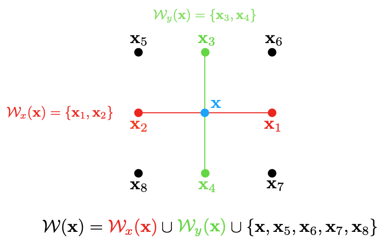
The vector $(s({\bf x}),s({\bf x}_{1}),s({\bf x}_{2}),s({\bf x}_{3}),s({\bf x}_{4}))$ is first properly detrended by considering the trend $d=\frac{1}{3}(s({\bf x})+s({\bf x}_{1})+s({\bf x}_{2})+s({\bf x}_{3})+s({\bf x}_{4}))$ and generate from it the detrended vector $(s({\bf x})+d,s({\bf x}_{1})-d,s({\bf x}_{2})-d,s({\bf x}_{3})-d,s({\bf x}_{4})-d)$. Let us denote this detrended vector by $({p}_{0}({\bf x}),{p}_{1}({\bf x}),{p}_{2}({\bf x}),{p}_{3}({\bf x}),{p}_{4}({\bf x}))$. We define

$$\begin{array}[]{lcl}\varepsilon_{x}({\bf x})&=&\alpha(p_{2}({\bf x})-p_{1}({\bf x}))\\ \varepsilon_{y}({\bf x})&=&\alpha(p_{4}({\bf x})-p_{3}({\bf x}))\\ \end{array}$$ (44)

with $\alpha>0$. Note that the values of $\varepsilon_{x}({\bf x})$ and $\varepsilon_{y}({\bf x})$ are related to the ”cross” neighboring sets ${\cal W}_{x}({\bf x})$ and ${\cal W}_{y}({\bf x})$ shown in red and green in Fig. 27. The local correlation measure is then defined as:

$${\cal H}(\mu_{n},{\bf x},{\bf r}_{0})=\displaystyle\left(\left(\varepsilon_{x}({\bf x})^{2}+\varepsilon_{y}({\bf x})^{2}\right)\left(\frac{{\cal A}({\bf x},{\bf r}_{0})}{\displaystyle\mu_{n}({\cal W}({\bf x}))}\right)\right)^{1/2}$$ (45)

with

$${\cal A}({\bf x},{\bf r}_{0})=\displaystyle\left|\varepsilon_{x}({\bf x})\left(\sum_{{\bf y}\in{\cal W}({\bf x})}\varepsilon_{x}({\bf y})\right)+\varepsilon_{y}({\bf x})\left(\sum_{{\bf y}\in{\cal W}({\bf x})}\varepsilon_{y}({\bf y})\right)\right|.$$

The value ${\bf h}({\bf x})$ is then computed with equation 43. Once the singularity exponents are determined, they define the collection of sets ${\cal F}_{\bf h}=\{\leavevmode\nobreak\ {\bf x}\leavevmode\nobreak\ |\leavevmode\nobreak\ {\bf h}({\bf x})={\bf h}\leavevmode\nobreak\ \}$ which are of particular importance in the description of a turbulent system (Frisch 1995). In Turiel et al. (2008) an argument for the case of log-Poisson processes is derived, which generalizes the work presented in She & Leveque (1994), and which describes the multiplicative cascade from the geometrical organization of the level-sets ${\cal F}_{\bf h}$ defined by the local singularity exponents. However a general justification valid for a large class of physical processes is still being awaited.

Appendix C Cumulant Analysis Method

In this appendix we go back to the canonical description of multifractality, considering an advanced and powerful computational approach based on cumulants, which was introduced in Delour et al. (2001); it is used in this work as it provides a criterion to determine the existence of a multiplicative cascade (Arneodo et al. 1998, 1999b) and the existence of long-range correlations. The reader is referred to Venugopal et al. (2006a) for a detailed and accurate description. If $\mu$ is a probability measure on the line, its characteristic function is $f_{\mu}(z)={\operatorname*{\mathbb{E}}}_{\mu}(e^{iz})$ which can be expanded in a power series involving $\mu$’s moments $M_{n}$: $f_{\mu}(z)=\displaystyle\sum_{n=0}^{\infty}M_{n}\frac{(iz)^{n}}{n!}$ with $M_{n}=\int x^{n}\mbox{d}{\mu}(x)$. The cumulant generating function of $\mu$, $g_{\mu}(z)$, is the $\log$ of $\mu$’s characteristic function: $g_{\mu}(z)=\log f_{\mu}(z)$. Since $M_{0}=1$, $g_{\mu}(z)=\displaystyle\log\left(1+\left(\sum_{n=1}^{\infty}M_{n}\frac{(iz)^{n}}{n!}\right)\right)$ which can in turn be expanded into a power series $g_{\mu}(z)=\displaystyle\sum_{n=0}^{\infty}C_{n}\frac{(iz)^{n}}{n!}$; the $C_{n}$ are called the cumulants of $\mu$. The first cumulants are given by the following relations:

$$\begin{array}[]{lcl}C_{1}&=&M_{1}\\ C_{2}&=&M_{2}-M_{1}^{2}\\ C_{3}&=&M_{3}-3M_{2}M_{1}+2M_{1}^{3}\end{array}$$ (46)

and the general recurrence relation is:

$$C_{n}=M_{n}-\displaystyle\sum_{l=1}^{n-1}\left(\begin{array}[]{c}n-1\\ l-1\end{array}\right)C_{l}M_{n-l}.$$ (47)

The most interesting part of the theory is the relation between the $C_{n}$ and the multifractal spectrum when $\mu$ is a multifractal measure. We collect the main results here.
As in Sect. 3 let $s$ be a given signal, $\psi$ an analyzing wavelet, ${\cal T}_{\psi}({\bf x},{\bf r})$ the wavelet-projected signal evaluated at position ${\bf x}$ and scale ${\bf r}$, $Z(q,{\bf r})$ a suitably chosen $q$th order partition function built out of ${\cal T}_{\psi}$. Let us consider, as the analyzing measure $\mu$, the one having density $\log|{\cal T}_{\psi}({\bf x},{\bf r})|$. Let $C_{n}({\bf r})$ be its cumulants. Then the evaluation of the slope of $C_{n}({\bf r})$ vs $\log({\bf r})$ gives, when ${\bf r}\rightarrow 0$, coefficients:

$$C_{n}\sim(-1)^{n+1}c_{n}\log({\bf r})$$ (48)

in such a way that $\tau(q)$ can be retriewed as $\tau(q)=-c_{0}+c_{1}q-c_{2}q^{2}/2!+c_{3}q^{3}/3!+\cdots$. For a 1D $\log$-normal process, $c_{n}=0$ for $n>2$ and one has

$$D({\bf h})=c_{0}-\displaystyle\frac{({\bf h}-c_{1})^{2}}{2c_{2}}$$ (49)

i.e. we get a parabolic spectrum as stated before, and comparing with the previous general expression for the singularity spectrum of a $\log$-normal process (eq. 9 Sect. 3), we find in this case: $c_{0}=1$, (dimension of the support of the measure), $c_{1}={\bf h}_{m}$ (average value of the singularity exponents) and $c_{2}=\sigma_{{\bf h}}^{2}$ (variance).

Appendix D Two-point magnitude statistical analysis and the multiplicative cascade

Keeping up with the notation of the last section, we define the two-point correlation function for a given scale ${\bf r}$ and spatial interval $\Delta{\bf x}$:

$$\begin{array}[]{lcl}{\cal C}({\bf r},\Delta{\bf x})&=&\langle\,(\log|{\cal T}_{\psi}({\bf x},{\bf r})|-\langle\log|{\cal T}_{\psi}({\bf x},{\bf r})|\rangle\,)\cdot\\ \nobreak\leavevmode&\nobreak\leavevmode\hfil&(\log|{\cal T}_{\psi}({\bf x}+\Delta{\bf x},{\bf r})|-\langle\log|{\cal T}_{\psi}({\bf x},{\bf r})|\rangle\,)\,\rangle.\end{array}$$ (50)

It is shown that if ${\cal C}({\bf r},\Delta{\bf x})$ is logarithmic in $\Delta{\bf x}$ and independent of scale ${\bf r}$ provided $\Delta{\bf x}>{\bf r}$ i.e. ${\cal C}({\bf r},\Delta{\bf x})\sim\log\Delta{\bf x}$ then long-range dependence exists in the system (Arneodo et al. 1998; Venugopal et al. 2006a). If there is a multiplicative cascade, then

$${\cal C}({\bf r},\Delta{\bf x})\sim-c_{2}\log\Delta{\bf x}.$$ (51)

We note that some random processes can be self-similar without displaying a multiplicative cascade (Arneodo et al. 1999a, b; Venugopal et al. 2006a). This feature is often neglected in multifractal analysis of signals in astronomy, although it is of primary importance if one wants to prove the existence of a multiplicative cascade in the ISM.