Hydrodynamic collective modes in graphene

Abstract

Collective behavior is one of the most intriguing aspects of the hydrodynamic approach to electronic transport. Here we provide a consistent, unified calculation of the dispersion relations of the hydrodynamic collective modes in graphene. Taking into account viscous effects, we show that the hydrodynamic sound mode in graphene becomes overdamped at sufficiently large momentum scales. Extending the linearized theory beyond the hydrodynamic regime, we connect the diffusive hydrodynamic charge density fluctuations with plasmons.

Electronic hydrodynamics is quickly growing into a mature field of solid state physics [1, 2, 3, 4, 5, 6, 7, 8, 9, 10, 11, 12, 13, 14, 15, 16, 17]. Similarly to the usual hydrodynamics [18], this approach offers a universal, long-wavelength description of collective flows in interacting many-electron systems. Such flows have been experimentally confirmed [6] to be more efficient than the usual single-electron (ballistic or diffusive) transport.

In graphene, hydrodynamic collective modes have been considered by many authors [2, 19, 20, 21, 15, 22, 23, 24, 25, 26]. All of them agree that at charge neutrality, the ideal electronic fluid (i.e., neglecting all dissipative processes) allows for a sound-like collective mode (which has been referred to as either the “cosmic sound” [20] or the “second sound” [25]) with the dispersion relation

$$\omega=v_{g}q/\sqrt{2},$$ (1)

where $v_{g}$ is the quasiparticle velocity in graphene. Taking into account dissipation changes the above dispersion relation giving rise to damping. To the best of our knowledge, no consensus on the latter effect has been reached so far with several contradicting results available in the literature [15, 23].

The hydrodynamic approach to electronic systems is applicable in an intermediate parameter regime [1, 2]. In particular, the underlying gradient expansion is valid at length scales much larger than the typical length scale $\ell_{ee}$ describing the energy- and momentum-conserving interaction (responsible for equilibration of the system). At smaller length scales, one can study more traditional collective excitations in interacting many-electron systems, including plasmons [15, 27, 24, 25, 26, 28, 29, 30, 31, 21, 32, 33, 34, 35, 36, 37, 38, 39, 40, 41, 42], which behavior is well established both theoretically and experimentally.

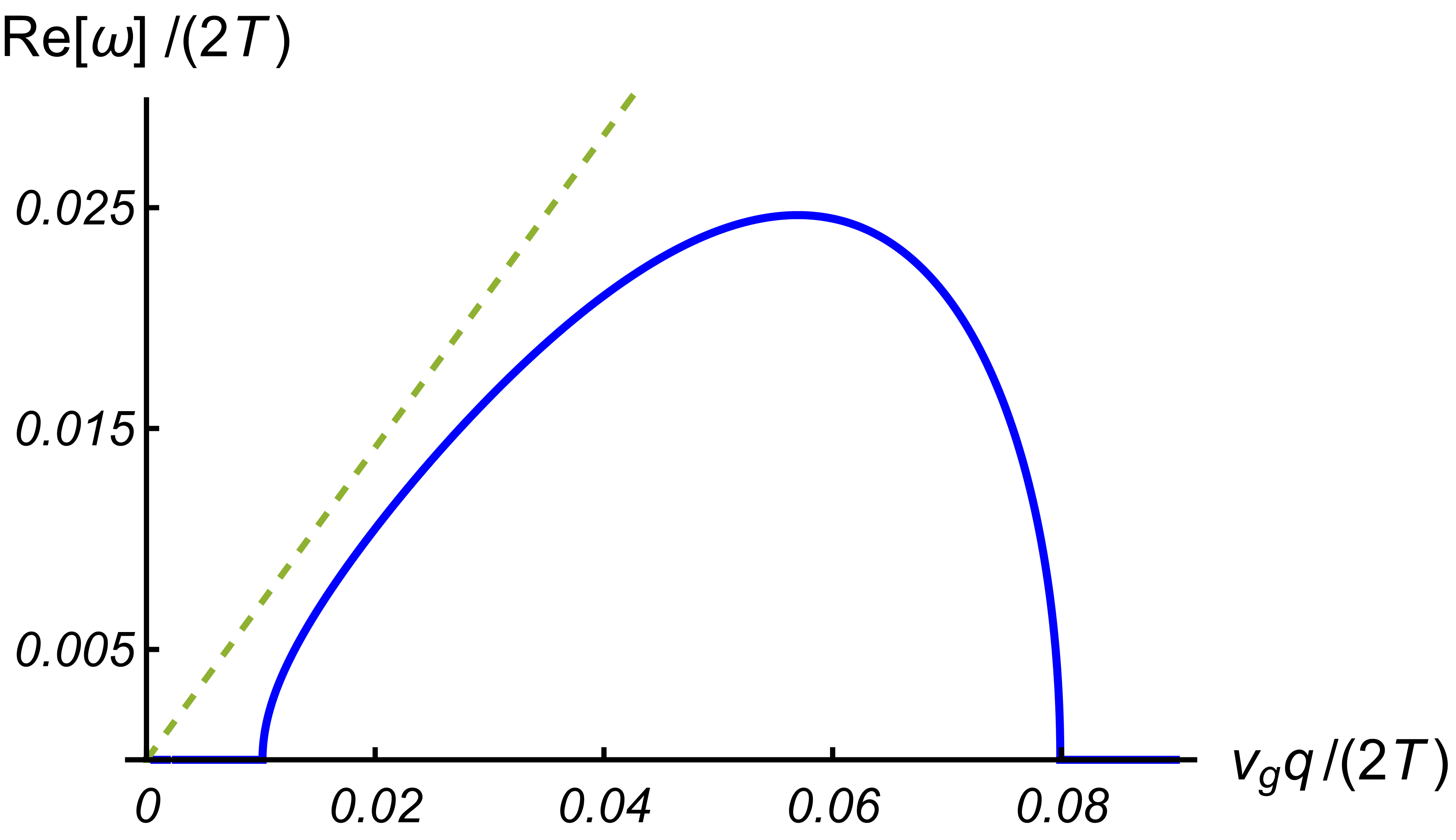
Figure 1: Real (top) and imaginary (bottom) parts of the hydrodynamic sound dispersion in neutral graphene taking into account viscosity and weak disorder, Eq. (2). The numerical values were computed with the realistic parameter values taken from Refs. 3, 9, 12; see the main text. The dispersion acquires a finite real part at the threshold value of momentum determined by dissipation. The mode becomes overdamped at small enough momenta, still in the region of the growing real part. The dashed line shows the ideal dispersion, Eq. (1).

In this paper we provide a consistent, unified calculation of the dispersion relations of the hydrodynamic collective modes in graphene. While the true hydrodynamics is universal (as long as no symmetries are broken), graphene is somewhat unique in the sense that there are two length scales associated with electron-electron interaction that are parametrically different in the weak coupling limit [43, 2, 44, 25]. This allows us to extend the results of the linearized hydrodynamic theory [43, 15, 45] to the length scales smaller that $\ell_{ee}$ (going beyond the small-momentum expansion of Ref. 15). At that point the sound mode (1) in neutral graphene (see Fig. 1) becomes overdamped due to the high viscosity [3, 9, 46]

$$\omega=\sqrt{\frac{v_{g}^{2}q^{2}}{2}-\frac{\left(1\!+\!q^{2}\ell_{G}^{2}\right)^{2}}{4\tau^{2}_{{\rm dis}}}}-i\frac{1\!+\!q^{2}\ell_{G}^{2}}{2\tau_{{\rm dis}}},$$ (2)

where $\tau_{\rm dis}$ is the disorder mean free time and $\ell_{G}$ is the so-called Gurzhi length [47, 48, 49, 50, 51] (here $\nu$ stands for the kinematic viscosity [2, 3, 9, 46])

$$\ell_{G}=\sqrt{\nu\tau_{\rm dis}}.$$ (3)

This mode describes energy fluctuations and is completely decoupled from charge fluctuations. The latter are purely diffusive within the hydrodynamic approach, where dissipation is described by the momentum- and frequency-independent coefficients, including the electrical conductivity and viscosity.

Extending the linearized theory beyond the hydrodynamic regime, we are able to connect the charge fluctuations with the more conventional plasmons by taking into account the frequency and momentum dependence of conductivity. At charge neutrality we find the plasmon mode

$$\omega=\sqrt{\frac{v_{g}^{2}\varkappa q}{2}\left(1\!+\!\frac{q}{\varkappa}\right)-\frac{v_{g}^{4}\varkappa^{2}}{64\pi^{2}\sigma_{0}^{2}}}-i\frac{v_{g}^{2}\varkappa}{8\pi\sigma_{0}},$$ (4)

where $\sigma_{0}$ is the conductivity in neutral graphene [1, 2, 16, 52]

$$\sigma_{0}=\frac{2e^{2}T\ln 2}{\pi}\frac{\tau_{11}\tau_{\rm dis}}{\tau_{11}\!+\!\tau_{\rm dis}},$$ (5)

and $\varkappa$ is the inverse Thomas-Fermi screening length. Neglecting dissipation and for small momenta, the dispersion (4) coincides with the result of Ref. 19.

Finally, we extend our results over the whole range of carrier densities up to the degenerate (“Fermi-liquid”) regime. Given the weak density dependence of the kinematic viscosity in graphene [3, 9, 46] the sound dispersion remains qualitatively similar to that shown in Fig. 1 at all doping levels.

I Hydrodynamic theory of electronic transport in graphene

In this Section, we briefly review the hydrodynamic theory of electronic transport in graphene.

I.1 Nonlinear hydrodynamic equations

The complete set of hydrodynamic equations includes the generalized Navier-Stokes equation [16, 17]

$$\!\!\!\!\!\!W(\partial_{t}+\boldsymbol{u}\!\cdot\!\boldsymbol{\nabla})\boldsymbol{u}+v_{g}^{2}\boldsymbol{\nabla}P+\boldsymbol{u}\partial_{t}P+e(\boldsymbol{E}\!\cdot\!\boldsymbol{j})\boldsymbol{u}=$$ (6a)

$$=v_{g}^{2}\left[\eta\Delta\boldsymbol{u}-\eta_{H}\Delta\boldsymbol{u}\!\times\!\boldsymbol{e}_{B}+en\boldsymbol{E}+\frac{e}{c}\boldsymbol{j}\!\times\!\boldsymbol{B}\right]-\frac{W\boldsymbol{u}}{\tau_{{\rm dis}}},$$

the continuity equations [1, 2, 16]

$$\partial_{t}n+\boldsymbol{\nabla}\!\cdot\!\boldsymbol{j}=0,$$ (6b)

$$\partial_{t}n_{I}+\boldsymbol{\nabla}\!\cdot\!\boldsymbol{j}_{I}=-\frac{n_{I}\!-\!n_{I,0}}{\tau_{R}},$$ (6c)

and the generalized “heat transport” equation [53, 54, 55] (we follow the usual approach [18] using the entropy flow equation instead of the continuity equation for energy).

$$T\left[\frac{\partial s}{\partial t}+\boldsymbol{\nabla}\!\cdot\!\frac{3P\boldsymbol{u}-\mu\boldsymbol{j}-\mu_{I}\boldsymbol{j}_{I}}{T}\right]=$$ (6d)

$$\qquad\qquad=\delta\boldsymbol{j}\!\cdot\!\left[e\boldsymbol{E}\!+\!\frac{e}{c}\boldsymbol{u}\!\times\!\boldsymbol{B}\!-\!T\boldsymbol{\nabla}\frac{\mu}{T}\right]-T\delta\boldsymbol{j}_{I}\!\cdot\!\boldsymbol{\nabla}\frac{\mu_{I}}{T}$$

$$\qquad\qquad\qquad+\frac{\eta}{2}\left(\nabla_{\alpha}u_{\beta}\!+\!\nabla_{\beta}u_{\alpha}\!-\!\delta_{\alpha\beta}\boldsymbol{\nabla}\!\cdot\!\boldsymbol{u}\right)^{2}$$

$$\qquad\qquad\qquad-\frac{n_{E}\!-\!n_{E,0}}{\tau_{RE}}+\mu_{I}\frac{n_{I}\!-\!n_{I,0}}{\tau_{R}}+\frac{W\boldsymbol{u}^{2}}{v_{g}^{2}\tau_{\rm dis}}.$$

Here $\boldsymbol{u}$ is the hydrodynamic velocity, $c$ is the speed of light, and $n$ and $n_{I}$ are the carrier and imbalance densities ($n_{I,0}$ is the equilibrium value), related to the quasiparticle densities in each of the two bands by

$$n=n_{+}-n_{-},\qquad n_{I}=n_{+}+n_{-}.$$

The carrier density $n$ differs from the charge density by a multiplicative factor of the electric charge, $e$. Similarly, we define the two quasiparticle currents, $\boldsymbol{j}$ and $\boldsymbol{j}_{I}$,

$$\boldsymbol{j}=\boldsymbol{j}_{+}-\boldsymbol{j}_{-},\qquad\boldsymbol{j}_{I}=\boldsymbol{j}_{+}+\boldsymbol{j}_{-},$$

with the electric current $\boldsymbol{J}=e\boldsymbol{j}$. We also define the two chemical potentials, $\mu$ and $\mu_{I}$,

$$\mu=(\mu_{+}+\mu_{-})/2,\qquad\mu_{I}=(\mu_{+}-\mu_{-})/2,$$

allowing for the two independent chemical potentials for each band out of equilibrium [53] (hence the term “imbalance”). The remaining vector quantities in Eqs. (6) are the electric field $\boldsymbol{E}$ and the magnetic field $\boldsymbol{B}$. The thermodynamic quantities are the enthalpy density $W$, pressure $P$, entropy density $s$, and temperature $T$. Finally, $\eta$ and $\eta_{H}$ are the shear and Hall viscosities, $\tau_{R}$ is the recombination time [53] [the recombination term in Eq. (6c) agrees with Ref. 54, whereas Ref. 53 suggests a slightly different term that is proportional to $\mu_{I}$ instead of the $\delta n_{I}$], and $\tau_{RE}$ is the energy relaxation time [55]. In equilibrium, $\mu_{I}=0$.

In comparison to the usual hydrodynamics [18], the electronic system in graphene is characterized by one additional variable describing the second band. Traditional ideal fluid is described by two thermodynamic variables, e.g., density and pressure, and the velocity field. As a result, in two dimensions one needs four equations to describe the dynamics of the flow. Two of these are given by the Euler equation, the third is the continuity equation, while the fourth can be either the continuity equation for energy or the adiabaticity equation (i.e., the continuity equation for entropy). In graphene these are Eqs. (6a), (6b), and (6d) in the absence of dissipation. The additional continuity equation (6c) for the quasiparticle density $n_{I}$ appears exactly due to the presence of the second band, which is why the overall number of hydrodynamic equations as well as independent variables in graphene is five. As the additional variable one can choose either $n_{I}$ or the corresponding chemical potential $\mu_{I}$.

The entropy flow equation (6d) should be compared to the corresponding equations in Refs. 2, 53, 54. The four equations contain mostly the same terms (up to trivial notation changes) with the following exceptions. Equation (54) of Ref. 2 is written in the relativistic notation omitting the imbalance mode, quasiparticle recombination, and disorder scattering, all of which are discussed separately elsewhere in Ref. 2. Reference 53 was the first to focus on the imbalance mode with Eq. (2.6) containing all the terms of Eq. (6d) except for the viscous term. Finally, Eq. (1c) of Ref. 54 contains all of the terms in Eq. (6d) and in addition contains a term describing energy relaxation due to electron-phonon scattering that is neglected in this paper (generalization of the resulting theory is straightforward).

Weak disorder scattering is described in Eqs. (6a) and (6d) by the mean free time $\tau_{\rm dis}$. The disorder contribution to the hydrodynamic equations was derived in Ref. 16 using the simplest $\tau$-approximation to the kinetic equation. A better version of the disorder collision integral in graphene should involve the Dirac factors suppressing backscattering [56] which would lead to the similar approximation but with the transport scattering time. In graphene, this brings about a factor of $2$. In this paper, we treat $\tau_{\rm dis}$ as a phenomenological parameter adopting the approach of Ref. 12.

The imbalance density $n_{I}$ appears under the assumption of the approximate conservation of the number of particles in each individual band. The processes that break this conservation (i.e., mix electrons and holes) involve the three-particle scattering, Auger processes [53], and most importantly, impurity assisted electron-phonon coupling [57]. These effects are described in Eq. (6c) by the phenomenological [58, 59] recombination time [60], $\tau_{R}$, as well as the energy relaxation time $\tau_{RE}$ in Eq. (6d).

I.2 Dissipative corrections to quasiparticle currents

The usual hydrodynamic flow [18] is a mass flow where dissipative processes lead to a correction to the energy flux as described by the thermal conductivity. Consequently the flow is characterized by three dissipative coefficients, the thermal conductivity $\varkappa$ and two viscosities $\eta$ and $\zeta$. In contrast, electronic hydrodynamics in graphene describes an energy flow where the quasiparticle currents acquire dissipative corrections. The energy flow is proportional to the momentum density and hence can only be affected by disorder, which is “extrinsic” to the hydrodynamic theory. As a result, the dissipative coefficients include the electrical conductivity $\sigma$ and viscosity, while the thermal conductivity has to be computed by solving the linear response equations (similarly to the electrical conductivity in the standard theory). Within the three-mode approximation of Ref. 16, the bulk viscosity vanishes, ${\zeta=0}$. In the absence of the magnetic field the dissipative corrections are related to external bias by means of a “conductivity matrix” [16, 53, 54]

$$\begin{pmatrix}\delta\boldsymbol{j}\cr\delta\boldsymbol{j}_{I}\end{pmatrix}=\widehat{\Sigma}\begin{pmatrix}e\boldsymbol{E}-T\boldsymbol{\nabla}(\mu/T)\cr-T\boldsymbol{\nabla}(\mu_{I}/T)\end{pmatrix}.$$ (7)

In particular, at the Dirac point ${\mu=\mu_{I}=0}$ the matrix $\widehat{\Sigma}$ is diagonal with the upper diagonal element defining (in the absence of disorder) the “quantum” or “intrinsic” conductivity [16, 2, 1, 53, 54]

$$\sigma_{Q}=e^{2}\Sigma_{11}(0).$$ (8)

In the hydrodynamic theory of graphene, the elements of the matrix $\widehat{\Sigma}$ play the role that is equivalent to that of the thermal conductivity $\varkappa$ in the usual hydrodynamics. The matrix nature of $\widehat{\Sigma}$ reflects the band structure of graphene. In the case of strong recombination, the imbalance mode becomes irrelevant and one is left with the single dissipative coefficient $\sigma_{Q}$, see Ref. 2.

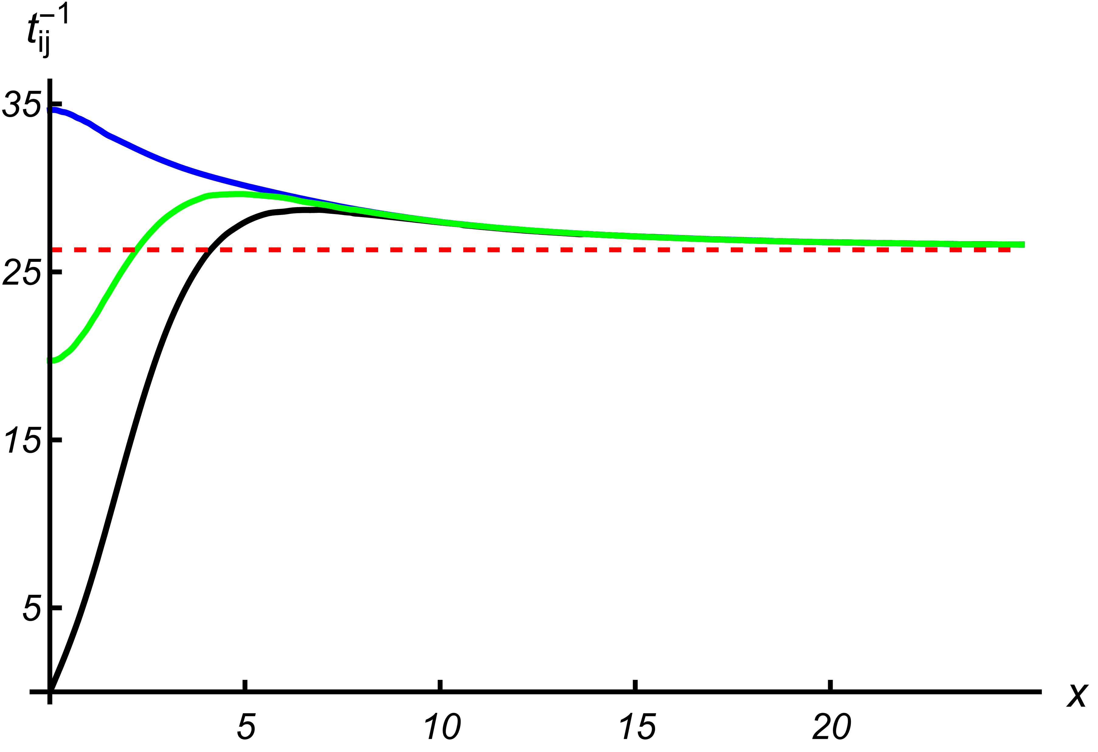
Figure 2: Dimensionless scattering rates comprising the matrix $\widehat{\textswab{T}}$: $t_{11}^{-1}$, $t_{12}^{-1}$, $t_{22}^{-1}$ (blue, black, and green, respectively). The red dashed line indicates the “Fermi-liquid” limit, Eq. (11).

I.2.1 Macroscopic currents within the three-mode approximation

Within the three-mode approximation of Ref. 16, one defines three macroscopic currents (using $\bar{W}=3\bar{n}_{E}/2$)

$$\boldsymbol{j}=\bar{n}\boldsymbol{u}\!+\!\delta\boldsymbol{j},\quad\boldsymbol{j}_{I}=\bar{n}_{I}\boldsymbol{u}\!+\!\delta\boldsymbol{j}_{I},\quad\boldsymbol{j}_{E}=\frac{3}{2}\bar{n}_{E}\boldsymbol{u},$$ (9)

where $\bar{n}$, $\bar{n}_{I}$, and $\bar{n}_{E}$ are the equilibrium values of the carrier, imbalance, and energy densities, respectively. The linear response theory relates the dissipative corrections $\delta\boldsymbol{j}$ and $\delta\boldsymbol{j}_{I}$ to the external bias by Eq. (7). The dimensionless conductivity matrix (at ${\boldsymbol{B}=0}$) is given by [16]

$$\widehat{\Sigma}=\widehat{\textswab{M}}\,\widehat{\textswab{S}}_{xx}^{-1}\widehat{\textswab{M}},\quad\widehat{\textswab{S}}_{xx}=\frac{\alpha_{g}^{2}T^{2}}{2{\cal T}^{2}}\widehat{\textswab{T}}+\frac{\pi}{{\cal T}\tau_{\rm dis}}\widehat{\textswab{M}},$$ (10a)

where

$$\widehat{\textswab{M}}\!=\!\begin{pmatrix}1\!-\!\frac{2\tilde{n}^{2}}{3\tilde{n}_{E}}\frac{T}{\cal T}&\frac{xT}{\cal T}\!-\!\frac{2\tilde{n}\tilde{n}_{I}}{3\tilde{n}_{E}}\!\frac{T}{\cal T}\cr\frac{xT}{\cal T}\!-\!\frac{2\tilde{n}\tilde{n}_{I}}{3\tilde{n}_{E}}\frac{T}{\cal T}&1\!-\!\frac{2\tilde{n}_{I}^{2}}{3\tilde{n}_{E}}\frac{T}{\cal T}\end{pmatrix}\!,$$ (10b)

with dimensionless densities [see Eq. (15a) below]

$$\tilde{n}={\rm Li}_{2}\left(-e^{-x}\right)-{\rm Li}_{2}\left(-e^{x}\right)\!,\quad\tilde{n}_{I}=x^{2}/2+\pi^{2}/6,$$

$$\tilde{n}_{E}=-{\rm Li}_{3}\left(-e^{x}\right)-{\rm Li}_{3}\left(-e^{-x}\right)\!,$$ (10c)

$$x=\mu/T,\quad{\cal T}=2T\ln\left[2\cosh(x/2)\right],$$

and dimensionless scattering rates

$$\widehat{\textswab{T}}=\begin{pmatrix}t_{11}^{-1}&t_{12}^{-1}\cr t_{12}^{-1}&t_{22}^{-1}\end{pmatrix},\qquad t_{ij}^{-1}=\frac{8\pi{\cal T}}{\alpha_{g}^{2}NT^{2}}\tau_{ij}^{-1},$$ (10d)

where $\tau_{ij}^{-1}$ are the scattering rates that can be obtained by solving the kinetic equation within the three-mode approximation [15, 16, 44, 25]. The zeros in the matrix (10d) are the manifestation of energy and momentum conservation, which is also responsible for the vanishing dissipative correction to the energy current in the absence of the magnetic field [16]. The three dimensionless elements of the matrix $\widehat{\textswab{T}}$ are shown in Fig. 2 as a function of $x=\mu/T$.

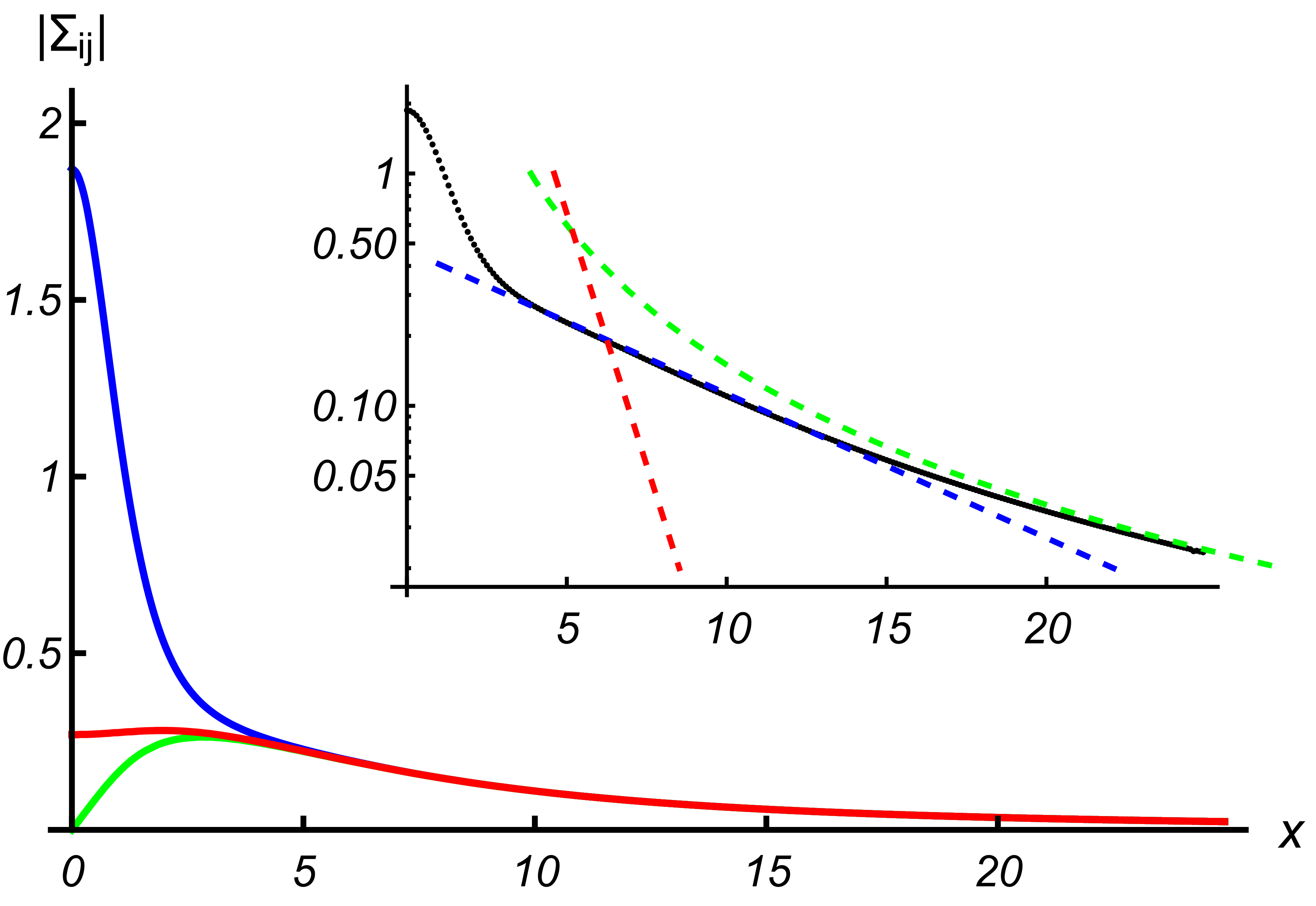
Figure 3: Matrix elements of $\widehat{\Sigma}$. The blue, red, and green curves correspond to $\Sigma_{11}$, $|\Sigma_{12}|$, $|\Sigma_{22}|$, respectively (notice, that ${\Sigma_{21}=-\Sigma_{12}}$). The inset shows the log plot of $\Sigma_{11}$, where the red and blue lines indicate the exponential decay, while the green line is the power law $\sim x^{-2}$.

The resulting matrix elements of the conductivity $\widehat{\Sigma}$ are shown in Fig. 3 as functions of $x=\mu/T$. As discussed below, the numerical precision of the present calculation is insufficient to track the exponential corrections to the scattering rates in the degenerate regime. Hence, the decay shown in the inset in Fig. 3 might be an artifact.

I.2.2 Dimensionless scattering rates

In the degenerate regime all scattering rates (i.e., the matrix elements $t_{ij}^{-1}$) coincide (up to exponentially small corrections) approaching the limiting value

$$t_{ij}^{-1}(\mu\gg T)\rightarrow 8\pi^{2}/3.$$ (11)

At $\mu=0$, the off-diagonal elements $t_{12}^{-1}(0)=0$, while the diagonal elements $t_{ii}^{-1}(0)$ determine the diagonal elements of the conductivity matrix, $\sigma_{Q}$ and $\sigma_{I}$, see below. For small $x\ll 1$ the dimensionless “scattering rates” $t_{ij}$ have the form [45] (see Fig. 4 for illustration)

$$\frac{1}{t_{11}}=\frac{1}{t_{11}^{(0)}}+x^{2}\!\left(\frac{1}{t_{11}^{(2)}}\!-\!\frac{1}{8\ln 2}\frac{1}{t_{11}^{(0)}}\right)\!+{\cal O}(x^{3}),$$ (12a)

$$\frac{1}{t_{12}}=\frac{x}{t_{12}^{(1)}}+{\cal O}(x^{3}),$$ (12b)

$$\frac{1}{t_{22}}=\frac{1}{t_{22}^{(0)}}+x^{2}\!\left(\frac{1}{t_{22}^{(2)}}\!-\!\frac{1}{8\ln 2}\frac{1}{t_{22}^{(0)}}\right)\!+{\cal O}(x^{3}).$$ (12c)

For unscreened Coulomb interaction, the dimensionless quantities $t_{ij}^{(0,1,2)}$ are just numbers without any dependence on any physical parameter. Numerically, one finds the following values (neglecting the small [52] exchange contribution):

$$\left(t_{11}^{(0)}\right)^{-1}\approx 34.63,\quad\left(t_{11}^{(2)}\right)^{-1}\approx 5.45,$$

$$\left(t_{12}^{(1)}\right)^{-1}\approx 5.72,\quad\left(t_{22}^{(0)}\right)^{-1}\approx 19.73,\quad\left(t_{22}^{(2)}\right)^{-1}\approx 5.65.$$

Note that these values are slightly different from those listed in Ref. 45. The reason for this is the use of different numerical methods. In the case of screened interaction, the quantities $t_{ij}^{(0,1,2)}$ depend on the screening length.

I.2.3 Conductivity matrix close to charge neutrality

Close to charge neutrality we expand the matrix $\widehat{\textswab{M}}$

$$\widehat{\textswab{M}}=\widehat{\textswab{M}}(0)+\delta\widehat{\textswab{M}}+{\cal O}(x^{3}),$$

with

$$\widehat{\textswab{M}}(0)=\begin{pmatrix}1&0\cr 0&\delta_{I}\end{pmatrix}\!,$$ (13)

where $\zeta(z)$ is the Riemann’s zeta function and

$$\delta_{I}=1-\frac{\pi^{4}}{162\zeta(3)\ln 2}\approx 0.28.$$

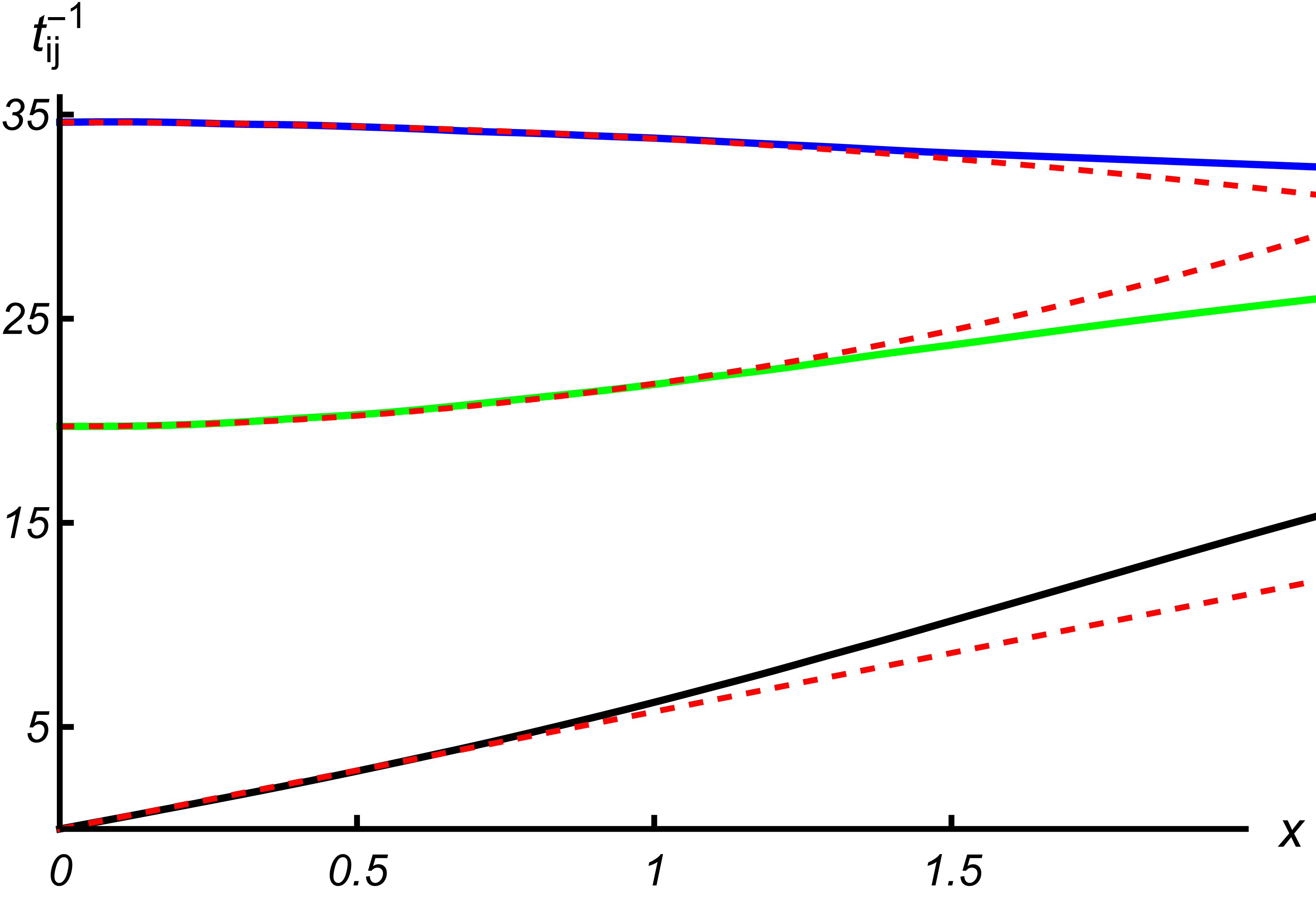
Figure 4: Dimensionless scattering rates close to charge neutrality. The blue, black, and green curves correspond to $t_{11}^{-1}$, $t_{12}^{-1}$, $t_{22}^{-1}$, respectively. The red dashed lines indicate the leading behavior close to charge neutrality (11).

The leading-order correction is given by

$$\!\!\!\!\!\delta\widehat{\textswab{M}}=\frac{x}{54\zeta(3)\ln 2}$$

$$\times\!\begin{pmatrix}-16x\ln^{2}2&27\zeta(3)\!-\!4\pi^{2}\!\ln 2\cr 27\zeta(3)\!-\!4\pi^{2}\!\ln 2&2\pi^{2}x\!\left[\frac{\pi^{2}}{48\ln 2}\!+\!\frac{\pi^{2}\!\ln 2}{9\zeta(3)}\!-\!1\right]\end{pmatrix}\!.$$

The matrix $\widehat{\textswab{S}}_{xx}$ can be expanded in the same way, using the expansion of the scattering rates (12):

$$\widehat{\textswab{S}}_{xx}=\widehat{\textswab{S}}_{xx}(0)+\delta\widehat{\textswab{S}}_{xx}+{\cal O}(x^{3}),$$

where

$$\widehat{\textswab{S}}_{xx}(0)\!=\!\frac{\pi}{2T\ln 2}\!\left[\!\begin{pmatrix}\tau_{11}^{-1}&0\cr 0&\tau_{22}^{-1}\end{pmatrix}\!+\!\frac{1}{\tau_{\rm dis}}\widehat{\textswab{M}}\right]\!,$$ (14)

and

$$\delta\widehat{\textswab{S}}_{xx}=\frac{\alpha_{g}^{2}}{8\ln^{2}2}\delta\widehat{\textswab{T}}+\frac{\pi}{2T\ln 2}\tau_{\rm dis}^{-1}\delta\widehat{\textswab{M}},$$

with

$$\delta\widehat{\textswab{T}}=x\begin{pmatrix}\frac{x}{t_{11}^{(2)}}\!-\!\frac{1}{8\ln 2}\frac{x}{t_{11}^{(0)}}&1/t_{12}^{(1)}\cr 1/t_{12}^{(1)}&\frac{x}{t_{22}^{(2)}}\!-\!\frac{1}{8\ln 2}\frac{x}{t_{22}^{(0)}}\end{pmatrix}.$$

Combining the above matrices, one finds the leading corrections to the conductivity matrix in the vicinity of the Dirac point, see Fig. 5.

Figure 5: Matrix elements of the dimensionless conductivity $\widehat{\Sigma}$ for small $x=\mu/T$. The blue, green, and red curves correspond to $\Sigma_{11}$, $\Sigma_{21}$, $|\Sigma_{22}|$, respectively. The dashed lines indicate the leading behavior close to charge neutrality.

Equations (6) and (7) reviewed in this Section represent a close set of hydrodynamic equations describing the electronic flows in graphene in the intermediate (“hydrodynamic”) temperature window [1, 2]. So far, these equations were mostly studied within linear response (nonlinear phenomena were discussed, e.g., in Ref. 15). The hydrodynamic collective modes are also obtained by linearizing the hydrodynamic equations.

II Linearized hydrodynamic theory at ${\boldsymbol{B}=0}$

In this Section, we discuss the linearization of the hydrodynamic theory in graphene suitable for a discussion of the bulk collective modes in the absence of the magnetic field, which is the primary focus of this paper.

Within linear response one considers small deviations of hydrodynamic quantities from their equilibrium values. At equilibrium, the stationary fluid is characterized by vanishing macroscopic currents and homogeneous thermodynamic quantities. Equilibrium quantities are most conveniently expressed in terms of the equilibrium values of temperature and chemical potential:

$$\mu\!=\!\bar{\mu},\qquad T\!=\!\bar{T},\qquad\mu_{I}\!=\!0,\qquad x\!=\!\bar{\mu}/\bar{T},$$ (15a)

$$n=\bar{n}=\frac{N\bar{T}^{2}}{2\pi v_{g}^{2}}\tilde{n},\quad\quad n_{I}=\bar{n}_{I}=\frac{N\bar{T}^{2}}{2\pi v_{g}^{2}}\tilde{n}_{I},$$

$$P=\bar{P}=\frac{N\bar{T}^{3}}{2\pi v_{g}^{2}}\tilde{n}_{E},\quad W=3\bar{P},\quad s=\frac{3\bar{P}-\bar{\mu}\bar{n}}{\bar{T}}.$$

Finally, the electric potential is homogeneous as well

$$\varphi=\bar{\varphi},\quad\boldsymbol{E}=-\boldsymbol{\nabla}\bar{\varphi}=0,\quad\boldsymbol{j}=\boldsymbol{j}_{I}=\boldsymbol{j}_{E}=0.$$ (15b)

The values $\bar{\mu}$, $\bar{\varphi}$, and $\bar{T}$ are determined by the environment in which the system is placed or, in other words, by the boundary conditions.

Once the system is subjected to a weak external voltage and temperature gradient, the hydrodynamic velocity $\boldsymbol{u}$ acquires a nonzero value and thermodynamic quantities become inhomogeneous. To the lowest (linear) order, one introduces small inhomogeneous fluctuations of the equilibrium quantities (not all being independent)

$$\mu=\bar{\mu}+\delta\mu,\qquad T=\bar{T}+\delta T,\qquad\varphi=\bar{\varphi}+\delta\varphi,$$ (16a)

$$n=\bar{n}+\delta{n},\qquad n_{I}=\bar{n}_{I}+\delta{n}_{I},\qquad P=\bar{P}+\delta{P},$$ (16b)

as well as small values for those quantities that vanish in equilibrium

$$\boldsymbol{u},\qquad\mu_{I}.$$ (16c)

The macroscopic currents have the form (9). Within linear response, the nonequilibrium corrections (9) [in general given in Eq. (7)] may be expressed as

$$\begin{pmatrix}\delta\boldsymbol{j}\cr\delta\boldsymbol{j}_{I}\end{pmatrix}=\widehat{\Sigma}\begin{pmatrix}-e\boldsymbol{\nabla}\delta\zeta+x\boldsymbol{\nabla}\delta{T}\cr-\boldsymbol{\nabla}\mu_{I}\end{pmatrix}\!,$$ (16d)

where $\widehat{\Sigma}$ is evaluated at equilibrium and

$$\delta\zeta=\delta\varphi+\frac{1}{e}\delta\mu,$$ (16e)

is the electrochemical potential. Here we used the fact that $\mu_{I}$ and $\boldsymbol{\nabla}\delta{T}$ are both assumed to be small, so that their products, e.g., $\mu_{I}\boldsymbol{\nabla}\delta{T}$, have to be neglected.

The same corrections can be expressed in terms of the density fluctuations rather than the chemical potentials [15]

$$\begin{pmatrix}\delta\boldsymbol{j}\cr\delta\boldsymbol{j}_{I}\end{pmatrix}\!\!=\widehat{\Sigma}\!\begin{pmatrix}e\boldsymbol{E}\cr 0\end{pmatrix}\!-\frac{\bar{T}^{2}}{\cal T}\widehat{\Sigma}^{\prime}\!\begin{pmatrix}\boldsymbol{\nabla}\delta\tilde{n}\!-\!\frac{2\tilde{n}}{3\tilde{n}_{E}}\boldsymbol{\nabla}\delta\tilde{n}_{E}\cr\boldsymbol{\nabla}\delta\tilde{n}_{I}\!-\!\frac{2\tilde{n}_{I}}{3\tilde{n}_{E}}\boldsymbol{\nabla}\delta\tilde{n}_{E}\end{pmatrix}\!,$$ (16f)

with dimensionless fluctuations of the densities and pressure [cf. Eqs. (16a) and (16b)] defined as

$$\delta n=\frac{N\bar{T}^{2}}{2\pi v_{g}^{2}}\delta\tilde{n},\quad\delta n_{I}=\frac{N\bar{T}^{2}}{2\pi v_{g}^{2}}\delta\tilde{n}_{I},\quad\delta P=\frac{N\bar{T}^{3}}{2\pi v_{g}^{2}}\delta\tilde{n}_{E},$$ (16g)

the quantity ${\cal T}$ is related to the equilibrium compressibility [16, 45, 15, 43]

$$\frac{\partial\bar{n}}{\partial\bar{\mu}}=\frac{N{\cal T}}{2\pi v_{g}^{2}},\quad{\cal T}=2\bar{T}\ln 2\cosh\frac{\bar{\mu}}{2\bar{T}},$$ (16h)

and finally

$$\widehat{\Sigma}^{\prime}=\widehat{\textswab{M}}\,\widehat{\textswab{S}}_{xx}^{-1},\qquad\widehat{\Sigma}=\widehat{\Sigma}^{\prime}\,\widehat{\textswab{M}}.$$ (16i)

The expressions (16d) and (16f) are completely equivalent, however one has to be careful with the electric field. Indeed, electrical conductivity is typically measured as a response to the “total” electric field and not to the “external electric field.” The total electric field includes the so-called Vlasov self-consistency [16, 2, 1, 43, 15] taking into account the electric field induced by the density fluctuations. The latter can be obtained using Poisson’s equation

$$\boldsymbol{E}_{V}=-e\boldsymbol{\nabla}\!\int\!d^{2}r^{\prime}\frac{\delta n(\boldsymbol{r}^{\prime})}{|\boldsymbol{r}\!-\!\boldsymbol{r}^{\prime}|}.$$ (17a)

This relation simplifies in gated structures, where [60, 61]

$$\boldsymbol{E}_{V}=-\frac{e}{C}\boldsymbol{\nabla}\delta n(\boldsymbol{r}).$$ (17b)

Here ${C=\varepsilon/(4\pi d)}$ is the gate-to-channel capacitance per unit area, $d$ is the distance to the gate, and $\varepsilon$ is the dielectric constant. This approximation neglects the long-ranged (dipole-type) part of the Coulomb interaction (screened by the gate) and is valid as long as the charge density $n(\boldsymbol{r})$ varies on length scales much longer than $d$.

Linearizing the hydrodynamic equations (6) we find

$$\frac{3\bar{P}}{v_{g}^{2}}\partial_{t}\boldsymbol{u}+\boldsymbol{\nabla}\delta P=\eta\Delta\boldsymbol{u}+e\bar{n}\boldsymbol{E}-\frac{3\bar{P}\boldsymbol{u}}{v_{g}^{2}\tau_{{\rm dis}}},$$ (18a)

$$\partial_{t}\delta{n}+\bar{n}\boldsymbol{\nabla}\!\cdot\!\boldsymbol{u}+\boldsymbol{\nabla}\!\cdot\!\delta\boldsymbol{j}=0,$$ (18b)

$$\partial_{t}\delta{n}_{I}+\bar{n}_{I}\boldsymbol{\nabla}\!\cdot\!\boldsymbol{u}+\boldsymbol{\nabla}\!\cdot\!\delta\boldsymbol{j}_{I}=-\delta{n}_{I}/\tau_{R},$$ (18c)

$$2\partial_{t}\delta{P}+3\bar{P}\boldsymbol{\nabla}\!\cdot\!\boldsymbol{u}=-2\delta{P}/\tau_{RE}.$$ (18d)

Notice that the linearized “thermal transport” equation (18d) is completely equivalent (within linear response) to the continuity equation for the energy flow; see Refs. 1, 2, 43, 15, 16. The energy relaxation term in Eq. (18d) was derived in Ref. [55].

At this point one has to choose the set of independent variables. Based on the form of the linearized equations (18), one can choose $\delta{n}$, $\delta{n}_{I}$, and $\delta{P}$. Together with the two components of $\boldsymbol{u}$ one has five variables for five differential equations (18). This set was used in Ref. 43 to discuss collective modes in the electronic fluid.

An alternative choice based on the form of dissipative corrections (16d) may include $\delta\zeta$, $\mu_{I}$, and $\delta{T}$. These variables were chosen in Ref. 53 for the discussion of the role of the imbalance mode in thermoelectric effects. Indeed, using the thermodynamic relation [16, 2, 18, 53]

$$dP=nd\mu+n_{I}d\mu_{I}+sdT,$$ (19)

in the linearized Navier-Stokes equation (18a), one finds

$$\frac{3\bar{P}}{v_{g}^{2}}\!\left(\partial_{t}\!+\!\tau_{{\rm dis}}^{-1}\right)\boldsymbol{u}\!=\!\eta\Delta\boldsymbol{u}\!-\!e\bar{n}\boldsymbol{\nabla}\zeta\!-\!\bar{n}_{I}\boldsymbol{\nabla}\mu_{I}\!-\!\frac{3\bar{P}\!-\!\bar{n}\bar{\mu}}{\bar{T}}\boldsymbol{\nabla}\delta{T},$$ (20)

where we combine the electric and chemical potential into the electrochemical potential (16e). Given that the densities and pressure are given by known functions of the chemical potentials and temperature, see Eqs. (15a), it’s a matter of simple algebra to express the rest of Eqs. (18) in terms of $\delta\zeta$, $\mu_{I}$, and $\delta{T}$.

While the choice of the thermodynamic variables is a matter of taste, there is an important distinction between static and dynamic response [2]. Static linear response equations contain only the electrochemical potential $\zeta$. However, the dynamic part of Eq. (18d) contains the chemical potential only. Consequently, one has to be careful considering response functions that depend on time and spatial coordinates at the same time. In this case, an additional equation (17) describing Vlasov self-consistency has to be taken into account [15].

III Collective modes at ${\boldsymbol{B}=0}$

      

Figure 6: Real part of the sound dispersion in moderately doped, gated graphene in the presence of both weak disorder and viscosity. Left pane: results for $n=10^{12}\,$cm^-2. Right panel: same for $n=10^{11}\,$cm^-2. The right panel also shows the zero mode Eq. (38).

Collective modes in the electronic fluid were considered within the same approach in Ref. 15, see also Refs. 2, 62, 44. These are the eigenmodes of the linearized equations (18). The most convenient choice of variables for this task is the density-pressure variables, $\delta{n}$, $\delta{n}_{I}$, and $\delta{P}$, and the velocity $\boldsymbol{u}$. The dissipative corrections to the currents are given by Eq. (16f) and the electric field in Eq. (18a) is the total electric field.

Now, it is convenient to solve linear differential equations with the help of the Fourier transform. Using the standard convention

$$\boldsymbol{u}(t,\boldsymbol{r})=\int\frac{d\omega d\boldsymbol{q}}{(2\pi)^{3}}e^{-i\omega t+i\boldsymbol{q}\boldsymbol{r}}\boldsymbol{u}(\omega,\boldsymbol{q}),$$

we rewrite Eqs. (18) in the dimensionless form

$$\left(\!\tilde{\omega}\!+\!i\frac{1\!+\!\tilde{q}^{2}\tilde{\ell}_{G}^{2}}{\tilde{\tau}_{{\rm dis}}}\right)\tilde{n}_{E}\boldsymbol{\rm v}-\frac{1}{3}\tilde{\boldsymbol{q}}\delta\tilde{n}_{E}-\tilde{\boldsymbol{q}}\tilde{V}_{q}\frac{e\tilde{n}}{6}\delta\tilde{n}=\frac{i}{6}e\tilde{n}\boldsymbol{\cal E}_{0},$$ (21a)

$$\tilde{\omega}\delta\tilde{n}-\tilde{n}\tilde{\boldsymbol{q}}\!\cdot\!\boldsymbol{\rm v}-\frac{2\pi}{N}\tilde{\boldsymbol{q}}\!\cdot\!\delta\tilde{\boldsymbol{j}}=0,$$ (21b)

$$\left(\!\tilde{\omega}\!+\!\frac{i}{\tilde{\tau}_{R}}\right)\delta\tilde{n}_{I}-\tilde{n}_{I}\tilde{\boldsymbol{q}}\!\cdot\!\boldsymbol{\rm v}-\frac{2\pi}{N}\tilde{\boldsymbol{q}}\!\cdot\!\delta\tilde{\boldsymbol{j}}_{I}=0,$$ (21c)

$$\left(\!\tilde{\omega}\!+\!\frac{i}{\tilde{\tau}_{RE}}\right)\delta\tilde{n}_{E}-\frac{3}{2}\tilde{n}_{E}\tilde{\boldsymbol{q}}\!\cdot\!\boldsymbol{\rm v}=0,$$ (21d)

where

$$\tilde{\boldsymbol{q}}=v_{g}\boldsymbol{q}/(2\bar{T}),\quad\tilde{\omega}=\omega/(2\bar{T}),\quad\boldsymbol{\rm v}=\boldsymbol{u}/v_{g},$$ (22a)

$$\tilde{\tau}_{j}=2\bar{T}\tau_{j}\,\,(j={\rm dis},\,R,\,RE),\quad\boldsymbol{\cal E}_{0}=v_{g}\boldsymbol{E}_{0}\bar{T}^{-2},$$ (22b)

the dimensionless Gurzhi length is defined so that

$$\tilde{q}\tilde{\ell}_{G}=q\ell_{G},$$ (22c)

and the self-consistent Vlasov potential is given by

$$\tilde{V}_{q}=\frac{eN\bar{T}}{\pi v_{g}^{2}}V_{s},\qquad V_{s}(\boldsymbol{q})=\begin{cases}e/C,&\text{gated},\cr 2\pi e/q,&\text{Coulomb},\end{cases}$$ (22d)

Finally, the dimensionless form of the dissipative corrections to the macroscopic currents is given by

$$\begin{pmatrix}\delta\tilde{\boldsymbol{j}}\cr\delta\tilde{\boldsymbol{j}}_{I}\end{pmatrix}=\widehat{\Sigma}\begin{pmatrix}e\boldsymbol{\cal E}_{0}\!-\!i\tilde{\boldsymbol{q}}\tilde{V}_{q}\delta\tilde{n}\cr 0\end{pmatrix}-\frac{i\tilde{\boldsymbol{q}}\,\widehat{\Sigma}^{\prime}}{\ln 2\cosh\frac{x}{2}}\!\begin{pmatrix}\delta\tilde{n}\!-\!\frac{2\tilde{n}}{3\tilde{n}_{E}}\delta\tilde{n}_{E}\cr\delta\tilde{n}_{I}\!-\!\frac{2\tilde{n}_{I}}{3\tilde{n}_{E}}\delta\tilde{n}_{E}\end{pmatrix}\!.$$ (23)

The collective modes can now be found by analyzing the system of Eqs. (21). For convenience, it can be written in the matrix form

$$\begin{pmatrix}\tilde{\omega}\!+\!\frac{i2\pi\tilde{q}^{2}}{N}\!\!\left[\!\Sigma_{11}\tilde{V}_{q}\!+\!\frac{\Sigma^{\prime}_{11}}{\ln 2\cosh\frac{x}{2}}\!\right]&\frac{i2\pi\tilde{q}^{2}\Sigma^{\prime}_{12}}{N\ln 2\cosh\frac{x}{2}}&-\frac{i4\pi\tilde{q}^{2}}{3N}\frac{\Sigma^{\prime}_{11}\tilde{n}\!+\!\Sigma^{\prime}_{12}\tilde{n}_{I}}{\tilde{n}_{E}\ln 2\cosh\frac{x}{2}}&-\tilde{n}\tilde{\boldsymbol{q}}\cr\frac{i2\pi\tilde{q}^{2}}{N}\!\left[\Sigma_{21}\tilde{V}_{q}\!+\!\frac{\Sigma^{\prime}_{21}}{\ln 2\cosh\frac{x}{2}}\right]&\tilde{\omega}\!+\!\frac{i}{\tilde{\tau}_{R}}\!+\!\frac{i2\pi\tilde{q}^{2}\Sigma^{\prime}_{22}}{N\ln 2\cosh\frac{x}{2}}&-\frac{i4\pi\tilde{q}^{2}}{3N}\frac{\Sigma^{\prime}_{21}\tilde{n}\!+\!\Sigma^{\prime}_{22}\tilde{n}_{I}}{\tilde{n}_{E}\ln 2\cosh\frac{x}{2}}&-\tilde{n}_{I}\tilde{\boldsymbol{q}}\cr 0&0&\tilde{\omega}\!+\!\frac{i}{\tilde{\tau}_{RE}}&-\frac{3}{2}\tilde{n}_{E}\tilde{\boldsymbol{q}}\cr-\tilde{\boldsymbol{q}}\tilde{V}_{q}\frac{\tilde{n}}{6}&0&-\frac{\tilde{\boldsymbol{q}}}{3}&\left[\!\tilde{\omega}\!+\!i\frac{1+\tilde{q}^{2}\tilde{\ell}_{G}^{2}}{\tilde{\tau}_{{\rm dis}}}\!\right]\!\tilde{n}_{E}\end{pmatrix}\!\!\!\begin{pmatrix}\delta\tilde{n}\cr\delta\tilde{n}_{I}\cr\delta\tilde{n}_{E}\cr\boldsymbol{\rm v}\end{pmatrix}\!=\!\begin{pmatrix}\frac{2\pi e}{N}\Sigma_{11}\tilde{q}{\cal E}_{0}\cr\frac{2\pi e}{N}\Sigma_{21}\tilde{q}{\cal E}_{0}\cr 0\cr\frac{i}{6}e\tilde{n}\boldsymbol{\cal E}_{0}\end{pmatrix}\!\!.$$ (24)

Dispersion relations of the collective modes are given by the zeros of the determinant of the matrix in the left-hand side of (24)

$$\left[\tilde{\omega}+i\frac{1+\tilde{q}^{2}\tilde{\ell}_{G}^{2}}{\tilde{\tau}_{{\rm dis}}}\right]\!\!$$ (25)

$$\qquad\times\left\{\left[\tilde{\omega}\!+\!\frac{i}{\tilde{\tau}_{R}}\!+\!\frac{i2\pi\tilde{q}^{2}\Sigma^{\prime}_{22}}{N\ln 2\cosh\frac{x}{2}}\right]\!\!\left[\tilde{\omega}\!+\!\frac{i2\pi\tilde{q}^{2}}{N}\!\!\left(\!\Sigma_{11}\tilde{V}_{\tilde{\boldsymbol{q}}}\!+\!\frac{\Sigma^{\prime}_{11}}{\ln 2\cosh\frac{x}{2}}\right)\!\right]\!\!\left[\!\left(\tilde{\omega}\!+\!\frac{i}{\tilde{\tau}_{RE}}\right)\!\!\left(\tilde{\omega}\!+\!i\frac{1\!+\!\tilde{q}^{2}\tilde{\ell}_{G}^{2}}{\tilde{\tau}_{{\rm dis}}}\right)\!-\!\frac{\tilde{q}^{2}}{2}\right]\right.$$

$$\qquad\qquad-\frac{2\pi\tilde{q}^{2}\Sigma^{\prime}_{12}}{N\ln 2\cosh\frac{x}{2}}\left[\frac{\tilde{q}^{2}\tilde{V}_{\tilde{\boldsymbol{q}}}\tilde{n}}{6\tilde{n}_{E}}\left(\tilde{n}\frac{2\pi\tilde{q}^{2}\Sigma^{\prime}_{21}}{N\ln 2\cosh\frac{x}{2}}\!+\!\frac{\tilde{n}_{I}}{\tilde{\tau}_{RE}}\!-\!\frac{\tilde{n}_{I}}{\tilde{\tau}_{R}}\right)\right.$$

$$\qquad\qquad\qquad\qquad\qquad\qquad\qquad\qquad-\left.\frac{2\pi\tilde{q}^{2}}{N}\!\left(\Sigma_{21}\tilde{V}_{\tilde{\boldsymbol{q}}}\!+\!\frac{\Sigma^{\prime}_{21}}{\ln 2\cosh\frac{x}{2}}\right)\!\!\left[\!\left(\tilde{\omega}\!+\!\frac{i}{\tilde{\tau}_{RE}}\right)\!\!\left(\tilde{\omega}\!+\!i\frac{1\!+\!\tilde{q}^{2}\tilde{\ell}_{G}^{2}}{\tilde{\tau}_{{\rm dis}}}\right)\!-\!\frac{\tilde{q}^{2}}{2}\right]\!\right]$$

$$\qquad\qquad\left.-\frac{\tilde{q}^{2}\tilde{V}_{q}\tilde{n}^{2}}{6\tilde{n}_{E}}\left(\tilde{\omega}\!+\!\frac{i}{\tilde{\tau}_{RE}}\!+\!\frac{i2\pi\tilde{q}^{2}\Sigma^{\prime}_{11}}{N\ln 2\cosh\frac{x}{2}}\right)\!\!\left(\tilde{\omega}\!+\!\frac{i}{\tilde{\tau}_{R}}\!+\!\frac{i2\pi\tilde{q}^{2}\Sigma^{\prime}_{22}}{N\ln 2\cosh\frac{x}{2}}\right)\!\right\}=0.$$

The first line in Eq. (25) is the factor determining the dispersion of the transverse fluctuations of the velocity field. Under our assumptions this mode is completely decoupled from the rest of the system and remains diffusive for all values of the carrier density. This might change if one considers long-range disorder [63], where it was argued to induce vortical flow near charge neutrality.

The rest of the equation is best solved numerically. In Fig. 6 we present the results of a numerical calculation of the real part of the dispersion for the two values of the carrier density, $n=10^{12}\,$cm^-2 and $n=10^{11}\,$cm^-2. Equation (25) was solved using the typical values of the effective coupling constant [12, 64] $\alpha_{g}=0.23$, disorder scattering time [12] $\tau_{\rm dis}^{-1}=1\,$THz, kinematic viscosity [46, 3] $\nu=0.2\,$m²/s, and temperature $T=300\,$K. The result is qualitatively similar to that shown in Fig. 1, therefore we postpone the discussion until after we have considered the two limiting cases where the dispersion can be obtained analytically, see Eq. (2).

III.0.1 Collective modes in neutral graphene

At charge neutrality, the linearized equations (21) can be simplified using the fact that the “conductivity matrices” $\widehat{\Sigma}$ and $\widehat{\Sigma}^{\prime}$ are block-diagonal (here we take into account weak disorder)

$$\widehat{\Sigma}\!=\!\frac{1}{e^{2}}\!\begin{pmatrix}\sigma_{0}&0\cr 0&\sigma_{I}\delta_{I}\end{pmatrix}\!\!,\quad\widehat{\Sigma}^{\prime}\!=\!\frac{1}{e^{2}}\!\begin{pmatrix}\sigma_{0}&0\cr 0&\sigma_{I}\end{pmatrix}\!\!.$$ (26)

As a result, the dissipative corrections (23) simplify

$$\delta\tilde{\boldsymbol{j}}=\frac{1}{e}\sigma_{0}\boldsymbol{\cal E}-\frac{i\tilde{\boldsymbol{q}}\sigma_{0}}{e^{2}\ln 2}\delta\tilde{n},$$ (27a)

$$\delta\tilde{\boldsymbol{j}}_{I}=-\frac{i\tilde{\boldsymbol{q}}\sigma_{I}}{e^{2}\ln 2}\left(\delta\tilde{n}_{I}\!-\!\frac{2\pi^{2}}{27\zeta(3)}\delta\tilde{n}_{E}\right).$$ (27b)

Using the explicit form of the equilibrium quantities [16], we rewrite Eqs. (21) in the form

$$\tilde{\boldsymbol{q}}\delta\tilde{n}_{E}-\frac{9\zeta(3)}{2}\!\left(\!\tilde{\omega}\!+\!i\frac{1+\tilde{q}^{2}\tilde{\ell}_{G}^{2}}{\tilde{\tau}_{{\rm dis}}}\right)\boldsymbol{\rm v}=0,$$ (28a)

$$\left(\tilde{\omega}+i\frac{2\pi\tilde{q}^{2}\sigma_{0}}{e^{2}N\ln 2}\right)\!\delta\tilde{n}=\frac{2\pi\sigma_{0}}{eN}\tilde{\boldsymbol{q}}\!\cdot\!\boldsymbol{\cal E},$$ (28b)

$$\left(\!\tilde{\omega}\!+\!\frac{i}{\tilde{\tau}_{R}}\!+\!\frac{i2\pi\tilde{q}^{2}\sigma_{I}}{e^{2}N\ln 2}\right)\!\delta\tilde{n}_{I}\!-\!\frac{\pi^{2}}{6}\tilde{\boldsymbol{q}}\!\cdot\!\boldsymbol{\rm v}\!-\!\frac{i4\pi^{3}\tilde{q}^{2}\sigma_{I}\delta\tilde{n}_{E}}{27\zeta(3)Ne^{2}\ln 2}\!=\!0,$$ (28c)

$$2\left(\!\tilde{\omega}\!+\!\frac{i}{\tilde{\tau}_{RE}}\right)\!\delta\tilde{n}_{E}-\frac{9\zeta(3)}{2}\tilde{\boldsymbol{q}}\!\cdot\!\boldsymbol{\rm v}=0.$$ (28d)

Combining Eqs. (28a) and (28d) to exclude the velocity, one finds

$$\tilde{q}^{2}\delta\tilde{n}_{E}=2\left(\!\tilde{\omega}\!+\!i\frac{1+\tilde{q}^{2}\tilde{\ell}_{G}^{2}}{\tilde{\tau}_{{\rm dis}}}\right)\!\!\left(\!\tilde{\omega}\!+\!\frac{i}{\tilde{\tau}_{RE}}\right)\!\delta\tilde{n}_{E},$$

yielding the spectrum (2) [in dimensionless units; in Eq. (2) we have neglected weak energy relaxation]

$$\tilde{\omega}=\sqrt{\frac{\tilde{q}^{2}}{2}\!-\!\frac{1}{4}\!\left[\frac{1\!+\!\tilde{q}^{2}\tilde{\ell}_{G}^{2}}{\tilde{\tau}_{{\rm dis}}}\!-\!\frac{1}{\tilde{\tau}_{RE}}\right]^{2}}-i\frac{1\!+\!\tilde{q}^{2}\tilde{\ell}_{G}^{2}}{2\tilde{\tau}_{{\rm dis}}}-\frac{i}{2\tilde{\tau}_{RE}}.$$ (29)

In the absence of dissipation this is the so-called “cosmic sound” wave [2, 15, 20] with the linear dispersion (1).

Same conclusions can be reached using the general form Eq. (25). At charge neutrality, Eq. (25) factorizes

$$\left[\!\left(\!\tilde{\omega}\!+\!i\frac{1+\tilde{q}^{2}\tilde{\ell}_{G}^{2}}{\tilde{\tau}_{{\rm dis}}}\right)\!\!\left(\!\tilde{\omega}\!+\!\frac{i}{\tilde{\tau}_{RE}}\right)\!-\!\frac{\tilde{q}^{2}}{2}\right]\!\!\left[\tilde{\omega}+i\frac{1+\tilde{q}^{2}\tilde{\ell}_{G}^{2}}{\tilde{\tau}_{{\rm dis}}}\right]$$ (30)

$$\quad\times\left[\tilde{\omega}+\frac{i}{\tilde{\tau}_{R}}+\frac{2\pi i\tilde{q}^{2}\sigma_{I}}{Ne^{2}\ln 2}\right]\!\!\left[\tilde{\omega}\!+\!\frac{2\pi i\tilde{q}^{2}\sigma_{0}}{Ne^{2}}\left(\tilde{V}_{\tilde{\boldsymbol{q}}}\!+\!\frac{1}{\ln 2}\right)\right]=0.$$

Here the first factor yields the spectrum (29), the last factor describes the transverse fluctuations of the velocity field, while the remaining two correspond to the charge and imbalance modes.

The sound mode (29) is the energy wave not involving charge density fluctuations [since neither Eq. (28a) nor Eq. (28d) contains $\delta\tilde{n}$]. Consequently, the sound spectrum is not affected by the Vlasov self-consistency (17).

Other modes are diffusive. Since Eqs. (28a) and (28d) are independent of the density fluctuations $\delta\tilde{n}$ and $\delta\tilde{n}_{I}$, the diffusive modes can be read off Eqs. (28b) and (28c).

      

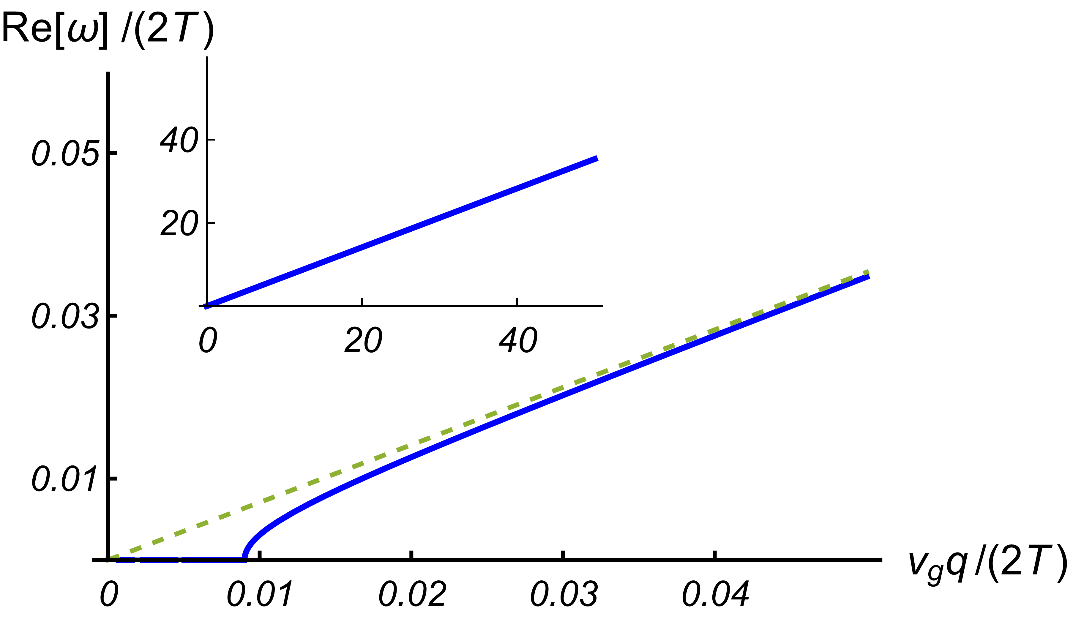
Figure 7: Real (left panel) and imaginary (right panel) parts of the sound dispersion in neutral graphene neglecting viscosity. The dashed line represents the ideal “cosmic sound” dispersion (1).

The electric charge density fluctuations are decoupled from the rest of the variables. Restoring the dimensionfull units and using the explicit form (5) of the conductivity at charge neutrality [16, 43, 1, 2, 52, 44, 62, 19, 65] we can write the corresponding dispersion as

$$\omega=-iD_{0}q^{2}\!\left[1\!+\!eV_{s}(q)\frac{\partial n}{\partial\mu}\right]\!,\quad D_{0}=\frac{1}{2}\frac{v_{g}^{2}\tau_{11}\tau_{\rm dis}}{\tau_{11}\!+\!\tau_{\rm dis}}.$$ (31)

In a gated structure the mode is diffusive with the diffusive coefficient containing a correction due to the Vlasov self-consistency. In the case of the long-range Coulomb interaction the dispersion is still purely imaginary, with $\omega\sim iq$ at small $q$.

Similarly, the imbalance mode is characterized by the diffusive spectrum

$$\omega=-iD_{I}q^{2}-\frac{i}{\tau_{R}},\quad D_{I}=\frac{1}{2}\frac{v_{g}^{2}\tau_{22}\tau_{\rm dis}\delta_{I}}{\tau_{22}\delta_{I}\!+\!\tau_{\rm dis}},$$ (32)

which is gapped by the recombination processes.

The hydrodynamic theory outlined in Section I is justified by the gradient expansion and hence for momenta smaller than a certain scale defined by the electron-electron interaction

$$q\ell_{\rm hydro}\ll 1,\quad\ell_{\rm hydro}\sim\frac{v_{g}}{\alpha_{g}^{2}\bar{T}}.$$

Assuming an ultra-clean sample with $\tau_{\rm dis}\rightarrow\infty$ (where energy relaxation due to supercollisions [55] may be neglected, $\tau_{RE}\gg\tau_{\rm dis}$), the expression under the square root in Eq. (29) yields

$$\frac{v_{g}^{2}q^{2}}{2}-\frac{\left(1\!+\!q^{2}\ell_{G}^{2}\right)^{2}}{4\tau^{2}_{{\rm dis}}}\rightarrow\frac{v_{g}^{2}q^{2}}{2}\left[1\!-\!Aq^{2}\ell_{\rm hydro}^{2}\!-{\cal O}(\tau_{\rm dis}^{-1})\right]\!,$$

where $A$ is a numerical coefficient. As a result, within the region of applicability of the hydrodynamic theory the viscous term should be neglected. The resulting dispersion acquires a simple form [15]

$$\omega=\sqrt{\frac{v_{g}^{2}q^{2}}{2}-\frac{1}{4\tau^{2}_{{\rm dis}}}}-\frac{i}{2\tau_{{\rm dis}}},$$ (33)

illustrated in Fig. 7. Now, keeping the viscous term to the leading order, but neglecting disorder scattering [23] yields an expansion

$$\omega=\frac{v_{g}q}{\sqrt{2}}\left(1-\frac{\nu^{2}q^{2}}{4v_{g}^{2}}\right)-\frac{i\nu q^{2}}{2}.$$ (34)

Similar expression was obtained in Ref. 23 based on the phenomenological collision integral (which did not take into account graphene-specific collinear scattering singularity). However, the viscosity-induced correction to the real part was positive indicating a tendency towards an indefinite growth of the dispersion instead of the decrease towards zero implied in Eqs. (1) and (29) and illustrated in Figs. 1 and 6. The sign of the correction in Eq. (34) is, in fact, dictated by the dissipative nature of viscosity, which represents an additional decay mechanism and hence affects the dispersion similarly to weak disorder; see Eq. (33). Indeed, both terms, $\tau_{\rm dis}^{-1}$ and ${\nu{q}^{2}}$, enter the dispersion equation [following from the first term in Eq. (30)] on equal footing.

As shown in Refs. 43, 15, 45, 66 the linearized theory (18) has a wider applicability range due to the kinematic peculiarity of the Dirac fermions in graphene known as the “collinear scattering singularity” [15, 44, 1, 2]. In the weak coupling limit, the linear response theory is valid at much shorter length scales

$$q\ell_{\rm coll}\ll 1,\quad\ell_{\rm coll}\sim\frac{v_{g}}{\alpha_{g}^{2}\bar{T}|\ln\alpha_{g}|}\ll\ell_{\rm hydro}.$$ (35)

At the same time, the viscous term is the result of the gradient expansion that is justified at smaller momenta

$$q\ell_{\rm hydro}\ll 1,$$

which formally restricts us to small values of $\nu q/v_{g}$, such that the result (29) should be expressed in terms of the expansion (34). Moreover, the imaginary part of the sound dispersion becomes comparable to the real part at $q\ell_{\rm hydro}\sim 1$, such that the decline of the dispersion at larger $q$ shown in Figs. 1 and 6 is unlikely to be observable anyway. Nevertheless in Figs. 1, 6, and 10 we show the sound dispersion in the whole range of momenta to illustrate the analytic structure of our results.

For realistic model parameters, the dispersion (29) shown in Figs. 1 and 6 is overdamped practically over the whole range of momenta. In the limit of large $\tau_{\rm dis}$ and small viscosity, the dispersion (29) approaches the ideal sound dispersion (1) if

$$(v_{g}\tau_{\rm dis})^{-1}\ll q\ll\ell_{G}^{-1}.$$

However, taking into account the numerical prefactors and realistic parameter values leads to Figs. 1 and 6, where the dispersion strongly deviates from Eq. (1).

      

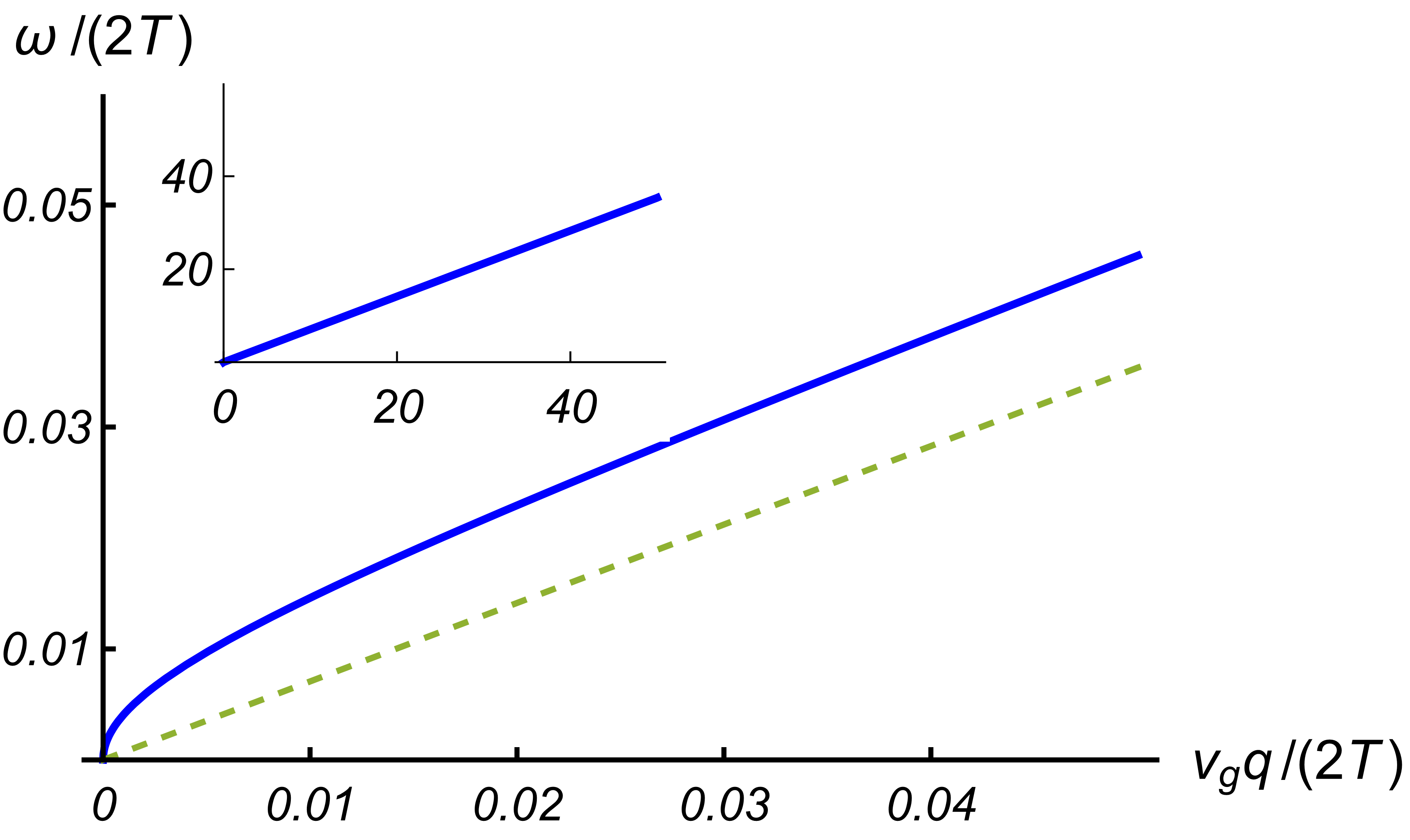
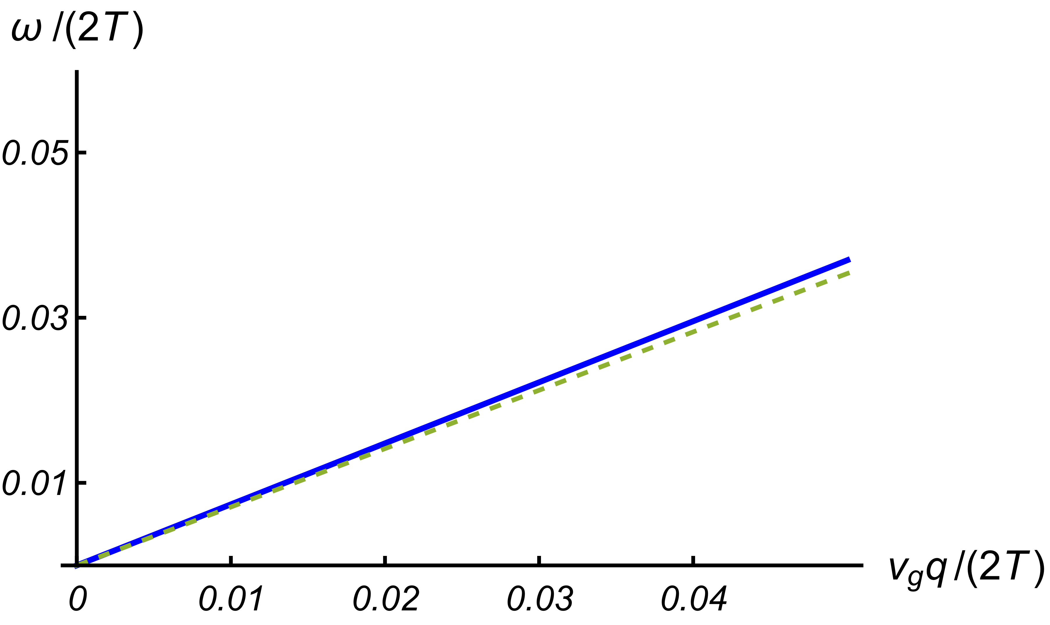
Figure 8: Sound dispersion in strongly doped graphene neglecting both weak disorder and viscosity. Left panel: the result for the Coulomb screening, resembling the 2D plasmon for very low $q$. Right panel: same for a gated structure. The dashed line represents the ideal “cosmic sound” dispersion (1).

III.0.2 Collective modes in the degenerate regime

In the opposite limit of the degenerate regime, ${\mu\gg{T}}$, the matrix in the left-hand side of Eq. (24) simplifies to

$$\begin{pmatrix}\tilde{\omega}&0&0&-\tilde{n}\boldsymbol{q}\cr 0&\tilde{\omega}\!+\!\frac{i}{\tilde{\tau}_{R}}&0&-\tilde{n}_{I}\boldsymbol{q}\cr 0&0&\tilde{\omega}\!+\!\frac{i}{\tilde{\tau}_{RE}}&-\frac{3}{2}\tilde{n}_{E}\boldsymbol{q}\cr-\boldsymbol{q}\tilde{V}_{q}\frac{e\tilde{n}}{6}&0&-\frac{\boldsymbol{q}}{3}&\left[\tilde{\omega}\!+\!i\frac{1+q^{2}\tilde{\ell}_{G}^{2}}{\tilde{\tau}_{{\rm dis}}}\right]\!\tilde{n}_{E}\end{pmatrix}\!,$$ (36)

such that Eq. (25) factorizes again

$$\left\{\tilde{\omega}\left[\left(\!\tilde{\omega}\!+\!i\frac{1+\tilde{q}^{2}\tilde{\ell}_{G}^{2}}{\tilde{\tau}_{{\rm dis}}}\right)\!\!\left(\!\tilde{\omega}\!+\!\frac{i}{\tilde{\tau}_{RE}}\right)\!-\!\frac{\tilde{q}^{2}}{2}\right]-\frac{\tilde{q}^{2}\tilde{V}_{q}e\tilde{n}^{2}}{6\tilde{n}_{E}}\left(\!\tilde{\omega}\!+\!\frac{i}{\tilde{\tau}_{RE}}\right)\right\}\left[\tilde{\omega}+\frac{i}{\tilde{\tau}_{R}}\right]\left[\tilde{\omega}+i\frac{1+\tilde{q}^{2}\tilde{\ell}_{G}^{2}}{\tilde{\tau}_{{\rm dis}}}\right]=0.$$ (37)

The transverse velocity fluctuations remain decoupled with the same diffusive dispersion. The imbalance mode is no longer diffusive: if created, any imbalance density fluctuations decay exponentially in agreement with physical intuition.

The charge and energy densities are now coupled by the self-consistent Vlasov field. The corresponding dispersion can be found by equating the expression in curly brackets in Eq. (37) to zero. This leads to a cubic equation that can be solved exactly, but the analytic solution is cumbersome and not physically transparent. Instead, we focus on the limit ${\tau_{RE}\gg\tau_{\rm dis}}$ solving the equation perturbatively. Neglecting energy relaxation yields two modes, one being a flat zero mode and another the “sound mode” (29) renormalized by the Vlasov self-consistency. To the leading order in energy relaxation, the zero mode in a gated structure acquires the diffusive dispersion

$$\omega=-\frac{i}{\tau_{RE}}\frac{\varkappa v_{g}^{2}q^{2}}{(\varkappa\!+\!2\pi C)v_{g}^{2}q^{2}\!+\!4\pi C\tau_{RE}^{-1}\tau_{\rm dis}^{-1}},$$ (38)

where the Thomas-Fermi screening length is given by

$$\varkappa=N\alpha_{g}k_{F}=Ne^{2}\mu/v_{g}^{2}.$$ (39)

In the case of the long-range Coulomb interaction, the factor $2\pi C$ should be replaced with the momentum $q$. Physically, Eq. (38) describes energy diffusion appearing due to Vlasov self-consistency that couples charge and energy fluctuations.

Similarly to the above limit of neutral graphene, these results can be obtained from a direct analysis of the linearized hydrodynamic equations (21). In the degenerate regime ($\mu\gg T$ or $x\gg 1$), Eqs. (21) can be simplified by noticing that only one band contributes. For electron doping, $n\approx n_{I}$, while the dissipative corrections to the currents vanish [16]

$$\delta\boldsymbol{j}(T\ll\mu)=\delta\boldsymbol{j}_{I}(T\ll\mu)=0.$$

As a result, one of Eqs. (21) is redundant.

Assuming a gated structure and substituting the explicit form of equilibrium densities, we find

$$\left[\!\left(\!\tilde{\omega}\!+\!\frac{i}{\tilde{\tau}_{{\rm dis}}}\right)\!\frac{x^{3}}{2}\!+\!i\tilde{q}^{2}\tilde{\eta}\right]\!\boldsymbol{\rm v}-\tilde{\boldsymbol{q}}\delta\tilde{n}_{E}=ie\!\left[\boldsymbol{\cal E}_{0}\!-\!\frac{i\tilde{\boldsymbol{q}}e}{\tilde{C}}\delta\tilde{n}\right]\!\frac{x^{2}}{4}\!,$$ (40a)

$$\tilde{\omega}\delta\tilde{n}-(x^{2}/2)\tilde{\boldsymbol{q}}\!\cdot\!\boldsymbol{\rm v}=0,$$ (40b)

$$2\left(\!\tilde{\omega}\!+\!\frac{i}{\tilde{\tau}_{RE}}\right)\delta\tilde{n}_{E}-(x^{3}/2)\tilde{\boldsymbol{q}}\!\cdot\!\boldsymbol{\rm v}=0.$$ (40c)

Combining Eqs. (40a) and (40c) one finds the cosmic sound mode [2, 15, 20] damped by disorder and viscosity (back to dimensionful units and for $\tau_{RE}\gg\tau_{\rm dis}$)

$$\omega\!=\!\sqrt{\frac{v_{g}^{2}q^{2}}{2}\!\left[1\!+\!\frac{\varkappa}{2\pi C}\!\right]\!-\!\frac{\left(1\!+\!\ell_{G}^{2}q^{2}\right)^{\!2}}{4\tau^{2}_{{\rm dis}}}}-\frac{i\left(1\!+\!\ell_{G}^{2}q^{2}\right)^{\!2}}{2\tau_{{\rm dis}}}\!.$$ (41)

This is clearly the same mode as Eq. (29), albeit with the velocity renormalized by the capacitive screening.

      

      

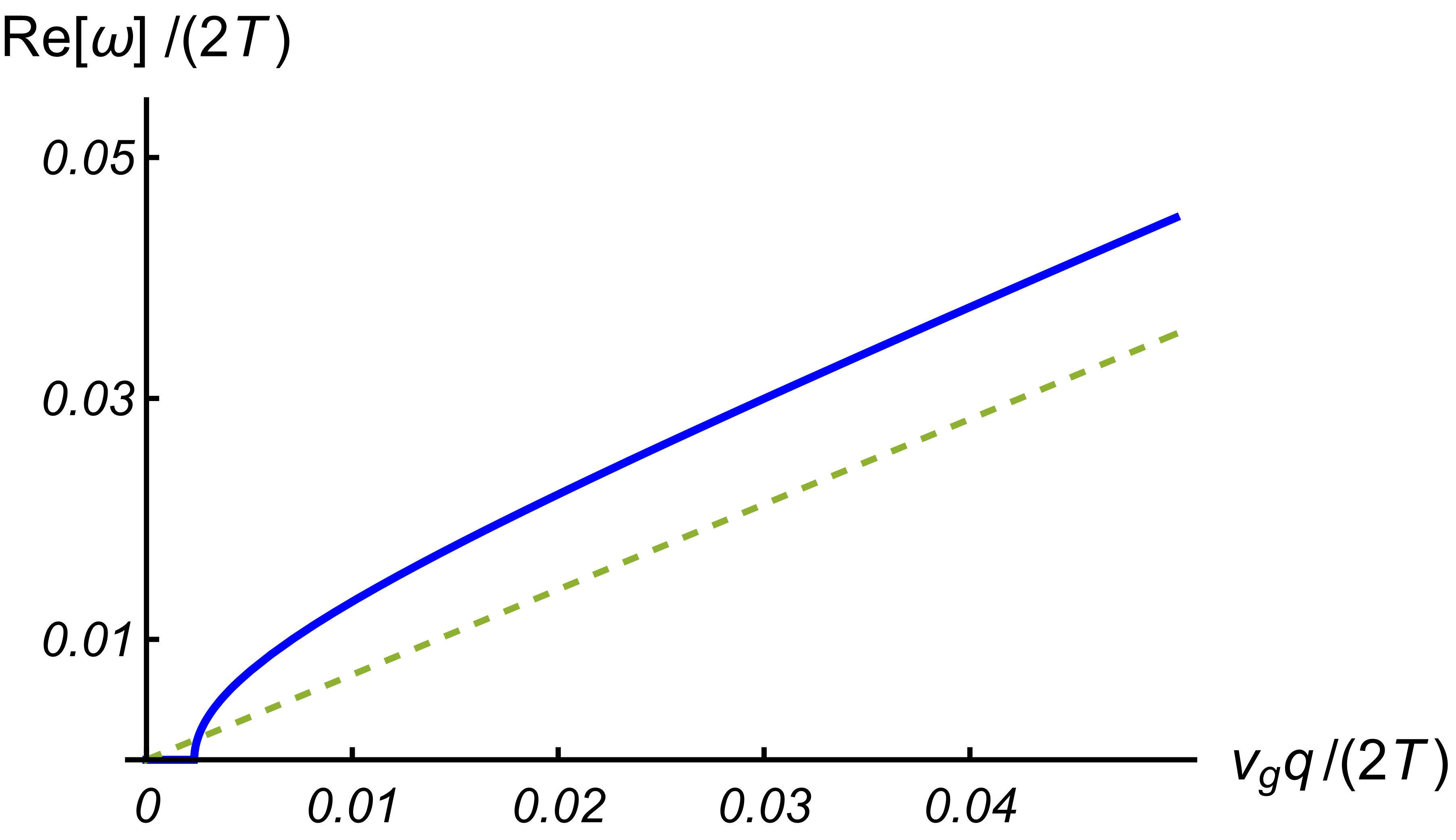
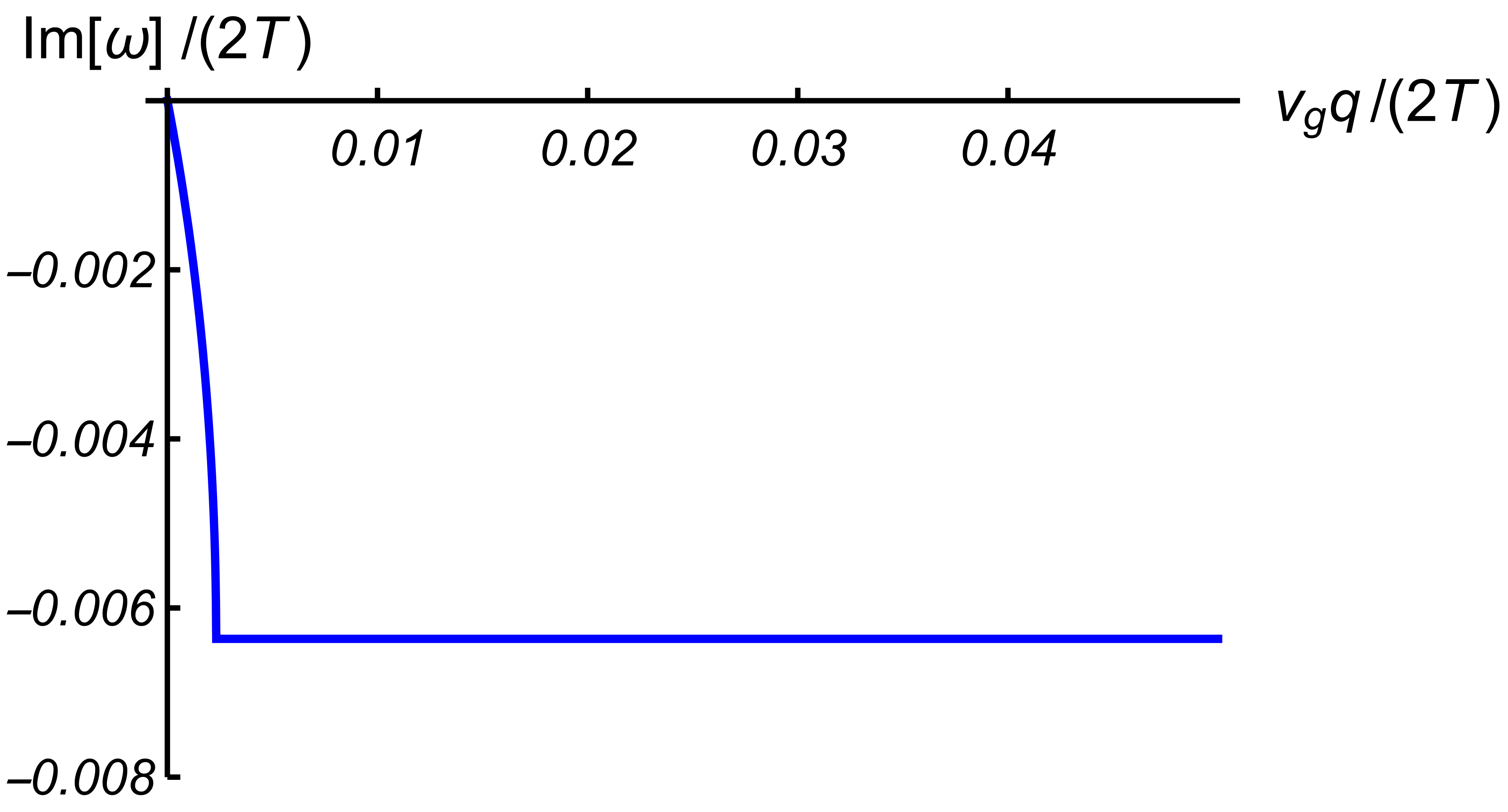
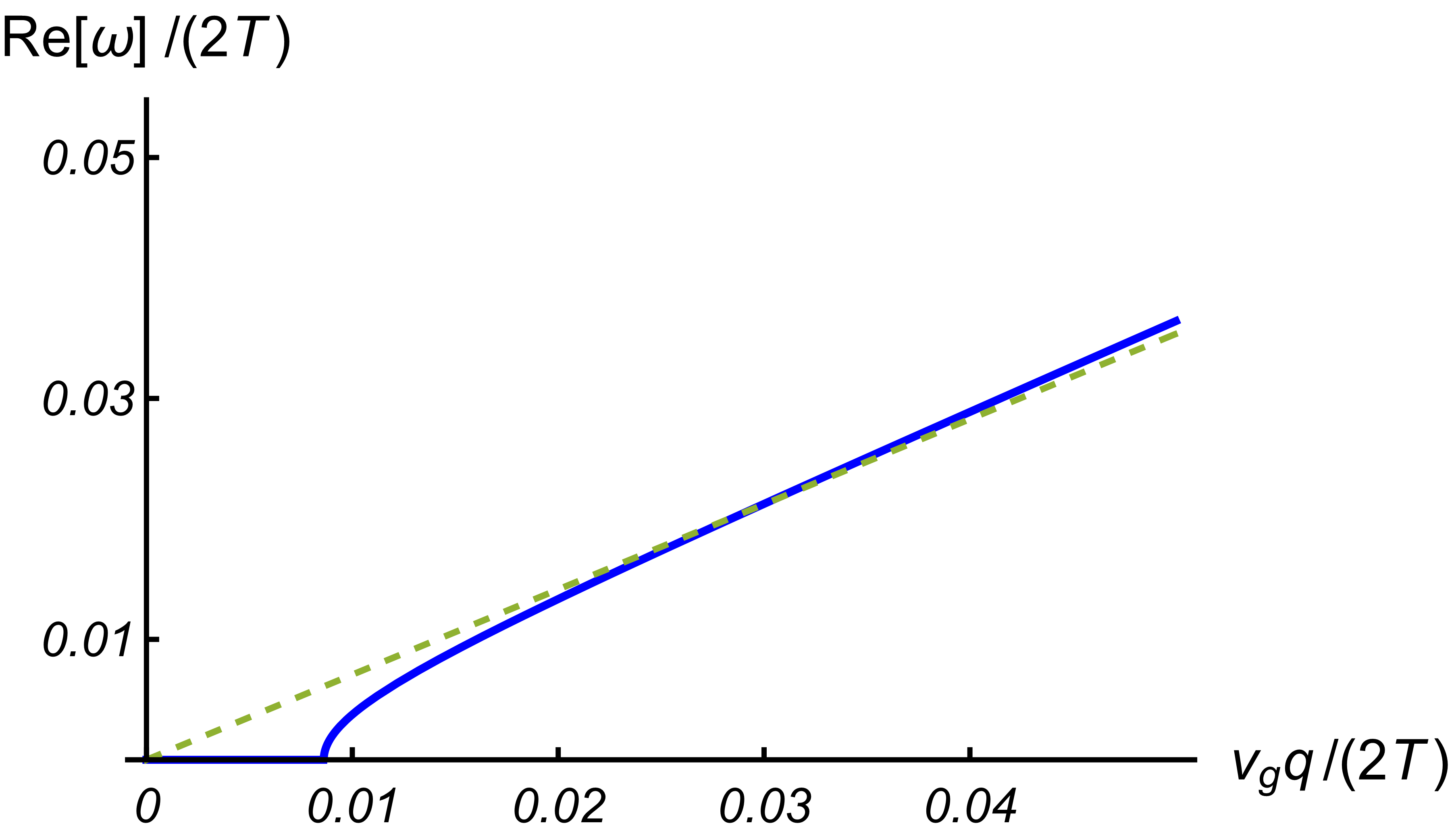
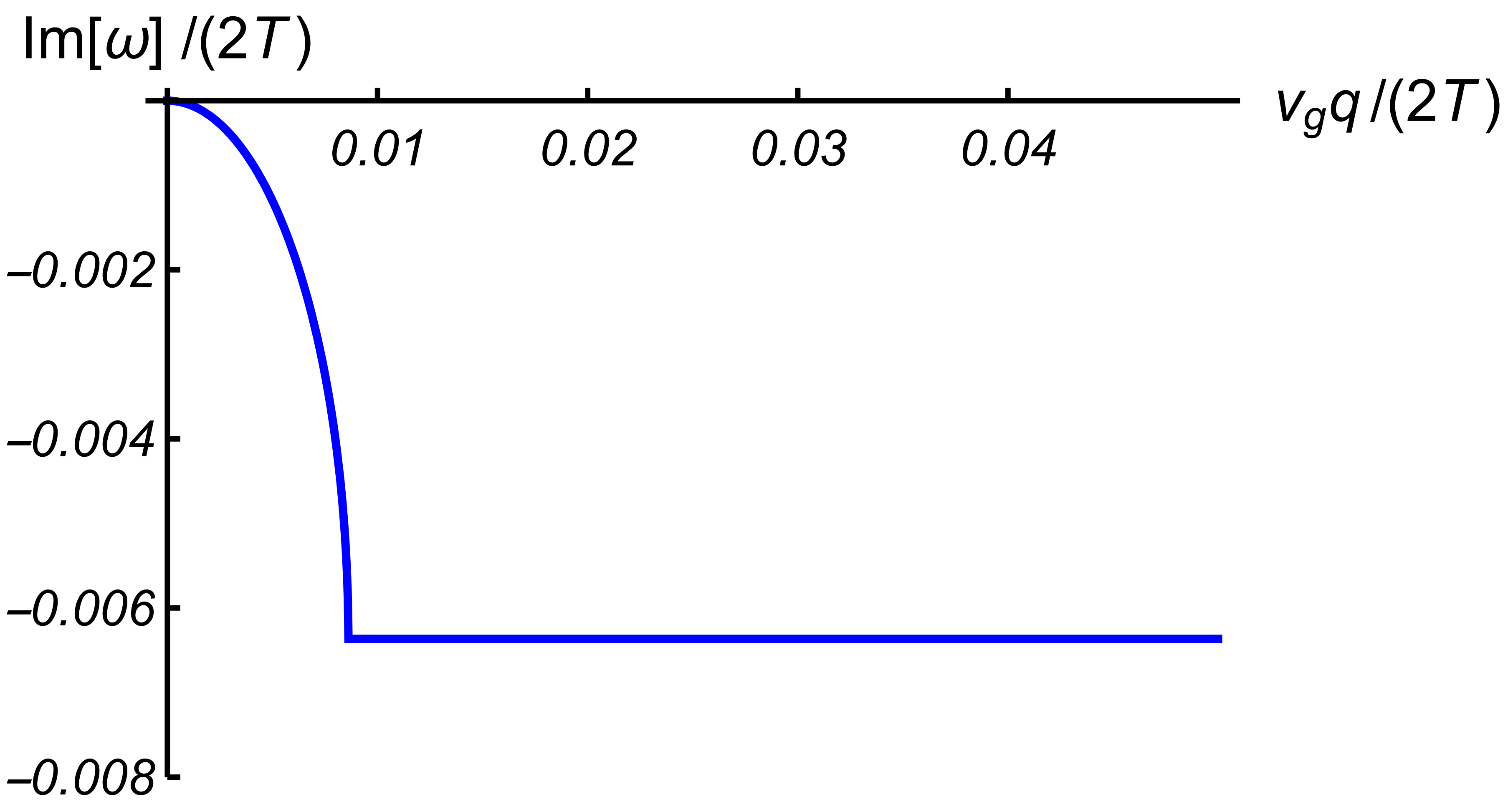
Figure 9: Real and imaginary parts of the sound dispersion in strongly doped graphene in the presence of weak disorder, but neglecting viscosity. Top panels: the result for the Coulomb screening. Bottom panels: same for a gated structure. Dashed lines represents the ideal “cosmic sound” dispersion (1).

     

     

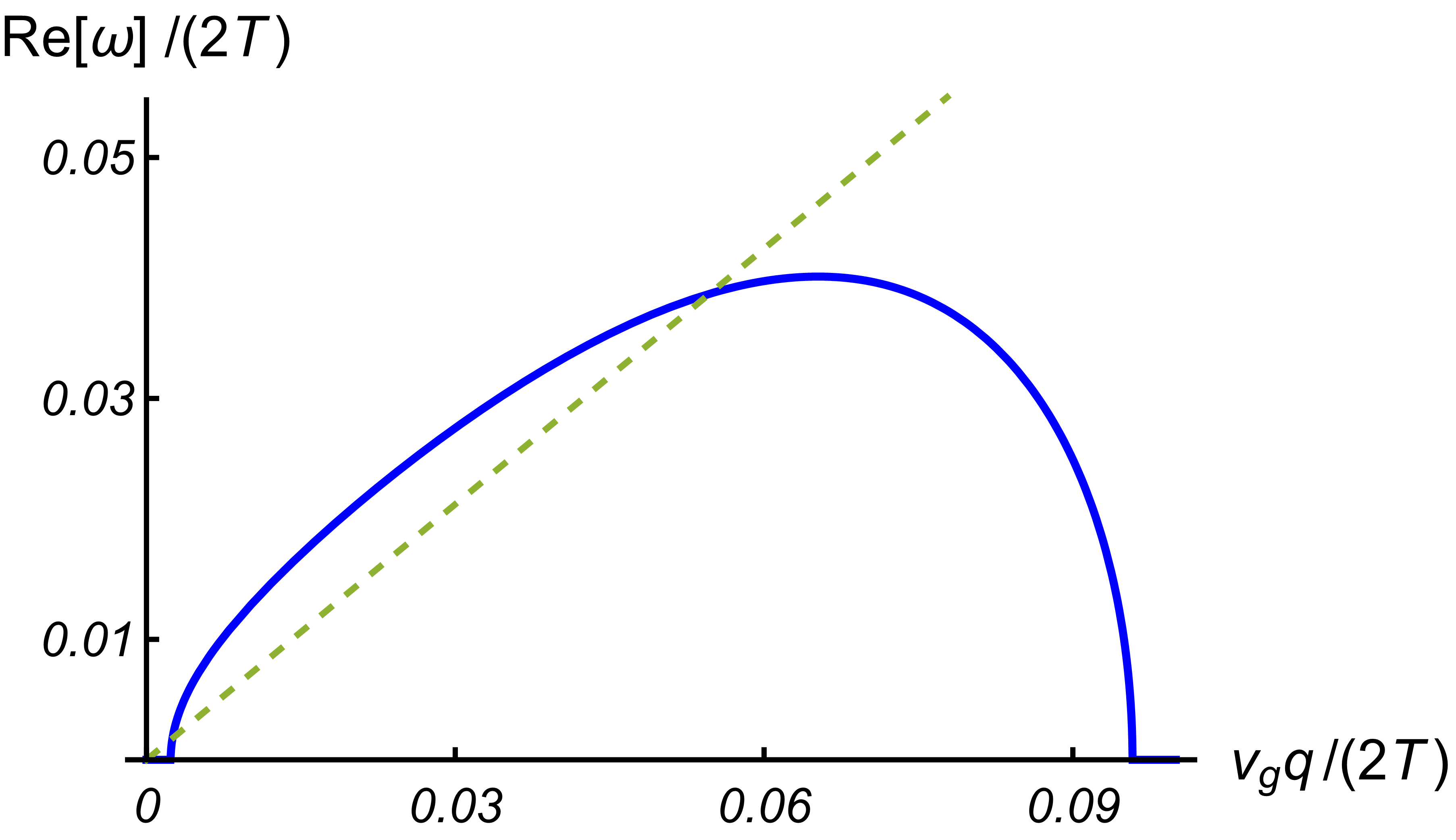
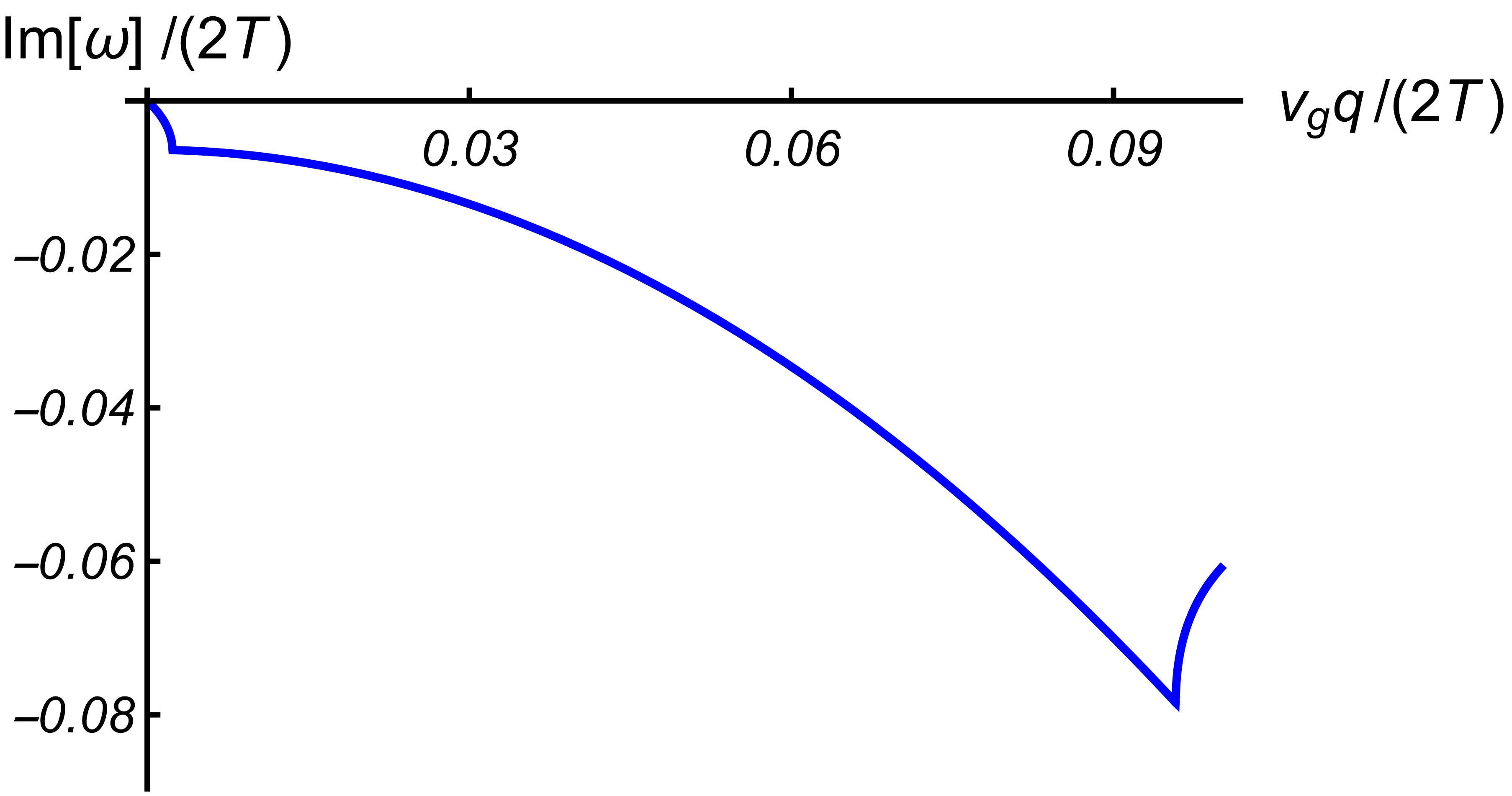
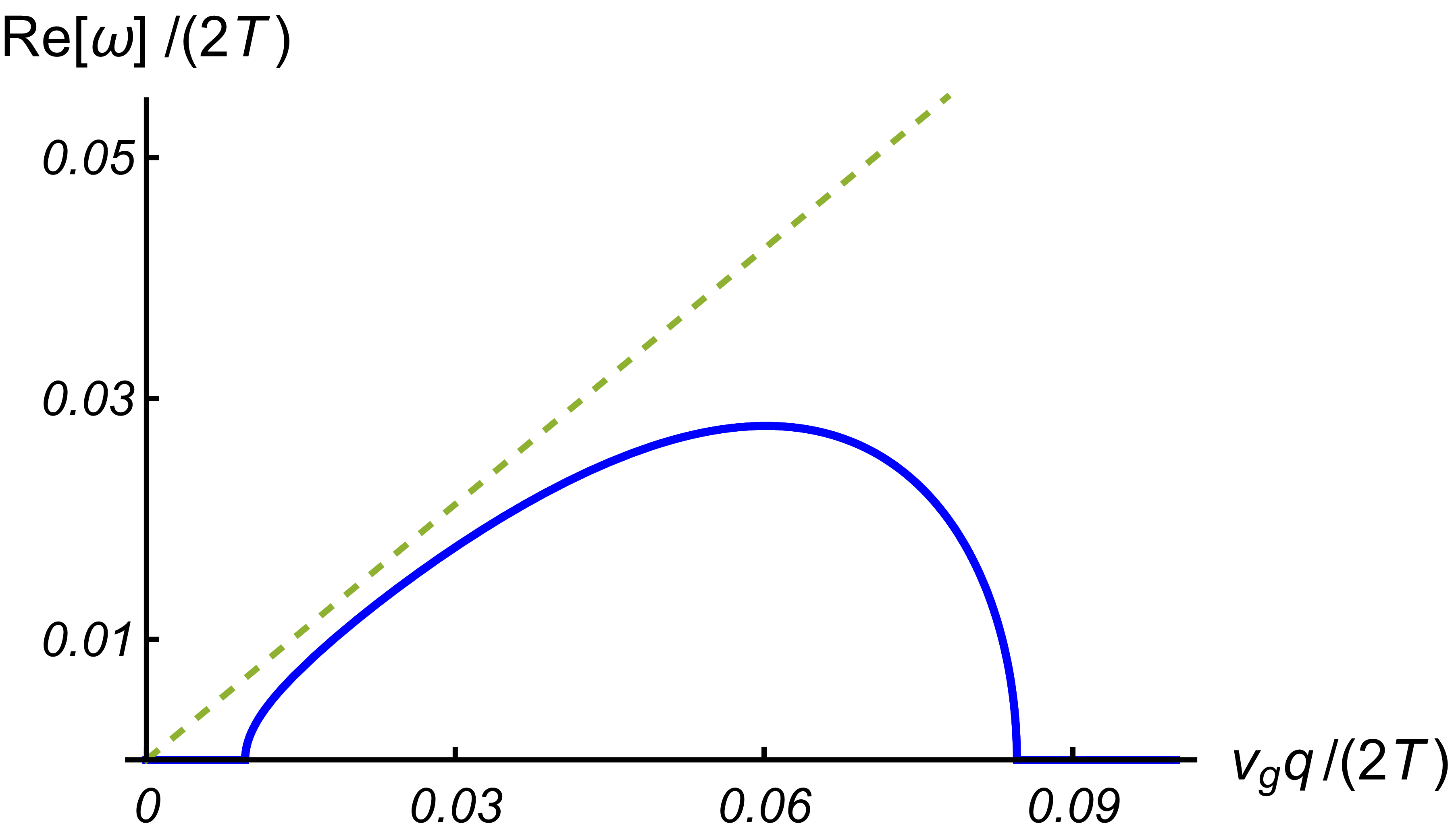
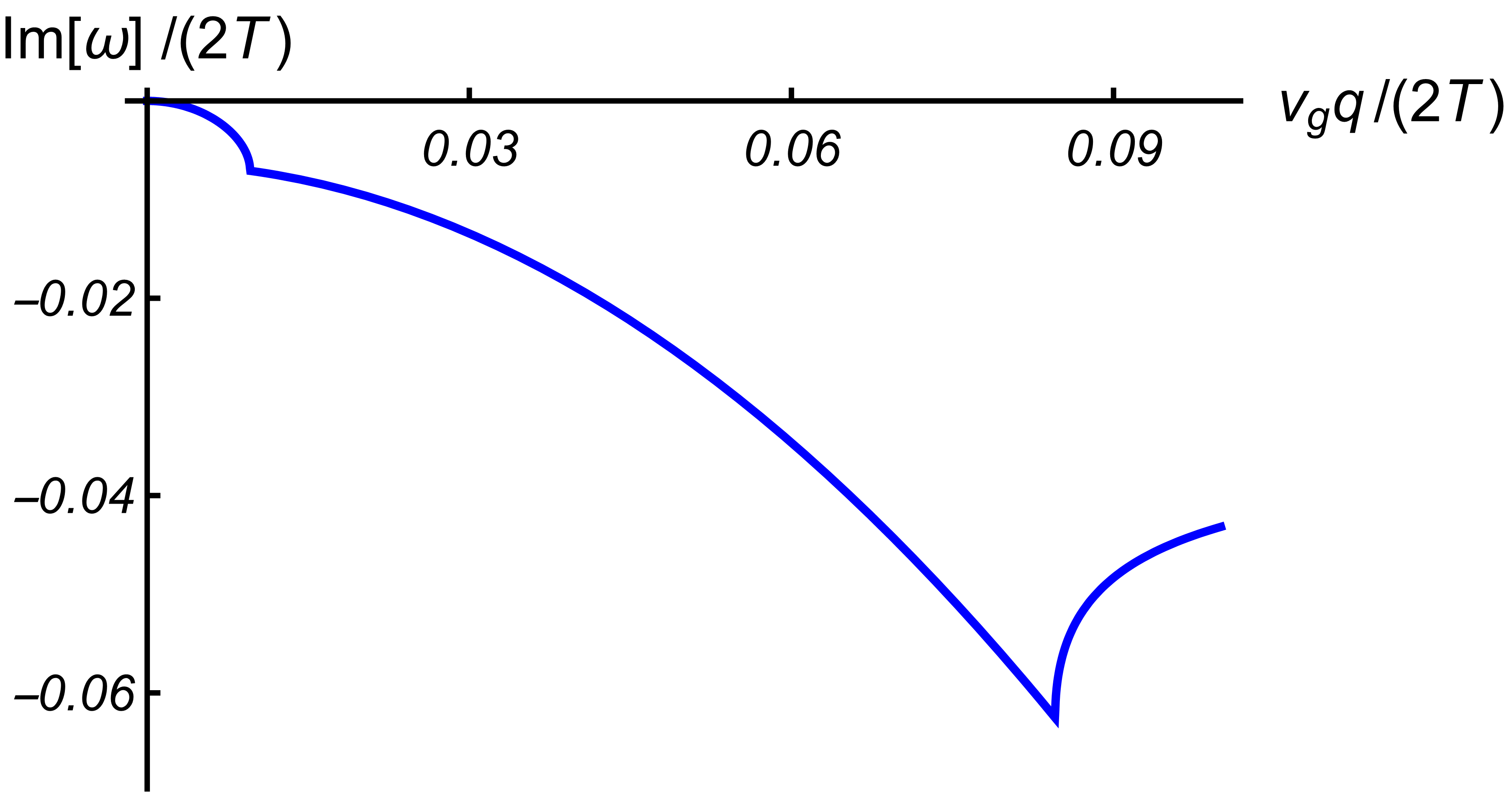
Figure 10: Real and imaginary parts and the quality factor $Q={\rm Re}\,\omega/{\rm Im}\,\omega$ of the sound dispersion in strongly doped graphene in the presence of both weak disorder and viscosity. Top panels: the result for the Coulomb screening. Bottom panels: same for a gated structure. Dashed lines represent the ideal “cosmic sound” dispersion (1).

Long-range Coulomb interaction modifies the screening contribution to the sound mode (41)

$$\omega\!=\!\sqrt{\frac{v_{g}^{2}q^{2}}{2}\!\left[1\!+\!\frac{\varkappa}{q}\right]\!-\!\frac{\left(1\!+\!\ell_{G}^{2}q^{2}\right)^{\!2}}{4\tau^{2}_{{\rm dis}}}}-\frac{i\left(1\!+\!\ell_{G}^{2}q^{2}\right)^{\!2}}{2\tau_{{\rm dis}}}\!.$$ (42)

Taking the naive limit $q\rightarrow 0$ (and $x\rightarrow\infty$) in Eq. (42), one arrives at the spectrum similar to the usual two-dimensional plasmon [15, 67]

$$\omega(q\ll\varkappa)=-\frac{i}{2\tau_{{\rm dis}}}+\sqrt{\frac{1}{2}v_{g}^{2}q\varkappa-\frac{1}{4\tau^{2}_{{\rm dis}}}}.$$ (43)

The dispersion (43) is meaningful if the following conditions are met

$$q\ell_{G}\ll 1,\quad q\ll\varkappa,\quad v_{g}^{2}\varkappa q\tau^{2}_{\rm dis}\gg 1.$$

At the same time, for the hydrodynamic approach to be valid at all, the gradients are supposed to be small on the scale that is defined by the electron-electron interaction

$$q\ell_{\rm hydro}\ll 1,\quad\ell_{\rm hydro}\sim\frac{v_{g}}{\alpha_{g}^{2}\bar{T}}.$$

These conditions to be consistent if (using the explicit form of physical quantities in the degenerate regime)

$$v_{g}\varkappa\tau_{\rm dis}\gg 1\quad\Rightarrow\quad N\alpha_{g}\mu\tau_{\rm dis}\gg 1,$$

$$\ell_{G}\ll v_{g}^{2}\varkappa\tau^{2}_{\rm dis}\quad\Rightarrow\quad N^{2}\alpha^{4}_{g}\mu\tau_{\rm dis}(\bar{T}\tau_{\rm dis})^{2}\gg 1,$$

providing a possibility to observe the dispersion (43) in a parametrically defined range of wavevectors.

The eigenvectors of the “flat zero mode” and the sound mode mix the charge, energy density, and velocity fluctuations. In that sense, the mode (43) is not a true plasmon, even though its dispersion is identical with that of the usual plasmon in two dimensions. Moreover, the dispersion (43) resembles the plasmon dispersion only in an intermediate interval of rather small $q$, while the true plasmon exists at large values of $q$.

The above dispersion can be illustrated numerically as follows. Using the same typical values $\tau_{\rm dis}^{-1}=1\,$THz, $\nu=0.2\,$m²/s (the kinematic viscosity varies only weakly with the carrier density [46]), and $T=300\,$K, as well as the typical value of the coupling constant [12, 64] $\alpha_{g}=0.23$ and the parameters characterizing the external gate in a typical graphene-on-boron nitride structure [3], the dielectric constant of the hexagonal boron nitride $\epsilon=4.4$ and the graphene to gate distance $d=80\,$nm, we plot the two dispersions (41) and (42) in Figs. 8-10. In Fig. 8, we show the two dispersions (41) and (42) in the absence of both weak disorder and viscosity. The effect of the screening can be summarized as follows. In a gated structure screening leads to a slight (for the realistic parameter values chosen above) change of slope of the sound mode dispersion. In contrast, Coulomb screening leads to a plasmon-like square-root dispersion for the smallest values of momentum, which soon turns into a linear dispersion with the same slope as the “cosmic sound” of the ideal fluid, but slightly (again, for the realistic parameter values) shifted upwards. Taking into account dissipative processes washes out qualitative differences between different types of screening. The results are also qualitatively the same for strongly doped and neutral graphene. In Fig. 9 we show the results for the dispersion in the presence of weak disorder, but still neglecting viscosity. Qualitatively, the results for both types of screening are similar with the only difference being that the real part of the dispersion in the case of the Coulomb screening is shifted upwards relative to the ideal sound dispersion, similarly to the left panel in Fig. 8, while in the case of the gated structure the resulting straight line at large enough $q$ has a slightly larger slope than $1/\sqrt{2}$.

Once viscosity is taken into account, the curves in Fig. 10 strongly resemble the results in neutral graphene, cf. Fig. 1. The results for gated graphene show only insignificant numerical differences from the curves in Fig. 1, while in the case of the Coulomb screening the real part of the dispersion appears at a smaller value of $q$ and exceeds the ideal spectrum (represented in all figures by the dotted line) in a small intermediate range of $q$.

IV Hydrodynamic collective modes and plasmons

The hydrodynamic approach is applicable in the long-time and long-wavelength limit [68, 2, 1, 45], i.e., at momenta that are small compared to the typical “equilibration” length scale $\ell_{\rm hydro}$. At higher momenta (and frequencies), the system is not in equilibrium. In this regime (sometimes referred to [27] as “collisionless”), the electronic fluid exhibits well-known collective excitations, the plasmons. In two dimensions and in the absence of impurity scattering ($\tau_{\rm{dis}}\rightarrow\infty$) the plasmon dispersion in the degenerate electron gas has the form [27]

$$\omega=\sqrt{2e^{2}\mu q}\left(1+\gamma\frac{q}{\varkappa}\right),$$ (44)

where $\gamma$ is a numerical coefficient (see below). The “proper” way to derive Eq. (44) is to evaluate the Lindhard function within the random phase approximation (RPA), which would lead [27] to the coefficient ${\gamma=3/4}$. An attempt to derive the plasmon dispersion from a macroscopic (hydrodynamic-like) theory leads to the same form (44), but with a different value for $\gamma$. This discrepancy is well known and can be attributed to the failure of the hydrodynamic description at high frequencies and momenta [27]. As a result, one concludes that the hydrodynamic collective modes have nothing to do with plasmons simply because they belong to a different parameter regime. In this Section we extend these arguments to Dirac fermions in graphene and establish the relation between the above hydrodynamic modes and plasmons.

IV.1 Degenerate regime

The case of graphene is special because of the kinematic peculiarity known as the “collinear scattering singularity” [1, 2, 15, 43, 44, 62, 19, 66, 16] leading to the existence of the two parametrically (in the weak coupling limit) different length scales associated with electron-electron interactions, ${\ell_{\rm coll}\ll\ell_{\rm hydro}}$. In an intermediate momentum range, ${\ell_{\rm{hydro}}^{-1}\ll{q}\ll\ell_{\rm coll}^{-1}}$, the hydrodynamic theory of Section I breaks down, while the linear response theory of Ref. 43 is still valid. Remarkably, the macroscopic equations of the latter theory are identical with the linearized hydrodynamic equations, so that the collective modes in the two parameter regimes coincide.

In the degenerate regime and in the absence of magnetic field, the linear response theory [43] reduces to the single macroscopic equation describing the dynamics of the electric current $\boldsymbol{J}$ (here $\rho$ is the charge density)

$$\frac{\partial\boldsymbol{J}}{\partial t}+\frac{v_{g}^{2}}{2}\boldsymbol{\nabla}\rho-\nu\Delta\boldsymbol{J}-\frac{v_{g}^{2}}{2}\frac{\partial n}{\partial\mu}e^{2}\boldsymbol{E}=-\frac{\boldsymbol{J}}{\tau_{\rm dis}},$$ (45)

which is essentially the generalized Ohm’s law. To obtain the plasmon dispersion, we introduce the Vlasov field [cf. Eq. (17)] and use the continuity equation. In the case of Coulomb interaction, the standard algebra [27] leads to the following equation

$$\omega\left(1+q^{2}\ell_{G}^{2}-i\omega\tau_{\rm dis}\right)=-iDq^{2}-i2\pi\sigma q,$$

where ${D=v_{g}^{2}\tau_{\rm dis}/2}$ and ${\sigma=v_{g}^{2}(\partial n/\partial\mu)\tau_{\rm dis}/2}$ are the diffusion coefficient and the Drude conductivity. The resulting spectrum has the form

$$\omega=\sqrt{2e^{2}\mu q\left(1\!+\!\frac{q}{\varkappa}\right)-\frac{(1\!+\!q^{2}\ell_{G}^{2})^{2}}{4\tau^{2}_{\rm dis}}}-\frac{i(1\!+\!q^{2}\ell_{G}^{2})}{2\tau_{\rm dis}}.$$ (46)

The spectrum (46) is exactly the same as Eq. (42). For a clean system (${\tau_{\rm{dis}}\rightarrow\infty}$), the expansion for small ${q\rightarrow 0}$ yields the form (44) with the “wrong” coefficient, ${\gamma=1/2}$. At the same time, the leading term (neglecting the correction for ${q\ll\varkappa}$) agrees with the standard Fermi liquid result even in the presence of disorder [67] (neglecting viscosity).

The expression (46) is valid for momenta up to $\ell_{\rm coll}^{-1}$, but in fact it becomes overdamped already at momenta of order $\ell_{\rm hydro}^{-1}$. At larger momenta, $q\gg\ell_{\rm coll}^{-1}$, the quasi-equilibrium description breaks down and the true plasmons emerge with the dispersion (44). By that time the spectrum (46) becomes purely imaginary (see Fig. 10), and hence the two modes are not connected. Similar conclusions have been reached in Ref. 24, where it was argued that Coulomb interaction precludes the appearance of hydrodynamic sound in Fermi liquids.

IV.2 Two-fluid hydrodynamics

Let us slightly digress and consider the curious case of the two-fluid hydrodynamics [69, 49, 50] in compensated semimetals. Following Ref. 49 we assume that the full electronic systems comprises two weakly coupled fluids, one consisting of electrons and another of holes. This means that the length scales $\ell_{ee}$ and $\ell_{hh}$ describing intraband electron-electron scattering are much smaller than the interband scattering length $\ell_{eh}$. In that case, the system is described by two equations similar to Eq. (45) with an extra interband scattering term

$$\frac{\partial\boldsymbol{j}_{\alpha}}{\partial t}+\frac{\langle v^{2}\rangle}{2}\boldsymbol{\nabla}n_{\alpha}-\nu\Delta\boldsymbol{j}_{\alpha}-\frac{\langle v^{2}\rangle}{2}\frac{\partial n_{\alpha}}{\partial\mu}e_{\alpha}\boldsymbol{E}=$$ (47)

$$\qquad\qquad\qquad\qquad\qquad\qquad\quad=-\frac{\boldsymbol{j}_{\alpha}}{\tau_{\rm dis}}-\frac{\boldsymbol{j}_{\alpha}-\boldsymbol{j}_{\alpha^{\prime}}}{2\tau_{eh}},$$

where $e_{h}=-e>0$, $e_{e}=e<0$, $\boldsymbol{j}_{\alpha}$ denotes the quasiparticle currents, and $\alpha^{\prime}$ denotes the other constituent. For simplicity we assume the system to be electron-hole symmetric ($\ell_{ee}=\ell_{hh}$).

Combining the two currents into the linear combinations, ${\boldsymbol{j}=\boldsymbol{j}_{e}-\boldsymbol{j}_{h}}$ and ${\boldsymbol{j}_{I}=\boldsymbol{j}_{e}+\boldsymbol{j}_{h}}$, we find the decoupled (in the absence of the magnetic field) equations

$$\frac{\partial\boldsymbol{j}}{\partial t}-\nu\Delta\boldsymbol{j}-\frac{\langle v^{2}\rangle}{2}\frac{\partial n_{I}}{\partial\mu}e\boldsymbol{E}=-\frac{\boldsymbol{j}}{\tau_{\rm dis}}-\frac{\boldsymbol{j}}{\tau_{eh}},$$ (48a)

$$\frac{\partial\boldsymbol{j}_{I}}{\partial t}+\frac{\langle v^{2}\rangle}{2}\boldsymbol{\nabla}n_{I}-\nu\Delta\boldsymbol{j}_{I}=-\frac{\boldsymbol{j}_{I}}{\tau_{\rm dis}}.$$ (48b)

Combining these equations with the two continuity equations (6b) and (6c), we find a sound-like mode

$$\omega=\sqrt{\frac{\langle v^{2}\rangle q^{2}}{2}\!-\!\left(\frac{1\!+\!q^{2}\ell_{G}^{2}}{2\tau_{\rm dis}}\!-\!\frac{1}{2\tau_{R}}\right)^{\!\!2}}-\frac{i(1\!+\!q^{2}\ell_{G}^{2})}{2\tau_{\rm dis}}-\frac{i}{2\tau_{R}},$$ (49a)

and a plasmon-like mode

$$\omega=\sqrt{\frac{\langle v^{2}\rangle\varkappa q}{2}-\frac{(1\!+\!q^{2}\ell_{G*}^{2})^{2}}{4\tau^{2}_{*}}}-\frac{i(1\!+\!q^{2}\ell_{G*}^{2})}{2\tau_{*}},$$ (49b)

where

$$\varkappa=2\pi e^{2}\frac{\partial n_{I}}{\partial\mu},\qquad\tau_{*}=\frac{\tau_{\rm dis}\tau_{eh}}{\tau_{\rm dis}\!+\!\tau_{eh}},\qquad\ell_{G*}=\sqrt{\nu\tau_{*}}.$$

In the hydrodynamic parameter range, both modes (49) are well defined. The expression under the square root in Eq. (49a) can be rewritten as

$$\frac{\langle v^{2}\rangle}{2}\left[q^{2}\left(1\!-\!\frac{\tau_{ee}}{\tau_{\rm dis}}\!+\!\frac{\tau_{ee}}{\tau_{R}}\!-\!\frac{q^{2}\ell_{ee}^{2}}{2}\right)\!-\!\frac{1}{2}\left(\frac{1}{\ell_{\rm dis}}\!-\!\frac{1}{\ell_{R}}\right)^{2}\right]\!.$$

Here ${\tau_{ee}\ll\tau_{\rm dis}}$, ${\tau_{ee}\ll\tau_{R}}$ by the assumptions of the hydrodynamic regime and ${q\ell_{ee}\ll 1}$ under the assumption of the gradient expansion in the hydrodynamic theory (here we consider a generic semimetal and hence do not have the aforementioned scale separation specific to graphene, hence we cannot extend the argument beyond the validity region of the gradient expansion). Therefore apart from the small gap due to the interplay between disorder scattering and recombination processes, the sound mode is well defined within the hydrodynamic range of momenta.

Similar arguments can be extended to the plasmon-like mode (49b). Assuming a clean system, ${\tau_{eh}\ll\tau_{\rm dis}}$, ${\tau_{*}\rightarrow\tau_{eh}}$, one finds under the square root in Eq. (49b)

$$\frac{\langle v^{2}\rangle}{2}\left[q\varkappa\!-\!q^{2}\frac{\tau_{ee}}{\tau_{eh}}\!-\!\frac{q^{4}\ell_{ee}^{2}}{2}\!-\!\frac{1}{2\ell_{eh}^{2}}\right]\!.$$

Typically, the Thomas-Fermi screening radius is smaller then the electron-electron scattering length, ${\varkappa\ell_{ee}\gg 1}$. Hence, the mode (49b) is also well defined. Here the electron-hole scattering yields the (small) gap in the dispersion similarly to the disorder scattering in Eq. (46).

IV.3 Graphene at charge neutrality

Utilizing the scale separation in graphene (see above), we can approach the question of the collective modes from the standpoint of the linear response theory of Ref. 43. Here, instead of formulating the hydrodynamic equations (6), we turn to the macroscopic equations describing the behavior of the three inequivalent currents in the system, $\boldsymbol{j}$, $\boldsymbol{j}_{I}$, and $\boldsymbol{j}_{E}$

$$\frac{\partial\boldsymbol{j}}{\partial t}+\frac{v_{g}^{2}}{2}\boldsymbol{\nabla}n-\frac{2\ln 2}{\pi}e^{2}T\boldsymbol{E}=-\frac{\boldsymbol{j}}{\tau_{\rm dis}}-\frac{\boldsymbol{j}}{\tau_{11}},$$ (50a)

$$\frac{\partial\boldsymbol{j}_{I}}{\partial t}+\frac{v_{g}^{2}}{2}\boldsymbol{\nabla}n_{I}-\frac{\gamma_{1}\nu}{T}\Delta\boldsymbol{j}_{E}=-\frac{\boldsymbol{j}_{I}}{\tau_{\rm dis}}-\frac{\boldsymbol{j}_{I}-\frac{\pi^{2}\boldsymbol{j}_{E}}{27\zeta(3)T}}{\tau_{22}\delta_{I}},$$ (50b)

$$\frac{\partial\boldsymbol{j}_{E}}{\partial t}+\frac{v_{g}^{2}}{2}\boldsymbol{\nabla}n_{E}-\nu\Delta\boldsymbol{j}_{E}=-\frac{\boldsymbol{j}_{E}}{\tau_{\rm dis}},$$ (50c)

where $\gamma_{1}$ is a numerical prefactor. At charge neutrality, the viscous term vanishes from Eq. (50a) in contrast to the two-fluid model, see Eq. (49a). In graphene, the electron and hole subsystems are strongly coupled (${\ell_{ee}=\ell_{hh}\sim\ell_{eh}}$) forming a single fluid, where the electric current is not affected by viscous effects because of electron-hole symmetry. Viscosity still affects neutral quasiparticle and energy flows in agreement with the hydrodynamic approach, where the hydrodynamic velocity in neutral graphene describes the flow of energy.

 

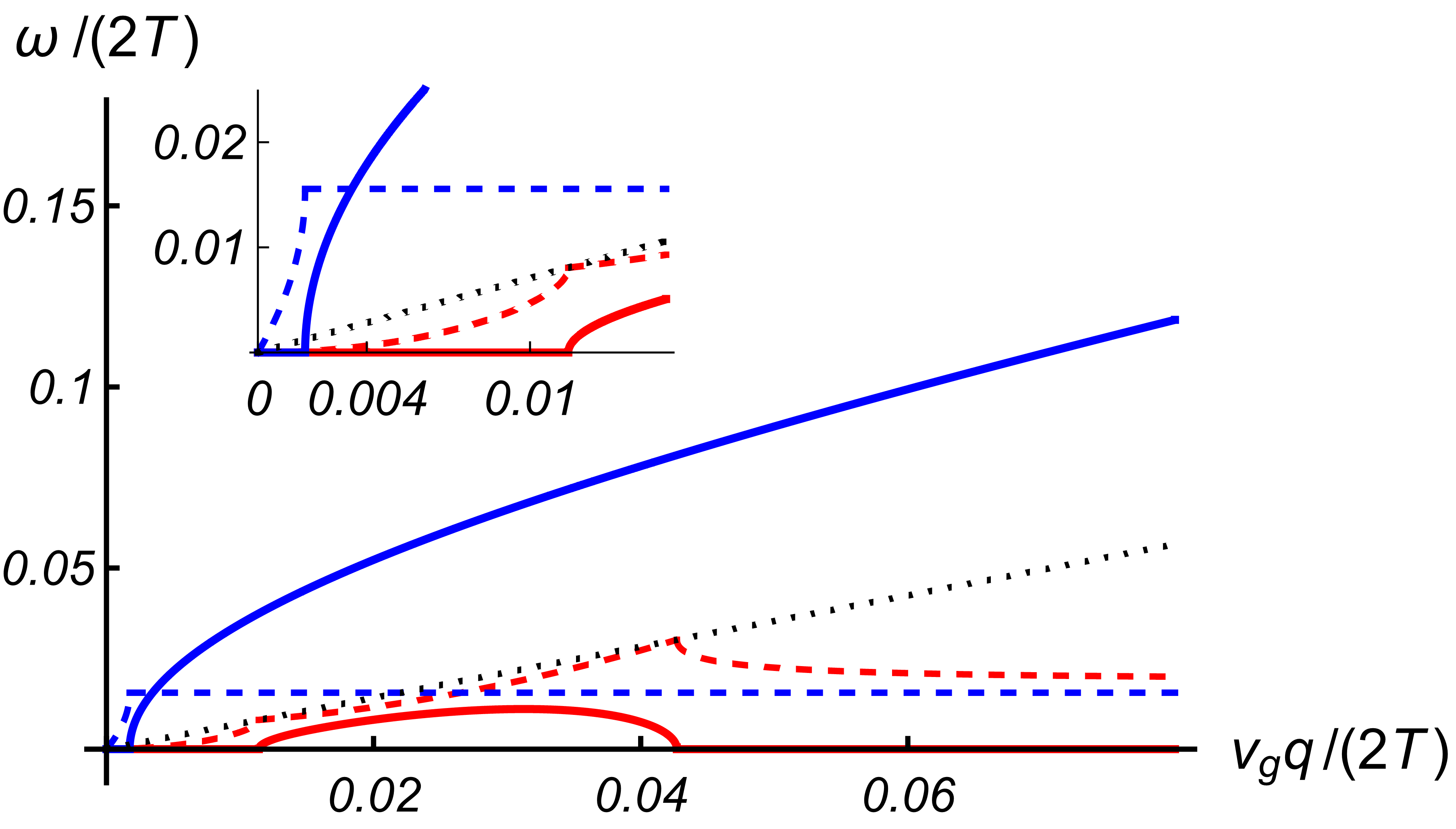
Figure 11: Comparison between the plasmon mode (54) and the sound mode (55) within the linear response theory. Solid curves show the real part of the dispersion, dashed curves the absolute value of the imaginary part. The dotted line shows the ideal “cosmic sound” dispersion (1). The plasmon dispersion is shown in blue, the sound in red. The distinction between the two modes is clearly defined by their frequencies that are much higher for the plasmon mode. Left panel shows the dispersion for a clean sample; right panel the same for the typical value $\tau_{\rm dis}^{-1}=1\,$THz. The coupling constant is taken at a model value $\alpha_{g}=0.1$, hence, no renormalization of the velocity $v_{g}$ is taken into account strongly underestimating viscosity. The real part of the sound dispersion vanishes at $\tilde{q}\approx 0.54$, which is similar to the applicability limit of the linear response theory, $\ell_{\rm coll}^{-1}$. The imaginary part exceeds the real part at a lower value of $\tilde{q}$, such that the mode becomes overdamped and disappears still within the applicability region of the theory. In the presence of disorder (right panel) the sound model is completely overdamped, see Fig. 1 for more realistic values.

Similarly to the hydrodynamic regime (Section III.0.1), the energy and charge decouple completely. Combining Eq. (50c) with the continuity equation for the energy density (18d) – that is equivalent to the linearized heat transport equation (6d) – we recover the sound mode (2).

On the other hand, combining Eq. (50a) with the continuity equation (6b) we find

$$\omega^{2}+i\omega\left(\frac{1}{\tau_{\rm dis}}+\frac{1}{\tau_{11}}\right)=\frac{v_{g}^{2}}{2}q^{2}+(4\ln 2)e^{2}Tq,$$ (51)

leading to the plasmon-like spectrum. For large enough frequencies, ${\omega\gg\tau_{11}^{-1}\gg\tau_{\rm dis}^{-1}}$, and small momenta, ${q\rightarrow 0}$, the resulting dispersion coincides with the leading behavior of the true plasmon dispersion established in Ref. 19

$$\omega=\sqrt{(4\ln 2)e^{2}Tq}\quad\Rightarrow\quad\tilde{\omega}=\sqrt{2(\ln 2)\alpha_{g}\tilde{q}},$$ (52)

where the last equality is expressed in terms of the dimensionless variables (22a), also used in Ref. 19. Note, that at large momenta, where the first term in the left-hand side of Eq. (51) dominates, the resulting dispersion resembles the cosmic sound (1), contradicting the result of Ref. 19, where the dispersion in the large-$q$ limit also becomes linear, but without the extra $\sqrt{2}$.

Considering the limit $\tau_{*}\rightarrow\infty$ in Eq. (49b), we arrive at the same result [in graphene at the charge neutrality point, ${v_{g}^{2}\varkappa/2=(4\ln 2)e^{2}T}$, while viscosity does not affect charge transport]. In the absence of disorder, the two-fluid model considered in Section IV.2 describes the electron and hole subsystems as being weakly coupled (similarly to the effect of Coulomb drag [70], but without spatial separation). Charge density fluctuations are correspond to the out-of-phase motion of electrons and holes. In the absence of the electron-hole scattering ($\tau_{*}\rightarrow\infty$), charge transport is effectively decoupled from the in-phase (imbalance) mode and hence Eq. (48a) becomes equivalent to Eq. (50a) yielding the same plasmonic mode.

Rewriting Eq. (51) in the form

$$i\omega\left[-i\omega+\frac{1}{\tau_{\rm dis}}+\frac{1}{\tau_{11}}\right]=\frac{v_{g}^{2}}{2}q^{2}+(4\ln 2)e^{2}Tq,$$

we express the plasmon dispersion in the form closely resembling Eq. (31)

$$\omega=-i\frac{\sigma(\omega)q^{2}}{e^{2}\partial n/\partial\mu}\left[1+eV_{s}(q)\frac{\partial n}{\partial\mu}\right],$$

where instead of the static conductivity (5) we find the optical conductivity [45]

$$\sigma(\omega)=\frac{2e^{2}T\ln 2}{\pi}\frac{1}{-i\omega+\tau_{11}^{-1}+\tau_{\rm dis}^{-1}}.$$

In the hydrodynamic regime ${\sigma(\omega\rightarrow 0)\rightarrow\sigma_{0}}$ and we recover the diffusive mode (31).

Resolving Eq. (51) we find the full plasmon dispersion

$$\omega=-i\frac{\tau_{\rm dis}\!+\!\tau_{11}}{2\tau_{\rm dis}\tau_{11}}\!+\!\sqrt{\frac{v_{g}^{2}}{2}q^{2}\!+\!(4\ln 2)e^{2}Tq\!-\!\frac{(\tau_{\rm dis}\!+\!\tau_{11})^{2}}{4\tau_{\rm dis}^{2}\tau_{11}^{2}}}\ .$$ (53)

To analyze the two modes – the plasmon and sound – together, we rewrite the above dispersion in dimensionless units (22a). The plasmon dispersion takes the form

$$\tilde{\omega}_{p}\!=\!\sqrt{2(\ln 2)\alpha_{g}\tilde{q}\left[1\!+\!\frac{\tilde{q}}{4(\ln 2)\alpha_{g}}\right]\!-\!\left[\frac{1}{2\tilde{\tau}_{\rm dis}}\!+\!\frac{\alpha_{g}^{2}\ln 2}{2\pi{\cal A}}\right]^{2}}$$

$$\qquad\qquad\qquad\qquad-\frac{i}{2}\!\left(\frac{1}{\tilde{\tau}_{\rm dis}}\!+\!\frac{\alpha_{g}^{2}\ln 2}{\pi{\cal A}}\right)\!,$$ (54)

where the constant ${{\cal A}\approx 0.12}$ determines the quantum conductivity at charge neutrality [52, 16, 1, 2]

$$\sigma_{Q}={\cal A}e^{2}/\alpha_{g}^{2}.$$

At the same time, the sound dispersion (1) is given by

$$\tilde{\omega}_{s}\!=\!\sqrt{\frac{\tilde{q}^{2}}{2}\!-\!\left[\frac{1}{2\tilde{\tau}_{\rm dis}}\!+\!\frac{\pi{\cal B}\tilde{q}^{2}}{9\zeta(3)\alpha_{g}^{2}}\right]^{2}}-\frac{i}{2}\!\left(\frac{1}{\tilde{\tau}_{\rm dis}}\!+\!\frac{2\pi{\cal B}\tilde{q}^{2}}{9\zeta(3)\alpha_{g}^{2}}\right)\!,$$ (55)

where the constant ${{\cal B}\approx 0.45}$ determines the shear viscosity in neutral graphene [17, 16, 1, 2]

$$\eta(\mu\!=\!0)={\cal B}T^{2}/(\alpha_{g}^{2}v_{g}^{2}).$$

In pure graphene (${\tilde{\tau}_{\rm dis}\rightarrow\infty}$) in the weak coupling limit (${\alpha_{g}\rightarrow 0}$), the regions where the two dispersions are real overlap: the plasmon dispersion (54) is real for $\tilde{q}\gg\alpha_{g}^{3}$, while the sound dispersion (55) is real for $\tilde{q}\ll\alpha_{g}^{2}$. Weak disorder does not yield any qualitative changes.

The linear response theory, Eqs. (50), is applicable at length scales larger than $\ell_{\rm coll}$, the graphene-specific scale [see Eq. (35)], reflecting the collinear scattering singularity. In dimensionless units, ${\ell_{\rm{coll}}^{-1}\sim\alpha_{g}^{2}|\ln\alpha_{g}|}$, which in the weak coupling limit greatly exceeds ${\ell_{\rm{hydro}}^{-1}\sim\alpha_{g}^{2}}$, which determines the applicability of the hydrodynamic theory of Section I. In the limit ${\tilde{\tau}_{\rm dis}\rightarrow\infty}$, the real part of the sound dispersion (55) vanishes when

$$\tilde{q}=\tilde{q}_{0}=\frac{9\zeta(3)}{\sqrt{2}\pi{\cal B}}\alpha_{g}^{2}\approx 5.41\alpha_{g}^{2}.$$

Here the large numerical coefficient may mask the difference between the two length scales $\ell_{\rm hydro}$ and $\ell_{\rm coll}$ for all but the lowest values of $\alpha_{g}$. We illustrate the resulting dispersions in Fig. 11, where we use a model value $\alpha_{g}=0.1$ to keep the two length scales well separated. Even though $\tilde{q}_{0}$ is of the same order of magnitude as $\ell_{\rm coll}$, the imaginary part of the dispersion becomes comparable to the real part at a significantly lower value of $\tilde{q}$. At that point the mode becomes overdamped and essentially disappears. Adding realistic disorder renders the mode completely overdamped, see the right panel in Fig. 11.

V Summary

In this paper we described electronic collective modes in graphene based on the hydrodynamic approach and compared the results with the more general linear response theory. Our results generalize the discussion of these issues reported in Ref. 15 within the small momentum expansion. Given the universality of hydrodynamics, the results for the collective modes in the hydrodynamic regime are applicable to other semimetals (where the momentum density represented by $\boldsymbol{u}$ is effectively decoupled from the charge transport unless the system is doped far away from charge neutrality), while the three-mode approximation used to derive the linear response theory discussed in Section IV is specific to graphene.

Our main results are illustrated in Figs. 1 and 11. The former shows the dispersion of the sound mode in the hydrodynamic regime with the viscous damping and weak disorder taken into account. Using the typical experimental values of the viscosity and disorder scattering time, we find that the sound mode in real graphene is strongly damped, making it difficult to observe the ideal “cosmic sound” dispersion (1) experimentally.

In Fig. 11 we illustrate the sound and plasmon modes in neutral graphene obtained within the linear response theory of Ref. 43 (extended beyond the stationary and uniform fields). Both modes are evaluated with the “bare” parameter values (ignoring, e.g., the renormalization of quasiparticle spectrum in graphene [46, 71]) for clarity. Effectively, this approach strongly underestimates the kinematic viscosity and hence the sound mode in Fig. 11 is much more pronounced than in Fig. 1.

The plasmon mode (54) is characterized by higher frequencies that the sound mode (55) and hence is not accessible within the standard hydrodynamic approach of Section I. The connection between the two calculations can be made by allowing for the frequency-dependent (optical) conductivity in Eqs. (25) and (31). Reducing the dissipative coefficients in the hydrodynamic theory to frequency-independent constants (following the standard approach of Ref. 18) leads to the diffusive behavior of the collective charge fluctuations, see Eq. (31). Similarly, all other hydrodynamic collective modes (except for the sound mode) are characterized by purely imaginary spectra. This should be contrasted with the linear response theory, Eqs. (50), that allows for the frequency-dependent conductivities leading to the real plasmon dispersion (54), as well as a third (neutral) collective mode following from Eqs. (50b) and (6c). The fact that these additional (to the sound) modes can be reached within the linear response theory and connected to the hydrodynamic description should be attributed to the scale separation in graphene (due to the kinematic peculiarity of Dirac fermions [62, 44, 1, 2, 16]), see Eq. (35). All other qualitative conclusions of the paper are valid in a wider class of semimetals. The obtained collective modes can be observed using the by now standard plasmonics experiments, see Refs. 32, 33, 34, 30, 31, 35, 36, 37, 38.

References

Narozhny et al. [2017]
B. N. Narozhny,
I. V. Gornyi,
A. D. Mirlin,
and
J. Schmalian,
Annalen der Physik 529,
1700043 (2017).
Lucas and Fong [2018]
A. Lucas and
K. C. Fong,
J. Phys: Condens. Matter 30,
053001 (2018).
Bandurin et al. [2016]
D. A. Bandurin,
I. Torre,
R. Krishna Kumar,
M. Ben Shalom,
A. Tomadin,
A. Principi,
G. H. Auton,
E. Khestanova,
K. S. Novoselov,
I. V. Grigorieva,
et al., Science
351, 1055 (2016).
Crossno et al. [2016]
J. Crossno,
J. K. Shi,
K. Wang,
X. Liu,
A. Harzheim,
A. Lucas,
S. Sachdev,
P. Kim,
T. Taniguchi,
K. Watanabe,
et al., Science
351, 1058 (2016).
Moll et al. [2016]
P. J. W. Moll,
P. Kushwaha,
N. Nandi,
B. Schmidt, and
A. P. Mackenzie,
Science 351,
1061 (2016).
Krishna Kumar et al. [2017]
R. Krishna Kumar,
D. A. Bandurin,
F. M. D. Pellegrino,
Y. Cao,
A. Principi,
H. Guo,
G. H. Auton,
M. Ben Shalom,
L. A. Ponomarenko,
G. Falkovich,
et al., Nat. Phys.
13, 1182 (2017).
Ghahari et al. [2016]
F. Ghahari,
H.-Y. Xie,
T. Taniguchi,
K. Watanabe,
M. S. Foster,
and P. Kim,
Phys. Rev. Lett. 116,
136802 (2016).
Bandurin et al. [2018]
D. A. Bandurin,
A. V. Shytov,
L. S. Levitov,
R. Krishna Kumar,
A. I. Berdyugin,
M. Ben Shalom,
I. V. Grigorieva,
A. K. Geim, and
G. Falkovich,
Nat. Commun. 9,
4533 (2018).
Berdyugin et al. [2019]
A. I. Berdyugin,
S. G. Xu,
F. M. D. Pellegrino,
R. Krishna Kumar,
A. Principi,
I. Torre,
M. B. Shalom,
T. Taniguchi,
K. Watanabe,
I. V. Grigorieva,
et al., Science
364, 162 (2019).
Braem et al. [2018]
B. A. Braem,
F. M. D. Pellegrino,
A. Principi,
M. Röösli,
C. Gold,
S. Hennel,
J. V. Koski,
M. Berl,
W. Dietsche,
W. Wegscheider,
et al., Phys. Rev. B
98, 241304(R)
(2018).
Jaoui et al. [2018]
A. Jaoui,
B. Fauqué,
C. W. Rischau,
A. Subedi,
C. Fu,
J. Gooth,
N. Kumar,
V. Süß,
D. L. Maslov,
C. Felser,
et al., npj Quantum Materials
3, 64 (2018).
Gallagher et al. [2019]
P. Gallagher,
C.-S. Yang,
T. Lyu,
F. Tian,
R. Kou,
H. Zhang,
K. Watanabe,
T. Taniguchi,
and F. Wang,
Science 364,
158 (2019).
Ku et al. [2020]
M. J. H. Ku,
T. X. Zhou,
Q. Li,
Y. J. Shin,
J. K. Shi,
C. Burch,
L. E. Anderson,
A. T. Pierce,
Y. Xie,
A. Hamo, et al.,
Nature 583,
537 (2020).
Sulpizio et al. [2019]
J. A. Sulpizio,
L. Ella,
A. Rozen,
J. Birkbeck,
D. J. Perello,
D. Dutta,
M. Ben-Shalom,
T. Taniguchi,
K. Watanabe,
T. Holder,
et al., Nature
576, 75 (2019).
Briskot et al. [2015]
U. Briskot,
M. Schütt,
I. V. Gornyi,
M. Titov,
B. N. Narozhny,
and A. D.
Mirlin, Phys. Rev. B
92, 115426
(2015).
Narozhny [2019a]
B. N. Narozhny,
Annals of Physics 411,
167979 (2019a).
Müller et al. [2009]
M. Müller,
J. Schmalian,
and L. Fritz,
Phys. Rev. Lett. 103,
025301 (2009).
Landau and Lifshitz [1959]
L. D. Landau and
E. M. Lifshitz,
Fluid Mechanics (Pergamon Press,
London, 1959).
Schütt et al. [2011]
M. Schütt,
P. M. Ostrovsky,
I. V. Gornyi,
and A. D.
Mirlin, Phys. Rev. B
83, 155441
(2011).
Phan et al. [2013]
T. V. Phan,
J. C. W. Song,
and L. S.
Levitov (2013), eprint arXiv:1306.4972.
Levitov et al. [2013]
L. S. Levitov,
A. V. Shtyk, and
M. V. Feigelman,
Phys. Rev. B 88,
235403 (2013).
Sun et al. [2018]
Z. Sun,
D. N. Basov, and
M. M. Fogler,
Proceedings of the National Academy of Sciences
115, 3285 (2018).
Svintsov [2018]
D. Svintsov,
Phys. Rev. B 97,
121405(R) (2018).
Lucas and Das Sarma [2018]
A. Lucas and
S. Das Sarma,
Phys. Rev. B 97,
115449 (2018).
Kiselev and Schmalian [2020]
E. I. Kiselev and
J. Schmalian,
Phys. Rev. B 102,
245434 (2020).
Fateev and Popov [2020]
D. V. Fateev and
V. V. Popov,
Semiconductors 54,
941 (2020).
Giuliani and Vignale [2005]
G. Giuliani and
G. Vignale,
Quantum Theory of the Electron Liquid
(Cambridge University Press, 2005).
Hill et al. [2009]
A. Hill,
S. A. Mikhailov,
and K. Ziegler,
EPL (Europhysics Letters) 87,
27005 (2009).
Principi et al. [2011]
A. Principi,
R. Asgari, and
M. Polini,
Solid State Communications 151,
1627 (2011).
Fei et al. [2012]
Z. Fei,
A. S. Rodin,
G. O. Andreev,
W. Bao,
A. S. McLeod,
M. Wagner,
L. M. Zhang,
Z. Zhao,
M. Thiemens,
G. Dominguez,
et al., Nature
487, 82 (2012).
Chen et al. [2012]
J. Chen,
M. Badioli,
P. Alonso-González,
S. Thongrattanasiri,
F. Huth,
J. Osmond,
M. Spasenović,
A. Centeno,
A. Pesquera,
P. Godignon,
et al., Nature
487, 77 (2012).
Ni et al. [2016]
G. X. Ni,
L. Wang,
M. D. Goldflam,
M. Wagner,
Z. Fei,
A. S. McLeod,
M. K. Liu,
F. Keilmann,
B. Özyilmaz,
A. H. Castro Neto,
et al., Nature Photonics
10, 244 (2016).
Lundeberg et al. [2017]
M. B. Lundeberg,
Y. Gao,
R. Asgari,
C. Tan,
B. Van Duppen,
M. Autore,
P. Alonso-González,
A. Woessner,
K. Watanabe,
T. Taniguchi,
et al., Science
357, 187 (2017).
Alcaraz Iranzo
et al. [2018]
D. Alcaraz Iranzo,
S. Nanot,
E. J. C. Dias,
I. Epstein,
C. Peng,
D. K. Efetov,
M. B. Lundeberg,
R. Parret,
J. Osmond,
J.-Y. Hong,
et al., Science
360, 291 (2018).
Novelli et al. [2020]
P. Novelli,
I. Torre,
F. H. L. Koppens,
F. Taddei, and
M. Polini,
Phys. Rev. B 102,
125403 (2020).
Giovannini et al. [2020]
T. Giovannini,
L. Bonatti,
M. Polini, and
C. Cappelli,
The Journal of Physical Chemistry Letters
11, 7595 (2020).
Hesp et al. [2019]
N. C. H. Hesp,
I. Torre,
D. Rodan-Legrain,
P. Novelli,
Y. Cao,
S. Carr,
S. Fang,
P. Stepanov,
D. Barcons-Ruiz,
H. Herzig-Sheinfux,
et al. (2019), eprint arXiv:1910.07893.
Costa et al. [2021]
A. T. Costa,
P. A. D. Gonçalves,
D. N. Basov,
F. H. L. Koppens,
N. A. Mortensen,
and N. M. R.
Peres, PNAS 118,
e2012847118 (2021).
Klein et al. [2019]
A. Klein,
D. L. Maslov,
L. P. Pitaevskii,
and A. V.
Chubukov, Phys. Rev. Research
1, 033134 (2019).
Ferreira et al. [2020]
B. A. Ferreira,
B. Amorim,
A. J. Chaves,
and N. M. R.
Peres, Phys. Rev. A
101, 033817
(2020).
Klein et al. [2020]
A. Klein,
D. L. Maslov,
and A. V.
Chubukov, npj Quantum Mater.
5, 55 (2020).
Raines et al. [2021]
Z. M. Raines,
V. I. Fal’ko,
and L. I.
Glazman, Phys. Rev. B
103, 075422
(2021).
Narozhny et al. [2015]
B. N. Narozhny,
I. V. Gornyi,
M. Titov,
M. Schütt,
and A. D.
Mirlin, Phys. Rev. B
91, 035414
(2015).
Fritz et al. [2008]
L. Fritz,
J. Schmalian,
M. Müller, and
S. Sachdev,
Phys. Rev. B 78,
085416 (2008).
Narozhny [2019b]
B. N. Narozhny,
Phys. Rev. B 100,
115434 (2019b).
Narozhny and Schütt [2019]
B. N. Narozhny and
M. Schütt,
Phys. Rev. B 100,
035125 (2019).
Scaffidi et al. [2017]
T. Scaffidi,
N. Nandi,
B. Schmidt,
A. P. Mackenzie,
and J. E. Moore,
Phys. Rev. Lett. 118,
226601 (2017).
Pellegrino et al. [2017]
F. M. D. Pellegrino,
I. Torre, and
M. Polini,
Phys. Rev. B 96,
195401 (2017).
Alekseev
et al. [2018a]
P. S. Alekseev,
A. P. Dmitriev,
I. V. Gornyi,
V. Y. Kachorovskii,
B. N. Narozhny,
and M. Titov,
Phys. Rev. B 97,
085109 (2018a).
Alekseev
et al. [2018b]
P. S. Alekseev,
A. P. Dmitriev,
I. V. Gornyi,
V. Y. Kachorovskii,
B. N. Narozhny,
and M. Titov,
Phys. Rev. B 98,
125111 (2018b).
Danz and Narozhny [2020]
S. Danz and
B. N. Narozhny,
2D Materials 7,
035001 (2020).
Kashuba [2008]
A. B. Kashuba,
Phys. Rev. B 78,
085415 (2008).
Foster and Aleiner [2009]
M. S. Foster and
I. L. Aleiner,
Phys. Rev. B 79,
085415 (2009).
Xie and Levchenko [2019]
H.-Y. Xie and
A. Levchenko,
Phys. Rev. B 99,
045434 (2019).
Narozhny and Gornyi [2021]
B. N. Narozhny and
I. V. Gornyi
(2021), eprint arXiv:2102.00207.
Kashuba et al. [2018]
O. Kashuba,
B. Trauzettel,
and L. W.
Molenkamp, Phys. Rev. B
97, 205129
(2018).
Song et al. [2012]
J. C. W. Song,
M. Y. Reizer,
and L. S.
Levitov, Phys. Rev. Lett.
109, 106602
(2012).
Titov et al. [2013]
M. Titov,
R. V. Gorbachev,
B. N. Narozhny,
T. Tudorovskiy,
M. Schütt,
P. M. Ostrovsky,
I. V. Gornyi,
A. D. Mirlin,
M. I. Katsnelson,
K. S. Novoselov,
et al., Phys. Rev. Lett.
111, 166601
(2013).
Vasileva et al. [2016]
G. Y. Vasileva,
D. Smirnov,
Y. L. Ivanov,
Y. B. Vasilyev,
P. S. Alekseev,
A. P. Dmitriev,
I. V. Gornyi,
V. Y. Kachorovskii,
M. Titov,
B. N. Narozhny,
et al., Phys. Rev. B
93, 195430
(2016).
Alekseev et al. [2015]
P. S. Alekseev,
A. P. Dmitriev,
I. V. Gornyi,
V. Y. Kachorovskii,
B. N. Narozhny,
M. Schütt, and
M. Titov,
Phys. Rev. Lett. 114,
156601 (2015).
Aleiner and Shklovskii [1994]
I. L. Aleiner and
B. I. Shklovskii,
Phys. Rev. B 49,
13721 (1994).
Müller et al. [2008]
M. Müller,
L. Fritz, and
S. Sachdev,
Phys. Rev. B 78,
115406 (2008).
Li et al. [2020]
S. Li,
A. Levchenko,
and A. V.
Andreev, Phys. Rev. B
102, 075305
(2020).
Kozikov et al. [2010]
A. A. Kozikov,
A. K. Savchenko,
B. N. Narozhny,
and A. V.
Shytov, Phys. Rev. B
82, 075424
(2010).
Das Sarma et al. [2011]
S. Das Sarma,
S. Adam,
E. H. Hwang, and
E. Rossi,
Rev. Mod. Phys. 83,
407 (2011).
Schütt et al. [2013]
M. Schütt,
P. M. Ostrovsky,
M. Titov,
I. V. Gornyi,
B. N. Narozhny,
and A. D.
Mirlin, Phys. Rev. Lett.
110, 026601
(2013).
Zala et al. [2001]
G. Zala,
B. N. Narozhny,
and I. L.
Aleiner, Phys. Rev. B
64, 214204
(2001).
Lifshitz and Pitaevskii [1981]
E. M. Lifshitz and
L. P. Pitaevskii,
Physical Kinetics (Pergamon
Press, London, 1981).
Alekseev et al. [2017]
P. S. Alekseev,
A. P. Dmitriev,
I. V. Gornyi,
V. Y. Kachorovskii,
B. N. Narozhny,
M. Schütt, and
M. Titov,
Phys. Rev. B 95,
165410 (2017).
Narozhny and Levchenko [2016]
B. N. Narozhny and
A. Levchenko,
Rev. Mod. Phys. 88,
025003 (2016).
Sheehy and Schmalian [2007]
D. E. Sheehy and
J. Schmalian,
Phys. Rev. Lett. 99,
226803 (2007).