Short-Term Memory Optimization in Recurrent Neural Networks by Autoencoder-based Initialization
Abstract
Training RNNs to learn long-term dependencies is difficult due to vanishing gradients. We explore an alternative solution based on explicit memorization using linear autoencoders for sequences, which allows to maximize the short-term memory and that can be solved with a closed-form solution without backpropagation. We introduce an initialization schema that pretrains the weights of a recurrent neural network to approximate the linear autoencoder of the input sequences and we show how such pretraining can better support solving hard classification tasks with long sequences. We test our approach on sequential and permuted MNIST. We show that the proposed approach achieves a much lower reconstruction error for long sequences and a better gradient propagation during the finetuning phase.
1 Introduction
Recurrent neural networks are difficult to train due to vanishing gradient problems Hochreiter (1998); Bengio et al. (1994) that limit the ability to learn long-term dependencies. Theoretically, long-term dependencies can be easily learned by starting from an hidden state representation that encodes the entire sequence, giving immediate access to the past history through the hidden state vector. Learning such a representation requires maximizing the short-term memory (STM) capacity of the RNN Jaeger and Haas (2004). Unfortunately, this objective is hard to optimize by backpropagation (BP) due to the vanishing gradient problem.
In this paper, we address the problem of maximizing the STM by avoiding BP using linear autoencoders, which can be easily optimized with a closed-form solution Pasa and Sperduti (2014). We exploit linear autoencoders as a means to initialize RNNs to approximate the linear autoencoder for the input sequences. To reduce the approximation error of such an initialization, caused by the RNN nonlinearity, we propose to use a linear recurrence, removing the nonlinearity in the recurrent update. We show how a recently proposed RNN architecture, the Linear Memory Network (LMN) Carta et al. (2020a); Bacciu et al. (2019), can be exploited to this end by combining linear and nonlinear units without reducing the expressiveness of the model. We test our approach on a classic benchmark for RNNs, showing that it is competitive with state-of-the-art architectures. Furthermore, we show that the proposed autoencoder initialization maximizes the STM compared to a random initialization.
2 Optimizing the Short-Term Memory
In this section, we show how to optimize the short-term memory without BP. The STM capacity measures the ability of a recurrent model to remember and reconstruct past elements of the input sequence Jaeger and Haas (2004). We build on a recurrent encoder model , and a corresponding decoder , which may be a feedforward model trained to reconstruct or a recurrent model applied for timesteps. We measure the STM with the reconstruction error . We can maximize the STM of the encoder by minimizing . This objective facilitates learning longer dependencies by allowing to directly reconstruct past elements. Unfortunately, optimizing the STM by BP is difficult due to the vanishing gradient. Furthermore, autoencoding requires to reconstruct the entire input, which means that the maximum dependency length depends on the maximum length of the input sequences. See the additional material (Appendix B) for an example of MNIST images reconstruction with different recurrent models. The reconstructions clearly show that models trained by backpropagation fail to solve autoencoding problems.
A linear autoencoder for sequences (LAES) Sperduti (2006, 2007) is a linear recurrent model composed of a linear dynamical system (encoder) and a linear decoder. The autoencoder takes as input a sequence of vectors and computes an internal state vector as follows:
where matrices and are the encoder parameters, is the decoding matrix and and are the reconstructions of the current input and the previous memory state. Pasa and Sperduti (2014) provide a closed-form solution for the optimal linear autoencoder. The corresponding decoder parameters can be reconstructed from the encoder as .
3 Linear Memory Network
Using the LAES introduced in Section 2, we can maximize the STM capacity of recurrent neural networks while avoiding the BP through time. However, such a model is limited to a linear encoding of the sequence. Recurrent neural networks have nonlinear recurrent updates that cannot be used to model a LAES. To solve this issue, the Linear Memory Network (LMN) Bacciu et al. (2019) combines a LAES within a nonlinear recurrent architecture. The LMN computes a hidden state and a separate memory state . The hidden state is computed with a nonlinear transformation of the input and previous memory state, while the memory is updated with a linear recurrence using the current hidden state and the previous memory as follows:
where are the model parameters and is a non-linear activation function ( in our experiments).
Notice that the linearity of the memory update function does not limit the model’s expressiveness. In fact, given an RNN with parameters and such that , we can define an equivalent LMN such that by setting the parameters as .
4 Initialization with a Linear Autoencoder for Sequences
We can use the LAES to initialize recurrent models to encode the input sequences into a minimal hidden state, increasing their short-term memory compared to random initializations. We define a linear recurrent model which uses the autoencoder to encode the input sequences within a single vector, i.e. the memory state of the autoencoder. To predict the desired target, we can train a linear readout that takes as input the states of the autoencoder as follows:
| (1) | |||
| (2) |
where and are the parameters of the autoencoder trained to reconstruct the input sequences and are the parameters of a linear model trained to predict the target output from . Figure 1(a) shows a schematic view of the architecture.
Pasa and Sperduti (2014) propose to initialize an RNN with the linear RNN defined in Eq. 1 and 2 as:
Notice that the initialization above is an approximation of the original LAES due to the presence of the nonlinear activation function. The quality of such an approximation depends on the values of the hidden activations . For small values close to zero, the activation function is approximately linear, and therefore the approximation error is negligible. However, larger hidden activation values saturate the function, incuring in large approximation errors. In practice, we find that the correspondence between the linear autoencoder and the initialized RNN degrades quickly due to the accumulation of errors through time. To solve this problem, we put forward the use of a LMN, which provides a linear recurrence, in place of the RNN above. The LMN model is initialized as follows:
where the parameters are , , . Such an initialization is an approximation of the linear RNN, but since the nonlinearity only affects the input transformation and not the recurrence, the approximation is closer to the original linear RNN. In practice, we did not find any difference between the linear RNN and LMN accuracy after the initialization. Figures 1(b) and 1(c) show a schematic view of the architectures.
5 Experiments
We evaluate the performance of the autoencoder initialization and its effect on gradient propagation. Furthermore, we want to verify if finetuning of the recurrent units by BP is necessary. We compare the following models, along with baselines from the literature, the RNN and LMN, both with orthogonal or LAES initialization:
- LAES-Linear
-
A LAES with a linear classifier trained by pseudoinverse. The model does not use BP.
- LAES-SVM
-
A LAES with an SVM classifier. The model does not use BP.
- LAES-FF
-
A LAES with a feedforward classifier. The model uses truncated BP, propagating the gradient only through the feedforward units, leaving the recurrent connections fixed.
Please check the additional material for details about the chosen baselines and the experimental setup. We test the proposed model on sequential and permuted MNIST Le et al. (2015), two popular benchmarks with long sequences ( elements). We also measure the effect of the LAES initialization on the gradient propagation and sequence reconstruction. The source code for the experiments is available online111https://github.com/AntonioCarta/rnn_autoencoding_neurips2020.
5.1 Sequential and Permuted MNIST
Table 1 shows the results.The best results are achieved by the AntisymmetricRNN Chang et al. (2019) for sequential MNIST and the LMN with LAES initialization for permuted MNIST. The LAES initialization consistently improves over the orthogonal initialization for RNN and LMN.
| MNIST | |||
| Seq. | Perm. | ||
| FC uRNN† | 512 | 96.9 | 94.1 |
| EURNN⋄ | 1024 | - | 93.7 |
| KRU‡ | 512 | 96.4 | 94.5 |
| LSTM | 128 | 97.8 | 91.3 |
| ASRNN∙ | 128 | 98.0 | 95.8 |
| ASRNN(gated)∙ | 128 | 98.8 | 93.1 |
| LAES-Linear | 128 | 86.6 | 84.2 |
| LAES-SVM | 128 | 94.7 | 86.8 |
| LAES-FF | 128 | 97.9 | 92.3 |
| RNN-ortho | 128 | 77.2 | 84.9 |
| RNN-laes | 128 | 97.0 | 91.8 |
| LMN-ortho | 128 | 95.3 | 94.6 |
| LMN-laes | 128 | 98.5 | 96.0 |
Overall, the LMN with LAES initialization provides the most consistent results on average on the two datasets ( against in ASRNN). We notice that the LAES initialization is expressive even without finetuning since the LAES-FF obtains competitive results, especially on sequential MNIST, which is easier to encode. However, finetuning with BP remains a necessary step to increase the final performance.
Recurrent models such as the Elman RNN and LSTM suffer from vanishing gradients. Figure 2(a) shows the gradient propagation through time for the LMN with orthogonal and LAES initialization, and the LSTM. For the orthogonal LMN, we plot the gradient for different values of the probability used to truncate the gradient Arpit et al. (2018). The error signal at the last timestep is backpropagated to the start of the sequence at , obtaining . The norm of the gradient shows the evolution of the gradient through time. Learning long-term dependencies is easier if the gradient can be propagated through large intervals without a large vanishing or exploding effect.
The LMN with orthogonal initialization and full gradient () shows exploding gradients, while full truncation () shows a constant propagation (as can be shown analytically). The effect of the exploding gradient can be gradually mitigated by increasing from to . The LSTM suffers from the vanishing gradient and annihilates the gradients after less than steps, rendering it useless to learn long-term dependencies. The LMN with LAES initialization has a vanishing gradient. However, the slope of its curve is small and after backpropagation steps the norm of the gradient is still large enough to allow learning long-term dependencies.
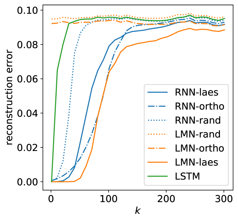
Figure 2(b) shows the reconstruction error for different architectures and initializations. A linear model is trained to reconstruct the hidden activations given , with a separate model trained for each . We plot the average reconstruction error for each configuration. The LMN with LAES initialization obtains the best performance for both short-term and long-term reconstruction. Classic models such as the LSTM and orthogonal models obtain worse reconstructions.
6 Conclusion
In this work, we propose the maximization of the STM capacity as an alternative objective to encourage learning long-term dependencies with recurrent neural networks. Maximizing the STM is a difficult problem due to the presence of long-term dependencies. We show that RNN models trained with BP fail to encode simple but long sequences. To address this issue, we propose to initialize recurrent models with a linear autoencoder for sequences. The LAES can be trained without BP and efficiently encodes long sequences, unlike RNNs trained with BP. As a future work, we plan to improve the proposed method to completely remove the BP step through the recurrent units.
References
- Arjovsky et al. (2015) M. Arjovsky, A. Shah, and Y. Bengio. Unitary evolution recurrent neural networks. In ICML, 2015.
- Arpit et al. (2018) D. Arpit, B. Kanuparthi, G. Kerg, Nan R. Ke, I. Mitliagkas, and Y. Bengio. h-detach: Modifying the lstm gradient towards better optimization. ArXiv, abs/1810.03023, 2018.
- Bacciu et al. (2019) D. Bacciu, A. Carta, and A. Sperduti. Linear Memory Networks. In ICANN, 2019.
- Bengio et al. (1994) Yoshua Bengio, Patrice Simard, and Paolo Frasconi. Learning long-term dependencies with gradient descent is difficult. IEEE transactions on neural networks, 5(2):157–166, 1994.
- Carta et al. (2020a) Antonio Carta, Alessandro Sperduti, and Davide Bacciu. Encoding-based Memory Modules for Recurrent Neural Networks. arXiv:2001.11771 [cs, stat], January 2020.
- Carta et al. (2020b) Antonio Carta, Alessandro Sperduti, and Davide Bacciu. Incremental Training of a Recurrent Neural Network Exploiting a Multi-Scale Dynamic Memory. arXiv:2006.16800 [cs, stat], June 2020.
- Casado and Martínez-Rubio (2019) M. Lezcano Casado and D. Martínez-Rubio. Cheap orthogonal constraints in neural networks: A simple parametrization of the orthogonal and unitary group. In ICML, 2019.
- Chang et al. (2019) B. Chang, M. Chen, E. Haber, and Ed H. Chi. Antisymmetricrnn: A dynamical system view on recurrent neural networks. ArXiv, abs/1902.09689, 2019.
- Ganguli et al. (2008) S. Ganguli, D. Huh, and H. Sompolinsky. Memory Traces in Dynamical Systems - Supplementary Material Contents. Proceedings of the National Academy of Sciences, 2008.
- Hochreiter and Schmidhuber (1997) S.; Hochreiter and J.; Schmidhuber. Long Short-Term Memory. Neural Computation, 9(8):1–32, 1997.
- Hochreiter (1998) Sepp Hochreiter. The vanishing gradient problem during learning recurrent neural nets and problem solutions. International Journal of Uncertainty, Fuzziness and Knowledge-Based Systems, 6(02):107–116, 1998.
- Jaeger and Haas (2004) H. Jaeger and H. Haas. Harnessing nonlinearity: Predicting chaotic systems and saving energy in wireless communication. science, 304(5667), 2004.
- Jing et al. (2016) L. Jing, Y. Shen, T. Dubček, J. Peurifoy, S. Skirlo, Y. LeCun, M. Tegmark, and M. Soljačić. Tunable Efficient Unitary Neural Networks (EUNN) and their application to RNNs. In ICML, 2016.
- Jose et al. (2018) C. Jose, M. Cissé, and F. Fleuret. Kronecker Recurrent Units. In ICML, may 2018.
- Kingma and Ba (2014) D. P. Kingma and J. Ba. Adam: A Method for Stochastic Optimization. arXiv preprint arXiv:1412.6980, 2014.
- Krueger and Memisevic (2015) D. Krueger and R. Memisevic. Regularizing rnns by stabilizing activations. CoRR, abs/1511.08400, 2015.
- Le et al. (2015) Quoc V Le, N. Jaitly, and G. E Hinton. A simple way to initialize recurrent networks of rectified linear units. arXiv preprint arXiv:1504.00941, 2015.
- LeCun (1998) Yann LeCun. The MNIST database of handwritten digits. http://yann. lecun. com/exdb/mnist/, 1998.
- Mhammedi et al. (2017) Z. Mhammedi, A. Hellicar, A. Rahman, and J. Bailey. Efficient Orthogonal Parametrisation of Recurrent Neural Networks Using Householder Reflections. In ICML, 2017.
- Pasa and Sperduti (2014) L. Pasa and A. Sperduti. Pre-training of Recurrent Neural Networks via Linear Autoencoders. NIPS, 2014.
- Sperduti (2006) A. Sperduti. Exact Solutions for Recursive Principal Components Analysis of Sequences and Trees. In ICANN, 2006.
- Sperduti (2007) A. Sperduti. Efficient computation of recursive principal component analysis for structured input. In ECML, 2007.
- Sperduti (2013) Alessandro Sperduti. Linear autoencoder networks for structured data. In International Workshop on Neural-Symbolic Learning and Reasoning, 2013.
- Tino et al. (2004) P. Tino, M. Cernansky, and L. Benuskova. Markovian Architectural Bias of Recurrent Neural Networks. IEEE Transactions on Neural Networks, 2004.
- Tiňo and Rodan (2013) P Tiňo and A Rodan. Short term memory in input-driven linear dynamical systems. Neurocomputing, 112:58–63, 2013.
- Vorontsov et al. (2017) E. Vorontsov, C. Trabelsi, S. Kadoury, and C. Pal. On orthogonality and learning recurrent networks with long term dependencies. In ICML, 2017.
- White et al. (2004) O. L. White, D. Lee, and H. Sompolinsky. Short-term memory in orthogonal neural networks. Physical Review Letters, 92(14):0–3, 2004.
- Wisdom et al. (2016) S. Wisdom, T. Powers, J. R. Hershey, J. Le Roux, and L. Atlas. Full-Capacity Unitary Recurrent Neural Networks. In NIPS, 2016.
- Zhang et al. (2018) J. Zhang, Q. Lei, and I. Dhillon. Stabilizing Gradients for Deep Neural Networks via Efficient SVD Parameterization. In ICML, 2018.
Appendix A Related Work
Orthogonal RNNs solve the vanishing gradient problem by parameterizing the recurrent connections with an orthogonal or unitary matrix Arjovsky et al. [2015]. Some orthogonal models exploit specific parameterizations or factorizations Mhammedi et al. [2017]; Jose et al. [2018]; Jing et al. [2016] to guarantee the orthogonality. Other approaches constrain the parameters with soft or hard orthogonality constraints Vorontsov et al. [2017]; Zhang et al. [2018]; Wisdom et al. [2016]; Casado and Martínez-Rubio [2019]. Vorontsov et al. [2017] have shown that hard orthogonality constraints can hinder training speed and final performance.
Linear autoencoders for sequences can be trained optimally with a closed-form solution Sperduti [2013]. They have been used to pretrain RNNs Pasa and Sperduti [2014]. The LMN Bacciu et al. [2019] is a recurrent neural network with a separate linear recurrence, which can be exploited to memorize long sequences by pretraining it with the LAES Carta et al. [2020a, b].
The memorization properties of untrained models are studied in the field of echo state echo networks Jaeger and Haas [2004], a recurrent model with untrained recurrent parameters. Tino et al. [2004] showed that untrained RNNs with a random weight initialization have a Markovian bias, which results in the clustering of input with similar suffixes in the hidden state space. Tiňo and Rodan [2013]; White et al. [2004]; Ganguli et al. [2008] study the short-term memory properties of linear and orthogonal memories.
Appendix B Sequential and Permuted MNIST experiments
Sequential and permuted MNIST Le et al. [2015] are two standard benchmarks designed to test the ability of recurrent neural networks to learn long-term dependencies. They consist of sequences extracted from the MNIST dataset LeCun [1998] by scanning each image one pixel at a time, in order (sequential MNIST) or with a random fixed permutation (permuted MNIST). We use these datasets to compare the LAES initialization to a random orthogonal initialization, since they provide an ideal setting to test a pure memorization approach like the LAES initialization. All the models have hidden units and a single hidden layer. Each model has been trained for epochs with a batch size of .
Each model is trained with Adam Kingma and Ba [2014], with a learning rate in chosen by selecting the best model on a separate validation set. A soft orthogonality constraint is added to the cost function as in Vorontsov et al. [2017], with chosen . We apply the activation regularization proposed in Krueger and Memisevic [2015], with . To apply the stochastic gradient truncation Arpit et al. [2018] we select the probability of truncation , which includes the full backpropagation() and the exact truncation ().
B.1 Baseline Models
We compare against orthogonal and unitary RNNs, which are recurrent models with unitary recurrent matrices that guarantee constant gradient propagationArjovsky et al. [2015], such as the FC uRNNWisdom et al. [2016], EURNNJing et al. [2016], KRUJose et al. [2018]. We also compare against the LSTMHochreiter and Schmidhuber [1997], and ASRNNChang et al. [2019].
We study different baseline that exploit the LAES to verify if the backpropagation through the hidden units is necessary:
- LAES-Linear
-
A LAES with a linear classifier trained by pseudoinverse. The model does not use backpropagation.
- LAES-SVM
-
A LAES with an SVM classifier. The model does not use backpropagation.
- LAES-FF
-
A LAES with a feedforward classifier. The model uses truncated backpropagation, propagating the gradient only through the feedforward units, leaving the recurrent connections fixed.
Appendix C MNIST Sequence Reconstruction
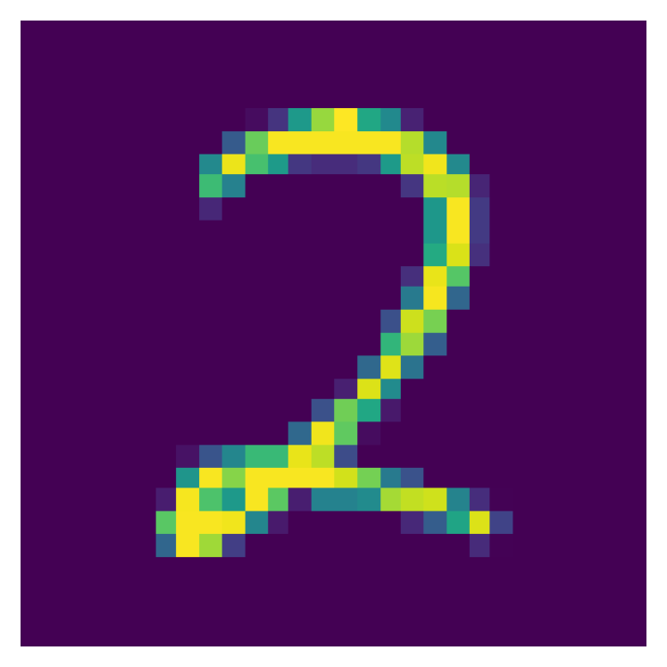
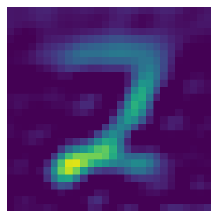
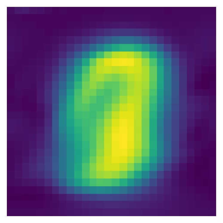
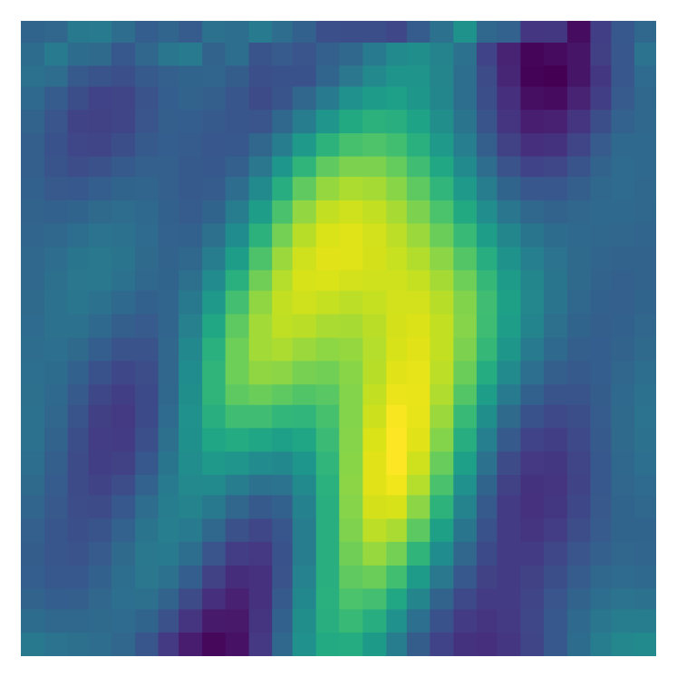
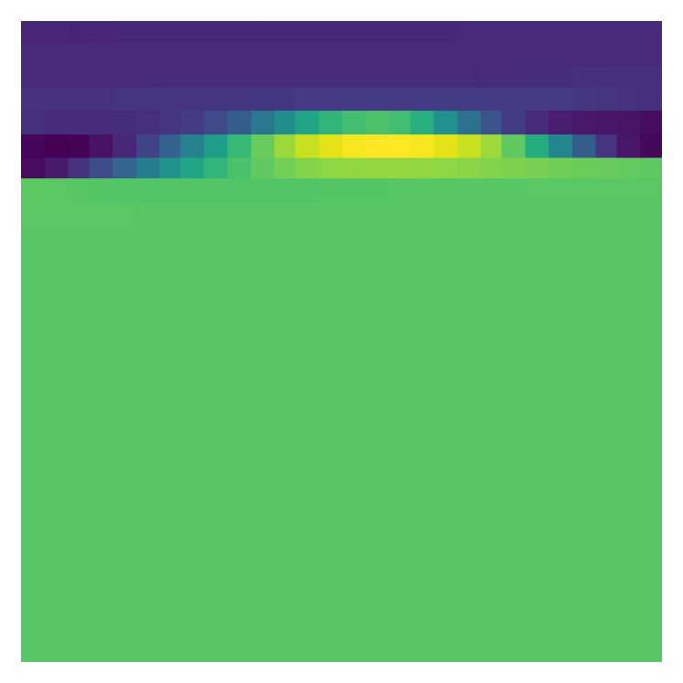
We trained different recurrent models to reconstruct Sequential MNIST samples. Each model consists of a single layer RNN with hidden units. We compare the Elman RNN, LSTM, RNN with orthogonal initialization, and the LAES. Except for the LAES, each model has been trained for epochs with backpropagation, using Adam Kingma and Ba [2014], with a learning rate chosen with a separate validation set in . For the orthogonal RNN we add a soft orthogonality constraint by penalizing the recurrent weight matrix as in Vorontsov et al. [2017], chosen from the values in . Figure 3 shows a sample reconstruction for each model. The only model which is able to approximately reconstruct the original image is the LAES, which is also the only one not trained with backpropagation.