Imperial-TP-AT-2020-06

On the structure of non-planar strong coupling corrections to correlators of BPS Wilson loops and chiral primary operators

M. Beccaria${}^{\,a}$ and A.A. Tseytlin${}^{\,b,}$

^a Università del Salento, Dipartimento di Matematica e Fisica Ennio De Giorgi,

and I.N.F.N. - sezione di Lecce, Via Arnesano, I-73100 Lecce, Italy ^b Blackett Laboratory, Imperial College London SW7 2AZ, U.K.

E-mail: matteo.beccaria@le.infn.it,   tseytlin@imperial.ac.uk

Starting with some known localization (matrix model) representations for correlators involving 1/2 BPS circular Wilson loop $\cal W$ in ${\cal N}=4$ SYM theory we work out their $1/N$ expansions in the limit of large ’t Hooft coupling $\lambda$. Motivated by a possibility of eventual matching to higher genus corrections in dual string theory we follow arXiv:2007.08512 and express the result in terms of the string coupling $g_{\rm s}\sim g^{2}_{\rm YM}\sim\lambda/N$ and string tension $T\sim\sqrt{\lambda}$. Keeping only the leading in $1/T$ term at each order in $g_{\rm s}$ we observe that while the expansion of $\langle{\cal W}\rangle$ is a series in $g^{2}_{\rm s}/T$, the correlator of the Wilson loop with chiral primary operators ${\cal O}_{J}$ has expansion in powers of $g^{2}_{\rm s}/T^{2}$. Like in the case of $\langle{\cal W}\rangle$ where these leading terms are known to resum into an exponential of a “one-handle” contribution $\sim g^{2}_{\rm s}/T$, the leading strong coupling terms in $\langle{\cal W}\,{\cal O}_{J}\rangle$ sum up to a simple square root function of $g^{2}_{\rm s}/T^{2}$. Analogous expansions in powers of $g^{2}_{\rm s}/T$ are found for correlators of several coincident Wilson loops and they again have a simple resummed form. We also find similar expansions for correlators of coincident 1/2 BPS Wilson loops in the ABJM theory.

1 Introduction and summary

An important direction is to extend checks of AdS/CFT correspondence to subleading orders in $1/N$ expansion on the gauge theory side or higher genus corrections on the dual string theory side. One of the simplest observables to consider is the expectation value $\langle\mathcal{W}\rangle$ of $1\over 2$-BPS circular Wilson loop for which the exact in $N$ expressions are available in both $SU(N)$ $\mathcal{N}=4$ SYM [1, 2, 3, 4] and $U(N)_{k}\times U(N)_{-k}$ ABJM [5, 6, 7] theories. It was recently observed in [8] that the expressions for $\langle\mathcal{W}\rangle$ expanded first in $1/N$ and then in large ’t Hooft coupling $\lambda$ have a universal form when written in terms of the corresponding string coupling $g_{\rm s}$ and string tension $T={{\rm R}^{2}\over 2\pi\alpha^{\prime}}$ defined as [9, 10]

$${\rm SYM}:\qquad g_{{\rm s}}=\frac{g^{2}_{\rm YM}}{4\pi}=\frac{\lambda}{4\pi N}\ ,\qquad\lambda=g^{2}_{\rm YM}N\ ,\qquad T={\sqrt{\lambda}\over 2\pi}\ ,$$ (1.1)

$${\rm ABJM}:\qquad g_{{\rm s}}={\sqrt{\pi}\,(2\lambda)^{5/4}\over N}\ ,\qquad\lambda={N\over k}\ ,\qquad\ \ \ \ \ T={\sqrt{2\lambda}\over 2}\ .$$ (1.2)

Explicitly,

$$\langle\mathcal{W}\rangle= \ e^{2\pi\,T}\sum^{\infty}_{p=0}\text{c}_{p}\Big{(}\frac{g_{\rm s}}{\sqrt{T}}\Big{)}^{2p-1}\,\Big{[}1+\mathcal{O}(T^{-1})\Big{]}$$

$$= \ e^{2\pi\,T}\,{\sqrt{T}\over g_{\rm s}}\Big{\{}\text{c}_{0}\big{[}1+{\cal O}(T^{-1})\big{]}+\text{c}_{1}{g^{2}_{\rm s}\over T}\big{[}1+{\cal O}(T^{-1})\big{]}+\text{c}_{2}\Big{(}{g^{2}_{\rm s}\over T}\Big{)}^{2}\big{[}1+{\cal O}(T^{-1})\big{]}+...\Big{\}}\ .$$ (1.3)

Indeed, this is what one finds by expanding (in large $N$ and then in large $\lambda$) the exact result in, e.g., SYM theory [2]

$$\langle\mathcal{W}\rangle =e^{\frac{\lambda}{8N}}\,L_{N-1}^{(1)}\big{(}-\frac{\lambda}{4N}\big{)}=N\,e^{\sqrt{\lambda}}\sum_{p=0}^{\infty}\frac{\sqrt{2}}{96^{p}\sqrt{\pi}p!}\frac{\lambda^{\frac{6p-3}{4}}}{N^{2p}}\Big{[}1+\mathcal{O}\big{(}\frac{1}{\sqrt{\lambda}}\big{)}\Big{]}\ ,$$ (1.4)

i.e. we get (1.3) with $c_{0}=\frac{1}{2\pi}$, $c_{1}=\frac{1}{24}$, etc. The universal structure of (1.3) is a manifestation of the fact that the two gauge theories are expected to be dual to similar superstring theories in ${\rm AdS}_{5}\times S^{5}\$and ${\rm AdS}_{4}\times CP^{3}$ where $\langle\mathcal{W}\rangle$ should be given by a string path integral over surfaces ending on a circle at the boundary of AdS. $e^{2\pi\,T}$ in (1.3) is the semiclassical factor corresponding to an AdS₂ minimal surface [11, 12, 13]. The expansion is done first in small string coupling $g_{\rm s}$ (i.e. large $N$ for fixed $T\sim\sqrt{\lambda}$) and then in $1/T$ at each order in $g_{\rm s}$. The power of string coupling is the Euler number $\chi=1-2p$ of a disc with $p=0,1,2,...$ handles.

A non-trivial feature of (1.3) is that the leading power of the inverse string tension $1/T$ at each order in $g_{\rm s}$ is precisely $-{1\over 2}\chi=p-{1\over 2}$, i.e. it is correlated with the power of $g_{\rm s}$. A string theory explanation of this fact was suggested in [8] by showing that dependence of the string partition function on the AdS_n radius ${\rm R}$ (and thus on the string tension) is controlled by the Euler number of the surface.

Another remarkable fact about the SYM result (1.4) is that the leading large $T$ terms in (1.3) exponentiate [2] (according to (1.4), the coefficients $\text{c}_{p}$ in (1.3) are given by $\text{c}_{p}=\frac{1}{2\pi p!}\big{(}\frac{\pi}{12}\big{)}^{p}$)

$$\langle\mathcal{W}\rangle={1\over 2\pi}\frac{\sqrt{T}}{g_{\text{s}}}\,e^{2\pi\,T\ +\ \frac{\pi}{12}\frac{g_{\text{s}}^{2}}{T}}\,\Big{[}1+\mathcal{O}(T^{-1})\Big{]}\ .$$ (1.5)

Surprisingly, in the ABJM theory the coefficient of the first subleading correction is the same $\pi\over 12$ as in the SYM case [7]

$$\langle\mathcal{W}\rangle=\Big{(}\frac{N}{4\pi\,\lambda}+\frac{\pi\,\lambda}{6N}+\cdots\Big{)}\,e^{\pi\,\sqrt{2\lambda}}={1\over\sqrt{2\pi}}\frac{\sqrt{T}}{g_{\text{s}}}\,e^{2\pi\,T}\Big{[}1+\frac{\pi}{12}\,\frac{g_{\text{s}}^{2}}{T}+{\cal O}(g^{4}_{s})\Big{]}\ .$$ (1.6)

However, the coefficients of higher order terms (that can be found from [14]) turn out to be different than in the SYM case (1.4), i.e. here the exponentiation does not happen. Instead, we will find (see Appendix  E) that in the ABJM case the leading strong-coupling terms in (1.3) can be resummed as

$$\langle\mathcal{W}\rangle={1\over 2\sin[\sqrt{\frac{\pi}{2}}\,\frac{g_{\text{s}}}{\sqrt{T}}]}\,e^{2\pi\,T}\Big{[}1+\mathcal{O}(T^{-1})\Big{]}\ ,$$ (1.7)

where $\sqrt{\frac{\pi}{2}}\,\frac{g_{\text{s}}}{\sqrt{T}}=2\pi\,\frac{\lambda}{N}={2\pi\over k}$ (see (1.2)).

Our aim below will be to extract similar predictions about the structure of small $g_{\rm s}$, large $T$ string theory corrections and their possible resummation for other closely related observables for which the exact gauge theory results can be found from matrix model representations following from localization (in some cases generalizing partial results in the literature).

Namely, we shall consider correlators of ${1\over 2}$-BPS Wilson loop with chiral primary operators (CPO) and also correlators of several coincident Wilson loops (mostly in the SYM theory). Like in the case of $\langle\mathcal{W}\rangle$ in (1.3) we will observe certain universal patterns in their expansion in small $g_{\rm s}$ and large $T$ that should be related to supersymmetry of these observables. This may hopefully aid future investigations on the dual string theory side.

Let us summarize our main results.

1.1 Correlators of $\frac{1}{2}$-BPS Wilson loop with chiral primary operators

In section 2 we shall consider the SYM correlator of a circular Wilson loop with a chiral primary operator $\mathcal{O}_{J}=\operatorname{\text{tr}}\varphi^{J}$. The correlator $\langle\mathcal{W}\,\mathcal{O}_{J}\rangle$ was originally discussed in [11] at the leading order in strong coupling in connection with the Wilson loop OPE expansion. In the planar limit this correlator was computed exactly in $\lambda$ in [20]: $\langle\mathcal{W}\,\mathcal{O}_{J}\rangle\sim I_{J}(\sqrt{\lambda})$ ($I_{J}$ is the Bessel function).

We have extended the computation to non-planar corrections; expanded in small $g_{\rm s}$ and then in large $T$ as in (1.3) the result reads

$$\frac{\langle\mathcal{W}\,\mathcal{O}_{J}\rangle}{\langle\mathcal{W}\rangle}=c_{J}\,T\,\Big{\{}1 +\frac{a_{0}^{(1)}(J)}{T}+\frac{a_{0}^{(2)}(J)}{T^{2}}+\cdots+\frac{g_{\text{s}}^{2}}{T^{2}}\,\Big{[}a_{1}^{(0)}(J)+\frac{a_{1}^{(1)}(J)}{T}+\cdots\Big{]}$$

$$+\frac{g_{\text{s}}^{4}}{T^{4}}\,\Big{[}a_{2}^{(0)}(J)+\frac{a_{2}^{(1)}(J)}{T}+\cdots\Big{]}+{\cal O}\Big{(}\frac{g_{\text{s}}^{6}}{T^{6}}\Big{)}\Big{\}}\ ,$$ (1.8)

where dots stand for terms subleading in $1/T$. On the string theory side, the overall factor of $T$ should come from the semiclassical value of the vertex operator dual to ${\cal O}_{J}$ evaluated on the AdS₂ minimal surface. The coefficient $c_{J}$ is fixed by normalization of $\mathcal{O}_{J}$ and $a_{i}^{(j)}(J)$ are polynomials in $J$, cf. (2.4) (for example, $a_{0}^{(1)}=-{1\over 4\pi}(J^{2}-1)$ as in [20]). Compared to the series in $\frac{g_{\text{s}}^{2}}{T}\sim\frac{\lambda^{3/2}}{N^{2}}$ in (1.3) here the natural expansion parameter turns out to be $x\equiv\frac{g_{\text{s}}^{2}}{T^{2}}\sim\frac{\lambda}{N^{2}}$.

Remarkably, it is possible to explicitly sum up all leading large $T$ terms in (1.1) as

$$\frac{\langle\mathcal{W}\,\mathcal{O}_{J}\rangle}{\langle\mathcal{W}\rangle}=c_{J}\,T\,F_{J}\Big{(}\frac{g_{\text{s}}^{2}}{T^{2}}\Big{)}\,\Big{[}1+{\cal O}(T^{-1})\Big{]}\ ,\qquad\qquad F_{J}(x)=\frac{2}{J\sqrt{x}}\sinh\Big{(}J\,\text{arcsinh}\frac{\sqrt{x}}{2}\Big{)}.$$ (1.9)

Here $F_{J}$ is a finite polynomial for odd $J$ and $\sqrt{1+\tfrac{1}{4}{g_{\text{s}}^{2}\over T^{2}}}$ times a polynomial for even $J$. For example, in the $J=2$ case one finds simply

$$\frac{\langle\mathcal{W}\,\mathcal{O}_{2}\rangle}{\langle\mathcal{W}\rangle}=\pi\,\sqrt{T^{2}+\tfrac{1}{4}g_{\text{s}}^{2}}\,\Big{[}1+\mathcal{O}\Big{(}T^{-1}\Big{)}\Big{]}.$$ (1.10)

The same expression applies also to the correlator of $\mathcal{W}$ with the dimension 4 dilaton operator $\mathcal{O}_{\rm dil}$ which is a supersymmetry descendant of ${\cal O}_{2}$. For any $g_{\rm s}$ and $T$ the expectation value $\frac{\langle\mathcal{W}\,\mathcal{O}_{\rm dil}\rangle}{\langle\mathcal{W}\rangle}$ can be found directly from $\langle\mathcal{W}\rangle$ in (1.3),(1.4) by differentiating over $\lambda$ so that using (1.1) we have (see [8] and refs. there)

$$\frac{\langle\mathcal{W}\,\mathcal{O}_{2}\rangle}{\langle\mathcal{W}\rangle}=\frac{\langle\mathcal{W}\,\mathcal{O}_{\rm dil}\rangle}{\langle\mathcal{W}\rangle}=\lambda{\partial\over\partial\lambda}\log\langle\mathcal{W}\rangle=\Big{(}{1\over 2}T{\partial\over\partial T}+g_{\rm s}{\partial\over\partial g_{\rm s}}\Big{)}\log\langle\mathcal{W}\rangle\ .$$ (1.11)

The small $g_{\text{s}}$, large $T$ expansion of $\log\langle\mathcal{W}\rangle$ following from (1.4) is found to be

$$\log\langle\mathcal{W}\rangle=2\pi T -{1\over 2}\log\Big{(}4\pi^{2}{g^{2}_{\rm s}\over T}\Big{)}-\frac{3}{16\pi T}+\cdots+\frac{\pi}{12}\frac{g_{\text{s}}^{2}}{T}\,\Big{(}1-\frac{3}{4\pi T}+\cdots\Big{)}$$

$$-\frac{\pi}{320}\frac{g_{\text{s}}^{4}}{T^{3}}\,\Big{(}1-\frac{1945}{768\pi T}+\cdots\Big{)}+\mathcal{O}\Big{(}{g_{\text{s}}^{6}\over T^{5}}\Big{)}\ ,$$ (1.12)

and therefore

$$\Big{(}{1\over 2}T{\partial\over\partial T}+g_{\rm s}{\partial\over\partial g_{\rm s}}\Big{)}\log\langle\mathcal{W}\rangle=\pi\,T\,\Big{[}1 -\frac{3}{4\pi T}+\cdots+\frac{g_{\text{s}}^{2}}{8\,T^{2}}\Big{(}1-\frac{1}{2\pi T}+\cdots\Big{)}$$

$$-\frac{g_{\text{s}}^{4}}{128\,T^{4}}\Big{(}1-\frac{389}{192\pi T}+\cdots\Big{)}+\mathcal{O}\Big{(}{g_{\text{s}}^{6}\over T^{6}}\Big{)}\Big{]}\ ,$$ (1.13)

in agreement with (1.1). The reason why the large $T$ expansion (1.1) has a different structure than (1.3) and thus also why the resummed expressions in (1.5) and in (1.10) are not directly related by (1.11) is that subleading in $1/T$ terms at each order in $g_{\rm s}$ in $\langle\mathcal{W}\rangle$ in (1.3) contribute to $\log\langle\mathcal{W}\rangle$ and, as a result, reorganize its large $T$ expansion (see (2.45)–(2.4.2) for details).

There is still an interesting connection between the resummed expressions for $\langle\mathcal{W}\rangle$ in (1.5) and the correlator ${\langle\mathcal{W}\,\mathcal{O}_{2}\rangle}$ in (1.9),(1.10): both can be given a “D3-brane” interpretation [31, 28]. To recall, for a circular Wilson loop in $k$-symmetric $SU(N)$ representation in the limit of large $k,\,N$ and $\lambda$ with $\varkappa={k\sqrt{\lambda}\over 4N}={k\,g_{\rm s}\over 2\,T}=$fixed one expects that $\langle\mathcal{W}\rangle$ should be given by $\exp(-S_{\rm D3})$ where $S_{\rm D3}$ is the D3-brane action on the corresponding classical solution [31]. For $1\ll k\ll N$ this should apply also to the Wilson loop in the $k$-fundamental representation described by a minimal surface ending on a multiply wrapped circle; here one finds [31]:   $S_{\rm D3}=Nf(\varkappa)=-k\sqrt{\lambda}-{k^{3}\lambda^{3/2}\over 96N^{2}}+{\cal O}({k^{5}\lambda^{5/2}\over N^{4}})$. Extrapolating this to the $k=1$ case corresponds to the resummation of the expansion in (1.3),(1.4) for fixed ${\sqrt{\lambda}\over N}\sim{g_{\rm s}\over T}$ (i.e. when $g_{\rm s}\sim T$ formally are both large, cf. [31, 32]). Then $S_{\rm D3}=-2\pi T-{\pi\over 12}\,{g^{2}_{\rm s}\over T}+{\cal O}({g^{4}_{\rm s}\over T^{3}})$, reproducing the exponential factor in (1.5). Similar D3-brane interpretation is possible also in the case of the correlator ${\langle\mathcal{W}\,\mathcal{O}_{J}\rangle}$ [28]. Indeed, the resummed expression (1.9) is in perfect agreement with the result found in [28] in the fixed $\varkappa={k\,g_{\rm s}\over 2\,T}$ limit (both from the derivative of the D3-brane action over the corresponding graviton source and from the matrix model in the case of $k$-fundamental representation) after formally interpolating to the $k=1$ case.

In section 3 we shall also consider the correlator $\langle\mathcal{W}\,\mathcal{O}_{J_{1}}\,\mathcal{O}_{J_{2}}\rangle$ with two chiral primary operators. In the two special cases (a) $J_{1}=J_{2}$ and (b) $J_{1}=2,J_{2}=2J$ it is possible to reduce their computation to correlators in the Gaussian 1-matrix model. The structure of the resulting $1/N$ strong coupling expansion is found to be similar to (1.1)

$$\frac{\langle\mathcal{W}\,\mathcal{O}_{J_{1}}\,\mathcal{O}_{J_{2}}\rangle}{\langle\mathcal{W}\rangle}=d_{J_{1}J_{2}}\,T^{2}\,\Big{\{}1+\frac{b_{0}^{(1)}(J_{1},J_{2})}{T}+\frac{b_{0}^{(2)}(J_{1},J_{2})}{T^{2}}+\cdots$$ (1.14)

$$\quad+\frac{g_{\text{s}}^{2}}{T^{2}}\,\Big{[}b_{1}^{(0)}(J_{1},J_{2})+\frac{b_{1}^{(1)}(J_{1},J_{2})}{T}+\cdots\Big{]}+\frac{g_{\text{s}}^{4}}{T^{4}}\,\Big{[}b_{2}^{(0)}(J_{1},J_{2})+\frac{b_{2}^{(1)}(J_{1},J_{2})}{T}+\cdots\Big{]}+{\cal O}\Big{(}{g^{6}_{\rm s}\over T^{6}}\Big{)}\Big{\}},$$

where $b_{i}^{(j)}$ are polynomials in $J_{1},J_{2}$ (see (3.1),(3.22),(3.23)).

1.2 Correlators of coincident Wilson loops

Another class of tractable examples that we shall consider in section 4 are the expectation values of coincident circular Wilson loops $\langle\mathcal{W}^{n}\rangle$ in SYM theory. The $n=2$ case in the planar limit was discussed, in particular, in [2, 44]. Extending calculation to subleading orders in $1/N$ in large $\lambda$ limit and rewriting the resulting expansion in terms of $g_{\rm s}$ and $T$ as in (1.3) we have found that

$$\frac{\langle\mathcal{W}^{2}\rangle}{\langle\mathcal{W}\rangle^{2}}= \sum_{p=0}^{\infty}\frac{\pi^{p}}{(2p-1)!!}\Big{(}{g_{\rm s}\over T}\Big{)}^{p}\Big{[}1+\mathcal{O}(T^{-1})\Big{]}$$

$$= 1+e^{\frac{\xi}{2}}\sqrt{\frac{\pi\,\xi}{2}}\,\text{erf}\Big{(}\sqrt{\frac{\xi}{2}}\Big{)}+\mathcal{O}(T^{-1}),\ \ \ \ \ \qquad\xi\equiv\pi\frac{g^{2}_{\rm s}}{T}\ .$$ (1.15)

The analogous expression for $n=3$ is

$$\frac{\langle\mathcal{W}^{3}\rangle}{\langle\mathcal{W}\rangle^{3}}=1+3e^{\frac{\xi}{2}}\sqrt{\frac{\pi\,\xi}{2}}\,\text{erf}\Big{(}\sqrt{\frac{\xi}{2}}\Big{)}+\frac{4\pi}{3\sqrt{3}}\,\xi\,e^{2\xi}\,\Big{[}1-12\,{\rm T}\Big{(}\sqrt{3\xi},\frac{1}{\sqrt{3}}\Big{)}\Big{]}+\mathcal{O}(T^{-1}),$$ (1.16)

where ${\rm T}(h,a)$ is the Owen T-function (see (4.40)). For general $n$ we found similar expansion (see (4.42) and Appendix D)

$$\frac{\langle\mathcal{W}^{n}\rangle}{\langle\mathcal{W}\rangle^{n}}=1 +\frac{n\,(n-1)}{2}\,\xi+\frac{\,n(n-1)(3n-5)\,(n+2)}{24}\,\xi^{2}$$

$$+\frac{\,n(n-1)(15n^{4}+30n^{3}-75n^{2}-610n+1064)}{720}\,\xi^{3}+...\ .$$ (1.17)

Thus like for $\langle{\cal W}\rangle$ in (1.3) here we get again series in $\xi=\pi\frac{g^{2}_{\rm s}}{T}$ while for the correlators with chiral primary operators (1.1),(1.14) the expansion was in powers of $x={g^{2}_{s}\over T^{2}}$.

In section 4.3 we shall derive a similar expansion for the correlator $\mathcal{W}^{(1,-1)}$ of coincident Wilson loops in fundamental and anti-fundamental representations. It turns out that in contrast to (1.2),(1.2) $\mathcal{W}^{(1,-1)}$ has trivial connected part, i.e. to all orders in $\xi$ (and to leading order in $1/T$)

$$\langle{\mathcal{W}^{(1,-1)}}\rangle=\langle\mathcal{W}\rangle^{2}\,\Big{[}1+\mathcal{O}(T^{-1})\Big{]}\simeq\langle\mathcal{W}\rangle^{2}\ .$$ (1.18)

It would be interesting to explain this fact from the string theory point of view.

1.3 Comments on correlators in ABJM

Obtaining the above results in the ${\cal N}=4$ SYM theory case is facilitated by a relative simplicity of the associated Gaussian matrix model. In the ABJM theory the computations of similar correlators involving $\frac{1}{2}$-BPS circular Wilson loop [45] are substantially more involved.

The structure of the strong-coupling expansion of the correlators with chiral primary operators is expected to be similar to (1.1). This is suggested by the observation [8] that the expansion (1.3) of $\langle\mathcal{W}\rangle$ looks the same in the SYM and ABJM theories and that, in particular, for the dilaton operator the correlators $\langle\mathcal{W}\,\mathcal{O}_{\rm dil}\rangle$ and $\langle\mathcal{W}\rangle$ should be again related as in the last equality in (1.11). Indeed, the dilaton vertex operator has the same structure in both ${\rm AdS}_{5}\times S^{5}\$and AdS${}_{4}\times CP^{3}$ string theories and thus the derivative over the zero-momentum dilaton should be related to the string partition function in the same way as in ${\rm AdS}_{5}\times S^{5}\$case in [8], i.e. as in (1.11).

Below in Appendix F we shall discuss the computation of correlators of coincident Wilson loops $\langle{\mathcal{W}}^{n}\rangle$ in ABJM theory. In particular, for the $n=2,3$ we will find

$$\langle\mathcal{W}^{2}\rangle=\langle\mathcal{W}\rangle^{2}\,\Big{[}1+0\times\frac{g_{\text{s}}^{2}}{T}+0\times\Big{(}\frac{g_{\text{s}}^{2}}{T}\Big{)}^{2}+\cdots\Big{]},\qquad\langle\mathcal{W}^{3}\rangle=\langle\mathcal{W}\rangle^{3}\,\Big{[}1+0\times\frac{g_{\text{s}}^{2}}{T}+0\times\Big{(}\frac{g_{\text{s}}^{2}}{T}\Big{)}^{2}+\cdots\Big{]},$$ (1.19)

suggesting the conjecture that, up to subleading $1/T$ terms at each order in the genus expansion, here the connected part of the correlator $\langle\mathcal{W}^{n}\rangle$ vanishes, i.e. $\langle\mathcal{W}^{n}\rangle\simeq\langle\mathcal{W}\rangle^{n}$. This is in contrast to the non-trivial relation (1.2) found for $\langle\mathcal{W}^{n}\rangle$ in the SYM case (but is similar to the behaviour of $\langle{\mathcal{W}^{(1,-1)}}\rangle$ in (1.18)).

1.4 Structure of the paper

In section 2 we compute the $1/N$ expansion (1.1) of the SYM correlator $\langle\mathcal{W}\,\mathcal{O}_{J}\rangle$ of the $\frac{1}{2}$-BPS Wilson loop with a chiral primary operator starting with its matrix model representation implied by localization. In section 3 we repeat the same analysis for the correlator $\langle\mathcal{W}\,\mathcal{O}_{J_{1}}(x_{1})\mathcal{O}_{J_{2}}(x_{2})\rangle$ assuming a special (supersymmetric) choice of insertion points $x_{1}$ and $x_{2}$ that allows a matrix model calculation confirming that its strong coupling expansion has the form (1.14).

In section 4 we consider correlators of coincident BPS Wilson loops. We establish the structure of the expansions in (1.2),(1.16) and prove their exact form by exploiting the Toda integrability structure of the underlying Gaussian matrix model. In section 4.3 we consider the correlator of Wilson loops in the fundamental and in the anti-fundamental representation where special features are expected due to supersymmetry. Indeed, in this case one finds (1.1), i.e. there are no leading order corrections to $\mathcal{W}^{(1,-1)}$ beyond those in $\langle\mathcal{W}^{2}\rangle$.

In Appendix A we discuss an attempt [2] to explain the negative power of $T$ in the ${g_{\text{s}}^{2}}/{T}$ term in (1.3) by assuming that for large $T$ one can use supergravity approximation as in [11]. As we explain, this argument may work only if there are non-trivial cancellations of the dominant large $T$ terms that should be implied by supersymmetry. Appendix B contains some technical details of the $1/N$ expansion of $\langle\mathcal{W}\rangle$. In Appendix C we consider the $1/N$ expansion of the correlator $\langle{\cal W}\,\mathcal{O}_{J}\rangle$ in the string semiclassical limit $J\sim\sqrt{\lambda}\gg 1$. In Appendix D we work out the $1/N$ expansion of $\langle\mathcal{W}^{n}\rangle$ deriving the expansion (1.2).

The Appendices E and F are devoted to the correlators $\langle\mathcal{W}^{n}\rangle$ of $\frac{1}{2}$-BPS circular Wilson loop in the ABJM theory. In Appendix E we comment on the single Wilson loop case case by reviewing the known matrix model results pointing out that here the expansion has again the same structure as in the SYM case in (1.3) and deriving the representation (1.7). Appendix F discusses correlators of $n=2,3$ coincident Wilson loops where we use the topological expansion of the algebraic curve characterizing the ABJM matrix model to first derive the exact expressions valid for all couplings, and then expand at strong coupling demonstrating the validity of (1.19).

2 Expansion of $\langle\mathcal{W}\,\mathcal{O}_{J}\rangle$

In this section we will compute the $1/N$ expansion of the ${\cal N}=4$ SYM correlator of $\frac{1}{2}$-BPS circular Wilson loop with chiral primary operators $\mathcal{O}_{J}$. As was shown in [20], in the leading planar approximation the expression for this correlator is proportional to the Bessel function, $\langle\mathcal{W}\,\mathcal{O}_{J}\rangle\sim I_{J}(\sqrt{\lambda})$. This result was obtained by summing all planar rainbow Feynman graphs under the assumption that radiative corrections from planar graphs with internal vertices cancel to all orders in perturbation theory. This result was later confirmed in the framework of supersymmetric localization where $\langle\mathcal{W}\,\mathcal{O}_{J}\rangle$ was computed using a suitable hermitian 2-matrix model [23].

Below we shall first obtain the finite $N$ localization result for this correlator using a simplified equivalent 1-matrix model suggested by similar computations in the $\mathcal{N}=2$ superconformal models [47, 48]. We shall then derive the $1/N$ expansion of this correlator (up to the $1/N^{6}$ order) with the coefficients being $J$-dependent combinations of Bessel functions of $\sqrt{\lambda}$. Finally, we will extract the leading large $\lambda$ behaviour of these coefficients.

In general, the $\frac{1}{2}$-BPS Wilson loop depends [49] on a unit 6-vector $n_{i}$ defining the coupling to the SYM scalars $n_{i}\Phi_{i}$. The chiral primary operator may be chosen as $\mathcal{O}_{J}=\operatorname{\text{tr}}\big{(}u_{i}\Phi_{i}(x)\big{)}^{J}$ where $u$ is a complex null 6-vector $u^{2}_{i}=0$. The dependence of the correlator $\langle\mathcal{W}\,\mathcal{O}_{J}\rangle$ on $n$ and $u$ factorizes [20], i.e. is contained only in the overall factor $Y(n,u)=(n_{i}u_{i})^{J}$. We shall choose the 6-vector $n_{i}$ in ${\cal W}$ along the 1-direction and the vector $u_{i}$ to be non-zero only in (1,2) directions, so that

$$\mathcal{W}=\operatorname{\text{tr}}P\exp\Big{\{}g_{{}_{\rm YM}}\int_{C}d\sigma\,[i\,A_{\mu}(x)\,\dot{x}^{\mu}(\sigma)+\,R\,\Phi_{1}(x)]\Big{\}},$$ (2.1)

$$\mathcal{O}_{J}=\operatorname{\text{tr}}\big{[}\varphi(x)\big{]}^{J}\ ,\qquad\qquad\varphi=\tfrac{1}{\sqrt{2}}(\Phi_{1}+i\Phi_{2}),$$ (2.2)

where $C$ is a circle of radius $R$ (that can be set to 1 as we assume below). Then $Y(n,u)=2^{-J/2}$; we will not explicitly indicate this factor in $\langle\mathcal{W}\,\mathcal{O}_{J}(x)\rangle$ as it can be absorbed into normalization of $\mathcal{O}_{J}$ discussed below. Note also that $\varphi=\varphi^{I}T^{I}$ where $T^{I}$ are $U(N)$ generators.

Let us also assume that the unit-radius circular loop in 4-space $(x_{1},x_{2},x_{3},x_{4})$ lies in the $(x_{1},x_{2})$ plane (with the center at the origin) and define the “transverse distance”

$$d_{\perp}(x)=\tfrac{1}{2}\big{[}(r^{2}+h^{2}-1)^{2}+4h^{2}\big{]}^{1/2},\qquad\qquad r^{2}\equiv x_{1}^{2}+x_{2}^{2},\qquad h^{2}\equiv x_{3}^{2}+x_{4}^{2}\ .$$ (2.3)

Conformal symmetry implies that [11, 50, 51]

$$\langle\mathcal{W}\,\mathcal{O}_{J}(x)\rangle=\frac{1}{\big{[}2d_{\perp}(x)\big{]}^{J}}\langle\mathcal{W}\,\mathcal{O}_{J}(0)\rangle\ .$$ (2.4)

In what follows we shall thus assume that $\langle\mathcal{W}\,\mathcal{O}_{J}\rangle$ stands for the $x$-independent part of (2.4), i.e. its value at $x=0$.

2.1 Matrix model formulation

We we will use a hermitian 1-matrix model formulation that computes expectation values like (2.4) using a Gaussian hermitian 1-matrix model with the variable $a=a^{I}T^{I}$ as

$$\langle\mathcal{O}\rangle=\int Da\,\mathcal{O}(a)\,e^{-\operatorname{\text{tr}}a^{2}}\ ,\ \qquad\qquad Da=\prod_{I=1}^{N^{2}}\frac{da^{I}}{\sqrt{2\pi}}\ .$$ (2.5)

The explicit map from the gauge theory operator to the matrix model one is

$$\mathcal{O}_{J}=\operatorname{\text{tr}}\big{[}\varphi(0)\big{]}^{J}\ {\longrightarrow}\ \Big{(}\frac{g^{2}}{8\pi^{2}}\Big{)}^{J/2}\,\mathsf{O}_{J},\qquad\qquad\mathsf{O}_{J}=:\operatorname{\text{tr}}a^{J}:\ ,\qquad\qquad g\equiv g_{{}_{\rm YM}}\ ,$$ (2.6)

where the coupling factor comes from the scaling needed to have the simple normalization in the exponent $e^{-\operatorname{\text{tr}}a^{2}}$ in (2.5). Normal ordering in $\mathsf{O}_{J}$ (2.6) amounts to subtraction of all self-contractions. It is required as the correlators involving the standard (flat 4-space) chiral operator do not have self-contractions (there is no $\varphi\varphi$ propagator) so that on the matrix model side (derived from gauge theory formulated on 4-sphere) these self-contractions should be explicitly removed (see, e.g., [54]). The matrix model counterpart of the BPS Wilson loop operator is simply (with no $1/N$ normalization)

$$\mathcal{W}\ {\longrightarrow}\ \operatorname{\text{tr}}\,e^{\,\frac{g}{\sqrt{2}}\,a}\ .$$ (2.7)

The correlator in (2.5) is computed by Wick contractions with the free propagator $\langle a^{I}a^{J}\rangle=\delta^{IJ}$. In the following, we will need generic multi-trace correlation functions of the form

$$t_{n_{1},\dots,n_{\ell}}=\langle\operatorname{\text{tr}}a^{n_{1}}\cdots\operatorname{\text{tr}}a^{n_{\ell}}\rangle.$$ (2.8)

They may be computed by repeated application of the $U(N)$ fusion/fission identities

$$\operatorname{\text{tr}}(T^{I}\,A\,T^{I}\,B)=\frac{1}{2}\operatorname{\text{tr}}A\,\operatorname{\text{tr}}B\ ,\qquad\qquad\operatorname{\text{tr}}(T^{I}A)\,\operatorname{\text{tr}}(T^{I}B)=\frac{1}{2}\operatorname{\text{tr}}(AB)\ ,$$ (2.9)

leading to the recursion relations [55]

$$t_{n} =\frac{1}{2}\sum_{m=0}^{n-2}t_{m,n-m-2}\ ,\qquad\qquad t_{n,n^{\prime}}=\frac{1}{2}\sum_{m=0}^{n-2}t_{m,n-m-2,n^{\prime}}+\frac{n^{\prime}}{2}t_{n+n^{\prime}-2}\ ,\qquad\textit{etc.}$$ (2.10)

2.2 Differential relations

Using the methods of [48] we can compute the one-point correlation functions (2.4) in presence of the Wilson loop. Remarkably, they can be found directly from the knowledge of $\langle\mathcal{W}\rangle$ since it is possible to show that for all $J$ one has $\langle\mathcal{W}\,\mathsf{O}_{J}\rangle=\mathscr{D}_{J}(g,\partial_{g})\,\langle\mathcal{W}\rangle$, where $\mathscr{D}_{J}$ is a linear differential operator of order $J-1$. This follows from the matrix model representation of $\langle\mathcal{W}\,\mathsf{O}_{J}\rangle$ and is ultimately related to the supersymmetry. For example, the $J=2$ CPO correlator is related to the correlator with the dilaton operator and the latter may be found by differentiation over the coupling $g$ or $\lambda=g^{2}N$ as in (1.11). Explicitly, in the $J=2$ case one finds

$$\langle\mathcal{W}\,\mathsf{O}_{2}\rangle=\langle\mathcal{W}\,:\operatorname{\text{tr}}a^{2}:\rangle =\sum_{k=0}^{\infty}\frac{g^{k}}{2^{\frac{k}{2}}\,k!}\,\Big{(}t_{k,2}-\frac{N^{2}}{2}t_{k}\Big{)}=\sum_{k=0}^{\infty}\frac{g^{k}}{2^{\frac{k}{2}}\,k!}\,\Big{(}\frac{k+N^{2}}{2}t_{k}-\frac{N^{2}}{2}t_{k}\Big{)}$$

$$=\frac{1}{2}\sum_{k=0}^{\infty}\frac{g^{k}}{2^{\frac{k}{2}}\,k!}\,k\,t_{k}=\frac{1}{2}g\,\partial_{g}\langle\mathcal{W}\rangle\ .$$ (2.11)

The $J=4$ case is slightly more complicated

$$\langle\mathcal{W}\,\mathsf{O}_{4}\rangle=\langle\mathcal{W}\,:\operatorname{\text{tr}}a^{4}:\rangle =\sum_{k=0}^{\infty}\frac{g^{k}}{2^{\frac{k}{2}}\,k!}\langle\operatorname{\text{tr}}a^{k}\,\Big{(}\operatorname{\text{tr}}a^{4}-(\operatorname{\text{tr}}a)^{2}-2N\,\operatorname{\text{tr}}a^{2}+\frac{N^{3}}{2}+\frac{N}{4}\Big{)}\rangle$$

$$=\sum_{k=0}^{\infty}\frac{g^{k}}{2^{\frac{k}{2}}\,k!}\Big{(}t_{k,4}-t_{k,1,1}-2N\,t_{k,2}+(\frac{N^{3}}{2}+\frac{N}{4})\,t_{k}\Big{)}\ ,$$ (2.12)

where we used the explicit form of $:\operatorname{\text{tr}}a^{4}:$ obtained by resolving the mixing with dimension $<4$ operators. From the relations (2.9), we find (doing Wick contractions)

$$t_{k,2} =\frac{N^{2}+k}{2}t_{k},\qquad\qquad t_{k,1,1}=\frac{N}{2}t_{k}+\frac{k(k-1)}{4}t_{k-2},$$

$$t_{k,4} =N\,t_{k,2}+\frac{1}{2}\,t_{k,1,1}+\frac{k}{2}\,t_{k+2}=\frac{k}{2}t_{k+2}+\frac{N(2N^{2}+1+2k)}{4}t_{k}+\frac{k(k-1)}{8}t_{k-2}.$$ (2.13)

Hence,

$$\langle\mathcal{W}\,\mathsf{O}_{4}\rangle =\sum_{k=0}^{\infty}\frac{g^{k}}{2^{\frac{k}{2}}\,k!}\Big{(}\frac{k}{2}t_{k+2}-\frac{kN}{2}t_{k}-\frac{k(k-1)}{8}t_{k-2}\Big{)}=\sum_{k=0}^{\infty}\frac{g^{k}}{2^{\frac{k}{2}}\,k!}\Big{(}-\frac{g^{2}}{16}-\frac{kN}{2}+\frac{k(k-1)(k-2)}{g^{2}}\Big{)}\,t_{k}$$

$$=\Big{(}-\frac{g^{2}}{16}-\frac{N}{2}\,g\,\partial_{g}+g\,\partial_{g}^{3}\Big{)}\,\langle\mathcal{W}\rangle.$$ (2.14)

A completely similar calculation for $\mathsf{O}_{6}$ and $\mathsf{O}_{8}$ gives

$$\langle\mathcal{W}\,\mathsf{O}_{6}\rangle =\Big{[}2g\partial_{g}^{5}+\frac{3}{8}(N^{2}+1)\,g\partial_{g}-\frac{3}{4}(g\partial_{g})^{2}-2N\,g\partial_{g}^{3}+\frac{3N}{32}g^{2}\Big{]}\,\langle\mathcal{W}\rangle,$$ (2.15)

$$\langle\mathcal{W}\,\mathsf{O}_{8}\rangle= \Big{[}4g\partial_{g}^{7}-6Ng\partial_{g}^{5}-\frac{1}{64}g^{2}(1+6N^{2})+\frac{5}{32}g^{3}\partial_{g}-\frac{1}{8}N(17+2N^{2})g\partial_{g}$$

$$+\frac{15}{8}N(g\partial_{g})^{2}+\frac{5(4+N^{2}))}{2}g\partial_{g}^{3}-\frac{15}{4g}\partial_{g}(g^{3}\partial_{g}^{3})\Big{]}\,\langle\mathcal{W}\rangle.$$ (2.16)

The above differential relations (2.2),(2.14),(2.15) written in terms of $\lambda=N\,g^{2}$ read

$$\langle\mathcal{W}\,\mathsf{O}_{2}\rangle= \lambda\partial_{\lambda}\langle\mathcal{W}\rangle,\qquad\qquad\langle\mathcal{W}\,\mathsf{O}_{4}\rangle=\Big{(}8N\lambda^{2}\partial^{3}_{\lambda}+12N\lambda\partial^{2}_{\lambda}-N\lambda\partial_{\lambda}-\frac{\lambda}{16N}\Big{)}\,\langle\mathcal{W}\rangle,$$ (2.17)

$$\langle\mathcal{W}\,\mathsf{O}_{6}\rangle= \Big{[}64N^{2}\lambda^{3}\partial_{\lambda}^{5}+320N^{2}\lambda^{2}\partial^{4}_{\lambda}+16N^{2}(\lambda-15)\,\lambda\,\partial_{\lambda}^{3}-3\lambda(8N^{2}+\lambda)\partial_{\lambda}^{2}$$

$$\qquad+\frac{3}{4}(N^{2}-3)\lambda\partial_{\lambda}+\frac{3\lambda}{32}\Big{]}\,\langle\mathcal{W}\rangle\ .$$ (2.18)

Similar representations are found for higher even $J$ and also for odd $J$, e.g.,

$$\langle\mathcal{W}\,\mathsf{O}_{1}\rangle=\frac{1}{2}\sqrt{\textstyle\frac{\lambda}{2N}}\,\langle\mathcal{W}\rangle\ ,\qquad\qquad\langle\mathcal{W}\,\mathsf{O}_{3}\rangle=-\frac{1}{4}\sqrt{\tfrac{\lambda}{2N}}\,N\big{(}1-8\partial_{\lambda}-16\partial_{\lambda}^{2}\big{)}\langle\mathcal{W}\rangle\ ,$$ (2.19)

$$\langle\mathcal{W}\,\mathsf{O}_{5}\rangle=\frac{1}{8}\sqrt{\tfrac{\lambda}{2N}}\Big{[}N^{2}-1-6(\lambda+4N^{2})\partial_{\lambda}-48(-4+\lambda)N^{2}\partial_{\lambda}^{2}+768\lambda N^{2}\partial_{\lambda}^{3}+256\lambda^{2}N^{2}\partial_{\lambda}^{4}\Big{]}\langle\mathcal{W}\rangle,$$

$$\langle\mathcal{W}\,\mathsf{O}_{7}\rangle=\frac{1}{32N}\sqrt{\textstyle\frac{\lambda}{2N}}\Big{[}\lambda-2N^{4}+16N^{2}(-5+3\lambda+6N^{2})\partial_{\lambda}+32N^{2}(-35\lambda-60N^{2}+6\lambda N^{2})\partial_{\lambda}^{2}$$

$$-640N^{2}(\lambda^{2}-24N^{2}+12\lambda N^{2})\partial_{\lambda}^{3}-2560(-36+\lambda)\lambda N^{4}\partial_{\lambda}^{4}+61440\lambda^{2}N^{4}\partial_{\lambda}^{5}+8192\lambda^{3}N^{4}\partial_{\lambda}^{6}\Big{]}\langle\mathcal{W}\rangle.$$

2.3 $1/N$ and strong coupling expansion

From the large $N$ expansion of $\langle\mathcal{W}\rangle$ in (B.1) we can then compute the corresponding expansion of the ratios $\langle\mathcal{W}\,\mathsf{O}_{J}\rangle/\langle\mathcal{W}\rangle$. The strong coupling regime we are interested in is defined by first expanding in large $N$ for fixed $\lambda$ and then expanding the coefficient of each $1/N$ term at large $\lambda$. We find for $J=2,4,6$ (the expressions for $J=8$ and odd $J$ are similar)

$$\Big{.}\frac{\langle\mathcal{W}\,\mathsf{O}_{2}\rangle}{\langle\mathcal{W}\rangle}\Big{|}_{N\gg 1,\,\lambda\gg 1}=\frac{\sqrt{\lambda}}{2}\,\Big{[}1-\frac{3}{2\,\sqrt{\lambda}}+\cdots+\frac{1}{N^{2}}\Big{(}\frac{\lambda}{32}-\frac{\sqrt{\lambda}}{32}+\cdots\Big{)}$$

$$\qquad\qquad+\frac{1}{N^{4}}\Big{(}-\frac{\lambda^{2}}{2048}+\frac{\lambda^{3/2}}{512}+\cdots\Big{)}+\frac{1}{N^{6}}\Big{(}\frac{\lambda^{3}}{65536}-\frac{\lambda^{5/2}}{8192}+\cdots\Big{)}+\mathcal{O}\Big{(}\frac{1}{N^{8}}\Big{)}\Big{]},$$ (2.20)

$$\Big{.}\frac{\langle\mathcal{W}\,\mathsf{O}_{4}\rangle}{\langle\mathcal{W}\rangle}\Big{|}_{N\gg 1,\,\lambda\gg 1}=\frac{N\,\sqrt{\lambda}}{2}\Big{[}1-\frac{15}{2\sqrt{\lambda}}+\cdots+\frac{1}{N^{2}}\,\Big{(}\frac{5\lambda}{32}-\frac{15\sqrt{\lambda}}{32}+\cdots\Big{)}$$

$$\qquad\qquad+\frac{1}{N^{4}}\,\Big{(}\frac{7\lambda^{2}}{2048}-\frac{\lambda^{3/2}}{512}+\cdots\Big{)}+\frac{1}{N^{6}}\,\Big{(}-\frac{3\lambda^{3}}{65536}+\frac{\lambda^{5/2}}{8192}+\cdots\Big{)}+\mathcal{O}\Big{(}\frac{1}{N^{8}}\Big{)}\Big{]},$$ (2.21)

$$\Big{.}\frac{\langle\mathcal{W}\,\mathsf{O}_{6}\rangle}{\langle\mathcal{W}\rangle}\Big{|}_{N\gg 1,\,\lambda\gg 1}=\frac{3N^{2}\,\sqrt{\lambda}}{8}\Big{[}1-\frac{35}{2\sqrt{\lambda}}+\cdots+\frac{1}{N^{2}}\,\Big{(}\frac{35\lambda}{96}-\frac{105\sqrt{\lambda}}{32}+\cdots\Big{)}$$

$$\qquad\qquad+\frac{1}{N^{4}}\,\Big{(}\frac{63\lambda^{2}}{2048}-\frac{63\lambda^{3/2}}{512}+\cdots\Big{)}+\frac{1}{N^{6}}\,\Big{(}\frac{33\lambda^{3}}{65536}-\frac{\lambda^{5/2}}{8192}+\cdots\Big{)}+\mathcal{O}\Big{(}\frac{1}{N^{8}}\Big{)}\Big{]}\ .$$ (2.22)

The leading (planar) terms in the square brackets are $1-\frac{J^{2}-1}{2\sqrt{\lambda}}+\cdots$ in agreement with the expansion of $I_{J}(\sqrt{\lambda})$ in [20]. To determine the higher order $J$-dependent terms in the expansion of $\langle\mathcal{W}\,\mathsf{O}_{J}\rangle$ up to some fixed order in $1/N$ it is convenient to use the representation derived in [53]

$$\langle\mathcal{W}\,\mathsf{O}_{J}\rangle=\frac{2^{1-J/2}N^{1+J/2}}{\sqrt{\lambda}}\,e^{\frac{\lambda}{8N}}\oint\frac{dw}{2\pi i}w^{J}\,e^{\frac{\sqrt{\lambda}}{2}w}\,\Big{(}1+\frac{\sqrt{\lambda}}{2Nw}\Big{)}^{N}\,\Big{[}\Big{(}1+\frac{\sqrt{\lambda}}{2Nw}\Big{)}^{J}-1\Big{]}.$$ (2.23)

Expanding at large $N$ gives

$$\langle\mathcal{W}\,\mathsf{O}_{J}\rangle=J\,(N/2)^{J/2}\,\oint\frac{dw}{2\pi i}w^{J-1}\exp\Big{(}\frac{\sqrt{\lambda}}{2w}+\frac{w\sqrt{\lambda}}{2}\Big{)}\,\Big{[}1+\frac{2(J-1)w\sqrt{\lambda}+\lambda(w^{2}-1)}{8w^{2}N}+\cdots\Big{]}.$$ (2.24)

Using the identity

$$I_{J}(\sqrt{\lambda})=\oint\frac{dw}{2\pi i}w^{J-1}\exp\Big{(}\frac{\sqrt{\lambda}}{2w}+\frac{w\sqrt{\lambda}}{2}\Big{)},$$ (2.25)

this gives (including all required additional terms in (2.27))

$$\langle\mathcal{W}\,\mathsf{O}_{J}\rangle=J\,(N/2)^{J/2}\Big{[}I_{J}+\frac{1}{N^{2}}\Big{(}\frac{(J+1)(J-2)}{96}\lambda I_{J}+\frac{\lambda+2(J^{2}-1)(J-2)}{96}\sqrt{\lambda}I_{J-1}\Big{)}+\cdots\Big{]},$$ (2.26)

where we notice that the $1/N$ correction due to the first term in square brackets in (2.27) happens to cancel due to the Bessel function identity $2(J-1)\sqrt{\lambda}\,I_{J-1}(\sqrt{\lambda})+\lambda(I_{J}(\sqrt{\lambda})-I_{J-2}(\sqrt{\lambda}))=0$. Extending this procedure to determine all terms up to order $1/N^{6}$, we find

$$\langle\mathcal{W}\,\mathsf{O}_{J}\rangle =(N/2)^{J/2}\,J\,\Big{[}A^{(0)}_{J}(\lambda)+\frac{1}{N^{2}}\,A^{(1)}_{J}(\lambda)+\frac{1}{N^{4}}\,A^{(2)}_{J}(\lambda)+\frac{1}{N^{6}}\,A^{(3)}_{J}(\lambda)+\cdots\Big{]},$$ (2.27)

where $A_{J}$ are expressed in terms of the modified Bessel functions $I_{n}\equiv I_{n}(\sqrt{\lambda})$

$$A^{(0)}_{J}(\lambda)=I_{J},\qquad\qquad A^{(1)}_{J}(\lambda)=\frac{(J+1)(J-2)}{96}\,\lambda\,I_{J}+\frac{\lambda+2(J^{2}-1)(J-2)}{96}\sqrt{\lambda}\,I_{J-1},$$ (2.28)

$$A^{(2)}_{J}(\lambda)=\frac{(J-3)(-40-18J+19J^{2}+3J^{3})}{92160}\,\lambda^{2}\,I_{J}$$

$$\qquad\qquad\qquad+\Big{[}\frac{(J-3)(J-2)(-16-8J+9J^{2}+3J^{3})}{23040}+\frac{-12-5J+5J^{2}}{46080}\,\lambda\Big{]}\,\lambda^{3/2}\,I_{J-1}$$

$$\ \qquad\qquad\qquad+\Big{[}\frac{(J-4)(J-3)(J-2)(J+1)(-6-J+3J^{2})}{23040}+\frac{1}{18432}\,\lambda^{2}\Big{]}\,\lambda\,I_{J-2},$$ (2.29)

$$A^{(3)}_{J}(\lambda)=\frac{4800+8248J-1254J^{2}-1891J^{3}+447J^{4}+27J^{5}-9J^{6}}{92897280}\,\lambda^{3}\,I_{J}$$

$$\quad+\Big{[}\frac{1}{8064}+\frac{828+196J-413J^{2}+21J^{4}}{61931520}\,\lambda\Big{]}\,\lambda^{5/2}\,I_{J-1}$$ (2.30)

$$+\Big{[}\frac{(J-5)(J-4)(J-3)(288+228J-184J^{2}-125J^{3}+24J^{4}+9J^{5})}{15482880}$$

$$+\frac{(J+1)(-8592+2788J+1604J^{2}-733J^{3}+36J^{4}+9J^{5})}{61931520}\,\lambda-\frac{14+5J-5J^{2}}{8847360}\,\lambda^{2}\Big{]}\,\lambda^{2}\,I_{J-2}$$

$$+\Big{[}\frac{(J-6)(J-5)(J-4)(J-3)(J+1)(80+34J-57J^{2}-18J^{3}+9J^{4})}{23224320}+\frac{\lambda^{3}}{5308416}\Big{]}\,\lambda^{3/2}\,I_{J-3}$$

It is then straightforward to expand the coefficients $A^{(n)}_{J}(\lambda)$ at large $\lambda$ for any $J\geq 2$.

2.4 String theory interpretation

Let us now rewrite the above expansions in terms of the string coupling and tension in (1.1), setting $N=\pi\,T^{2}/g_{\text{s}}$ and $\lambda=(2\pi T)^{2}$. Let us also choose a particular normalization of the chiral primary operator. One possibility could be to impose as in [20] the condition that the two-point function should be unit-normalized. However, this choice does not appear to be natural in the string theory context. Below we shall assume that the operators $\mathcal{O}_{J}$ that should correspond to the string vertex operators should be normalized relative to the matrix model operator $\mathsf{O}_{J}$ in (2.6) as

$$\mathcal{O}_{J}=\Big{(}{g_{\text{s}}\over T^{2}}\Big{)}^{\frac{J}{2}-1}\,\mathsf{O}_{J}=\Big{(}{\pi\over N}\Big{)}^{\frac{J}{2}-1}\,\mathsf{O}_{J}\ .$$ (2.31)

Since at strong coupling the correlators in (2.20)–(2.22) scale as $N^{{J\over 2}-1}\sqrt{\lambda}$ we will then have at the leading planar order

$$\frac{\langle\mathcal{W}\,\mathcal{O}_{J}\rangle}{\langle\mathcal{W}\rangle}\ \sim\ \sqrt{\lambda}\,N^{{J\over 2}-1}\,\Big{(}{\pi\over N}\Big{)}^{\frac{J}{2}-1}\sim T\ ,$$ (2.32)

in agreement with the canonical normalization of the corresponding string vertex operator.

Including subleading corrections and using (B.1), we then obtain from (2.27) the following expression for general value of $J$

$$\Big{.}\frac{\langle\mathcal{W}\,\mathcal{O}_{J}\rangle}{\langle\mathcal{W}\rangle}\Big{|}_{g_{\text{s}}\ll 1,\,T\gg 1}= c_{J}\,T\,\Big{\{}1-\frac{J^{2}-1}{4\pi\,T}+\cdots+\frac{J^{2}-1}{24}\,\frac{g_{\text{s}}^{2}}{T^{2}}\,\Big{[}1-\frac{J^{2}-4J+6}{4\pi\,T}+\cdots\Big{]}$$

$$+\frac{J^{2}-1}{1920}\,\frac{g_{\text{s}}^{4}}{T^{4}}\,\Big{[}J^{2}-9-\frac{J^{4}-8J^{3}+16J^{2}+32J-120}{4\pi\,T}+\cdots\Big{]}$$ (2.33)

$$+\frac{J^{2}-1}{322560}\,\frac{g_{\text{s}}^{6}}{T^{6}}\,\Big{[}(J^{2}-9)(J^{2}-25)$$

$$-\frac{5040-768J-944J^{2}+240J^{3}+22J^{4}-12J^{5}+J^{6}}{4\pi T}+\cdots\Big{]}+\mathcal{O}\Big{(}\frac{g_{\text{s}}^{8}}{T^{8}}\Big{)}\Big{\}},$$

where dots stand for terms subleading at large $T$ and the value of the overall coefficient

$$c_{J}=J\,\Big{(}\frac{\pi}{2}\Big{)}^{J/2}$$ (2.34)

reflects our choice of normalization of $\mathcal{O}_{J}$ in (2.31).

2.4.1 Resummation of leading strong coupling terms

Separating the leading $(g_{\text{s}}/T)^{2n}$ terms in the brackets in (2.4) we get

$$\frac{\langle\mathcal{W}\,\mathcal{O}_{J}\rangle}{\langle\mathcal{W}\rangle}=c_{J}\,T\,\Big{[}\,F_{J}\Big{(}\frac{g_{\text{s}}^{2}}{T^{2}}\Big{)}\,+\cdots\Big{]},$$ (2.35)

$$F_{J}(x) =1+\frac{J^{2}-1}{24}\,x+\frac{(J^{2}-1)(J^{2}-9)}{1920}\,x^{2}+\frac{(J^{2}-1)(J^{2}-9)(J^{2}-25)}{322560}\,x^{3}+\cdots\ ,$$ (2.36)

where dots in (2.35) stand for the terms which are subleading in $1/T$ at each order in $g_{\rm s}$. Thus, formally, keeping only $F_{J}$ part of (2.35) is the same as keeping only the terms that are non-vanishing at $T\to\infty$ for fixed $x=\frac{g_{\text{s}}^{2}}{T^{2}}=\frac{\lambda}{4N^{2}}$. The pattern of the leading coefficients in (2.36) suggests the all-order conjecture

$$F_{J}(x)=\sum_{n=0}^{\infty}\frac{\prod_{k=1}^{n}\big{[}J^{2}-(2k-1)^{2}\big{]}}{4^{n}(2n+1)!}\,x^{n}=\frac{2}{J\,\sqrt{x}}\sinh\Big{(}J\,\text{arcsinh}\frac{\sqrt{x}}{2}\Big{)}.$$ (2.37)

As was mentioned in section 1.1 in the Introduction, this resummed expression agrees with the semiclassical D3-brane calculation in [28] generalizing the computation of $\langle\mathcal{W}\rangle$ in [31] to the case of correlators with chiral primary operators.

To explain the reason this agreement, let us recall that the semiclassical D3-brane probe description applies to the expectation value of the circular Wilson loop in the $k$-symmetric representation and in the limit where $\varkappa=\frac{k\sqrt{\lambda}}{4N}$ is fixed for large $\lambda$ and $N$. Remarkably, at large $N$ and large $\lambda$ the result for the $k$-symmetric Wilson loop is the same as for the simpler $k$-fundamental Wilson loop [53, 56, 57] for which the dependence on $k$ is obtained from the $k=1$ case by simply rescaling $\lambda\to k^{2}\lambda$. Hence, in the above large $N,\lambda$ limit with fixed $\frac{\sqrt{\lambda}}{N}\sim\frac{g_{\text{s}}}{T}$ the semiclassical D3-brane description should also reproduce the result for the Wilson loop in the fundamental ($k=1$) representation, but this limit is equivalent to the one we considered when we neglected the subleading $1/T$ terms in the full expansion (2.4). This leading contribution (2.35),(2.37) may be obtained also by directly from the matrix model saddle point at fixed $\frac{\sqrt{\lambda}}{N}$ [28].

For odd $J$ the function $F_{J}(x)$ in (2.37) reduces to a polynomial in $x$, while for even $J$ the series expansion in $x$ does not truncate – in this case $F_{J}(x)$ turns out to be $\sqrt{1+x/4}$ times a polynomial in $x$. Indeed, from the definition of the Chebyshev polynomials

$${\rm T}_{n}(\cos\theta)=\cos(n\,\theta),\qquad{\rm U}_{n}(\cos\theta)\sin\theta=\sin\big{(}(n+1)\theta\big{)}\ ,$$ (2.38)

we obtain

$$\sinh(J\,\text{arcsinh}\,t)=\begin{cases}i\,(-1)^{\frac{J}{2}}\,\sqrt{1+t^{2}}\,{\rm U}_{J-1}(i\,t),&\quad J\ \text{even}\\ i\,(-1)^{\frac{J+1}{2}}\,{\rm T}_{J}(i\,t),&\quad J\ \text{odd}\end{cases}$$ (2.39)

For even $J$, the overall factor $\sqrt{1+t^{2}}=(1+x/4)^{1/2}=(1+\frac{g_{\text{s}}^{2}}{4T^{2}})^{1/2}$ (that has an imaginary branch point) shows that the $\frac{g_{\text{s}}}{T}$ expansion has a finite radius of convergence. Explicitly, one finds for $F_{J}$ in (2.37)

$$F_{2}(x) =\frac{1}{2}\sqrt{4+x}\ ,\qquad F_{3}(x)=1+\frac{x}{3}\ ,\qquad F_{4}(x)=\frac{1}{4}(2+x)\,\sqrt{4+x}\ ,$$ (2.40)

$$F_{5}(x) =1+x+\frac{x^{2}}{5}\ ,\qquad F_{6}(x)=\frac{1}{6}(1+x)(3+x)\,\sqrt{4+x}\ .$$ (2.41)

Starting with the resummed expression (2.35),(2.37) we can formally consider the limit when the parameter $x=\frac{g_{\text{s}}^{2}}{T^{2}}$ that was fixed in the resummation is now taken to be large. Using that $F_{J}(x)\stackrel{{\scriptstyle x\to\infty}}{{=}}{J}^{-1}\,(\sqrt{x}\,)^{{J-1}}+\cdots,$ and (2.34) we then get

$$\frac{\langle\mathcal{W}\,\mathcal{O}_{J}\rangle}{\langle\mathcal{W}\rangle}\simeq\Big{(}\frac{\pi}{2}\Big{)}^{J/2}T\,\Big{(}\frac{g_{\text{s}}}{T}\Big{)}^{J-1}+\cdots\ .$$ (2.42)

One can also consider the limit of large $J$. The result depends on the assumption about growth of $J$ relative to $T$. To be able to ignore the $1/T$ corrections in square brackets in (2.4) and thus use the resummed expression in (2.35),(2.37) $J^{2}$ should grow slower than $T$ (i.e. $J\ll\lambda^{1/4}$). Then $c_{J}F_{J}(x)\sim\exp(J\text{arcsinh}\frac{\sqrt{x}}{2})$. Another interesting limit corresponds to the semiclassical large charge expansion in the dual string theory when $J\sim T\gg 1$. In this case the $1/T$ corrections in (2.4) are not negligible and (2.35),(2.37) cannot be used. This limit will be discussed in Appendix C below.

2.4.2 Comparison of expansions of $\langle\mathcal{W}\rangle$ and $\langle\mathcal{W}\,\mathcal{O}_{2}\rangle/\langle\mathcal{W}\rangle$

Let us recall that the chiral primary operator $\mathcal{O}_{J}\sim\operatorname{\text{tr}}\varphi^{J}$ with dimension $\Delta=J$ belongs to the same short supermultiplet as the R-charge generalization of the dilaton operator $\mathcal{O}_{{\rm dil},J^{\prime}}\sim\operatorname{\text{tr}}(\varphi^{J^{\prime}}F^{2}_{mn})+...$ of dimension $\Delta=4+J^{\prime}$ with $J^{\prime}=J-2$. The standard $\Delta=4$ dilaton operator is the supersymmetry descendant of the $J=2$ CPO and thus their correlators with the BPS Wilson loop should be directly related. Indeed, like the dilaton correlator, the CPO correlator can be obtained from $\langle\mathcal{W}\rangle$ by the differentiation over the coupling using (2.2),(2.17),(2.31) (cf. (1.11))

$$\frac{\langle\mathcal{W}\,\mathcal{O}_{2}\rangle}{\langle\mathcal{W}\rangle}=\lambda\,\partial_{\lambda}\log\langle\mathcal{W}\rangle\ .$$ (2.43)

According to (2.35),(2.40),(2.34) the result of the resummation of the strong coupling expansion for the $J=2$ case is simply

$$\frac{\langle\mathcal{W}\,\mathcal{O}_{2}\rangle}{\langle\mathcal{W}\rangle}\simeq c_{2}\,T\,\sqrt{1+\frac{g_{\text{s}}^{2}}{4T^{2}}}=\pi\,\sqrt{T^{2}+\frac{1}{4}g_{\text{s}}^{2}}\ ,$$ (2.44)

or, in gauge theory notation, $\frac{1}{2}\,\sqrt{\lambda+\frac{\lambda^{2}}{16\pi^{2}\,N^{2}}}$. The leading strong coupling term here agrees with (2.43) since $\langle\mathcal{W}\rangle\sim e^{\sqrt{\lambda}}$ and thus $\lambda\partial_{\lambda}\log\langle\mathcal{W}\rangle=\frac{1}{2}\sqrt{\lambda}+\cdots$. However, the resummed expression (1.5) for $\langle\mathcal{W}\rangle$ does not lead to (2.44) if substituted into (2.43). As already discussed in the Introduction, the reason why the two resummations are not directly related is that subleading in $1/T$ terms in $\langle\mathcal{W}\rangle$ cannot be in general ignored in $\log\langle\mathcal{W}\rangle$ in (2.43) (see (1.1)–(1.1)). In more detail, the structure of the expansion of $\langle\mathcal{W}\rangle$ is

$$\langle\mathcal{W}\rangle =e^{2\pi T}\Big{(}\frac{g_{\text{s}}^{2}}{T}\Big{)}^{-1/2}\,\sum_{p=0}^{\infty}\frac{1}{2\pi p!}\Big{(}\frac{\pi}{12}\Big{)}^{p}\Big{(}\frac{g_{\text{s}}^{2}}{T}\Big{)}^{p}\,\Big{(}1+\frac{a_{p}^{(1)}}{T}+\frac{a_{p}^{(2)}}{T^{2}}+\cdots\Big{)},$$ (2.45)

where the values of the coefficients $a_{p}^{(n)}$ may be extracted from (1.4) [2]. Then including the subleading terms we have

$$\frac{\langle\mathcal{W}\,\mathcal{O}_{2}\rangle}{\langle\mathcal{W}\rangle}=\lambda\,\partial_{\lambda}\log\langle\mathcal{W}\rangle=\pi\,T\,\Big{[}1 -\frac{3}{4\pi T}-\frac{a_{0}^{(1)}}{2\pi T^{2}}+\cdots+\frac{g_{\text{s}}^{2}}{T}\,\Big{(}\frac{1}{8T}+\frac{a_{1}^{(1)}-a_{0}^{(1)}}{12\,T^{2}}+\cdots\Big{)}$$

$$+\Big{(}\frac{g_{\text{s}}^{2}}{T}\Big{)}^{2}\,\Big{(}\,\frac{5\pi\big{(}a_{0}^{(1)}-2a_{1}^{(1)}+a_{2}^{(1)}\big{)}}{576T^{2}}+\cdots\Big{)}+\cdots\,\Big{]}.$$ (2.46)

The resummation of $\langle\mathcal{W}\rangle$ leading to the $g^{2}_{\rm s}\over T$ exponent in (1.5) amounts to dropping all subleading $a_{p}^{(n)}$ corrections in (2.45) but they actually contribute to the leading order terms in (2.4.2) starting with the order $\big{(}\frac{g_{\text{s}}^{2}}{T}\big{)}^{2}$. Using that $a_{p}^{(1)}=-\frac{3(12p^{2}+8p+5)}{80\pi}$ one finds indeed the agreement with the result of the direct computation of the order $\frac{g_{\text{s}}^{4}}{T^{4}}$ term in the $J=2$ CPO correlator in the brackets in (2.20),(2.4) which corresponds to the $g^{4}_{\rm s}$ term in the expansion of the square root in (2.44).

Similar remarks apply to higher $J$ cases of the resummed expression for the correlator (2.35),(2.37) (understood using analytic continuation in $J$) when applying the differential relations like (2.15)–(2.19) and comparing to the resummed expression for $\langle\mathcal{W}\rangle$.

3 Expansion of $\langle\mathcal{W}\,\mathcal{O}_{J_{1}}\,\mathcal{O}_{J_{2}}\rangle$

One may also consider a correlation function of a circular Wilson loop with two scalar chiral primary operators at generic positions $x_{1}$, $x_{2}$. Such correlator is fixed by conformal invariance up to a function of $N$ and $\lambda$ and two scalar combinations u and v of the positions invariant under the conformal transformations preserving the circle [58]. Explicitly, for $\langle\mathcal{W}\,\mathcal{O}_{1}(x_{1})\,\mathcal{O}_{2}(x_{2})\rangle$ where $\mathcal{O}_{1}$ and $\mathcal{O}_{2}$ are scalar primary operators of dimensions $\Delta_{1}$,$\Delta_{2}$ at points $x_{1},x_{2}\in\mathbb{R}^{4}$ and $\mathcal{W}$ is the circular $\frac{1}{2}$-BPS loop of unit radius the conformal symmetry implies that

$$\frac{\langle\mathcal{W}\,\mathcal{O}_{1}(x_{1})\,\mathcal{O}_{2}(x_{2})\rangle}{\langle\mathcal{W}\rangle}=\frac{{\cal F}({\rm u},{\rm v};N,\lambda)}{d_{\perp}^{\Delta_{1}}(x_{1})\,d_{\perp}^{\Delta_{2}}(x_{2})}\ ,$$ (3.1)

where $d_{\perp}(x)$ for a point $x\in\mathbb{R}^{4}$ was defined in (2.3). Fixing particular values of $x_{1}$,$x_{2}$ and thus of u and v one may then study the $1/N$ expansion of the resulting function.

It turns out that for special supersymmetric configurations correlators of certain BPS Wilson loops with local operators may be computed to all orders by localization by reducing them to correlators in a multi-matrix model [24]. Examples include special $\frac{1}{8}$-BPS Wilson loop which is a contour on a 2-sphere $S^{2}\subset\mathbb{R}^{4}$.

In the general $1\over 8$-BPS case, one considers [24] the operators ${\mathcal{O}}_{J}(x)=\operatorname{\text{tr}}\big{[}x_{n}\Phi_{n}(x)+i\Phi_{4}(x)\big{]}^{J}$ (for $x^{2}_{n}=1$,  $n=1,2,3$) and the Wilson loop for a contour on $S^{2}\subset\mathbb{R}^{4}$ with the scalar coupling being $\int\epsilon_{nkl}\Phi_{n}x_{k}dx_{l}$ (cf. (2.1)). The special $1\over 2$-BPS case we are interested in here corresponds to placing the operators at the poles of the 2-sphere and the unit-circle Wilson loop at its equator. This results in the following choice of $x_{1}$ and $x_{2}$

$$x_{1}=(0,0,1,0)\ ,\ \quad\ x_{2}=(0,0,-1,0)\ ,\ \ \qquad{\rm u}=-{\rm v}=1\ ,\ \ \qquad\ d_{\perp}(x_{1})=d_{\perp}(x_{2})=\tfrac{1}{2}\ .$$ (3.2)

Then the correlator in (3.1) becomes explicitly

$$\langle\mathcal{W}\,\operatorname{\text{tr}}\big{[}(\Phi_{3}+i\Phi_{4})^{J_{1}}\big{]}\,\operatorname{\text{tr}}\big{[}(-\Phi_{3}+i\Phi_{4})^{J_{2}}\big{]}\rangle\ ,$$ (3.3)

and the Wilson loop scalar coupling becomes the same as in (2.1) with $\Phi_{1}\to\Phi_{3}$ (and $R=1$). For general $x_{1},x_{2}$ the correlator (3.3) has the structure (3.1) but its value can be computed by localization at specific positions in (3.2).

In detail, it can be computed using a 3-matrix model with the following action depending on the hermitian matrices $X_{1}$, $X_{2}$, $X_{3}$ [24]

$$S =\frac{8\pi^{2}}{g^{2}}\operatorname{\text{tr}}\Big{(}X_{1}^{2}-\frac{1}{4\pi^{2}}X_{2}^{2}+X_{3}^{2}-\frac{i}{\pi}X_{1}X_{2}+\frac{i}{\pi}X_{2}X_{3}\Big{)},\qquad\ \ g\equiv g_{{}_{\rm YM}}.$$ (3.4)

The connected part of the correlator (3.1) is related to a particular matrix model correlator which admits the following $1/N$ expansion

$$\langle\operatorname{\text{tr}}X_{1}^{J_{1}}\operatorname{\text{tr}}e^{X_{2}}\operatorname{\text{tr}}X_{3}^{J_{2}}\rangle_{\rm conn}\equiv Q_{J_{1},J_{2}}(\lambda;N)=\frac{Q_{J_{1},J_{2}}^{(1)}(\lambda)}{N}+\frac{Q_{J_{1},J_{2}}^{(2)}(\lambda)}{N^{2}}+\cdots\ .$$ (3.5)

For the coefficient $Q_{J_{1},J_{2}}^{(1)}(\lambda)$ of the leading planar contribution one finds [24]

$$Q_{J_{1},J_{2}}^{(1)}(\lambda)=J_{1}J_{2}\,\Big{(}\frac{i\sqrt{\lambda}}{4\pi}\Big{)}^{J_{1}}\Big{(}-\frac{i\sqrt{\lambda}}{4\pi}\Big{)}^{J_{2}}\Big{[}\sum_{k=1}^{\min(J_{1},J_{2})}(J_{1}+J_{2}-2k)\,I_{J_{1}+J_{2}-2k}(\sqrt{\lambda})$$

$$\qquad\qquad\qquad\qquad\qquad\qquad\qquad\qquad\qquad+\sum_{k=1}^{\infty}(J_{1}+J_{2}+2k-2)\,I_{J_{1}+J_{2}+2k-2}(\sqrt{\lambda})\Big{]}.$$ (3.6)

The 3-matrix model representation (3.4),(3.5) can be translated into a Gaussian 1-matrix model one similar to the one considering in the previous section (cf. (2.5),(2.6)). Indeed, after the change of variables

$$X_{1}\to A+iC\ ,\qquad X_{2}\to 2\pi C\ ,\qquad X_{3}\to B-iC\ ,$$ (3.7)

the correlator in (3.5) becomes

$$\langle\operatorname{\text{tr}}(A+iC)^{J_{1}}\operatorname{\text{tr}}(B-iC)^{J_{2}}\operatorname{\text{tr}}e^{2\pi C}\rangle,$$ (3.8)

computed in the matrix model with the decoupled Gaussian action $S\sim A^{2}+B^{2}+C^{2}$. Integrating out the $A$ and $B$ matrices amounts to subtracting from $\operatorname{\text{tr}}(A+iC)^{J_{1}}$ and $\operatorname{\text{tr}}(B-iC)^{J_{2}}$ their self contractions, resulting in the normal ordering discussed in section 2.1. We then end up with the following correlator in the 1-matrix model for $C$

$$\langle:\operatorname{\text{tr}}C^{J_{1}}:\ :\operatorname{\text{tr}}C^{J_{2}}:\ \operatorname{\text{tr}}e^{2\pi C}\rangle\ .$$ (3.9)

Below we shall consider two examples of the correlators (3.1). The first has $J_{1}=J_{2}=J$ and the second $J_{1}=2$ and $J_{2}=2J$ ($J$ is integer). We shall use them to illustrate the general features of the strong coupling limit of the coefficients of the $1/N$ expansion of (3.1).

3.1 $J_{1}=J_{2}=J$

In this case the explicit form of the relation between the matrix model correlator and the function of $\lambda,N$ in (3.1),(3.2) is

$$Q_{J}(\lambda;N)=\langle\operatorname{\text{tr}}X_{1}^{J}\operatorname{\text{tr}}e^{X_{2}}\operatorname{\text{tr}}X_{3}^{J}\rangle_{\rm conn} =\Big{(}\frac{\lambda}{8\pi^{2}N}\Big{)}^{J}\,\Big{[}\langle\mathcal{W}\,\mathsf{O}_{J}\mathsf{O}_{J}\rangle-\langle\mathcal{W}\rangle\,\langle\mathsf{O}_{J}\mathsf{O}_{J}\rangle\Big{]}\ ,$$

$$=\frac{\pi^{2}}{N^{2}}\Big{(}\frac{\lambda}{8\pi^{3}}\Big{)}^{J}\,\Big{[}\langle\mathcal{W}\,\mathcal{O}_{J}\mathcal{O}_{J}\rangle-\langle\mathcal{W}\rangle\,\langle\mathcal{O}_{J}\mathcal{O}_{J}\rangle\Big{]},$$ (3.10)

where $\mathsf{O}_{J}$ are the matrix model operators the notation of section 2.1 (cf. (2.6)), i.e. $\mathsf{O}_{J}=:\operatorname{\text{tr}}a^{J}:$ after renaming $C\to a$. We used that $\langle\mathsf{O}_{J}\rangle=0$. The operators $\mathcal{O}_{J}$ in (3.1) are assumed to be normalized as in (2.31). Let us consider explicitly the $J=2$ case when

$$\mathsf{O}_{2}^{2} =\mathsf{O}_{2,2}+2\mathsf{O}_{2}+\frac{N^{2}}{2},\qquad\langle\mathsf{O}_{2}^{2}\rangle=\frac{N^{2}}{2},\qquad\mathsf{O}_{J}=:\operatorname{\text{tr}}a^{J}:\ ,\quad\mathsf{O}_{2,2}=:(\operatorname{\text{tr}}a^{2})^{2}:\ ,$$ (3.11)

$$\langle\,\mathcal{W}\,\mathsf{O}_{2}^{2}\rangle =\langle\mathcal{W}\,\mathsf{O}_{2,2}\rangle+2\,\langle\mathcal{W}\,\mathsf{O}_{2}\rangle+\frac{N^{2}}{2}\langle\mathcal{W}\rangle=\lambda^{2}\partial_{\lambda}^{2}\langle\mathcal{W}\rangle+2\,\lambda\partial_{\lambda}\langle\mathcal{W}\rangle+\frac{N^{2}}{2}\langle\mathcal{W}\rangle\ .$$ (3.12)

Here we used the relation $\langle\mathcal{W}\,:(\operatorname{\text{tr}}a^{2})^{2}:\rangle=\frac{1}{4}(g^{2}\partial_{g}^{2}-g\partial_{g})\,\langle\mathcal{W}\rangle=\lambda^{2}\partial_{\lambda}^{2}\langle\mathcal{W}\rangle$ that may be proved using the same method as in section 2.2. As a result, we get the following differential relation for the $J=2$ case of (3.1)

$$Q_{2}(\lambda;N)=\Big{(}\frac{\lambda}{8\pi^{2}N}\Big{)}^{2}\,(\lambda^{2}\partial^{2}_{\lambda}+2\lambda\partial_{\lambda})\,\langle\mathcal{W}\rangle\ .$$ (3.13)

Using the $1/N$ expansion of $\langle{\cal W}\rangle$ in (B.1) we find

$$Q_{2}(\lambda;N)=\frac{1}{N}\,\Big{(}\frac{\lambda}{16\pi^{2}}\Big{)}^{2}\,\Big{[}2\sqrt{\lambda}\,I_{1}(\sqrt{\lambda})+\frac{1}{N^{2}}\frac{\lambda^{3/2}}{48}\Big{(}\sqrt{\lambda}\,I_{0}(\sqrt{\lambda})+4I_{1}(\sqrt{\lambda})\Big{)}+\mathcal{O}\Big{(}\frac{1}{N^{4}}\Big{)}\Big{]},$$ (3.14)

Similar calculation can be repeated for higher $J$ and leads to

$$Q_{J}(\lambda;N)= {1\over N}\Big{[}Q_{J}^{(1)}(\lambda)+{1\over N^{2}}Q_{J}^{(2)}(\lambda)+{\cal O}\big{(}{1\over N^{4}}\big{)}\Big{]}\ ,\qquad\qquad Q_{J}^{(1)}(\lambda)=\frac{J^{2}}{2}\,\Big{(}\frac{\lambda}{16\pi^{2}}\Big{)}^{J}\,\sqrt{\lambda}\,I_{1}(\sqrt{\lambda}),$$

$$Q_{J}^{(2)}(\lambda)= \frac{J^{2}}{192}\,\Big{(}\frac{\lambda}{16\pi^{2}}\Big{)}^{J}\,\sqrt{\lambda}\,\Big{\{}\big{[}4(J^{2}-1)(J-2)+\lambda\big{]}\,\sqrt{\lambda}\,I_{0}(\sqrt{\lambda})$$

$$\qquad\qquad\qquad\qquad\qquad+\big{[}4(J^{2}-1)(J-2)^{2}+2(J^{2}-2)\,\lambda\big{]}\,I_{1}(\sqrt{\lambda})\Big{\}}.$$ (3.15)

Dividing (3.1) over ${\langle\mathcal{W}\rangle}$ leads to (cf. (3.1))

$${\langle\mathcal{W}\,\mathcal{O}_{J}\mathcal{O}_{J}\rangle\over\langle{\cal W}\rangle}-\langle\mathcal{O}_{J}\mathcal{O}_{J}\rangle =N^{2}\pi^{J-2}\,\Big{[}\frac{J^{2}\lambda}{4N^{2}}+\frac{J^{2}(J^{2}-1)}{N^{4}}\,\Big{(}\frac{\,\lambda^{2}}{192}+\frac{(J-2)\,\lambda^{3/2}}{96}+...\Big{)}+\mathcal{O}\Big{(}\frac{1}{N^{6}}\Big{)}\Big{]}$$

$$=\pi^{J}\,J^{2}\,T^{2}\,\Big{[}1+\frac{J^{2}-1}{12}\frac{g_{\text{s}}^{2}}{T^{2}}\,\Big{(}1+\frac{J-2}{\pi T}+\cdots\Big{)}+\cdots\Big{]}.$$ (3.16)

3.2 $J_{1}=2$, $J_{2}=2J$

In this case the 1-matrix model representations for the correlators (3.5) with $J=2,3$ are

$$Q_{2,4}(\lambda;N)=-\Big{(}\frac{\lambda}{8\pi^{2}N}\Big{)}^{3}\,\langle\mathcal{W}\,\mathsf{O}_{2}\,\mathsf{O}_{4}\rangle=-\frac{\pi^{2}}{N^{2}}\,\Big{(}\frac{\lambda}{8\pi^{3}}\Big{)}^{3}\,\langle\mathcal{W}\,\mathcal{O}_{2}\,\mathcal{O}_{4}\rangle,$$ (3.17)

$$Q_{2,6}(\lambda;N)=\Big{(}\frac{\lambda}{8\pi^{2}N}\Big{)}^{4}\,\langle\mathcal{W}\,\mathsf{O}_{2}\,\mathsf{O}_{6}\rangle=\frac{\pi^{2}}{N^{2}}\Big{(}\frac{\lambda}{8\pi^{3}}\Big{)}^{4}\,\langle\mathcal{W}\,\mathcal{O}_{2}\,\mathcal{O}_{6}\rangle,$$ (3.18)

$$\mathsf{O}_{4}=:\operatorname{\text{tr}}a^{4}:=\textstyle\operatorname{\text{tr}}a^{4}-2N\,\operatorname{\text{tr}}a^{2}-(\operatorname{\text{tr}}a)^{2}+\frac{1}{4}N(1+2N^{2})\ ,$$

$$\mathsf{O}_{6}=:\operatorname{\text{tr}}a^{6}:=\textstyle\operatorname{\text{tr}}a^{6}-3N\,\operatorname{\text{tr}}a^{4}+\frac{15}{4}\,(N^{2}+1)\,\operatorname{\text{tr}}a^{2}-\frac{5}{8}N^{2}(2+N^{2})$$

$$\qquad\qquad\qquad\quad\textstyle+\frac{15}{4}N\,(\operatorname{\text{tr}}a)^{2}-3\operatorname{\text{tr}}a\,\operatorname{\text{tr}}a^{3}-\frac{3}{2}(\operatorname{\text{tr}}a^{2})^{2}.$$ (3.19)

The exact differential relations for (3.17),(3.18) are found to be

$$\langle\mathcal{W}\,\mathsf{O}_{2}\,\mathsf{O_{4}}\rangle =\Big{[}-\frac{\lambda}{16N}-\frac{\lambda(\lambda+16N^{2})}{16N}\,\partial_{\lambda}-(-36+\lambda)\lambda N\,\partial^{2}_{\lambda}+44\lambda^{2}N\,\partial_{\lambda}^{3}+8\lambda^{3}N\,\partial_{\lambda}^{4}\Big{]}\,\langle\mathcal{W}\rangle\ ,$$

$$\langle\mathcal{W}\,\mathsf{O}_{2}\,\mathsf{O_{6}}\rangle =\Big{[}\frac{3}{32}(-80+\lambda)\lambda\partial_{\lambda}+\frac{3}{4}\lambda(-17\lambda-80N^{2}+\lambda N^{2})\partial_{\lambda}^{2}-\lambda(3\lambda^{2}-960N^{2}+80\lambda N^{2})\partial_{\lambda}^{3}$$

$$\qquad-16(-115+\lambda)\lambda^{2}N^{2}\partial_{\lambda}^{4}+704\lambda^{3}N^{2}\partial_{\lambda}^{5}+64\lambda^{4}N^{2}\partial_{\lambda}^{6}\Big{]}\,\langle\mathcal{W}\rangle\ .$$ (3.20)

As a result, using (B.1) we get

$$Q_{2,4}(\lambda;N)=-\frac{4}{N}\Big{(}\frac{\lambda}{16\pi^{2}}\Big{)}^{3}\,\Big{\{}\sqrt{\lambda}I_{1}(\sqrt{\lambda})+\frac{1}{N^{2}}\Big{[}\frac{1}{96}\lambda(24+\lambda)I_{0}(\sqrt{\lambda})+\frac{1}{6}\lambda^{3/2}I_{1}(\sqrt{\lambda})\Big{]}$$

$$\qquad+\frac{1}{N^{4}}\,\Big{[}\frac{\lambda^{2}(32+13\lambda)I_{0}(\sqrt{\lambda})}{7680}+\frac{\lambda^{3/2}(-768+672\lambda+5\lambda^{2})I_{1}(\sqrt{\lambda})}{92160}\Big{]}+\mathcal{O}\Big{(}\frac{1}{N^{6}}\Big{)}\Big{\}},$$ (3.21)

$$Q_{2,6}(\lambda;N)=\frac{12}{N}\Big{(}\frac{\lambda}{16\pi^{2}}\Big{)}^{4}\,\Big{\{}-2I_{0}(\sqrt{\lambda})+\frac{(8+\lambda)I_{1}(\sqrt{\lambda})}{2\sqrt{\lambda}}+\frac{1}{N^{2}}\Big{[}\frac{\lambda(24+\lambda)I_{0}(\sqrt{\lambda})}{192}$$

$$\qquad+\frac{\sqrt{\lambda}(-3+2\lambda)I_{1}(\sqrt{\lambda})}{12}\Big{]}+\frac{1}{N^{4}}\Big{[}\frac{\lambda^{2}(160+7\lambda)I_{0}(\sqrt{\lambda})}{3840}+\frac{\lambda^{5/2}(3408+5\lambda)I_{1}(\sqrt{\lambda})}{184320}\Big{]}+\mathcal{O}\Big{(}\frac{1}{N^{6}}\Big{)}\Big{\}}.$$

Taking the ratio of (3.18) and $\langle\mathcal{W}\rangle$ in (B.1) and expanding at strong coupling gives

$$\frac{\langle\mathcal{W}\,\mathcal{O}_{2}\,\mathcal{O}_{4}\rangle}{\langle\mathcal{W}\rangle}= \pi^{3}T^{2}\,\Big{[}1+\frac{3}{4}\frac{g_{\text{s}}^{2}}{T^{2}}\Big{(}1+\frac{2}{3\pi T}+\cdots\Big{)}+\frac{1}{8}\frac{g_{\text{s}}^{4}}{T^{4}}\,\Big{(}1+\frac{1}{2\pi T}+\cdots\Big{)}$$

$$\qquad\quad\quad+\frac{g_{\text{s}}^{6}}{T^{6}}\Big{(}-\frac{1}{256\pi T}+\cdots\Big{)}+\cdots\Big{]},$$ (3.22)

$$\frac{\langle\mathcal{W}\,\mathcal{O}_{2}\,\mathcal{O}_{6}\rangle}{\langle\mathcal{W}\rangle}= \frac{3\pi^{4}}{4}\,T^{2}\,\Big{[}1-\frac{2}{\pi T}+\cdots+\frac{19}{12}\frac{g_{\text{s}}^{2}}{T^{2}}\,\Big{(}1+\frac{3}{19\pi T}+\cdots\Big{)}+\frac{2}{3}\frac{g_{\text{s}}^{4}}{T^{4}}\,\Big{(}1+\frac{143}{128\pi T}+\cdots\Big{)}$$

$$\qquad\qquad\qquad\qquad\qquad+\frac{1}{12}\frac{g_{\text{s}}^{6}}{T^{6}}\,\Big{(}1+\frac{119}{128\pi T}+\cdots\Big{)}+\cdots\Big{]}.$$ (3.23)

Similar expansions may be found for other values of $J$.

Thus from in (3.1) and (3.22),(3.23) we conclude that the small $g_{\rm s}$, large $T$ expansion of the correlators (3.1) goes in powers of $\frac{g_{\text{s}}^{2}}{T^{2}}$, up to subleading $1/T$ corrections. This is the same pattern as was found in the case of $\frac{\langle\mathcal{W}\,\mathcal{O}_{J}\rangle}{\langle\mathcal{W}\rangle}$ in (2.4).

4 Correlators of coincident circular Wilson loops

As was mentioned in the Introduction, we can also study the $1/N$ expansion for other observables, like correlators of several circular Wilson loops $\langle\mathcal{W}^{n}\rangle$. Such correlators were previously discussed in particular in the planar approximation in the $n=2$ case with two circular loops in parallel planes separated by some distance; at strong coupling one finds a transitional behaviour [33] at certain critical distance when the associated minimal surface reduces to independent surfaces attached to separate loops [34, 35, 36].

Here we will consider the limiting case when the loops have the same radii and are coincident. In this case the correlator $\langle\mathcal{W}^{n}\rangle$ can be found exactly using the matrix model methods [2, 41, 39]. Our aim below will be to work out the large $N$, large $\lambda$ expansion of such correlators.

4.1 $\langle\mathcal{W}^{2}\rangle$ for loops in fundamental representation

The coincident Wilson loops may be considered in generic representations (see, e.g., [39, 59]). Let us consider the case of two loops in the fundamental representation. The relevant $1/N$ expansions may be written in terms of matrix model correlators as

$$\langle\mathcal{W}\rangle =\langle\operatorname{\text{tr}}\exp\Big{(}\sqrt{\tfrac{\lambda}{2N}}\,a\Big{)}\rangle=\sum_{n=0}^{\infty}\frac{1}{(2n)!}\Big{(}\frac{\lambda}{2N}\Big{)}^{n}\langle\operatorname{\text{tr}}a^{2n}\rangle,$$ (4.1)

$$\langle\mathcal{W}^{2}\rangle =\sum_{n,m=0}^{\infty}\frac{1}{n!\,m!}\Big{(}\frac{\lambda}{2N}\Big{)}^{\frac{n+m}{2}}\langle\operatorname{\text{tr}}a^{n}\,\operatorname{\text{tr}}a^{m}\rangle\ .$$ (4.2)

The expression for (4.1) is given by (1.4). A similar exact result for (4.2) was found in [2, 57, 41] (here $L^{(i)}_{j}$ are the generalized Laguerre polynomials and $L_{i}=L^{(0)}_{i}$)

$$\langle\mathcal{W}^{2}\rangle= e^{\frac{\lambda}{2N}}\,L_{N-1}^{(1)}\Big{(}-\frac{\lambda}{N}\Big{)}+2e^{\frac{\lambda}{4N}}\,\sum_{i=0}^{N-1}\sum_{j=0}^{i-1}\Big{\{}L_{i}\Big{(}-\frac{\lambda}{4N}\Big{)}\,L_{j}\Big{(}-\frac{\lambda}{4N}\Big{)}$$

$$\qquad\qquad\qquad\qquad\qquad\qquad\qquad\qquad\qquad-\frac{j!}{i!}\Big{(}\frac{\lambda}{4N}\Big{)}^{i-j}\,\Big{[}L_{j}^{(i-j)}\Big{(}-\frac{\lambda}{4N}\Big{)}\Big{]}^{2}\Big{\}}.$$ (4.3)

This expression can be checked by directly evaluating $\langle\mathcal{W}^{2}\rangle$ at weak coupling and finite $N$ using the Gaussian matrix model, which gives

$$\langle\mathcal{W}^{2}\rangle= N^{2}\Big{[}1+\tfrac{1}{4}\textstyle\big{(}1+\frac{1}{N^{2}}\big{)}\lambda+\tfrac{1}{192}\big{(}5+\frac{19}{N^{2}}\big{)}\lambda^{2}+\tfrac{(24+65N^{2}+7N^{4})}{4608N^{4}}\lambda^{3}$$

$$\qquad+\tfrac{(554+385N^{2}+21N^{4})}{368640N^{4}}\lambda^{4}+\tfrac{(320+1239N^{2}+350N^{4}+11N^{6})}{7372800N^{6}}\lambda^{5}+{\cal O}(\lambda^{6})\Big{]}\ .$$ (4.4)

While (4.1) is exact, it is non-trivial to extract the exact $\lambda$ dependence of its coefficients in the $1/N$ expansion so some indirect approach may be required.

The first non-planar contribution to the $1/N$ expansion of (4.1) was computed exactly in $\lambda$ in [60] (and was checked in [44] by the standard weak coupling perturbation theory)

$$\langle\mathcal{W}^{2}\rangle =N^{2}\Big{\{}\frac{4}{\lambda}\big{[}I_{1}(\sqrt{\lambda})\big{]}^{2}+\frac{\sqrt{\lambda}}{2N^{2}}\Big{[}I_{0}(\sqrt{\lambda})\,I_{1}(\sqrt{\lambda})+\frac{1}{6}\,I_{1}(\sqrt{\lambda})\,I_{2}(\sqrt{\lambda})\Big{]}+\mathcal{O}\Big{(}{1\over N^{4}}\Big{)}\Big{\}}.$$ (4.5)

Expanding (4.5) at large $\lambda$ gives (cf. (1.5))

$$\langle\mathcal{W}^{2}\rangle=N^{2}\,e^{2\sqrt{\lambda}}\,\Big{(}\frac{2}{\pi}\lambda^{-3/2}+\frac{7}{24\pi N^{2}}+\cdots\Big{)}=W_{1}^{2}\,\Big{(}1+\frac{7\pi}{6}\,\frac{g_{\text{s}}^{2}}{T}+\cdots\cdots\Big{)}\ ,\qquad W_{1}=\frac{\sqrt{T}}{{2\pi}g_{\text{s}}}\,e^{2\pi\,T}\ .$$ (4.6)

In general, writing the $1/N$ expansion as

$$\langle\mathcal{W}^{2}\rangle=\sum_{p=0}^{\infty}\frac{1}{N^{2p-2}}\,\langle\mathcal{W}^{2}\rangle_{p}\ ,$$ (4.7)

the above previously known expressions (4.5) for the $p=0,1$ terms may be written in terms of the ${}_{1}F_{2}$ hypergeometric function as

$$\langle\mathcal{W}^{2}\rangle_{0} ={}_{1}F_{2}\Big{(}\tfrac{3}{2};2,3;\lambda\Big{)},\qquad\qquad\langle\mathcal{W}^{2}\rangle_{1} =\tfrac{1}{4}\lambda\,{}_{1}F_{2}\Big{(}\tfrac{3}{2};2,3;\lambda\Big{)}+\tfrac{7}{192}\lambda^{2}\,{}_{1}F_{2}\Big{(}\tfrac{5}{2};3,4;\lambda\Big{)}.$$ (4.8)

Extending the weak-coupling expansion (4.1) up to $\mathcal{O}(\lambda^{17})$ order one can come up with similar results for the $p=2,3,4$ terms in (4.7)

$$\langle\mathcal{W}^{2}\rangle_{2}= \tfrac{1}{192}\lambda^{3}\,_{1}F_{2}\Big{(}\tfrac{5}{2};4,5;\lambda\Big{)}+\tfrac{157}{184320}\lambda^{4}\,_{1}F_{2}\Big{(}\tfrac{7}{2};5,6;\lambda\Big{)}+\tfrac{679}{22118400}\lambda^{5}\,_{1}F_{2}\Big{(}\tfrac{9}{2};6,7;\lambda\Big{)}$$

$$+\tfrac{37}{141557760}\lambda^{6}\,_{1}F_{2}\Big{(}\tfrac{11}{2};7,8;\lambda\Big{)},$$ (4.9)

$$\langle\mathcal{W}^{2}\rangle_{3}= \tfrac{1}{23040}\lambda^{5}\,_{1}F_{2}\Big{(}\tfrac{7}{2};6,7;\lambda\Big{)}+\tfrac{7883}{1238630400}\lambda^{6}\,_{1}F_{2}\Big{(}\tfrac{9}{2};7,8;\lambda\Big{)}+\tfrac{7073}{26011238400}\lambda^{7}\,_{1}F_{2}\Big{(}\tfrac{11}{2};8,9;\lambda\Big{)}$$

$$+\tfrac{176671}{39953262182400}\lambda^{8}\,_{1}F_{2}\Big{(}\tfrac{13}{2};9,10;\lambda\Big{)}+\tfrac{38753}{1369826131968000}\lambda^{9}\,_{1}F_{2}\Big{(}\tfrac{15}{2};10,11;\lambda\Big{)}$$

$$+\tfrac{11531}{197254963003392000}\lambda^{10}\,_{1}F_{2}\Big{(}\tfrac{17}{2};11,12;\lambda\Big{)}.$$ (4.10)

These expressions can be written also in terms of Bessel functions; for (4.9) one finds (cf. (4.5))

$$\langle\mathcal{W}^{2}\rangle_{2}=\tfrac{37\lambda^{2}}{2304}\big{[}I_{0}(\sqrt{\lambda})\big{]}^{2}-\tfrac{\sqrt{\lambda}(24+131\lambda)}{2880}I_{0}(\sqrt{\lambda})I_{1}(\sqrt{\lambda})+\tfrac{(192+332\lambda+185\lambda^{2})}{11520}\big{[}I_{1}(\sqrt{\lambda})\big{]}^{2}.$$ (4.11)

This agrees with the result in [41] found using the topological recursion. From the point of view of computational efficiency, our procedure based on the hypergeometric representation of the connected part of the $\langle\mathcal{W}^{2}\rangle$ correlator has an advantage that it can be easily coded and extended to higher order terms in $1/N$ expansion in (4.7). Continuing to order $p=6$ in (4.7), expanding for large $\lambda$ and dropping subleading $1/T$ terms we get the following generalization of (4.6)

$$\langle\mathcal{W}^{2}\rangle \simeq W_{1}^{2}\,\Big{(}1+\tfrac{7}{6}\,\xi+\tfrac{37}{72}\xi^{2}+\tfrac{887}{6480}\,\xi^{3}+\tfrac{28379}{1088640}\,\xi^{4}+\tfrac{5045}{1306368}\,\xi^{5}+\tfrac{1210793}{2586608640}\,\xi^{6}+\cdots\cdots\Big{)},$$ (4.12)

$$\frac{\langle\mathcal{W}^{2}\rangle}{\langle\mathcal{W}\rangle^{2}} \simeq 1+\xi+\frac{\xi^{2}}{3}+\frac{\xi^{3}}{15}+\frac{\xi^{4}}{105}+\frac{\xi^{5}}{945}+\frac{\xi^{6}}{10395}+\cdots\ ,\qquad\qquad\xi\equiv\frac{\pi g_{\text{s}}^{2}}{T}\ .$$ (4.13)

This suggests a natural all-order conjecture for the resummed leading-order strong-coupling terms (cf. (1.5),(1.9))

$$\frac{\langle\mathcal{W}^{2}\rangle}{\langle\mathcal{W}\rangle^{2}}\simeq 1+\sum_{p=1}^{\infty}\frac{\xi^{p}}{(2p-1)!!}=1+e^{\frac{\xi}{2}}\sqrt{\frac{\pi\,\xi}{2}}\,\text{erf}\Big{(}\sqrt{\frac{\xi}{2}}\Big{)}.$$ (4.14)

We prove (4.14) using the Toda integrability structure of the underlying Gaussian matrix model in the next subsection.

Let us note that one can easily find also the correlation function of ${\cal W}^{2}$ with $J=2$ chiral primary operator. Indeed, the insertion of $\mathcal{O}_{2}$ is equivalent to $\lambda\partial_{\lambda}$ in presence of any power of $\mathcal{W}$ in the correlator (cf. (2.2),(2.17)). Then from (4.5) one finds

$$\frac{\langle\mathcal{W}^{2}\,\mathcal{O}_{2}\rangle}{\langle\mathcal{W}^{2}\rangle}=\lambda\partial_{\lambda}\log{\langle\mathcal{W}^{2}\rangle}=2\pi\,T\,\Big{[}1-\frac{3}{4\pi T}+\cdots+\frac{7}{8}\frac{g_{\text{s}}^{2}}{T^{2}}\,\Big{(}1+\frac{1}{14\pi T}+\cdots\Big{)}\Big{]}\ ,$$ (4.15)

which has a similar structure to the one of the previously found correlator in (2.4)

$$\frac{\langle\mathcal{W}\,\mathcal{O}_{2}\rangle}{\langle\mathcal{W}\rangle}=\pi\,T\,\Big{[}1-\frac{3}{4\pi T}+\cdots+\frac{1}{8}\frac{g_{\text{s}}^{2}}{T^{2}}\,\Big{(}1-\frac{1}{2\pi T}+\cdots\Big{)}\Big{]}.$$ (4.16)

4.2 Resummation of the $g_{\text{s}}^{2}/T$ expansion using Toda integrability structure

In the Gaussian matrix model case, the Toda integrability structure [61, 62, 63, 64] is a useful alternative to the topological recursion. Let us now show how to use it to prove the relation (4.14) to all orders in $\xi=\pi g_{\text{s}}^{2}/T$. From (4.2) it follows that we need to find the exponential generating functions (here $x,y$ are free parameters)

$$e_{N}(x) =\langle\operatorname{\text{tr}}e^{xa}\rangle=\sum_{n=0}^{\infty}\frac{x^{n}}{n!}\,\langle\operatorname{\text{tr}}a^{n}\rangle\,,\quad e_{N}(x,y)=\langle\operatorname{\text{tr}}e^{xa}\,\operatorname{\text{tr}}e^{ya}\rangle_{\rm conn}=\sum_{n,m=0}^{\infty}\frac{x^{n}\,y^{m}}{n!\,m!}\,\langle\operatorname{\text{tr}}a^{n}\,\operatorname{\text{tr}}a^{m}\rangle_{\rm conn}\,$$

$$\langle\mathcal{W}\rangle =e_{N}\Big{(}\sqrt{\tfrac{\lambda}{2N}}\Big{)},\qquad\qquad\qquad\langle\mathcal{W}^{2}\rangle_{\rm conn}=e_{N}\Big{(}\sqrt{\tfrac{\lambda}{2N}},\sqrt{\tfrac{\lambda}{2N}}\Big{)}.$$ (4.17)

The Toda hierarchy analysis of [65] shows that

$$e_{N+1}(x)+e_{N-1}(x)=2e_{N}(x)+\frac{x^{2}}{2N}e_{N}(x),$$ (4.18)

$$e_{N+1}(x,y)+e_{N-1}(x,y)=2e_{N}(x,y)+\frac{(x+y)^{2}}{2N}e_{N}(x,y)-\frac{x^{2}y^{2}}{4N^{2}}e_{N}(x)e_{N}(y)\ .$$ (4.19)

The first recursion is solved by

$$e_{N}(x)=e^{\frac{x^{2}}{4}}\,L_{N-1}^{(1)}\big{(}-\tfrac{1}{2}x^{2}\big{)}\ ,$$ (4.20)

reproducing the expression for $\langle\mathcal{W}\rangle$ in (1.4).

4.2.1 $1/N$ expansion from Toda recursion and proof of (4.14)

Using (4.18),(4.19) one can generate the $1/N$ expansion of $\langle\mathcal{W}^{2}\rangle$. Let us first show how this is done for $\langle\mathcal{W}\rangle$. At large $N$ we have

$$\langle\mathcal{W}\rangle\equiv w(N,\lambda)=e_{N}\Big{(}\sqrt{\tfrac{\lambda}{2N}}\Big{)}=N\,w_{0}(\lambda)+\frac{1}{N}\,w_{1}(\lambda)+\frac{1}{N^{3}}\,w_{2}(\lambda)+\cdots.$$ (4.21)

The first recursion (4.18) gives

$$w\Big{(}N+1,\lambda\frac{N+1}{N}\Big{)}+w\Big{(}N-1,\lambda\frac{N-1}{N}\Big{)}=2\,\Big{(}1+\frac{\lambda}{8\,N^{2}}\Big{)}\,w(N,\lambda).$$ (4.22)

Making the following ansatz for the large $\lambda$ expansion of the $1/N$ coefficients as (dots stand for subleading terms at large $\lambda$)

$$w(N,\lambda)=e^{\sqrt{\lambda}}\sum_{n=0}^{\infty}C_{n}\,(\lambda^{-3/4}N)^{1-2n}\,+...\ ,\qquad C_{0}=\frac{1}{48\sqrt{2\pi}}\$$ (4.23)

and plugging it in the recursion (4.22) gives

$$w(N,\lambda)=e^{\sqrt{\lambda}}\,F(\lambda^{-3/4}\,N)+...\ .$$ (4.24)

Setting $z=\lambda^{-3/4}\,N$ and taking $N\to\infty$ gives

$$F^{\prime}(z)+\Big{(}1-\frac{1}{48z^{2}}\Big{)}\,F(z)=0\quad\to\quad F(z)=C_{0}\,z\,e^{\frac{1}{96z^{2}}}\ .$$ (4.25)

Thus it reproduces the resummed expression in (1.5). The derivation of the “D3-brane” limit in this approach is presented for completeness in Appendix B.3.

For the case of $\langle\mathcal{W}^{2}\rangle$ in (4.17) we define similarly

$$\langle\mathcal{W}^{2}\rangle_{\rm conn} \equiv\sigma(N,\lambda)=e_{N}\Big{(}\sqrt{\textstyle\frac{\lambda}{2N}},\sqrt{\textstyle\frac{\lambda}{2N}}\Big{)}=N^{2}\,\sigma_{0}(\lambda)+\sigma_{1}(\lambda)+\frac{1}{N^{2}}\sigma_{2}(\lambda)+\cdots,$$ (4.26)

$$\langle\mathcal{W}^{2}\rangle =\sigma(N,\lambda)+\big{[}w(N,\lambda)\big{]}^{2}=e^{2\sqrt{\lambda}}\,\sum_{n=0}^{\infty}S_{n}\,(\lambda^{-3/4}N)^{2-2n}+...\ .$$ (4.27)

Eq. (4.12) gives the “initial data” values $S_{0},...,S_{6}=\big{\{}\tfrac{2}{\pi},\ \tfrac{7}{24\pi},\ \tfrac{37}{2304\pi},\ \tfrac{887}{1658880\pi},\ \tfrac{28379}{2229534720\pi}\big{\}}$. The recursion relation in (4.19) reads

$$\sigma\Big{(}N+1,\lambda\frac{N+1}{N}\Big{)}+\sigma\Big{(}N-1,\lambda\frac{N-1}{N}\Big{)}=\Big{(}2+\frac{\lambda}{N^{2}}\Big{)}\,\sigma(N,\lambda)-\frac{\lambda^{2}}{16N^{4}}\,\big{[}w(N,\lambda)\big{]}^{2}.$$ (4.28)

Making, like in (4.24), the strong-coupling ansatz (cf. (4.25))

$$\sigma(N,\lambda)=e^{2\sqrt{\lambda}}\,G(\lambda^{-3/4}N)+...\ ,$$ (4.29)

and taking large $N$ limit this gives the differential equation for $G(z)$, $z=\lambda^{-3/4}N$

$$G^{\prime}(z)+\frac{1-6z^{2}}{6x^{3}}\,G(z)+\frac{1}{38864\,\pi\,z}\,e^{\frac{1}{48z^{2}}}=0\ .$$ (4.30)

Its general solution is

$$G(z)=c\,z\,e^{\frac{1}{12z^{2}}}+\frac{1}{18432\,\sqrt{\pi}}\,z\,e^{\frac{1}{12z^{2}}}\,\text{erf}\Big{(}\frac{1}{4z}\Big{)}\ ,$$ (4.31)

where the integration constant $c$ should be set to zero to match the leading terms in (4.12). As a result, we find from (4.25) and (4.31)

$$\langle\mathcal{W}^{2}\rangle\simeq e^{2\sqrt{\lambda}}(G+F^{2})=\langle\mathcal{W}\rangle^{2}\,\Big{[}1+\sqrt{\frac{\pi}{2}}\,e^{\xi/2}\,\sqrt{\xi}\,\text{erf}\Big{(}\sqrt{\frac{\xi}{2}}\Big{)}\Big{]}\ ,\ \ \ \ \qquad\xi={1\over 8z^{2}}=\pi{g^{2}_{\rm s}\over T}\ .$$ (4.32)

This proves our conjecture in (4.14).

4.2.2 Case of $\langle{\cal W}^{3}\rangle$

Similar approach can be applied also for higher correlators $\langle{\cal W}^{n}\rangle$. For $n=3$ we need the generating functions with 3 arguments

$$e_{N}(x,y,z) =\langle\operatorname{\text{tr}}e^{xa}\,\operatorname{\text{tr}}e^{ya}\,\operatorname{\text{tr}}e^{za}\rangle_{\rm conn},\qquad\langle\mathcal{W}^{3}\rangle_{\rm conn}=e_{N}\Big{(}\sqrt{\textstyle\frac{\lambda}{2N}},\sqrt{\textstyle\frac{\lambda}{2N}},\sqrt{\textstyle\frac{\lambda}{2N}}\Big{)}=\,t(N,\lambda).$$ (4.33)

The Toda recursion relation here reads

$$e_{N+1}(x,y,z)+e_{N-1}(x,y,z)=2e_{N}(x,y,z)+\frac{(x+y+z)^{2}}{2N}e_{N}(x,y,z)-\frac{(x+y)^{2}\,z^{2}}{4N^{2}}e_{N}(x,y)e_{N}(z)$$

$$\qquad-\frac{(x+z)^{2}y^{2}}{4N^{2}}e_{N}(x,z)e_{N}(y)-\frac{(y+z)^{2}x^{2}}{4N^{2}}e_{N}(y,z)e_{N}(x)+\frac{x^{2}y^{2}z^{2}}{4N^{3}}e_{N}(x)\,e_{N}(y)\,e_{N}(z).$$ (4.34)

Writing it in terms of the functions $t$ in (4.33), $w$ in (4.21) and $\sigma$ in (4.26) we get

$$t\Big{(}N+1,\lambda\frac{N+1}{N}\Big{)}+t\Big{(}N-1,\lambda\frac{N-1}{N}\Big{)}= \Big{(}2+\frac{9\lambda}{4N^{2}}\Big{)}\,t(N,\lambda)-\frac{3\lambda^{2}}{4N^{4}}\,w(N,\lambda)\,\sigma(N,\lambda)$$

$$+\frac{\lambda^{3}}{32N^{6}}\,\big{[}w(N,\lambda)\big{]}^{3}\ .$$ (4.35)

Making an ansatz

$$t(N,\lambda)=e^{3\sqrt{\lambda}}\,U(\lambda^{-3/4}N)+...$$ (4.36)

and using (4.24),(4.25) and (4.29),(4.31) gives

$$U^{\prime}(z)-\frac{16z^{2}-9}{16z^{3}}\,U(z)+\frac{1}{884736\sqrt{2}\,\pi z}e^{\frac{3}{32z^{2}}}\text{erf}\Big{(}\frac{1}{4z}\Big{)}=0,$$ (4.37)

Solving for $U(x)$ and using that

$$\langle\mathcal{W}^{3}\rangle=e^{3\sqrt{\lambda}}\Big{[}t+3(G+F^{2})F-2F^{3}\Big{]},$$ (4.38)

gives the analog of (4.14),(4.32) ($\xi=\pi g_{\text{s}}^{2}/T$)

$$\frac{\langle\mathcal{W}^{3}\rangle}{\langle\mathcal{W}\rangle^{3}}\simeq 1+3\,\sqrt{\frac{\pi}{2}}\,e^{\xi/2}\,\sqrt{\xi}\,\text{erf}\Big{(}\sqrt{\frac{\xi}{2}}\Big{)}-\frac{4\pi}{3\sqrt{3}}\,\xi\,e^{2\xi}\,\Big{[}-1+12\,{\rm T}\Big{(}\sqrt{3\xi},\frac{1}{\sqrt{3}}\Big{)}\Big{]},$$ (4.39)

where ${\rm T}(h,a)$ is the Owen T-function

$${\rm T}(h,a)=\frac{1}{2\pi}\,\int_{0}^{a}dx\,\frac{e^{-\frac{h^{2}}{2}\,(1+x^{2})}}{1+x^{2}}=\frac{\text{arctan}(a)}{2\pi}-\frac{1}{2\pi}\sum_{n=0}^{\infty}\frac{(-1)^{n}a^{2n+1}}{2n+1}\Big{(}1-e^{-\frac{h^{2}}{2}}\sum_{m=0}^{n}\frac{h^{2m}}{2^{m}m!}\Big{)}.$$ (4.40)

Explicitly, the first few terms in the expansion of (4.39) in powers of $\xi$ are thus (cf. (4.13))

$$\frac{\langle\mathcal{W}^{3}\rangle}{\langle\mathcal{W}\rangle^{3}}\simeq 1+3\,\xi+5\,\xi^{2}+\tfrac{73}{15}\,\xi^{3}+\tfrac{113}{35}\,\xi^{4}+\tfrac{508}{315}\,\xi^{5}+\tfrac{33521}{51975}\,\xi^{6}+\cdots.$$ (4.41)

Similar expansion can be found for all $n$; as we show in Appendix D, we have

$${\langle\mathcal{W}^{n}\rangle\over\langle\mathcal{W}\rangle^{n}}=1 +\frac{n\,(n-1)}{2}\,\xi+\frac{n\,(n-1)\,(3n-5)\,(n+2)}{24}\,\xi^{2}$$

$$+\frac{n\,(n-1)\,(15n^{4}+30n^{3}-75n^{2}-610n+1064)}{720}\,\xi^{3}+\mathcal{O}(\xi^{4}).$$ (4.42)

4.3 Correlator of loops in fundamental and anti-fundamental representations

Let us consider now a correlator of one Wilson loop in $k$-fundamental and another in $k$-anti-fundamental representation of $U(N)$. In the matrix model description it is given by (cf. (2.7))

$$\langle\mathcal{W}^{(k,-k)}\rangle\equiv\langle{\cal W}^{(k)}\,{\cal W}^{(-k)}\rangle=\langle\operatorname{\text{tr}}U^{k}\,\operatorname{\text{tr}}U^{-k}\rangle\ ,\qquad\qquad U=e^{\,\frac{g}{\sqrt{2}}\,a}\ .$$ (4.43)

We will focus on the $k=1$ case as (like in the case of $k$-fundamental – $k$-fundamental correlator discussed above) the dependence on $k$ can be recovered by the rescaling $g\to kg$ or $\lambda\to k^{2}\lambda$. Instead of $\langle{\cal W}^{2}\rangle$ in (4.1) here one finds [41]

$$\langle\mathcal{W}^{(1,-1)}\rangle=N+\Big{[}e^{\frac{\lambda}{8N}}\,L_{N-1}^{(1)}\Big{(}-\frac{\lambda}{4N}\Big{)}\Big{]}^{2}-e^{\frac{\lambda}{4N}}\,\sum_{i=0}^{N-1}\sum_{j=0}^{N-1}(-1)^{i-j}\,\frac{j!}{i!}\Big{(}\frac{\lambda}{4N}\Big{)}^{i-j}\,\Big{[}L_{j}^{(i-j)}\Big{(}-\frac{\lambda}{4N}\Big{)}\Big{]}^{2}.$$ (4.44)

Its weak coupling expansion reads (cf. (4.1))

$$\langle\mathcal{W}^{(1,-1)}\rangle=N^{2}+(N^{2}-1)\Big{[}\tfrac{1}{4}\lambda+\tfrac{5}{192}\lambda^{2}+\tfrac{7}{4608}\lambda^{3}+\tfrac{(7N^{2}+2)}{122880N^{2}}\lambda^{4}+\tfrac{11(N^{2}+1)}{7372800N^{2}}\lambda^{5}+\cdots\Big{]}.$$ (4.45)

The first two terms in the $1/N$ expansion are as in (4.5),(4.7):

$$\langle\mathcal{W}^{(1,-1)}\rangle =\sum^{\infty}_{p=0}{1\over N^{2p-2}}\,\langle\mathcal{W}^{(1,-1)}\rangle_{p}\ ,\qquad\qquad\langle\mathcal{W}^{(1,-1)}\rangle_{0}=\frac{4}{\lambda}\,\big{[}I_{1}(\sqrt{\lambda})\big{]}^{2},$$ (4.46)

$$\langle\mathcal{W}^{(1,-1)}\rangle_{1} =-\frac{1}{2}\,\lambda\big{[}I_{0}(\sqrt{\lambda})\big{]}^{2}+\frac{7}{12}\sqrt{\lambda}\,I_{0}(\sqrt{\lambda})I_{1}(\sqrt{\lambda})+\frac{1}{6}(-1+3\lambda)\big{[}I_{1}(\sqrt{\lambda})\big{]}^{2}.$$ (4.47)

Expanding these first two terms at large $\lambda$ gives the analog of (4.6),(4.12)

$$\langle\mathcal{W}^{(1,-1)}\rangle=W_{1}^{2}\,\Big{(}1+\frac{\xi}{6}+\cdots\Big{)}\ ,\qquad\qquad W_{1}=\frac{\sqrt{T}}{{2\pi}g_{\text{s}}}\,e^{2\pi\,T}\ ,\qquad\xi=\pi{g^{2}_{\rm s}\over T}\ .$$ (4.48)

To make an efficient ansatz for higher order terms it is useful to use as in (4.8) the representation in terms of the ${}_{1}F_{2}$ hypergeometric function

$$\langle\mathcal{W}^{(1,-1)}\rangle_{0} ={}_{1}F_{2}\Big{(}\tfrac{3}{2};2,3;\lambda\Big{)},\qquad$$

$$\langle\mathcal{W}^{(1,-1)}\rangle_{1} =-\tfrac{1}{4}\lambda\,_{1}F_{2}\Big{(}\tfrac{1}{2};2,3;\lambda\Big{)}-\tfrac{1}{192}\lambda^{2}\,_{1}F_{2}\Big{(}\tfrac{3}{2};3,4;\lambda\Big{)}+\tfrac{1}{2304}\lambda^{3}\,_{1}F_{2}\Big{(}\tfrac{5}{2};4,5;\lambda\Big{)}.$$ (4.49)

By some trial and error it is then possible to determine the higher genus contributions, e.g.,

$$\langle\mathcal{W}^{(1,-1)}\rangle_{2}= -\tfrac{\lambda^{4}}{61440}\,_{1}F_{2}\Big{(}\tfrac{5}{2};5,6;\lambda\Big{)}-\tfrac{\lambda^{5}}{7372800}\,_{1}F_{2}\Big{(}\tfrac{7}{2};6,7;\lambda\Big{)}+\tfrac{\lambda^{6}}{78643200}\,_{1}F_{2}\Big{(}\tfrac{9}{2};7,8;\lambda\Big{)}$$

$$+\tfrac{\lambda^{7}}{7927234560}\,_{1}F_{2}\Big{(}\tfrac{11}{2};8,9;\lambda\Big{)},$$ (4.50)

$$\langle\mathcal{W}^{(1,-1)}\rangle_{3}= -\tfrac{13\lambda^{6}}{1238630400}\,_{1}F_{2}\Big{(}\tfrac{7}{2};7,8;\lambda\Big{)}-\tfrac{71\lambda^{7}}{208089907200}\,_{1}F_{2}\Big{(}\tfrac{9}{2};8,9;\lambda\Big{)}$$

$$+\tfrac{389\lambda^{8}}{119859786547200}\,_{1}F_{2}\Big{(}\tfrac{11}{2};9,10;\lambda\Big{)}+\tfrac{4499\lambda^{9}}{28766348771328000}\,_{1}F_{2}\Big{(}\tfrac{13}{2};10,11;\lambda\Big{)}$$

$$+\tfrac{169\lambda^{10}}{140896402145280000}\,_{1}F_{2}\Big{(}\tfrac{15}{2};11,12;\lambda\Big{)}+\tfrac{13\lambda^{11}}{5207531023289548800}\,_{1}F_{2}\Big{(}\tfrac{17}{2};12,13;\lambda\Big{)}.$$ (4.51)

Their weak-coupling expansions

$$\langle\mathcal{W}^{(1,-1)}\rangle_{2} =-\tfrac{\lambda^{4}}{61440}-\tfrac{11\lambda^{5}}{7372800}-\tfrac{13\lambda^{6}}{235929600}-\tfrac{13\lambda^{7}}{15854469120}+\tfrac{187\lambda^{8}}{22830435532800}+\cdots,$$ (4.52)

$$\langle\mathcal{W}^{(1,-1)}\rangle_{3} =-\tfrac{13\lambda^{6}}{1238630400}-\tfrac{83\lambda^{7}}{83235962880}-\tfrac{289\lambda^{8}}{7491236659200}-\tfrac{12331\lambda^{9}}{17259809262796800}+\cdots,$$ (4.53)

agree with the large $N$ expansion of (4.45) (as we checked up to $\mathcal{O}(\lambda^{30})$). Converting the hypergeometric functions into Bessel functions gives (cf. (4.11))

$$\langle\mathcal{W}^{(1,-1)}\rangle_{2}=\tfrac{1}{11520}\Big{[}-55\lambda^{2}\big{[}I_{0}(\sqrt{\lambda})\big{]}^{2} -4\sqrt{\lambda}(24+11\lambda)I_{0}(\sqrt{\lambda})I_{1}(\sqrt{\lambda})$$

$$+(192+332\lambda+65\lambda^{2})\big{[}I_{1}(\sqrt{\lambda})\big{]}^{2}\Big{]}.$$ (4.54)

Expanding at large $\lambda$, we obtain higher order terms in (4.48) (cf. (4.12)) and observe that they exponentiate

$$\langle\mathcal{W}^{(1,-1)}\rangle\simeq W_{1}^{2}\Big{(}1+\tfrac{1}{6}\xi+\tfrac{1}{72}\xi^{2}+\tfrac{1}{1296}\xi^{3}+\tfrac{1}{31104}\xi^{4}+\tfrac{1}{933120}\xi^{5}+\tfrac{1}{33592320}\xi^{6}+\cdots\Big{)}\simeq W_{1}^{2}\,e^{\xi\over 6}\ .$$ (4.55)

Comparing this with the sum of the leading strong coupling terms in $\langle{\cal W}\rangle$ given by $e^{{\xi\over 12}}$ in (1.5) we conclude that in contrast to the nontrivial result for $\langle W^{2}\rangle$ in (4.14) here one finds a simple factorization relation (valid again up to subleading terms in $1/T$)

$$\langle\mathcal{W}^{(1,-1)}\rangle\simeq\langle\mathcal{W}\rangle^{2}\ .$$ (4.56)

Like (4.14) this can be proved to all orders in $\xi$ using the Toda recursion relations (cf. section 4.2.1). To this aim, let us define as in (4.17),(4.27)

$$\langle\mathcal{W}^{(1,-1)}\rangle_{\rm conn}=e_{N}\Big{(}\sqrt{\textstyle\frac{\lambda}{2N}},-\sqrt{\textstyle\frac{\lambda}{2N}}\Big{)}\equiv\overline{\sigma}(N,\lambda)=N^{2}\,\overline{\sigma}_{0}(\lambda)+\overline{\sigma}_{1}(\lambda)+\frac{1}{N^{2}}\overline{\sigma}_{2}(\lambda)+\cdots\ .$$ (4.57)

The second recursion relation in (4.18) reads (cf. (4.28),(4.23))

$$\overline{\sigma}\Big{(}N+1,\lambda\frac{N+1}{N}\Big{)}+\overline{\sigma}\Big{(}N-1,\lambda\frac{N-1}{N}\Big{)}=2\,\overline{\sigma}(N,\lambda)-\frac{\lambda^{2}}{16N^{4}}\,\big{[}w(N,\lambda)\big{]}^{2},$$

$$w(N,\lambda)=\sqrt{\frac{2}{\pi}}\,e^{\sqrt{\lambda}}\,\sum_{n=0}^{\infty}\frac{1}{96^{n}\,n!}\,(\lambda^{-3/4}N)^{1-2n}+\cdots\ .$$ (4.58)

Making an ansatz as in (4.29)

$$\overline{\sigma}(N,\lambda)=e^{2\sqrt{\lambda}}\,\overline{G}(z)+\cdots\ ,\qquad\qquad z=\lambda^{-3/4}N\ ,$$ (4.59)

we find, expanding in large $N$

$$z^{-4/3}N^{-2/3}\overline{G}(z)+z^{-8/3}N^{-4/3}\Big{[}\tfrac{1}{73728\pi}z^{2}e^{\frac{1}{48z^{2}}}+\tfrac{1}{12}\big{(}(1-6z^{2})\overline{G}(z)+6z^{3}\overline{G}^{\prime}(z)\big{)}\Big{]}+\mathcal{O}(N^{-2})=0.$$ (4.60)

In contrast to the differential equation in (4.30) here at leading order in large $N$ we get simply the constraint

$$\overline{G}(x)=0\ ,$$ (4.61)

implying the vanishing of the connected part (4.57) of $\langle\mathcal{W}^{(1,-1)}\rangle$ and thus proving (4.56).

Appendix A On $g_{\rm s}^{2}/T$ term in $\langle\mathcal{W}\rangle$ from supergravity approximation

As discussed in the Introduction, the form $T^{{1\over 2}-p}$ of the string tension dependence of the leading strong-coupling terms in the $1/N$ expansion (1.3) of $\langle W\rangle$ has a string-theory explanation [8] based on the dependence of the ratio of the string fluctuation determinants (evaluated on a genus $p$ surface) on the AdS radius.

At the same time, since in the large $T$ limit the contributions of massive string modes in the virtual exchanges may be expected to be suppressed, one may hope [2], by analogy with a related discussion in [11], to give an alternative explanation of this dependence based on including only the massless (supergravity) modes in computing string loop corrections to $\langle W\rangle$. If such a “supergravity” approach could be shown to work this would allow one to compute, e.g., the leading “one-handle” $g_{\rm s}^{2}/T$ correction in (1.3),(1.4)

$$\langle\mathcal{W}\rangle=\frac{\sqrt{T}}{2\pi\,g_{\text{s}}}\,e^{2\pi T}\,\Big{\{}1+\frac{\pi}{12}\frac{g_{\text{s}}^{2}}{T}\big{[}1+\mathcal{O}(T^{-1})\big{]}+\mathcal{O}\Big{(}\big{(}{g_{\text{s}}^{2}\over T}\big{)}^{2}\Big{)}\Big{\}}\,,$$ (A.1)

including its coefficient. As we will explain below, such a computation does not appear to be straightforward as the specific $1\over T$ dependence of the $g_{\text{s}}^{2}$ term on the string tension should be a consequence of a subtle supersymmetry-related cancellations of more dominant (for $T\gg 1$) terms. Also, specific coefficients will depend on a particular choice of the “string” UV cutoff ($\Lambda\sim{1\over\sqrt{\alpha^{\prime}}}\sim\sqrt{T}$, see, e.g., [68]).

One may represent the contribution of a thin handle attached to a disc by the sum of massless exchanges, each given by the two massless vertex operators $V$ (integrated over the disc) connected by the corresponding target space “massless” propagator. For example, in the flat target space case for the dilaton exchange in the bosonic string theory in $D$ dimensions we would have

$$V(x)\sim T\int d^{2}\sigma\sqrt{g}\Big{[}\tfrac{1}{2}\partial^{a}x^{m}\partial_{a}x_{m}+\tfrac{D-2}{4T}\tfrac{1}{4\pi}R^{(2)}\Big{]}\ \delta^{(D)}\big{(}x-x(\sigma)\big{)}\ .$$ (A.2)

For large $T$ this should be evaluated near the relevant minimal surface (flat disc for the circular Wilson loop in the flat space case). The relevant exchange contribution will be proportional to

$$X\sim T^{2}\int d^{D}x\int d^{D}x^{\prime}\,V(x)\,G(x-x^{\prime})\,V(x^{\prime})\ ,\qquad\qquad G(x-x^{\prime})\sim{1\over|x-x^{\prime}|^{D-2}}\ ,$$ (A.3)

where $G(x-x^{\prime})$ is the massless Green’s function in $D$ dimensions. The coefficient of the massless scalar kinetic term in the tree-level string effective action is ${1\over g_{\text{s}}^{2}(\sqrt{\alpha^{\prime}})^{D-2}}\sim{1\over g_{\text{s}}^{2}}T^{D/2-1}$ so that the inverse of this factor is to be included into $X$. As a result, we will get

$$X\sim g_{\text{s}}^{2}T^{3-D/2}\int d^{2}\sigma\sqrt{g(\sigma)}\int d^{2}\sigma^{\prime}\sqrt{g(\sigma^{\prime})}\ {1\over|x(\sigma)-x(\sigma^{\prime})|^{D-2}}\ ,$$ (A.4)

where $x^{m}(\sigma)$ represents the minimal surface. Since the integrals are dominated by the short-distance region $\sigma\sim\sigma^{\prime}$ where $x^{i}\sim\sigma^{i}$ ($i=1,2$) (the $D-2$ coordinates $x^{r}$ transverse to the disc vanish on the classical solution) we thus find

$$X\sim g_{\text{s}}^{2}\,T^{3-D/2}\Lambda^{D-4}\sim g_{\text{s}}^{2}T\ ,\qquad\qquad\Lambda\sim T^{1/2}\ ,\qquad T\gg 1\ .$$ (A.5)

Here $\Lambda\gg 1$ is a UV cutoff that in the string theory context should have the interpretation of a modular integral cutoff set up by the string tension. Then, up to subleading terms in $\Lambda$ dropped in (A.5), $X\sim g_{\text{s}}^{2}T$ universally for any target space dimension $D$.

Since this argument involves just the short-distance region, the result should not be sensitive to the target-space geometry. Indeed, the same expression is found by starting with the $D=10$ theory in AdS${}_{5}\times S^{5}$ and compactifying on $S^{5}$, i.e. considering as in [11] the 5d dilaton with dimension $\Delta=4+k$ where $k$ is KK momentum. In this case $\delta^{(D)}\big{(}x-x(\sigma)\big{)}$ in (A.2) is replaced by $[K(x)]^{\Delta}Y^{I}_{k}(y)$ where $K$ is the bulk to boundary propagator in AdS₅ and $Y^{I}_{k}$ is $S^{5}$ spherical harmonic. $G$ in (A.3) is replaced by the AdS₅ bulk-to-bulk propagator. Taking into account the $k$-dependent normalization factors (see [11]), summing over $k$ and extracting the leading UV divergent part of the resulting analog of (A.4) we end up with same result $X\sim g_{\text{s}}^{2}T$ as in (A.5). This is different from the expected $g_{\text{s}}^{2}/T$ ratio in (A.1). As already mentioned, details of compactification should not actually matter as the highest divergence depends on the power of the UV singularity of the $D=10$ massless propagator and is thus universal. In particular, the same result should be found also in the AdS${}_{4}\times CP^{3}$ case.

It is possible that once one adds together similar exchanges of all $D=10$ supergravity modes, the leading UV singularity will be reduced by 4 powers of the cutoff $\Lambda$ due to supersymmetry cancellations. In this case one will end up with the following analog of (A.5) (here $D=10$)

$$X\sim g_{\text{s}}^{2}\,T^{3-D/2}\Big{(}0\times\Lambda^{D-4}+...+0\times\Lambda^{D-7}+\Lambda^{D-8}\Big{)}\Big{|}_{\Lambda\sim T^{1/2}}\sim{g_{\text{s}}^{2}\over T}\ .$$ (A.6)

Confirming this remains an open problem.

Appendix B Remarks on strong coupling expansion of $\langle{\cal W}\rangle$ in SYM

B.1 Large $N$ expansion in terms of Bessel functions

The computation of the explicit form of the $\lambda$ dependent coefficients in the $1/N$ expansion of the circular Wilson loop correlator $\langle{\cal W}\rangle$ in the ${\cal N}=4$ SYM theory first appeared in Appendix A of [2] starting with a matrix model ansatz. A convenient algorithm to find these coefficients to any order in $1/N$ is discussed in [32] and leads to the following compact representation (cf. (2.7) and footnote 1)

$$\frac{1}{N}\langle\mathcal{W}\rangle=\frac{1}{N}\langle\operatorname{\text{tr}}e^{{g\over\sqrt{2}}a}\rangle=\frac{2}{\sqrt{\lambda}}\,\mathop{\text{Res}}_{x=0}\Big{[}\,e^{\frac{\lambda}{4N}\,H(\frac{\sqrt{\lambda}}{4N}\,x)}\sum_{n=0}^{\infty}\frac{I_{n}(\sqrt{\lambda})}{x^{n}}\Big{]}\ ,\qquad\quad H(x)\equiv\frac{1}{2}\Big{(}\coth x-\frac{1}{x}\Big{)}.$$ (B.1)

Expanding $H$ around $x=0$ and taking the residue gives the following explicit expansion in terms of Bessel functions ($I_{n}\equiv I_{n}(\sqrt{\lambda})$)

$$\frac{1}{N}\langle\mathcal{W}\rangle=\frac{2I_{1}}{\sqrt{\lambda}} +\frac{\lambda I_{2}}{48N^{2}}+\frac{1}{N^{4}}\Big{(}\frac{\lambda^{5/2}I_{3}}{9216}-\frac{\lambda^{2}I_{4}}{11520}\Big{)}+\frac{1}{N^{6}}\Big{(}\frac{\lambda^{4}I_{4}}{2654208}-\frac{\lambda^{7/2}I_{5}}{1105920}+\frac{\lambda^{3}I_{6}}{1935360}\Big{)}$$

$$+\frac{1}{N^{8}}\Big{(}\frac{\lambda^{11/2}I_{5}}{1019215872}-\frac{\lambda^{5}I_{6}}{212336640}+\frac{\lambda^{9/2}I_{7}}{137625600}-\frac{\lambda^{4}I_{8}}{309657600}\Big{)}+\cdots.$$ (B.2)

Keeping only the leading term at large $\lambda$ at each order in $1/N$ we observe the exponentiation (1.5) originally found in [2]

$$\langle\mathcal{W}\rangle \simeq\sqrt{\frac{2}{\pi}}\,{N\over\lambda^{3/4}}\,e^{\sqrt{\lambda}}\,\Big{(}1+\frac{\lambda^{3/2}}{96N^{2}}+\frac{\lambda^{3}}{18432N^{4}}+\frac{\lambda^{9/2}}{5308416N^{6}}+\cdots\Big{)}=\sqrt{\frac{2}{\pi}}\,{N\over\lambda^{3/4}}\,e^{\sqrt{\lambda}}\ e^{\,\frac{\lambda^{3/2}}{96N^{2}}}\ .$$ (B.3)

B.2 On the origin of the $N/\lambda^{3/4}$ prefactor in $\langle{\cal W}\rangle$

Let us explain the origin of the leading strong-coupling prefactor $N/\lambda^{3/4}$ in (B.3) without resorting to the exact Laguerre representation (1.4) of $\langle{\cal W}\rangle$. Let us start with a generic (one-cut) matrix model with potential $V$ and coupling $\rm g$

$$\mathcal{Z}=\int\prod^{N-1}_{i=0}\frac{dm_{i}}{2\pi}\,\Delta^{2}(m)\,\exp\big{[}{-\frac{1}{\rm g}\,\sum_{j=0}^{N-1}V(m_{j})}\big{]}\ .$$ (B.4)

Let $t=N\rm g$ be the analog of ’t Hooft coupling. The planar resolvent for the one-cut distributions on $[{\rm a},{\rm b}]$ is

$$\omega_{0}(z)=\frac{1}{N}\langle\operatorname{\text{tr}}\frac{1}{z-M}\rangle_{{}_{\rm planar}}=\frac{1}{t}\Big{[}V^{\prime}(z)-\sqrt{(z-{\rm a})(z-{\rm b})}\,P(z)\Big{]},$$ (B.5)

where $P(z)$ is a polynomial chosen so that to reproduce the correct asymptotics of $\omega_{0}(z)$ at large $z$. For an even potential $V$ this gives $\omega_{0}(z)=\frac{1}{z}+\mathcal{O}({1\over z^{3}})$. The analog of the Wilson loop expectation value is given by

$$\langle\mathcal{W}\rangle_{{}_{\rm planar}}=N\,\oint\frac{dz}{2\pi i}\,e^{z}\,\omega_{0}(z)\ ,$$ (B.6)

where the contour encircles the cut $[-{\rm a},{\rm a}]=[-\sqrt{2t},\sqrt{2t}]$.

The case relevant for the SYM theory is the Gaussian matrix model with $V(x)=\frac{1}{2}x^{2}$ where $\omega_{0}(z)=\frac{1}{t}(z-\sqrt{z^{2}-2t})$,  $P(z)=1$ and thus

$$\langle\mathcal{W}\rangle_{{}_{\rm planar}}=\frac{N}{t}\,\int_{-\sqrt{2t}}^{\sqrt{2t}}\frac{dx}{\pi}e^{x}\,\sqrt{2t-x^{2}}=\frac{2N}{\pi}\int_{-1}^{1}dx\,e^{\sqrt{2t}\,x}\sqrt{1-x^{2}}=N\,\sqrt{\frac{2}{t}}\,I_{1}(\sqrt{2t})\ .$$ (B.7)

In the standard notation (cf. (2.5),(2.7)) we have $\frac{1}{\rm g}=\frac{2N}{\lambda}$, so that $t=N{\rm g}=\lambda/2$ and we recover the well known result of [1].

Let us work out directly the large $t$ expansion of the intermediate expression in (B.7). By saddle point analysis

$$\Big{(}\sqrt{2t}\,x+\frac{1}{2}\log(1-x^{2})\Big{)}^{\prime}=0\quad\to\quad x^{*}=\frac{\sqrt{1+8t}-1}{2\sqrt{2t}}\ .$$ (B.8)

Setting $x=x^{*}+\delta x$, expanding in $\delta x$ and taking the large $t$ limit gives $\exp[\sqrt{2t}\,x+\frac{1}{2}\log(1-x^{2})]=\exp[\sqrt{2t}-\frac{1}{4}\log t+\cdots]-(2t+\cdots)\,(\delta x)^{2}+\cdots$ and thus

$$\langle\mathcal{W}\rangle_{{}_{\rm planar}}\ \propto\ N\,t^{-1/4}t^{-1/2}\,e^{\sqrt{2t}}\ \propto\ N\,t^{-3/4}\,e^{\sqrt{2t}}+\cdots,$$ (B.9)

where $t^{-1/4}$ comes from the matrix model “action” evaluated at $x^{*}$ while an additional $t^{-1/2}$ comes from integration over the quadratic fluctuations. Similar analysis can be repeated at subleading order in $1/N$. The derivation is less transparent, but the same saddle point argument gives the next term in the form $t^{3/4}/N$, as expected from the exact solution (1.4).

As an aside, it may be of interest to generalize the above discussion to the case of the matrix model with a monomial potential $V(x)=\frac{1}{2n}x^{2n}$. Then the resolvent is given by (B.5) with the following polynomial $P(z)\equiv P_{n}(z)$ (e.g., for $n=2,3$)

$$P_{2}(z)=z^{2}+\frac{{\rm a}^{2}}{2},\ \ \ {\rm a}=\Big{(}\frac{8t}{3}\Big{)}^{1/4}\,;\qquad\qquad P_{3}(z)=z^{4}+\frac{{\rm a}^{2}}{2}\,z^{2}+\frac{3{\rm a}^{4}}{8},\ \ \ {\rm a}=\Big{(}\frac{16t}{5}\Big{)}^{1/6}.$$ (B.10)

Then in the quartic potential ($n=2$) case we find for (B.6)

$$\langle\mathcal{W}\rangle_{{}_{\rm planar}}=\frac{N}{t}\int_{-{\rm a}}^{{\rm a}}\frac{dx}{\pi}\,e^{x}\,\sqrt{{\rm a}^{2}-x^{2}}\Big{(}z^{2}+\frac{{\rm a}^{2}}{2}\Big{)}=\frac{3{\rm a}^{2}N}{2t}\Big{[}{\rm a}\,I_{1}({\rm a})-2\,I_{2}({\rm a})\Big{]}\ .$$ (B.11)

The large ${\rm a}\sim t^{1/4}$ expansion gives

$$\langle\mathcal{W}\rangle_{{}_{\rm planar}}=\frac{3}{2\sqrt{2\pi}}{N\,t^{-1}\,{\rm a}^{5/2}}\,e^{{\rm a}}+\cdots\ .$$ (B.12)

The prefactor of $e^{{\rm a}}$ thus scales is $\sim t^{-3/8}N$. In the sextic ($n=3$) potential case one finds a similar result with the prefactor $\sim t^{-1/4}N$. For general $n$, it is easy to check that the details of the polynomial $P_{n}(z)$ are not important and each of its terms contributes at the same order at large $t$; as a result ($c$ is a numerical constant)

$$\langle\mathcal{W}\rangle_{{}_{\rm planar}}\ \propto\ N\,t^{-\frac{3}{4n}}\,\exp\big{(}c\,t^{\frac{1}{2n}}\big{)}+\cdots\ .$$ (B.13)

B.3 “D3-brane” limit from Toda recursion

Let us consider the case of the Wilson loop in $k$-fundamental representation in the large $N$, large $\lambda$ limit with

$$\varkappa=\frac{k\,\sqrt{\lambda}}{4N}=\text{fixed}\ .$$ (B.14)

Let us apply the Toda recursion (4.22) to derive the corresponding expression for $\langle{\cal W}\rangle$. From the matrix model point of view $k$ can be set to 1 since it always appears with $\lambda$ in the combination $k\sqrt{\lambda}$. Replacing $\lambda$ with $(4N\varkappa)^{2}$ in (4.22) and writing

$$w\big{(}N,(4N\varkappa)^{2}\big{)}=N^{-1/2}\,e^{-\Gamma(N,\varkappa)},\qquad\Gamma(N,\varkappa)=N\,\varGamma_{0}(\varkappa)+\varGamma_{1}(\varkappa)+\cdots,$$ (B.15)

we find

$$(N+1)^{-1/2}\,e^{-\Gamma(N+1,\frac{N\varkappa}{\sqrt{N(N+1)}})}+(N-1)^{-1/2}\,e^{-\Gamma(N-1,\frac{N\varkappa}{\sqrt{N(N-1)}})}=2\,(1+2\varkappa^{2})\,N^{-1/2}\,e^{-\Gamma(N,\varkappa)}.$$ (B.16)

Rearranging this as

$$\big{(}\tfrac{N+1}{N}\big{)}^{-1/2}\,e^{-\Gamma(N+1,\,\varkappa\,\sqrt{\frac{N}{N+1}})+\Gamma(N,\varkappa)}+\big{(}\tfrac{N-1}{N}\big{)}^{-1/2}\,e^{-\Gamma(N-1,\,\varkappa\sqrt{\frac{N}{N-1}})+\Gamma(N,\varkappa)}=2\,(1+2\varkappa^{2}),$$ (B.17)

and expanding at large $N$ gives the following equation for the leading order “action” $\varGamma_{0}(\varkappa)$ in (B.15)

$$\varGamma_{0}^{\prime}(\varkappa) =\frac{2}{\varkappa}\,\varGamma_{0}(\varkappa)+\frac{1}{\varkappa}\log\big{(}1+2\varkappa^{2}\pm 2\,\varkappa\sqrt{1+\varkappa^{2}}\big{)}\ .$$ (B.18)

The equation with the + sign is solved by the expression coinciding with the D3-brane action evaluated on the corresponding semiclassical solution [31] (see also [56])

$$\varGamma_{0}(\varkappa)=-2\,\big{(}\varkappa\,\sqrt{1+\varkappa^{2}}+\text{arcsinh}\,\varkappa\big{)}\ .$$ (B.19)

Including higher orders in $1/N$ is straightforward. For instance, the next correction in (B.15) is obtained from

$$\varGamma_{1}{\phantom{}{}^{\prime}}(\varkappa)=\frac{3+4\varkappa^{2}}{2\,\varkappa(1+\varkappa^{2})}\quad\to\quad\varGamma_{1}(\varkappa)=\frac{1}{2}\log\big{(}\varkappa^{3}\,\sqrt{1+\varkappa^{2}}\big{)}\ ,$$ (B.20)

in agreement with [57].

Appendix C String semiclassical limit $J\sim\sqrt{\lambda}\gg 1$ of $\langle{\cal W}\,{\cal O}_{J}\rangle$

On the string theory side, taking the semiclassical limit

$$\mathcal{J}=\frac{J}{\sqrt{\lambda}}=\text{fixed}\ ,\qquad\qquad\lambda\gg 1\ ,$$ (C.1)

one finds that the leading correction to the correlator $\langle\mathcal{W}\,\mathcal{O}_{J}\rangle$ is described by a classical string solution [70, 4]. One may consider the same limit also directly in the matrix model result for the correlator (2.27),(2.28). This requires the expansion of $I_{J}(\sqrt{\lambda})$ in the limit (C.1) which can be found by starting from the Debye expansion of the Bessel ${\rm J}$ function

$${\rm J}_{J}(J/\cosh\alpha) =\frac{e^{-J(\alpha-\tanh\alpha)}}{\sqrt{2\pi J\tanh\alpha}}\sum_{k=0}^{\infty}\frac{U_{k}(\coth\alpha)}{J^{k}},$$ (C.2)

where

$$U_{k+1}(x)=\frac{1}{2}x^{2}(1-x^{2})U_{k}^{\prime}(x)+\frac{1}{8}\int_{0}^{x}dy\,(1-5y^{2})\,U_{k}(y),\qquad U_{0}(x)=1,$$ (C.3)

and analytically continuing to $\operatorname{\text{sech}}\alpha=i\,\mathcal{J}=i{J\over\sqrt{\lambda}}$. This leads to

$$\frac{\langle\mathcal{W}\,\mathcal{O}_{J}\rangle}{\langle\mathcal{W}\rangle}= \big{(}{\pi\over 2}\big{)}^{\frac{J}{2}-1}\,\frac{\lambda\,\mathcal{J}}{4\,(1+\mathcal{J}^{2})^{1/4}}\,e^{\sqrt{\lambda}\,f(\mathcal{J})}\,\Big{[}1+\frac{h_{0}(\mathcal{J})}{\sqrt{\lambda}}+\cdots$$

$$\qquad+\frac{1}{N^{2}}\,\frac{\lambda^{2}\mathcal{J}^{2}\big{(}1+2\mathcal{J}\,(\mathcal{J}+\sqrt{1+\mathcal{J}^{2}})\big{)}}{96}\,\Big{(}1+\frac{h_{1}(\mathcal{J})}{\sqrt{\lambda}}+\cdots\Big{)}+\mathcal{O}\Big{(}\frac{1}{N^{4}}\Big{)}\Big{]},$$ (C.4)

where

$$f(\mathcal{J}) =\sqrt{1+\mathcal{J}^{2}}-1-\mathcal{J}\log(\mathcal{J}+\sqrt{1+\mathcal{J}^{2}})\ ,\qquad h_{0}(\mathcal{J})=\frac{3-2\mathcal{J}^{2}+9(1+\mathcal{J}^{2})^{3/2}}{24(1+\mathcal{J}^{2})^{3/2}},$$

$$h_{1}(\mathcal{J}) =\frac{24+48\mathcal{J}+3\mathcal{J}^{2}+96\mathcal{J}^{3}-26\mathcal{J}^{4}+48\mathcal{J}^{5}-3\sqrt{1+\mathcal{J}^{2}}(8+16\ \mathcal{J}+21\mathcal{J}^{2}+8\mathcal{J}^{3}+13\mathcal{J}^{4})}{24\mathcal{J}^{2}(1+\mathcal{J}^{2})^{3/2}}.$$ (C.5)

This generalizes the leading exponential factor $e^{\sqrt{\lambda}\,f(\mathcal{J})}$ found in [70] to subleading terms in $1/\sqrt{\lambda}$ and $1/N$.

Appendix D $1/N$ expansion of $\langle\mathcal{W}^{n}\rangle$

Let us consider the correlators $\langle\mathcal{W}^{n}\rangle$ with $n>2$. Expanded in large $N$, the connected part $\langle\mathcal{W}^{n}\rangle_{\rm conn}$ starts at order $N^{2-2n}$, i.e. one has the relations

$$\frac{\langle\mathcal{W}^{2}\rangle}{N^{2}}-\Big{(}\frac{\langle\mathcal{W}\rangle}{N}\Big{)}^{2}=\mathcal{O}\Big{(}\frac{1}{N^{2}}\Big{)},\qquad\frac{\langle\mathcal{W}^{3}\rangle}{N^{3}}-3\,\frac{\langle\mathcal{W}^{2}\rangle}{N^{2}}\,\frac{\langle\mathcal{W}\rangle}{N}+2\,\Big{(}\frac{\langle\mathcal{W}\rangle}{N}\Big{)}^{3}=\mathcal{O}\Big{(}\frac{1}{N^{4}}\Big{)},$$

$$\frac{\langle\mathcal{W}^{4}\rangle}{N^{4}}-4\,\frac{\langle\mathcal{W}^{3}\rangle}{N^{3}}\,\frac{\langle\mathcal{W}\rangle}{N}-3\,\Big{(}\frac{\langle\mathcal{W}^{2}\rangle}{N^{2}}\Big{)}^{2}+12\,\frac{\langle\mathcal{W}^{2}\rangle}{N^{2}}\,\Big{(}\frac{\langle\mathcal{W}\rangle}{N}\Big{)}^{2}-6\,\Big{(}\frac{\langle\mathcal{W}\rangle}{N}\Big{)}^{4}=\mathcal{O}\Big{(}\frac{1}{N^{6}}\Big{)},\ \ \ {etc.}$$ (D.1)

These relations can be easily checked using weak coupling expansions derived from the matrix model; like in (4.1) we get

$$\langle\mathcal{W}^{3}\rangle=\textstyle N^{3}\Big{[}1+\Big{(}\frac{3}{8}+\frac{3}{4N^{2}}\Big{)}\lambda+\frac{24+49N^{2}+8N^{4}}{128N^{4}}\lambda^{2}+\frac{462+248N^{2}+19N^{4}}{3072N^{4}}\lambda^{3}+\frac{6480+21373N^{2}+4750N^{4}+202N^{6}}{491520N^{6}}\lambda^{4}$$

$$\textstyle+\frac{449370+390763N^{2}+44440N^{4}+1162N^{6}}{58982400N^{6}}\lambda^{5}+\frac{7960680+34567361N^{2}+12437558N^{4}+821534N^{6}+14172N^{8}}{19818086400N^{8}}\lambda^{6}+\cdots\Big{]},$$

$$\langle\mathcal{W}^{4}\rangle=\textstyle N^{4}\Big{[}1+\Big{(}\frac{1}{2}+\frac{3}{2N^{2}}\Big{)}\lambda+\frac{(90+91N^{2}+11N^{4})}{96N^{4}}\lambda^{2}+\frac{(576+1854N^{2}+605N^{4}+37N^{6})}{2304N^{6}}\lambda^{3}$$

$$\textstyle+\frac{(62640+51999N^{2}+7955N^{4}+286N^{6})}{184320N^{6}}\lambda^{4}\textstyle+\frac{(460800+1813410N^{2}+620777N^{4}+52910N^{6}+1223N^{8})5}{11059200N^{8}}\lambda^{5}+\cdots\Big{]},$$ (D.2)

that indeed satisfy (D). From those relations we see that starting with the order $1/N^{6}$ expansion of $\langle\mathcal{W}^{n}\rangle$ for $n=1,2,3,4$, we can determine the order $1/N^{6}$ corrections in a closed form for all higher $n>4$.

For the $n=1$ case the $1/N$ expansion in terms of Bessel functions was given in Appendix B.1. For $n=2$ we can use the results obtained in section 4. The $1/N^{4}$ correction in the $n=3$ case is easily found by matching the weak coupling expansion and this also fixes the same-order correction in $n=4$ case. As a result, we find ($I_{n}\equiv I_{n}(\sqrt{\lambda})$):

$$\frac{1}{N}\langle\mathcal{W}\rangle=\textstyle\frac{2}{\sqrt{\lambda}}\,I_{1}+\frac{1}{N^{2}}\,\frac{\lambda}{48}\,I_{2}+\frac{1}{N^{4}}\Big{[}\frac{\lambda^{5/2}}{9216}\,I_{3}-\frac{\lambda^{2}}{11520}\,I_{4}\Big{]}+\frac{1}{N^{6}}\,\Big{(}\frac{19\lambda^{7/2}}{6635520}\,I_{5}+\frac{48\lambda^{3}+35\lambda^{4}}{92897280}\,I_{6}\Big{)}+\mathcal{O}\Big{(}\frac{1}{N^{8}}\Big{)},$$

$$\frac{1}{N^{2}}\langle\mathcal{W}^{2}\rangle=\textstyle\Big{[}\frac{2}{\sqrt{\lambda}}\,I_{1}\Big{]}^{2}+\frac{\sqrt{\lambda}}{2N^{2}}\Big{[}I_{0}\,I_{1}+\frac{1}{6}\,I_{1}\,I_{2}\Big{]}+\frac{1}{N^{4}}\Big{[}\frac{37\lambda^{2}}{2304}\,I_{0}^{2}-\frac{\sqrt{\lambda}(24+131\lambda)}{2880}\,I_{0}\,I_{1}+\frac{192+332\lambda+185\lambda^{2}}{11520}\,I_{1}^{2}\Big{]}$$

$$\textstyle+\frac{1}{N^{6}}\Big{[}-\frac{\lambda^{2}(62+37\lambda)}{23040}\,I_{0}^{2}+\frac{\sqrt{\lambda}(23040+56160\lambda+40920\lambda^{2}+6209\lambda^{3})}{5806080}\,I_{0}\,I_{1}-\frac{92160+111168\lambda+85440\lambda^{2}+24857\lambda^{3}}{11612160}\,I_{1}^{2}\Big{]}+\mathcal{O}\Big{(}\frac{1}{N^{8}}\Big{)},$$

$$\frac{1}{N^{3}}\langle\mathcal{W}^{3}\rangle=\textstyle\Big{[}\frac{2}{\sqrt{\lambda}}\,I_{1}\Big{]}^{3}+\frac{1}{N^{2}}\,\Big{(}\frac{13}{4}\,I_{1}^{2}\,I_{0}-\frac{1}{2\sqrt{\lambda}}\,I_{1}^{3}\Big{)}+\frac{1}{N^{4}}\,\Big{[}\frac{193}{384}\lambda^{3/2}I_{0}^{2}I_{1}-\frac{6+79\lambda}{240}\,I_{0}I_{1}^{2}+\frac{192+592\lambda+845\lambda^{2}}{3840\sqrt{\lambda}}I_{1}^{3}\Big{]}$$

$$\textstyle\qquad+\frac{1}{N^{6}}\Big{[}\frac{2557\lambda^{3}}{110592}\,I_{0}^{3}-\frac{\lambda^{3/2}(1776+7865\lambda)}{92160}\,I_{0}^{2}\,I_{1}\textstyle$$

$$\textstyle\qquad+\frac{92160+474624\lambda+878688\lambda^{2}+572537\lambda^{3}}{7741440}\,I_{0}\,I_{1}^{2}-\frac{23040+46944\lambda+64396\lambda^{2}+52073\lambda^{3}}{967680\sqrt{\lambda}}\,I_{1}^{3}\Big{]}+\mathcal{O}\Big{(}\frac{1}{N^{8}}\Big{)},$$

$$\frac{1}{N^{4}}\langle\mathcal{W}^{4}\rangle=\textstyle\Big{[}\frac{2}{\sqrt{\lambda}}\,I_{1}\Big{]}^{4}+\frac{1}{N^{2}}\,\Big{(}\frac{38}{3\,\sqrt{\lambda}}\,\,I_{1}^{3}\,I_{0}-\frac{4}{3\,\sqrt{\lambda}}\,I_{1}^{4}\Big{)}+\frac{1}{N^{4}}\Big{[}\frac{421}{96}\lambda\,I_{0}^{2}I_{1}^{2}-\frac{8+187\lambda}{120\sqrt{\lambda}}\,I_{0}\,I_{1}^{3}+\frac{192+852\lambda+1985\lambda^{2}}{1440\lambda}\,I_{1}^{4}\Big{]}$$

$$\qquad\textstyle+\frac{1}{N^{6}}\Big{[}\frac{10567\lambda^{5/2}}{13824}\,I_{0}^{3}\,I_{1}-\frac{\lambda(1032+9641\lambda)}{11520}\,I_{0}^{2}\,I_{1}^{2}+\frac{46080+386496\lambda+1171740\lambda^{2}+1630489\lambda^{3}}{1451520\sqrt{\lambda}}\,I_{0}\,I_{1}^{3}$$

$$\qquad\textstyle-\frac{92160+264384\lambda+520728\lambda^{2}+671447\lambda^{3}}{1451520\lambda}\,I_{1}^{4}\Big{]}+\mathcal{O}\Big{(}\frac{1}{N^{8}}\Big{)}.$$ (D.3)

Applying repeatedly the relations like (D) to determine the same expressions for $\frac{1}{N^{n}}\langle\mathcal{W}^{n}\rangle$ with $n>4$, we obtain the following general result

$$\frac{1}{N^{n}}\langle\mathcal{W}^{n}\rangle=\Big{[}\tfrac{2}{\sqrt{\lambda}}\,I_{1}\Big{]}^{n}-\frac{1}{N^{2}}\,\tfrac{n\,2^{n-4}}{3}\,\lambda^{1-\frac{n}{2}}\,I_{1}^{n-1}\,\Big{[}\tfrac{5-6n}{2}\,\lambda^{1/2}\,I_{0}+I_{1}\Big{]}$$

$$+\frac{1}{N^{4}}\,\frac{1}{45}\,n\,2^{n-11}\,\lambda^{1-\frac{n}{2}}\,I_{1}^{n-2}\,\Big{[}5(n-1)(36n^{2}-24n-59)\lambda^{2}I_{0}^{2}$$

$$-4\sqrt{\lambda}(24+(30n^{2}+35n-59)\lambda)I_{0}I_{1}+(192+4(65n-47)\lambda+5(48n^{2}-108n+61)\lambda^{2})I_{1}^{2}\Big{]}$$

$$+\frac{1}{N^{6}}\,\tfrac{1}{2835}\,n\,2^{n-16}\,\lambda^{1-\frac{n}{2}}\,I_{1}^{n-3}\,\Big{[}35\lambda^{7/2}(n-1)(n-2)(216n^{3}+108n^{2}-738n-2033)I_{0}^{3}$$

$$\textstyle+\lambda^{2}(n-1)(-2016(19+6n)-42(-4066+557n+600n^{2}+180n^{3})\lambda)\,I_{0}^{2}\,I_{1}$$

$$+\sqrt{\lambda}(92160+1152(-113+112n+21n^{2})\lambda+12(16398-25641n+6671n^{2}+2730n^{3})\lambda^{2}$$

$$+7(-56278+99213n-42570n^{2}-4680n^{3}+4320n^{4})\lambda^{3})\,I_{0}\,I_{1}^{2}$$

$$+\big{(}-184320-1152(-73+133n)\lambda-8(3538-13839n+11375n^{2})\lambda^{2}$$

$$-14(1901+1185n-5940n^{2}+2880n^{3})\lambda^{3}\big{)}\,I_{1}^{3}\Big{]}+\mathcal{O}\Big{(}\frac{1}{N^{8}}\Big{)}.$$ (D.4)

Expanding then in large $\lambda$, we find

$$\langle\mathcal{W}^{n}\rangle= \langle\mathcal{W}\rangle^{n}\,\Big{[}\mathsf{R}_{n}(\xi)+\mathcal{O}(T^{-1})\Big{]}\ ,\qquad\qquad\xi=\frac{\pi g_{\text{s}}^{2}}{T}=\frac{\lambda^{3/2}}{8N^{2}}\ ,$$ (D.5)

$$\mathsf{R}_{n}(\xi)=1 +\tfrac{n\,(n-1)}{2}\,\xi+\tfrac{\,n\,(n-1)(3n-5)\,(n+2)}{24}\,\xi^{2}+\tfrac{\,n\,(n-1)(15n^{4}+30n^{3}-75n^{2}-610n+1064)}{720}\,\xi^{3}+\mathcal{O}(\xi^{4}).$$

Setting, in particular $n=3$, we see agreement with the first terms of (4.41).

Appendix E $1/N$ expansion of $\langle{\cal W}\rangle$ for ${1\over 2}$-BPS Wilson loop in ABJM

The localization computation in [14] proved that the expectation value of the $\frac{1}{2}$-BPS circular Wilson loop in ABJM theory to all orders in $1/N$ expansion at fixed level $k$ (i.e. in the M-theory limit) is

$$\langle\mathcal{W}\rangle=\frac{1}{2}\csc\big{(}\frac{2\pi}{k}\big{)}\,\frac{\text{Ai}\big{[}C^{-1/3}\big{(}N-\frac{k}{24}-\frac{7}{3k}\big{)}\big{]}}{\text{Ai}\big{[}C^{-1/3}\big{(}N-\frac{k}{24}-\frac{1}{3k}\big{)}\big{]}},\qquad\ \ \ \ \ \ C=\frac{2}{\pi^{2}\,k}\ .$$ (E.1)

Let us set $k=\frac{N}{\lambda}$ as in (1.2) and consider the limit of $N\to\infty$. Using that the Airy function may be replaced by its asymptotic expansion

$$\text{Ai}(x)\sim\frac{e^{-\frac{2}{3}\,x^{3/2}}}{2\sqrt{\pi}\,x^{1/4}}\ \sum_{n=0}^{\infty}\frac{(-{3\over 4})^{n}\,\Gamma(n+\frac{5}{6})\Gamma(n+\frac{1}{6})}{2\pi\,n!\,x^{3n/2}}\ ,$$ (E.2)

we find for the resulting exponential factor in (E.1)

$$\exp\Big{\{}-\frac{\pi\sqrt{N}}{144\sqrt{3\,\lambda}}\Big{[}\Big{(}24N-\frac{N}{\lambda}-\frac{56\lambda}{N}\Big{)}^{3/2}-\Big{(}24N-\frac{N}{\lambda}-\frac{8\lambda}{N}\big{)}^{3/2}\Big{)}\Big{]}\Big{\}}\ \stackrel{{\scriptstyle N\to\infty}}{{\to}}\ e^{\pi\sqrt{2(\lambda-\frac{1}{24})}}.$$ (E.3)

Keeping only the leading large $\lambda$ terms (or doing the shift $\lambda\to\lambda+\frac{1}{24}$ [7]) this gives the $e^{\pi\sqrt{2\lambda}}$ factor in (1.6).

The pre-exponential part of the ratio of the Airy functions in (E.1) is $1+\frac{\lambda^{2}}{2(\lambda-{1\over 24})N^{2}}+\cdots$. At large $\lambda$ it is 1 up to subleading contribution $\sim\lambda/N^{2}$ (instead of the leading $\lambda^{2}/N^{2}\sim{1/k^{2}}\sim{g^{2}_{\rm s}/T}$ coming from the expansion of $\text{csc}\big{(}\frac{2\pi}{k}\big{)}$ in (E.1)). This leads to the simple expression (1.7) for the sum of the leading large $\lambda$ terms in $\langle\mathcal{W}\rangle$ (cf. (1.6))

$$\langle\mathcal{W}\rangle\simeq\frac{1}{2}\,\csc\big{(}\frac{2\pi\lambda}{N}\big{)}\,e^{\pi\sqrt{2\lambda}}=\Big{(}\frac{N}{4\pi\,\lambda}+\frac{\pi\lambda}{6N}+\frac{7\pi^{3}\lambda^{3}}{90N^{3}}+\frac{31\pi^{5}\lambda^{5}}{945N^{5}}+\cdots\Big{)}\,e^{\pi\sqrt{2\lambda}}.$$ (E.4)

The log of (E.4) has the following expansion ($2\pi\frac{\lambda}{N}=\sqrt{\frac{\pi}{2}}\frac{g_{\text{s}}}{\sqrt{T}}$, see (1.2))

$$\log\langle\mathcal{W}\rangle\simeq 2\pi T-{1\over 2}\log\big{(}{2\pi g^{2}_{\rm s}\over T}\big{)}+\frac{\pi}{12}\,\frac{g_{\text{s}}^{2}}{T}+\frac{\pi^{2}}{720}\,\frac{g_{\text{s}}^{4}}{T^{2}}+\cdots\ .$$ (E.5)

Compared to the SYM case where the analogous expansion representing the leading-order terms at strong coupling stops at $g_{\text{s}}^{2}/T$ and thus gives a simple exponentiation in (1.5), this does not happen in the ABJM case. Other differences emerge even at planar level when subleading corrections in large $T$ are considered. While in SYM we have $-\frac{3}{16\pi T}$ in (1.1), in the ABJM the analogous term in (E.5) is $-\frac{\pi}{48\,T}$, i.e. the coefficient of the $1/T$ correction in the planar part of $\langle{\cal W}\rangle$ in (1.6),(E.1),(E.4) has an opposite power of $\pi$.

Let us also note that the structure of (E.5) is essentially similar to the one that appears when one replaces the circular $\frac{1}{2}$-BPS loop by the latitude loops considered in [72]. Also, one can consider the $\mathbb{Z}_{r}$ abelian orbifolds of the ABJM theory with reduced amount of supersymmetry where the expectation value of the $\frac{1}{2}$-BPS loop was computed in [73]. The exact expression for $\langle\mathcal{W}\rangle$ differs due to the dependence on the integer $r$. Nevertheless, in the large $N$ limit at fixed $\lambda=N/k$ we again obtain a simple prefactor $(2r)^{-1}\csc[2\pi/(rk)]$ (with the ratio of the prefactors in the Airy functions being again 1 to the leading order).

Appendix F Correlators of coincident ${1\over 2}$-BPS Wilson loops in ABJM

Here we shall study the strong coupling expansion of the expectation value of coincident circular Wilson loops in the ABJM theory.We shall first present perturbative results at weak coupling for finite $N$, then consider the $1/N$ expansion with coefficients that are exact functions of the coupling $\lambda$ and then consider the strong coupling limit.

F.1 Weak coupling expansion

Using the notation of [5] the ABJM matrix model partition function may be written as

$$Z =\int\Big{(}\prod_{i}e^{-\frac{N}{2\alpha}\mu_{i}^{2}-\frac{N}{2\widehat{\alpha}}\nu_{i}^{2}}d\mu_{i}d\nu_{i}\Big{)}\,\Delta(\mu)^{2}\,\Delta(\nu)^{2}$$

$$\times\exp\Big{\{}\sum_{i<j}\Big{[}2\log\Big{(}\frac{2\sinh\frac{\mu_{i}-\mu_{j}}{2}}{\frac{\mu_{i}-\mu_{j}}{2}}\Big{)}+2\log\Big{(}\frac{2\sinh\frac{\nu_{i}-\nu_{j}}{2}}{\frac{\nu_{i}-\nu_{j}}{2}}\Big{)}\Big{]}-2\sum_{i,j}\log\Big{(}2\cosh\frac{\mu_{i}-\nu_{j}}{2}\Big{)}\Big{\}},$$ (F.1)

with the two couplings associated with the two factors in the gauge group $U(N)\times U(N)$ being

$$\alpha=-\widehat{\alpha}=2\,\pi\,i\,\frac{N}{k}=2\,\pi\,i\,\lambda.$$ (F.2)

Setting $M=\text{diag}(\mu_{1},\dots,\mu_{N})$ and $\widehat{M}=\text{diag}(\nu_{1},\dots,\nu_{N})$ and using the $U(N|N)$ matrix block notation $U=\text{diag}(M,-N)$, the matrix model counterpart of the $\frac{1}{2}$-BPS Wilson loop reads [45]

$$\mathcal{W}=\text{Str}\,U=\operatorname{\text{tr}}e^{M}+\operatorname{\text{tr}}e^{\widehat{M}}\ .$$ (F.3)

As in the SYM case (see footnote 1) here we do not include the $1/N$ prefactors in the definition of $\mathcal{W}$. By computing the perturbative in small $\alpha$ expansion of $\mathcal{W}$ we find

$$\frac{1}{2N}\,\langle\mathcal{W}\rangle=1 +\Big{(}-\frac{1}{12}-\frac{1}{24N^{2}}\Big{)}\alpha^{2}+\Big{(}-\frac{7}{960}+\frac{7}{5760N^{4}}+\frac{11}{576N^{2}}\Big{)}\alpha^{4}$$

$$+\Big{(}-\frac{173}{80640}-\frac{31}{967680N^{6}}-\frac{29}{8640N^{4}}+\frac{97}{23040N^{2}}\Big{)}\alpha^{6}+\cdots,$$ (F.4)

where the dependence on $N$ at each order in $\alpha$ is exact. Similarly, we get

$$\frac{1}{(2N)^{2}}\langle\mathcal{W}^{2}\rangle=1 +\Big{(}-\frac{1}{6}+\frac{1}{6N^{2}}\Big{)}\alpha^{2}+\Big{(}-\frac{11}{1440}-\frac{13}{480N^{4}}+\frac{5}{144N^{2}}\Big{)}\alpha^{4}$$

$$+\Big{(}-\frac{31}{10080}+\frac{61}{12096N^{6}}-\frac{1}{90N^{4}}+\frac{79}{8640N^{2}}\Big{)}\alpha^{6}+\cdots.$$ (F.5)

At leading order we have the expected large $N$ (planar) factorization $\langle\mathcal{W}^{2}\rangle=\langle\mathcal{W}\rangle^{2}+\mathcal{O}(N^{0})$ with corrections to it being

$$\langle\mathcal{W}^{2}\rangle-\langle\mathcal{W}\rangle^{2}=\alpha^{2} -\Big{(}\frac{1}{24}+\frac{1}{8N^{2}}\Big{)}\alpha^{4}+\Big{(}\frac{19}{1440}-\frac{1}{96N^{2}}+\frac{1}{48N^{4}}\Big{)}\alpha^{6}+\cdots\ .$$ (F.6)

In general, we can write the $1/N$ expansion of the connected part of the correlator in the form

$$\langle\mathcal{W}^{2}\rangle_{\rm conn}=\langle\mathcal{W}^{2}\rangle-\langle\mathcal{W}\rangle^{2}=\Sigma^{(0)}+\frac{1}{N^{2}}\,\Sigma^{(1)}+\cdots\ ,$$ (F.7)

where at weak coupling

$$\Sigma^{(0)}(\alpha)=\alpha^{2}-\frac{\alpha^{4}}{24}+\frac{19\,\alpha^{6}}{1440}+\frac{2347\,\alpha^{8}}{322560}+\cdots,\qquad\Sigma^{(1)}(\alpha)=-\frac{\alpha^{4}}{8}-\frac{\alpha^{6}}{96}-\frac{323\,\alpha^{8}}{23040}+\cdots.$$ (F.8)

We shall now apply the algebraic curve solution of the ABJM matrix model in order to obtain the closed expressions for these two functions valid for all values of the coupling $\alpha=2\pi i\,\lambda$ and then consider their expansion at strong coupling $\lambda\gg 1$.

F.2 Algebraic curve solution and strong coupling expansion

As discussed in detail in [6, 7, 14], the ABJM model may be solved after considering it as a restriction of the lens space model $L(2,1)$ with generic left and right gauge group ranks and couplings (see also [74, 75]). Let us denote by $z$ the large $N$ continuum limit of the eigenvalues $\mu_{i}$ and $\nu_{i}$ in (F.1). At leading order, the eigenvalues condense on two cuts $\mathcal{C}_{1}=(a^{-1},a)$, $\mathcal{C}_{2}=(-b^{-1},-b)$ in the $Z=e^{z}$ plane. Using mirror symmetry, the position of the branch points may be expressed in terms of the coupling $\lambda$ using the following implicit parametrization [6]

$$a(\kappa) =\tfrac{1}{2}\Big{[}2+i\kappa+\sqrt{\kappa\,(4i-\kappa)}\Big{]},\qquad b(\kappa)=\tfrac{1}{2}\Big{[}2-i\kappa+\sqrt{-\kappa\,(4i+\kappa)}\Big{]},$$ (F.9)

$$\lambda(\kappa) =\frac{\kappa}{8\pi}\ _{3}F_{2}\Big{(}\tfrac{1}{2},\tfrac{1}{2},\tfrac{1}{2};1,\tfrac{3}{2};-\tfrac{1}{16}\,\kappa^{2}\Big{)}\ .$$ (F.10)

Integrating the eigenvalue densities along the two cuts, the explicit expression of the $\frac{1}{2}$-BPS loop expectation value is reduced to a residue at infinity (cf. (B.6))

$$\frac{1}{2N}\langle\mathcal{W}\rangle=\oint_{\infty}\frac{dZ}{4\pi i}\,\omega(Z)\ ,\qquad\qquad\omega(Z)=g_{{}_{\rm CS}}\,\langle\operatorname{\text{tr}}\frac{Z+U}{Z-U}\rangle,\qquad g_{{}_{\rm CS}}\equiv\frac{2\pi i}{k}\ ,$$ (F.11)

where $\omega(Z)$ is the resolvent of the ABJM matrix model. At the planar level, one can use the explicit expression of $\omega(Z)$ in [76] to obtain the large $N$ part of (F.1) ($\kappa=\kappa(\alpha)$, $\alpha=2\pi i\,\lambda$)

$$\frac{1}{2N}\langle\mathcal{W}\rangle_{\rm planar}=\frac{i\kappa}{4N\,g_{{}_{\rm CS}}}=1-\frac{\alpha^{2}}{12}-\frac{7\alpha^{4}}{960}-\frac{173\alpha^{6}}{80640}+\cdots\ ,$$ (F.12)

At strong coupling, we find from (F.10) that (cf. (1.7))

$$\lambda(\kappa) =\frac{1}{2\pi^{2}}\log^{2}\kappa+\frac{1}{24}+\cdots\ ,\ \ \ \ \qquad\lambda\gg 1\ ,$$ (F.13)

$$\langle\mathcal{W}\rangle_{\rm planar} =\frac{i}{2g_{{}_{\rm CS}}}e^{\sqrt{2\pi^{2}\lambda}}+\cdots={N\over 4\pi\lambda}\,e^{\pi\,\sqrt{2\lambda}}+\cdots\ .$$ (F.14)

The same approach can be applied to the calculation of (F.7)

$$\frac{1}{(2N)^{2}}\big{[}\langle\mathcal{W}^{2}\rangle-\langle\mathcal{W}\rangle^{2}\big{]}=\oint_{\infty}\frac{dZ}{4\pi i}\oint_{\infty}\frac{dZ^{\prime}}{4\pi i}\omega_{2}(Z,Z^{\prime})\ ,\qquad\ \ \omega_{2}=\frac{1}{N^{2}}\,\omega_{2,0}+\frac{1}{N^{4}}\,\omega_{2,1}+\cdots\ ,$$ (F.15)

where each integration is around both cuts and $\omega_{2}$ is the connected part of the two-point resolvent. The large $N$ leading order term $\omega_{2,0}$ was computed in a generic two-cut hermitian matrix model [77] and provides the first term $\Sigma^{(0)}$ in (F.7). Evaluating the double residue at infinity gives

$$\Sigma^{(0)}=\frac{1}{16}\Big{[}\frac{(a+b)^{2}(1+ab)^{2}}{a^{2}b^{2}}-\frac{4(1+ab)^{2}}{ab}\frac{\mathbb{E}}{\mathbb{K}}\Big{]}\ ,$$ (F.16)

where $\mathbb{E}$ and $\mathbb{K}$ are complete elliptic integrals with the squared elliptic modulus

$$\mathsf{m}=1-\Big{(}\frac{a+b}{1+ab}\Big{)}^{2}.$$ (F.17)

Using (F.9) we observe that at weak coupling the expression (F.16) matches perfectly the expansion in (F.8). Expanded at strong coupling, (F.16) gives

$$\Sigma^{(0)}=-\frac{\kappa^{2}}{8\log\kappa}+\frac{1-2\log\kappa+2\log^{2}\kappa}{2\log^{2}\kappa}-\frac{8-3\log\kappa-12\log^{2}\kappa+8\log^{3}\kappa}{4\kappa^{2}\log^{3}\kappa}+\cdots\ .$$ (F.18)

Fig. 1 gives the plot of $\Sigma^{(0)}$ in (F.16) as a function of $\lambda$ and the comparison with the weak and strong coupling expansions.

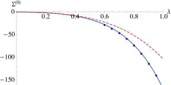
Figure 1: Plot of the function $\Sigma^{(0)}$ in (F.16), i.e. the planar contribution to $\langle\mathcal{W}^{2}\rangle_{\rm conn}$ (blue line). The red thin dashed line represents the contribution of the first two terms of the weak coupling expansion (F.8). The blue dots represent the leading term in the strong coupling expansion $-\frac{1}{8\pi\,\sqrt{2\lambda^{\prime}}}\,e^{2\pi\,\sqrt{2\lambda^{\prime}}}$, where $\lambda^{\prime}=\lambda-\frac{1}{24}$. The agreement is very good already at the moderate values of the coupling $\lambda\sim 1$.

Expressing $\kappa$ in terms of $\lambda$ using (F.13) we obtain for $\lambda\gg 1$

$$\langle\mathcal{W}^{2}\rangle =N^{2}\,(4\pi\lambda)^{-2}e^{2\pi\,\sqrt{2\lambda}}\,\Big{(}1+2\times\frac{2\pi^{2}\lambda^{2}}{3N^{2}}+\cdots\Big{)}+(2N)^{2}\frac{1}{N^{2}}\Big{(}-\frac{1}{32\pi\,\sqrt{2\lambda}}\,e^{2\pi\,\sqrt{2\lambda}}\Big{)}+\cdots$$

$$=W_{1}^{2}\Big{[}1+\frac{4\pi^{2}\lambda^{2}}{3N^{2}}-\frac{\sqrt{2}\pi\lambda^{3/2}}{N^{2}}+\mathcal{O}(N^{-4})\Big{]}\ ,$$ (F.19)

where $W_{1}$ is the leading-order planar strong coupling part in $\langle\mathcal{W}\rangle$ in (1.6),(E.4),(F.14). In terms of the dual string theory parameters in (1.2)) it reads

$$W_{1}=\frac{N}{4\pi\lambda}\,e^{\pi\,\sqrt{2\lambda}}=\frac{1}{\sqrt{2\pi}}\frac{\sqrt{T}}{g_{\text{s}}}\,e^{2\pi T}\ .$$ (F.20)

The leading correction $\frac{4\pi^{2}\lambda^{2}}{3N^{2}}=\frac{\pi}{6}\frac{g_{\text{s}}^{2}}{T}$ in (F.19) is just twice the correction in $\langle{\cal W}\rangle$ in (E.4),(1.6) corresponding to the factorized contribution $\langle\mathcal{W}\rangle^{2}$ while the connected contribution is thus subleading ($\lambda^{3/2}$ vs. $\lambda^{2}$) at large $\lambda$. We conclude that to leading order at strong coupling $\langle\mathcal{W}^{2}\rangle$ factorizes (cf. (1.19))

$$\langle\mathcal{W}^{2}\rangle=W_{1}^{2}\,\Big{(}1+\frac{\pi}{6}\,\frac{g_{\text{s}}^{2}}{T}+\cdots\Big{)}=\langle\mathcal{W}\rangle^{2}+...\ ,$$ (F.21)

i.e. the connected contribution (F.7) is subleading at large $\lambda\sim T^{2}$ at order $1/N^{2}\sim g^{2}_{\rm s}$.

It is tempting to conjecture that this factorization continues to be true also at higher orders in $1/N$ (as that happened in the SYM case for the fundamental – anti-fundamental Wilson loop correlator (4.55)). A test of this conjecture requires a much more involved calculation of $\Sigma^{(1)}$ term in (F.7) presented in the next subsection. Since $W_{1}^{2}\sim N^{2}$ this requires computing the $1/N^{4}\sim g^{4}_{\rm s}$ term in the brackets in (F.19).

F.2.1 $\langle\mathcal{W}^{2}\rangle$

The next to leading order correction to the two-point resolvent in (F.15) and thus to $\langle\mathcal{W}^{2}\rangle$ can be computed by working out the $1/N$ expansion of the loop equations of the ABJM matrix model (see, e.g., [14]). The exact result for $\Sigma^{(1)}$ in (F.16) valid for all values of the coupling $\alpha$ is quite involved

$$\Sigma^{(1)}=8\,\alpha^{2}\,\Big{[}-\frac{(a+b)^{2}(1+ab)^{2}(1+4ab+b^{2}+a^{2}(1+b^{2}))}{192a(-1+a^{2})^{2}b(-1+b^{2})^{2}}$$

$$+\frac{\mathbb{E}}{\mathbb{K}}\,\frac{1}{192a^{2}(-1+a^{2})^{4}b^{2}(-1+b^{2})^{4}}\Big{(}(1+ab)^{2}\big{[}b^{4}+b^{6}+a^{10}(b^{4}+b^{6})+3a^{2}b^{2}(6-7b^{2}-7b^{4}+6b^{6})$$

$$+3a^{8}b^{2}(6-7b^{2}-7b^{4}+6b^{6})+a^{4}(1+b^{2})(1-22b^{2}+44b^{4}-22b^{6}+b^{8})$$

$$+a^{6}(1+b^{2})(1-22b^{2}+44b^{4}-22b^{6}+b^{8})+2a(b+b^{3}-2b^{5}+b^{7}+b^{9})+2a^{9}(b+b^{3}-2b^{5}+b^{7}+b^{9})$$

$$+2a^{3}(b+12b^{3}-34b^{5}+12b^{7}+b^{9})+2a^{7}(b+12b^{3}-34b^{5}+12b^{7}+b^{9})$$

$$-4a^{5}(b+17b^{3}-42b^{5}+17b^{7}+b^{9})\big{]}\Big{)}+\Big{(}\frac{\mathbb{E}}{\mathbb{K}}\Big{)}^{2}\,\frac{1}{192a^{2}(-1+a^{2})^{4}b^{2}(-1+b^{2})^{4}}\Big{(}(1+ab)^{4}(a^{2}+a^{6}$$

$$-9a(-1+a^{2})^{2}(1+a^{2})b+(1-32a^{2}+54a^{4}-32a^{6}+a^{8})b^{2}+9a(-1+a^{2})^{2}(1+a^{2})b^{3}$$

$$+6a^{2}(9-16a^{2}+9a^{4})b^{4}+9a(-1+a^{2})^{2}(1+a^{2})b^{5}+(1-32a^{2}+54a^{4}-32a^{6}+a^{8})b^{6}$$

$$-9a(-1+a^{2})^{2}(1+a^{2})b^{7}+a^{2}(1+a^{4})b^{8})\Big{)}+\Big{(}\frac{\mathbb{E}}{\mathbb{K}}\Big{)}^{3}\,\frac{1}{192a^{2}(-1+a^{2})^{4}b^{2}(-1+b^{2})^{4}}\Big{(}-(1+ab)^{6}\big{[}5(b^{2}+b^{4})$$

$$+5a^{6}(b^{2}+b^{4})+4a^{3}b(3+4b^{2}+3b^{4})-4ab(4-3b^{2}+4b^{4})-4a^{5}b(4-3b^{2}+4b^{4})$$

$$+5a^{2}(1-2b^{2}-2b^{4}+b^{6})+5a^{4}(1-2b^{2}-2b^{4}+b^{6})\big{]}\Big{)}+\Big{(}\frac{\mathbb{E}}{\mathbb{K}}\Big{)}^{4}\,\frac{(a-b)^{2}(-1+ab)^{2}(1+ab)^{8}}{32a^{2}(-1+a^{2})^{4}b^{2}(-1+b^{2})^{4}}\Big{]}.$$ (F.22)

Expanded at weak coupling (F.2.1) is in agreement with (F.8). At strong coupling (i.e. large $\kappa$ in (F.10),(F.13)), we obtain for the leading term

$$\Sigma^{(1)}=-\frac{\kappa^{2}\,\log^{3}\kappa}{24\pi^{2}}+\cdots.$$ (F.23)

This gives an additional $1/N^{4}$ correction to the brackets in (F.19), i.e.

$$\langle\mathcal{W}^{2}\rangle=W_{1}^{2}\Big{[}1+{\cal O}\big{(}{1\over N^{2}}\big{)}-\frac{4\sqrt{2}\pi^{3}}{3}\frac{\lambda^{7/2}}{N^{4}}+...\Big{]}\ ,$$ (F.24)

which is indeed subleading compared to the similar term $(g_{\text{s}}^{2}/T)^{2}\sim{\lambda^{4}/N^{4}}$ in the square of $\langle\mathcal{W}\rangle$ in (E.4), i.e.

$$\langle\mathcal{W}\rangle^{2}=W_{1}^{2}\Big{[}1+{\pi\over 6}{g_{\text{s}}^{2}\over T}+{\pi^{2}\over 60}\Big{(}{g_{\text{s}}^{2}\over T}\Big{)}^{2}+...\Big{]}\ .$$ (F.25)

We conclude that there is no $(g_{\text{s}}^{2}/T)^{2}$ correction to (F.21), i.e. we have $\langle\mathcal{W}^{2}\rangle=\langle\mathcal{W}\rangle^{2}$ to this order.

F.2.2 $\langle\mathcal{W}^{3}\rangle$

It is interesting to consider also the first correction to the correlator $\langle\mathcal{W}^{3}\rangle$ of the three coincident Wilson loops at the leading order at strong coupling. $\langle\mathcal{W}^{3}\rangle$ may be again decomposed into factorized and connected contributions. From the usual scaling arguments, the $g_{\text{s}}^{2}/T$ correction may come only from $\langle\mathcal{W}\rangle^{3}$ and $\langle\mathcal{W}\rangle\langle\mathcal{W}^{2}\rangle_{\rm conn}$ while corrections to $\langle\mathcal{W}^{3}\rangle_{\rm conn}$ start at order $(g_{\text{s}}^{2}/T)^{2}$. From the above result (F.19) for $\langle\mathcal{W}^{2}\rangle$ (implying that $\langle\mathcal{W}^{2}\rangle_{\rm conn}$ is subleading) it follows that the $g_{\text{s}}^{2}/T$ term in $\langle\mathcal{W}^{3}\rangle$ is precisely three times that in $\langle\mathcal{W}\rangle$, i.e. comes only from $\langle\mathcal{W}\rangle^{3}$. At the next $(g_{\text{s}}^{2}/T)^{2}$ order we may have contribution only from $\langle\mathcal{W}^{3}\rangle_{\rm conn}$, since according to the result of the previous subsection there is no such leading term in $\langle\mathcal{W}^{2}\rangle_{\rm conn}$.

The weak coupling expansion of $\langle\mathcal{W}^{3}\rangle_{\rm conn}$ computed from the matrix model turns out to be

$$\langle\mathcal{W}^{3}\rangle_{\rm conn}=\frac{6}{N}\,\alpha^{2} +\Big{(}\frac{1}{2N}+\frac{9}{4N^{3}}\Big{)}\,\alpha^{4}+\Big{(}-\frac{27}{160N}-\frac{17}{96N^{3}}+\frac{81}{320N^{5}}\Big{)}\,\alpha^{6}$$

$$+\Big{(}-\frac{467}{13440N}+\frac{247}{3840N^{3}}-\frac{1}{960N^{5}}+\frac{243}{17920N^{7}}\Big{)}\,\alpha^{8}+\cdots$$ (F.26)

Hence, defining the coefficients in the $1/N$ expansion as (cf. (F.7))

$$\langle\mathcal{W}^{3}\rangle_{\rm conn}=\frac{1}{N}\,C^{(0)}+\frac{1}{N^{3}}\,C^{(1)}+\cdots,$$ (F.27)

we have

$$C^{(0)}=6\,\alpha^{2}+\frac{\alpha^{4}}{2}-\frac{27\,\alpha^{6}}{160}-\frac{467\,\alpha^{8}}{13440}+\cdots.$$ (F.28)

From the loop equations of the ABJM theory [14] we can determine the exact expression for the function $C^{(0)}$ by computing the planar three-point resolvent (cf. (F.15))

$$C^{(0)}=4\,\alpha\,\Big{[}\frac{(a+b)^{2}(1+ab)^{2}}{64a^{3}(-1+a^{2})^{2}b^{3}(-1+b^{2})^{2}}\Big{(}b-2b^{3}+b^{5}+a^{6}b(-1+b^{2})^{2}-a(1+b^{6})$$

$$\qquad\qquad\qquad\qquad+2a^{3}(1+b^{6})-a^{5}(1+b^{6})\Big{)}+\frac{(a-b)(-1+ab)(1+ab)^{6}}{32a^{2}(-1+a^{2})^{2}b^{2}(-1+b^{2})^{2}}\,\Big{(}\frac{\mathbb{E}}{\mathbb{K}}\Big{)}^{3}$$ (F.29)

$$-\frac{3(a-b)(-1+ab)(1+ab)^{4}\big{[}1+4ab+b^{2}+a^{2}(1+b^{2})\big{]}}{64a^{2}(-1+a^{2})^{2}b^{2}(-1+b^{2})^{2}}\,\Big{(}\frac{\mathbb{E}}{\mathbb{K}}\Big{)}^{2}+\frac{3(a-b)(a+b)^{2}(-1+ab)(1+ab)^{4}}{32a^{2}(-1+a^{2})^{2}b^{2}(-1+b^{2})^{2}}\,\frac{\mathbb{E}}{\mathbb{K}}\Big{]}.$$

This reproduces the weak coupling expansion (F.28). At strong coupling one finds

$$C^{(0)}=\frac{(3\log\kappa-1)(12\log^{2}\kappa+\pi^{2})}{384\,\pi\,\log^{3}\kappa}\,\kappa^{3}+\cdots\ \to\ \frac{3\kappa^{3}}{32\pi}+\cdots.$$ (F.30)

As a result,

$$\langle\mathcal{W}^{3}\rangle_{\rm conn} =\frac{1}{N}\frac{3}{32\pi}\,e^{3\pi\,\sqrt{2\lambda}}+\cdots=W_{1}^{3}\,\frac{6\pi^{2}\lambda^{3}}{N^{4}}+\cdots.$$ (F.31)

This contribution is subleading compared to the one $\sim W_{1}^{3}{g^{4}_{\rm s}\over T^{3}}\sim W_{1}^{3}{\lambda^{4}\over N^{4}}$ from factorized parts of the correlator $\langle\mathcal{W}^{3}\rangle$. We conclude that $\langle\mathcal{W}^{3}\rangle=\langle\mathcal{W}\rangle^{3}$ at order $(\frac{g_{\rm s}^{2}}{T})^{2}$, i.e. confirming (1.19).