Cumulative effects of collision integral, strong magnetic field, and quasiparticle description on charge and heat transport in thermal QCD medium

Abstract

Our first aim is to explore the effect of the collision integral with the insurance of instantaneous conservation of particle number on the charge and heat transport in a thermal QCD medium. The second aim is to see how the dimensional reduction due to strong magnetic field modulates the transport through the entangled effects such as the collision-time and occupation probability etc. in the collision integral. Final aim is to check how the quasiparticle description of partons, through the dispersion relation of thermal QCD in strong magnetic field, alters the aforesaid conclusions. We observe that the modified collision term expedites both transport, which is manifested by the larger magnitudes of electrical ($\sigma_{\rm el}$) and thermal ($\kappa$) conductivities, in comparison to the relaxation collision term. As a corollary, the Lorenz number is dominated by the later and the Knudsen number is by the former. However, the strong magnetic field not only flips the dominance of collision term in the heat transport, it also causes drastic enhancement of both $\sigma_{\rm el}$ and $\kappa$ and reduction in the specific heat. As a result, the equilibration factor, the Knudsen number becomes much larger than one, which defies physical interpretation. Finally, the quasiparticle description of partons in the absence of strong magnetic field impedes the transport of charge and heat, resulting in tiny decrease of the conductivities. However, the strong magnetic field does noticeable observations: the conductivities now gets reduced to the physically plausible values, the temperature dependence of $\sigma_{\rm el}$ gets reversed, i.e. it now decreases with temperature, effect of collision integral gets smeared in $\kappa$ etc. The Knudsen number thus becomes much smaller than one, implying that the system be remained in equilibrium. These findings attribute to the fact that the collective oscillation in the dispersion relation of thermal QCD in strong magnetic field sets in much larger scale, manifested by the large in-medium flavour masses.

1 Introduction

Quark Gluon Plasma (QGP), a deconfined state of quarks and gluons is formed in heavy ion collision experiments at Relativistic Heavy Ion collider (RHIC) and Large Hadron Collider (LHC). It is believed that our present universe was also in QGP form around one microsecond after the big bang. There exists such hot and dense matter in the core of the neutron stars also. In the ongoing heavy ion collision experiments at RHIC and LHC, a very strong magnetic field, perpendicular to the reaction plane, could be produced in the very early stages of the collisions in noncentral events[1, 2] viz. order of $m_{\pi}^{2}$ at RHIC [3] and $15m_{\pi}^{2}$ at LHC [4]. Some very naive estimates predict that the decay of the magnetic field in the non-conducting medium is very fast but due to the finite value of the electrical conductivity of the medium, the decay time for the magnetic field gets elongated, which may then cause to affect the physical quantities associated with QGP. In the recent years, the effects of the background magnetic field on the various properties of the QGP have been investigated by the various research groups, such as the chiral magnetic effect[5, 3], magnetic and inverse magnetic catalysis[6, 7, 8, 9], axial magnetic effect[10, 11], chiral vortical effect in rotating QGP [12, 13], the conformal anomaly and production of soft photons[14, 15], apart from that the dilepton production rate[16, 17, 18], dispersion relation in the magnetized thermal QED[19], refractive indices and decay constants[20, 14] and various thermodynamical properties [21, 22].

In the strong magnetic field ($|q_{i}B|>>T^{2}$ and $|q_{i}B|>>m^{2}_{i}$, where $q_{i}(m_{i})$ is the electric charge (mass) of the $i$-th flavour), the dynamics of charged particles are constrained only in the lowest Landau levels, so the dispersion relation ($E=\sqrt{p_{3}^{2}+m_{i}^{2}}$, involves only the momentum ($p_{3}$) along the direction of magnetic field. Some recent observations [23, 24] indicates the similarity of the time scales between the formation of the locally equilibrated thermal QCD medium and the production of strong magnetic field, due to faster thermalization. Thus, the transport properties of the medium may be affected due to presence of the strong magnetic field. Electrical conductivity $(\sigma_{el})$, which is responsible for the generation of electric current due to Lenz’s law plays a vital role in the study of the chiral magnetic effect [5]. Apart from that, $\sigma_{el}$ plays very crucial role as an input parameter in the phenomenological studies at RHIC and LHC, such as the emission rate of soft photons [25]. The effect of the magnetic field on the electrical conductivity has been previously studied using different approaches, such as the dilute instanton-liquid model [26], the nonlinear electromagnetic currents [27, 28], the diagrammatic method using real time formalism [29], quenched SU(2) lattice gauge theory [30], axial Hall current [31], the effective fugacity approach [32] etc.

Another important transport coefficient is the thermal conductivity ($\kappa$), which is the measure of a medium to conduct the heat through it. The thermal dissipation in the medium depends on the temperature gradient associated with the different layers of the fluid. The studies on $\kappa$ of the hot QCD matter in a strong magnetic field have recently been done in  [33, 34]. In fact, $\kappa$ plays a crucial role in terms of Knudsen number to check that the system is in local equilibrium. The Knudsen number is the ratio of the mean free path $(\lambda)$ to the characteristic length of the system ($L$), where $\lambda$ is related to $\kappa$ by $\lambda=3\kappa/({\mathrm{v}C_{V}})$ (where ${\rm v}$ is the relative velocity of quark and ${\mathrm{C}_{V}}$ is the specific heat at the constant volume). The system is said to be in local hydrodynamic equilibrium if the mean free path is smaller than the characteristic length of the medium. The $\sigma_{{\rm el}}$ and $\kappa$ are not independent rather their ratio $\kappa/\sigma_{el}$ is equal to the product of Lorentz number $L_{R}$ and the temperature, this relation is commonly known as the Wiedemann-Franz Law. Metals being good conductor of heat and electricity follow Wiedemann-Franz law perfectly. However, violation of the this law has been recorded in many systems such as, the two-flavor quark matter in the Nambu-Jona-lasinio model [35], the strongly interacting QGP medium [36], thermally populated electron-hole plasma in graphene [37] the unitary Fermi gas [38, 39] and the hot hadronic matter [40].

In the previous studies [34, 41], the transport coefficients have been calculated from the Boltzmann equation and the complexities of the collision term was avoided by a mean-free-path treatment. In this treatment, the collision integral is simplified by a relaxation term, implying that the collisions tend to relax the distribution function to an equilibrium value. The relaxation model then describes the destruction of phase of an ordered motion on collision and leads to a damping frequency of order $1/\tau$ in the amplitude, where $\tau$ is some suitable average collision time. This type of model has a flaw that charge is not conserved instantaneously but only on the average over a cycle. It is, however, easy to remedy this at least in the case of constant collision time by modifying the collision term due to Bhatnagar-Gross-Krook (BGK) [42]. The BGK collision term differs physically from the relaxation type in the following manner: Each collision term in a Boltzmann equation consists of two parts, where the first one represents particles removed or absorbed from a definite momentum range by collisions and the second one represents the particles emitted into that range as a result of collisions. The absorption term is essentially the same as that in the relaxation term, i.e. particles in a momentum range $d\vec{p}$ about the momentum $\vec{p}$ are absorbed at a rate proportional to perturbed distribution $f(\vec{x},\vec{p},t)$. The emission term is the real source of difficulty, for which BGK prescribed that particles emitted at a rate proportional to the product of perturbed particle density, $n(\vec{x},t)$ and the equilibrium distribution function [42]. The effect of the BGK collision term which ensures the conservation of the particle number instantaneously has been studied on the plasma instabilities in  [43].

Thus, the aim of the present work is to extend/modify of the aforesaid recent works[34] on the transport of charge and heat in a hot quark matter in three fold respects: (i) By modifying the collision terms as mentioned above, the solution of Boltzmann equation for the infinitesimal disturbance gets altered, which, in turn, affects the transport coefficients directly. (ii) The effect of a strong magnetic field, a possibility in the peripheral events of ultrarelativistic heavy-ion collisions, is explored, due to the reduction of phase space and the enhancement of the collision time etc. (iii) Finally the role of interactions is explored in the quasiparticle description of partons, where the vacuum masses of partons are replaced by the masses generated in the medium. These masses are obtained from the pole of full propagator, calculated by the perturbative thermal QCD in the background of strong magnetic field. Thus, we have employed a kinetic theory approach with the BGK Collision term in Boltzmann equation to compute the electrical ($\sigma_{el}$) and thermal ($\kappa$) conductivities and the derived coefficients (Lorenz and Knudsen number) from them.

We have found that the modified collision integral enhances the magnitudes of both conductivities, especially more to the electrical conductivity, compared to the counter-parts with the collision term of relaxation type. As a consequence, the ratio, $\kappa/\sigma_{\rm el}$ and the Lorenz number, $L_{R}$ $(=\kappa/\sigma_{el}T)$ gets decreased whereas the the equilibration factor, Knudsen number gets increased. In the presence of strong magnetic field, interesting thing happens in the transport. Although there is an overall enhancement of both conductivities but $\kappa$ becomes smaller than in relaxation collision integral. This could be attributed to the constrained motion of quarks in strong magnetic field. As a corollary, the Knudsen number becomes much larger than one, due to the enhancement of $\kappa$ and the reduction of specific heat, thus necessitates the quasiparticle description (QPD) of partons for the transport phenomena, at least, in strong $B$. In fact, the QPD of partons (mainly for quarks) in the absence of magnetic field makes the transport coefficients a little bit smaller but in the presence of strong magnetic field, QPD enriches the transport phenomena interesting: $\sigma_{el}$ now decreases with temperature and $\kappa$ becomes insensitive to the collision integral, except the temperature is very high. As a result, the Knudsen number does not depend on the type of collision integral and becomes much smaller than one, which ensures that the system is still in local equilibrium even in the presence of strong $B$. This could be envisaged by the fact that the collective oscillation of a thermal QCD medium in strong $B$ sets in much bigger scale than in the absence of magnetic field.

The paper has been organized as follows: In section 2, we have investigated the effect of the collision term via the collision integral and the effect of (strong) magnetic field on the charge and heat transport, separately, in a thermal medium of noninteracting quarks and gluons. For that purpose, we have employed the kinetic theory approach through the relativistic Boltzmann transport equation. In particular, subsections 2.1 and 2.2 deal with the charge and heat transport via the computation of electrical and thermal conductivities, respectively. The subsection 2.3 explores the transport coefficients related the competition between thermal and charge transport through the ratio, $\kappa/\sigma_{el}$ (and the Lorenz number, $L_{R}$ in Wiedemann-Franz Law) and the validity of local equilibration through the Knudsen number. Thus, having explored the sole effect of collision terms on the charge and heat transport, we explore the sole effect of background strong magnetic field on the aforesaid transport coefficients in subsections 2.4 and 2.5, respectively. We have found that the magnitude of conductivities for noninteracting partons in strong magnetic field defy physical interpretation, contrary to the spirit of the linearization of the collision integral on the basis of near-equilibrium assumption. This motivates us to compute the same in section 3 with the interactions present among the constituents of the medium in the guise of quasiparticle description of partons. So we have first revisited the medium generated thermal masses for the quark flavors in the presence of the strong magnetic field in subsection 3.1 and then investigate how the quasiparticle description in section 3.1 affects the abovementioned transport phenomena and found the plausible magnitudes of the conductivities and other derived transport coefficients. Finally Section 4 concludes results and discussions.

2 Charge and Heat Transport in a thermal medium of noninteracting quarks and gluons

The Boltzmann transport equation for a single particle distribution function is given by

$$\frac{\partial f}{\partial t}+\frac{\mathbf{p}}{m}\cdot\nabla f+{\mathbf{F}}\cdot\frac{\partial f}{\partial\mathbf{p}}={\left(\frac{\partial f}{\partial t}\right)}_{\rm coll},$$ (1)

where ${\mathbf{F}}$ is the force field acting on the particles in the medium and the term on the right hand side is added to describe the effect of collisions between particles. If the collision term is zero then the particles do not collide, where individual collisions get replaced with long-range aggregated Coulomb interactions, referred as the collisionless Boltzmann equation or Vlasov equation.

The solution of the Boltzmann equation is, in general, a matter of considerable difficulty even in the cases corresponding to the physically simplest situations. The main difficulty in handling the full Boltzmann equation arises from the complicated nature of the collision terms, consisting of absorption and emission terms. The absorption causes the removal of particles from a definite momentum range by collisions and then the particles are emitted into that range as a result of collisions. The absorption term is substantially the same as that in the Boltzmann equation, i.e. particles in a momentum range $d\vec{p}$ about the momentum $\vec{p}$ are absorbed at a rate proportional to perturbed distribution $f(\vec{x},\vec{p},t)$. The emission term is the real source of difficulty for which we will now discuss some simple kinetic models, which permit of exact mathematical treatment including the solution of definite boundary value problems.

In many kinetic problems, it is convenient to avoid the complexities of the Boltzmann equation by using a mean free-path treatment, where one replaces the collision integral by a relaxation term of the form

$${\left(\frac{\partial f}{\partial t}\right)}_{\rm coll}=-\frac{1}{\tau(p)}\left(f(\vec{x},\vec{p},t)-f_{\rm eq}(|\vec{p}|)\right),$$ (2)

where $\tau$ is the momentum-dependent collision time, which implies that the collisions tend to relax the distribution function to an equilibrium value $f_{\rm eq}(|\vec{p}|)$, which is a function of momentum only. We illustrate the collision models by referring to oscillatory problems, where a characteristic time enters in a natural way. The above collision term (2) of relaxation type then describes the destruction of phase of an ordered motion on collision and leads to a damping frequency of order $1/\tau$ in the amplitude, where $\tau$ is some suitable average collision time. This type of model has the defect that the charge is not conserved instantaneously but only on the average over a cycle. It was first remedied by Bhatnagar-Gross-Krook (BGK) [42] , where the particles in a range $d^{3}p$ about momentum $\vec{p}$ are absorbed at a rate proportional to the number $f(\vec{p},\vec{x},t)$ at $(\vec{x},t)$, and are re-emitted at a rate proportional to the perturbed density, $n(\vec{x},t)$ (=$\int f(\vec{x},\vec{p},t)d^{3}p$). The BGK collision term is given by [43, 42]

$${\left(\frac{\partial f}{\partial t}\right)}_{\rm coll}=-\frac{1}{\tau}\left(f(\vec{x},\vec{p},t)-\frac{n(\vec{x},t)}{n_{\mathrm{e}q}}f_{\rm eq}(|\vec{p}|)\right),$$ (3)

which upon integrating over momenta vanishes i.e. it conserves the particle number instantaneously. Its effect was extensively discussed on QCD plasma instabilities [43].

Till now we have discussed the nonrelativistic version of the Boltzman equation, however, the transport phenomena for a medium consisting of quarks and gluons could be better understood by the relativistic generalization of Boltzmann equation, which is oftenly expressed in a covariant form as

$$p^{\mu}\frac{\partial f}{\partial x^{\mu}}+q~{}F^{\rho\sigma}p_{\sigma}\frac{\partial f}{\partial p^{\rho}}=-\frac{p^{\mu}u_{\mu}}{\tau}\left(f(\vec{x},\vec{p},t)-\frac{n(\vec{x},t)}{n_{\mathrm{e}q}}f_{\rm eq}(|\vec{p}|)\right),$$ (4)

where $F^{\mu\nu}$ is the external electromagnetic force. We will now see in forthcoming sections how the abovementioned collision integral affects the solution of the relativistic Boltzman equation, which, in turn, alters the transport of electricity and heat in terms of their respective transport coefficients, such as the electrical and thermal conductivities and the derived coefficients from them, namely Lorenz and Knudsen number. Furthermore we also explore how a strong magnetic field could modulate the effect of modified collision term on the aforesaid transport processes.

2.1 Electrical conductivity in the absence of magnetic field

The linear response of a medium consisting of mobile charge carriers to an infinitesimal electric field (${\bf E}$) deciphers the electrical properties of the medium. The electric field induces a current ($\vec{J}$) in the medium, which is proportional linearly to the (infinitesimal) applied ${\bf E}$ and the proportionality constant, known as the electrical conductivity ($\sigma_{\rm el}$), determines the electrical properties of the given medium. For a thermal QCD medium consisting of quarks, antiquarks and gluons of different flavours ($i$), the four-component induced current, contributed by quarks and antiquarks only, becomes

$$J_{\mu}=\sum_{i}q_{i}g_{i}\int\frac{d^{3}p}{(2\pi)^{3}}~{}\frac{p_{\mu}}{\omega_{i}}~{}(\delta f_{i}(x,p)+\delta\bar{f}_{i}(x,p))$$ (5)

where, $q_{i},$ $g_{i}$ and $\delta f_{i}(x,p)$ are the charge, degeneracy factor and the infinitesimal deviation from the equilibrium distribution function for ${\rm i}$-th quark, respectively. Similarly $\delta\bar{f}_{i}(x,p)$ denotes for ${\rm i}$-th anti-quarks, which, for vanishingly small quark chemical potential ($\mu\approx 0$), is the same as for quarks, $\delta f_{i}(x,p)$. Therefore, the induced current can be calculated provided the infinitesimal deviation, $\delta f_{i}$ is known. In kinetic theory approach, the $\delta f_{i}$ is obtained from the solution of relativistic Boltzman equation, after linearizing the collision integral with respect to a (infinitesimal) perturbation to a medium, which was initially in equilibrium.

In order to see the responce of the electric field, we take only $\rho=i$ and $\sigma=0$ and vise versa components of the electromagnetic field strength tensor, i.e. $F^{0i}=-{\bf E}$ and $F^{i0}={\bf E}$ in the relativistic Boltzman equation (RTBE) in (4). Hence, the RTBE (4) gets reduced for the $i$-th species in a multicomponent medium

$$q_{i}{\bf E.p}\frac{\partial f_{i}}{\partial p^{0}}+q_{i}p_{0}{\bf E.}\frac{\partial f_{i}}{\partial{\bf p}}=C[f].$$ (6)

The modified collision integral $C[f]$ in (6) due to BGK is generalized for the $i$-th species of a multicomponent system as

$$C[f]=-p^{\mu}u_{\mu}\nu_{i}\left(f_{i}-n_{{}_{i}}n_{\mathrm{e}q,i}^{-1}f_{\mathrm{e}q,i}\right),$$ (7)

where $f_{\mathrm{e}q,i}$ is the equilibrium distribution function of $i$-th flavour:

$$f_{\mathrm{e}q,i}=\frac{1}{e^{\beta u^{\alpha}{p_{\rm i}}_{\alpha}}+1},$$ (8)

where $p_{\rm i}^{\alpha}$ is $(\omega_{i},\vec{p})$ and $u_{\alpha}$ is the fluid four-velocity, which, in the local rest frame, is $u_{\mu}=(1,0,0,0)$. The collision frequency, $\nu_{i}$ is the inverse of the relaxation-time of the medium, $\tau_{i}$. The relaxation time can also be calculated from the Boltzmann equation, where the gluon-gluon collision mainly plays the dominant role in the collision integral, to bring the perturbed system back to the equilibrium. The expression for $\tau$ is given by [44]

$$\tau_{i}(T)=\frac{1}{5.1T\alpha_{s}^{2}\log(\frac{1}{\alpha_{s}})[1+0.12(2N_{i}+1)]},$$ (9)

where $\alpha_{s}$ is the running coupling constant, which runs with the temperature as

$$\alpha_{s}(T)=\frac{6\pi}{(33-2N_{f})\ln(\frac{Q}{\Lambda_{QCD}})},$$ (10)

where $Q$ is set at $2\pi T$.

The symbol, $n_{i}$ in the above collision integral (7) represents the perturbed density for $i$-th species

$$n_{i} = g_{i}\int\frac{d^{3}p}{(2\pi)^{3}}(f_{\mathrm{e}q,i}+\delta f_{i}),$$ (11)

and the equilibrium density for $i$-th flavour, having degeneracy factor, $g_{i}$, is given by

$$n_{\mathrm{e}q,i}=g_{i}\int\frac{d^{3}p}{(2\pi)^{3}}f_{\mathrm{e}q,i}.$$ (12)

After linearizing the collision integral with respect to the infinitesimal perturbation: $f_{\mathrm{e}q,i}\rightarrow f_{\mathrm{e}q,i}+\delta f_{i},~{}\delta f_{i}\ll f_{\mathrm{e}q,i}$, the RTBE (6) is recast into the form (Details are given in Appendix A)

$$\delta f_{i}-g_{i}n_{\mathrm{e}q,i}^{-1}f_{\mathrm{e}q,i}\int_{p}\delta f_{i}=2q_{i}\beta\tau_{i}~{}\frac{{\bf E\cdot p}}{\omega_{i}}f_{\mathrm{e}q,i}\left(1-f_{\mathrm{e}q,i}\right),$$ (13)

wherein the following partial derivatives have been used:

$$\frac{\partial f_{\mathrm{e}q,i}}{\partial p^{0}} = -\beta f_{\mathrm{e}q,i}(1-f_{\mathrm{e}q,i}),$$ (14)

$$\frac{\partial f_{\mathrm{e}q,i}}{\partial{\bf p}} = -\frac{\beta{\bf p}}{\omega_{i}}f_{\mathrm{e}q,i}(1-f_{\mathrm{e}q,i}).$$ (15)

Therefore, the solution for $\delta f_{i}$ is obtained (neglecting the higher order, ${\cal O}{(\delta f_{i})}^{2}$) as

$$\delta f_{i}=\delta f_{i}^{(0)}+g_{i}n_{\mathrm{e}q,i}^{-1}f_{\rm eq,i}\int_{p^{\prime}}\delta f_{i}^{(0)},$$ (16)

where

$$\delta f_{i}^{(0)}=\frac{2\beta q_{i}\tau_{i}}{\omega_{i}}{\bf E.p}~{}f_{\mathrm{e}q,i}(1-f_{\mathrm{e}q,i}).$$ (17)

Thus, the spatial component of the four-vector for the induced current is finally obtained by plugging $\delta f_{i}$ into (5),

$$J_{k} = 4\beta\sum_{i}q_{i}^{2}g_{i}\tau_{i}\left[\int\frac{d^{3}p}{(2\pi)^{3}}~{}\frac{p_{k}^{2}}{\omega_{i}^{2}(p)}f_{\mathrm{e}q,i}(p)(1-f_{\mathrm{e}q,i}(p))\right.$$ (18)

$$\left.+g_{i}n_{\mathrm{e}q,i}^{-1}\int_{p}~{}\frac{p_{k}}{\omega_{i}(p)}f_{\mathrm{e}q,i}(p)\int_{p^{\prime}}\frac{p^{\prime}_{k}}{\omega_{i}(p^{\prime})}f_{\mathrm{e}q,i}(p^{\prime})(1-f_{\mathrm{e}q,i}(p^{\prime}))\right]E_{k}.$$

Hence, the coefficient of ${\bf E}$ in the above induced current, ${\bf J}$ thus yields the electrical conductivity in the modified collision term which can be decomposed in terms of the contribution due to the collision term of the relaxation type (2) and a correction term as

$$\sigma_{\rm el}=\sigma_{\rm el}^{\rm RT}+\sigma_{\rm el}^{\rm Corr},$$ (19)

where

$$\sigma_{\rm el}^{\rm RT} = 4\beta\sum_{i}q_{i}^{2}g_{i}\tau_{i}\int_{p}~{}\frac{p^{2}}{3\omega_{i}^{2}(p)}f_{\mathrm{e}q,i}(p)(1-f_{\mathrm{e}q,i}(p)),$$ (20)

$$\sigma_{\rm el}^{\rm Corr} = 4\beta\sum_{i}q_{i}^{2}g^{2}_{i}\tau_{i}n_{\mathrm{e}q,i}^{-1}\int_{p}~{}\frac{p}{\omega_{i}}f_{\mathrm{e}q,i}(p)\int_{p^{\prime}}\frac{d^{3}p^{\prime}}{(2\pi)^{3}}\frac{p^{\prime}}{\omega_{i}(p^{\prime})}f_{\mathrm{e}q,i}(p^{\prime})(1-f_{\mathrm{e}q,i}(p^{\prime})),$$ (21)

where $\sigma_{\rm el}^{\rm Corr}$ is found to be positive, implying that the modified BGK collision term always enhances the charge transport.

2.2 Thermal conductivity in the absence of magnetic field

In this section, we will calculate the thermal conductivity from the surplus of the energy diffusion over the enthalpy diffusion, known as the heat flow. In four-vector notation, the heat-flow is defined as

$$Q_{\mu}=\Delta_{\mu\alpha}T^{\alpha\beta}u_{\beta}-h\Delta_{\mu\alpha}N^{\alpha},$$ (22)

where the projection tensor, $\Delta_{\mu\alpha}$ is given by

$$\Delta_{\mu\alpha}=g_{\mu\alpha}-u_{\mu}u_{\alpha},$$ (23)

and the enthalpy per particle, $h$ is

$$h=(\varepsilon+P)/n,$$ (24)

where $\varepsilon$, $P$, and $n$ are the energy, pressure, and particle number densities, respectively. $N^{\alpha}$ and $T^{\alpha\beta}$ are the particle flow number and the energy-momentum tensor (also known as the first and second moment of the distribution function, respectively), respectively, and are defined in the kinetic theory for a multi-component system as

$$N^{\alpha} = \sum_{i}2g_{i}\int\frac{d^{3}p}{(2\pi)^{3}}~{}\frac{p^{\alpha}}{\omega_{i}}~{}f_{\mathrm{e}q,i},$$ (25)

$$T^{\alpha\beta} = \sum_{i}2g_{i}\int\frac{d^{3}p}{(2\pi)^{3}}\frac{p^{\alpha}p^{\beta}}{\omega_{i}}~{}f_{\mathrm{e}q,i},$$ (26)

which yield $n$, $\varepsilon$ and $P$ by the following contractions:

$$n = N^{\alpha}u_{\alpha},$$ (27)

$$\varepsilon = u_{\alpha}T^{\alpha\beta}u_{\beta},$$ (28)

$$P = -\frac{\Delta_{\alpha\beta}T^{\alpha\beta}}{3},$$ (29)

respectively.

In the rest frame of the fluid, the heat flow four vector is orthogonal to the fluid four-velocity

$$Q^{\mu}u_{\mu}=0,$$ (30)

so, both temporal and spatial components are not independent rather the heat four vector can be determined by its spatial component alone. Thus, the spatial component is read off from (22) and can be expressed in kinetic theory for a multi-component system as

$${\bf Q}=\sum_{i}2g_{i}\int\frac{d^{3}p}{(2\pi)^{3}}~{}\frac{\bf p}{\omega_{i}}~{}(\omega_{i}-h_{i})~{}\delta f_{i},$$ (31)

where, the enthalpy per particle for the $i^{th}$ flavour is,

$$h_{i} = \frac{(\epsilon_{i}+P_{i})}{n_{\mathrm{e}q,i}}$$ (32)

with

$$\epsilon_{i} = g_{i}\int\frac{d^{3}p}{(2\pi)^{3}}\omega_{i}f_{\mathrm{e}q,i}$$ (33)

$$P_{i} = \frac{g_{i}}{3}\int\frac{d^{3}p}{(2\pi)^{3}}\frac{p^{2}}{\omega_{i}}f_{\mathrm{e}q,i}$$ (34)

respectively.

In order to understand the dissipative processes in a medium in kinetic theory approach, namely the thermal conduction and viscosity etc., one usually goes to the next approximation beyond the initial local equilibrium distribution function: $f_{i}=f_{\mathrm{e}q,i}+\delta f_{i}$ ($\delta f_{i}$ $\ll f_{\mathrm{e}q,i}$) and $\delta f_{i}$ is thereafter obtained from the Boltzmann equation (4), after linearizing the collision integral with respect to the deviation.

So we start with rewriting the RTBE (4) in a suitable form through the chain rule of differentiation

$$p^{\mu}\frac{\partial f_{i}}{\partial T}\frac{\partial T}{\partial x^{\mu}}+p^{\mu}\frac{\partial f_{i}}{\partial p^{0}}\frac{\partial(p^{\nu}u_{\nu})}{\partial x^{\mu}}+q_{i}\left[F^{0j}{\bf p}\frac{\partial f_{i}}{\partial p^{0}}+F^{j0}p_{0}\frac{\partial f_{i}}{\partial p^{j}}\right]=C[f].$$ (35)

Now, going beyond the initial local equilibrium distribution function, we first compute the left hand side of RTBE (35) as

$${\rm LHS} = (p^{0}\partial_{0}T+p^{j}\partial_{j}T)\frac{\partial f_{\mathrm{e}q,i}}{\partial T}+(p^{\mu}u_{\nu}\partial_{\mu}p^{\nu}+p^{\mu}p^{\nu}\partial_{\mu}u_{\nu})\frac{\partial f_{\mathrm{e}q,i}}{\partial p^{0}}+q_{i}\left[{\bf E.p}\frac{\partial f_{\mathrm{e}q,i}}{\partial p^{0}}+{\bf E}p_{0}\frac{\partial f_{\mathrm{e}q,i}}{\partial p^{j}}\right],$$ (36)

$$= \frac{p^{0}}{T}f_{\rm eq,i}(1-f_{\rm eq,i})\left[\frac{1}{T}(p^{0}\partial_{0}T+p^{j}\partial_{j}T)-\frac{1}{p^{0}}(p^{\mu}u_{\nu}\partial_{\mu}p^{\nu}+p^{\mu}p^{\nu}\partial_{\mu}u_{\nu})-2q_{i}\frac{{\bf E.p}}{p^{0}}\right],$$

$$= \frac{p^{0}}{T}f_{\rm eq,i}(1-f_{\rm eq,i})\left[\frac{1}{T}(p^{0}\partial_{0}T+p^{j}\partial_{j}T)-\frac{1}{p^{0}}(p^{0}\partial_{0}p^{0}+p^{j}\partial_{j}p^{0})-\frac{1}{p^{0}}(p^{0}p^{\nu}\partial_{0}u_{\nu}+p^{j}p^{\nu}\partial_{j}u_{\nu})\right.$$

$$\left.-2q_{i}\frac{{\bf E.p}}{p^{0}}\right]$$

$$= \frac{p^{0}}{T}f_{\rm eq,i}(1-f_{\rm eq,i})\left[\frac{1}{T}(p^{0}\partial_{0}T+p^{j}\partial_{j}T)+T\partial_{0}\left(\frac{\mu}{T}\right)+\frac{T}{p^{0}}p^{j}\partial_{j}\left(\frac{\mu}{T}\right)-\frac{1}{p^{0}}(p^{0}p^{\nu}\partial_{0}u_{\nu}+p^{j}p^{\nu}\partial_{j}u_{\nu})\right.$$

$$\left.-\frac{2q_{i}{\bf E.p}}{p^{0}}\right].$$

The energy-momentum conservation facilitates to calculate the partial derivatives appeared in the above equation as

$$\partial_{j}\left(\frac{\mu_{i}}{T}\right) = -\frac{h_{i}}{T^{2}}\left(\partial_{j}T-\frac{T}{n_{\mathrm{e}q,i}h_{i}}\partial_{j}P\right)$$ (37)

$$\partial_{0}u_{\nu} = \frac{\nabla_{\nu}P}{n_{\mathrm{e}q,i}h_{i}}.$$ (38)

Thus, the RTBE (35) is written by linearizing the BGK collision term (7)

$$\frac{p^{0}}{T}f_{\rm eq,i}(1-f_{\rm eq,i})\left[\frac{p^{0}}{T}\partial_{0}T+\frac{(p^{0}-h_{i})}{p^{0}}\frac{p^{j}}{T}\left(\partial_{j}T-\frac{T}{n_{\mathrm{e}q,i}h_{i}}\partial_{j}P\right)+T\partial_{0}\left(\frac{\mu_{i}}{T}\right)-\frac{p^{j}p^{\nu}}{p^{0}}\partial_{j}u_{\nu}\right.$$

$$\left.-2q_{i}\frac{{\bf E.p}}{p^{0}}\right]=-p^{\mu}u_{\mu}\nu_{i}\left(\delta f_{i}-g_{i}n_{\mathrm{e}q,i}^{-1}f_{\rm eq,i}\int_{p}\delta f_{i}\right),$$ (39)

which is further solved to obtain $\delta f_{i}$ (neglecting its higher orders)

$$\delta f_{i}=\delta f_{i}^{(1)}+g_{i}n_{\mathrm{e}q,i}^{-1}f_{\rm eq,i}\int_{p^{\prime}}\delta f_{i}^{(1)},$$ (40)

where

$$\delta f_{i}^{(1)} = -\frac{f_{\rm eq,i}(1-f_{\rm eq,i})\tau_{i}}{T}\left[\frac{p^{0}}{T}\partial_{0}T+\frac{(p^{0}-h_{i})}{p^{0}}\frac{p^{j}}{T}\left(\partial_{j}T-\frac{T}{n_{\mathrm{e}q,i}h_{i}}\partial_{j}P\right)+T\partial_{0}\left(\frac{\mu_{i}}{T}\right)\right.$$ (41)

$$\left.-\frac{p^{j}p^{\nu}}{p^{0}}\partial_{j}u_{\nu}-2q_{i}\frac{{\bf E.p}}{p^{0}}\right].$$

Thus, the spatial part of the heat flow vector is obtained by plugging $\delta f_{i}$ into the equation (31).

$${Q_{j}} = \sum_{i}2g_{i}\int\frac{{d^{3}p}}{(2\pi)^{3}}~{}\frac{{p_{j}}}{\omega_{i}(p)}~{}(\omega_{i}(p)-h_{i})\left[\left\{\frac{f_{\mathrm{e}q,i}(p)(1-f_{\mathrm{e}q,i}(p))\tau_{i}}{T}\frac{(p^{0}-h_{i})}{p^{0}}\frac{p_{j}}{T}\right.\right.$$ (42)

$$\left.\left.+g_{i}n_{\mathrm{e}q,i}^{-1}f_{\mathrm{e}q,i}(p)\int_{p^{\prime}}\frac{f_{\mathrm{e}q,i}(p^{\prime})(1-f_{\mathrm{e}q,i}(p^{\prime}))\tau_{i}}{T}\frac{(p^{0}-h_{i})}{p^{0}}\frac{p_{j}}{T}\right\}\left(\partial_{j}T-\frac{T}{nh_{i}}\partial_{j}P\right)\right.$$

$$\left.+\left(\frac{f_{\mathrm{e}q,i}(p)(1-f_{\mathrm{e}q,i}(p))\tau_{i}}{T}+g_{i}n_{\mathrm{e}q,i}^{-1}f_{\mathrm{e}q,i}(p)\int_{p^{\prime}}\frac{f_{\mathrm{e}q,i}(p^{\prime})(1-f_{\mathrm{e}q,i}(p^{\prime}))\tau_{i}}{T}\right)\left\{\frac{p^{0}}{T}\partial_{0}T+T\partial_{0}\left(\frac{\mu}{T}\right)\right.\right.$$

$$\left.\left.-\frac{p^{j}p^{\nu}}{p^{0}}\partial_{j}u_{\nu}-2q_{i}\frac{{\bf E\cdot p}}{p^{0}}\right\}\right].$$

In order to define the thermal conductivity for a system, the number of particles in that system must be conserved and therefore it requires the associated chemical potential to be nonzero. In the ultrarelativistic heavy-ion collisions at RHIC and LHC, the value of chemical potential $(\mu)$ is very small [45, 46, 47], its value extracted from the charged particle ratios are in the range of 50-100 MeV. In Navier-Stokes equation, the heat flow vector is related to the gradient of the thermal potential, $U_{i}=\mu_{i}/T$ as

$$Q^{i}_{\mu} \stackrel{{\scriptstyle\rm Def}}{{=}} -\kappa\frac{n_{\mathrm{e}q,i}}{\epsilon_{i}+P_{i}}T^{2}\nabla_{\mu}U_{i},$$ (43)

$$= \kappa\left[\nabla_{\mu}T-\frac{T}{\epsilon_{i}+P_{i}}\nabla_{\mu}P_{i}\right],$$

where the coefficient, $\kappa$ is the thermal conductivity and $\nabla_{\mu}=\partial_{\mu}-u_{\mu}u_{\nu}\partial^{\nu}$. In the local rest frame of the fluid, only the spatial ($j$) component of the heat flow four vector for $i$-th species is retained and takes the form

$${Q^{i}_{j}} = -\kappa\left[\frac{\partial T}{\partial x_{j}}-\frac{T}{n_{\mathrm{e}q,i}h_{i}}\frac{\partial P_{i}}{\partial{x_{j}}}\right].$$ (44)

Thus, we have obtained the thermal conductivity by comparing the heat flow (${\mathbf{Q}}$) calculated from the kinetic theory (42) with its definition (44). The effect of the modified collision term on the thermal conductivity can be decomposed in terms of the contribution due to the collision term of the relaxation type (RT) and a correction term as,

$$\kappa = \kappa^{\rm RT}+\kappa^{\rm Corr},$$ (45)

where

$$\kappa^{\rm RT} = \beta^{2}\sum_{i}2g_{i}\tau_{i}\left[\int_{p}\frac{p^{2}}{3\omega_{i}^{2}(p)}(\omega_{i}(p)-h_{i})^{2}f_{\rm eq,i}(p)(1-f_{\rm eq,i}(p))\right].$$ (46)

$$\kappa^{\rm Corr} = \beta^{2}\sum_{i}2g^{2}_{i}\tau_{i}n_{\mathrm{e}q,i}^{-1}\int_{p}\frac{p}{\omega_{i}(p)}(\omega_{i}(p)-h_{i})f_{\rm eq,i}(p)$$ (47)

$$\times\int_{p^{\prime}}\frac{p^{\prime}}{\omega_{i}(p^{\prime})}(\omega_{i}(p^{\prime})-h_{i})f_{\rm eq,i}(p^{\prime})(1-f_{\rm eq,i}(p^{\prime})).$$

Thus, to visualize the effect of collision term on the charge and heat transport, we have computed both conductivities as a function of temperature in both scenario of collision integrals in Figure 1, wherein we have considered $u$, $d$, $s$ flavours with their current masses.

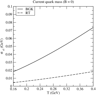
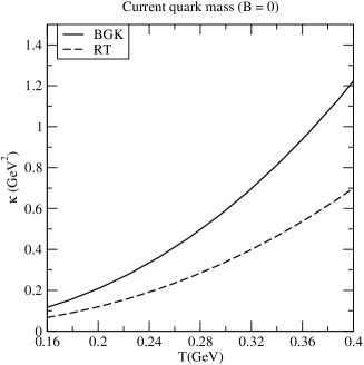
(a)	(b)

Figure 1: Variation of electrical ($\sigma_{el}$) (left) and thermal ($\kappa$) (right) conductivities with the temperature.

We have found that the modified BGK collision term enhances both charge and heat transport, compared to the collision term of relaxation type. To be specific, the ratio of $\sigma_{\rm el}$ in modified BGK collision term to the relaxation collision term is approximately 4.0, whereas the ratio for $\kappa$ is $\sim$ 1.76, implying that the collision integral is more sensitive to the charge transport.

2.3 Wiedemann-Franz law and Knudsen number in the absence of magnetic field

Wiedemann-Franz Law indicates that the transport of the charge and heat are not entirely different, rather the ratio of the transport coefficients in the respective cases is proportional to the temperature

$$\frac{\kappa}{\sigma_{el}}=L_{R}T,$$ (48)

and the proportional factor, $L_{R}$ is known as Lorentz number. The metals, which are good conductors of both electricity and heat, expectedly obey the Wiedemann-Franz law perfectly. There are some calculations in which the statement of the Wiedemann-Franz law have been violated, such as for the strongly-coupled QGP medium [36], two-flavor quark matter in the NJL model [35], and thermally populated electron-hole plasma in graphene, describing the signature of a Dirac fluid [37].

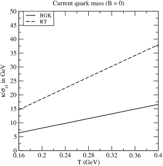
(a)	(b)

Figure 2: Variation of the ratio of the thermal conductivity to the electrical conductivity ($\kappa/\sigma_{el}$) and Lorenz number with temperature.

So far we have discussed the transport of both heat and electricity due to the participation of quarks only, thus it becomes reasonable to think that the heat and charge transport are not mutually exclusive as per the statement of Wiedemann-Franz law. In fact, they are found to obey the aforesaid law, as seen in Figure 2(a). Although the ratio, $\kappa/\sigma_{\rm el}$ is found to vary almost linearly with the temperature in Figure 2(a), but the actual behaviour of the interplay of heat and charge transport can be better understood through the Lorenz number, $L_{R}$ (=$\kappa/(\sigma_{\rm el}T)$). The Lorenz number initially increases monotonically in relatively smaller temperature and behaves constant in the high temperature, as seen in Figure 2(b). The effect of collision terms seen in the conductivities (in Figure 1) get also reflected into the relative behaviour through the ratio, $\kappa/\sigma_{\rm el}$ and in the Lorenz number, $L_{R}$ as well, where the relaxation collision integral is found to dominate over the modified BGK collision integral.

The validity of the assumption of a system to be in local equilibrium is tested with the help of the Knudsen number ($\Omega$). It is defined as the ratio of the mean free path $(\lambda)$ to the characteristic length scale $(L)$ of the system as

$$\Omega=\frac{\lambda}{L}.$$ (49)

The mean free path, $\lambda$ is computed from the thermal conductivity of the medium as

$$\lambda=\frac{3\kappa}{{\rm v_{rel}}C_{V}},$$ (50)

where $C_{V}$ is the specific heat of the medium and ${\rm v_{rel}}$ is the relative speed. The specific heat is contributed both by quarks and gluons,

$$C_{V}=C_{V}^{q}+C_{V}^{g},$$ (51)

where the quark contribution is

$$C_{V}^{q} = \frac{\partial\epsilon^{q}}{\partial T},$$ (52)

$$= \frac{\beta^{2}}{\pi^{2}}\sum g_{i}\int dp~{}p^{2}\omega_{i}^{2}f_{\rm eq,i}(1-f_{\rm eq,i}),$$

and the gluon contribution is

$$C_{V}^{g} = \frac{\partial\epsilon^{g}}{\partial T},$$ (53)

$$= \frac{\beta^{2}g_{g}}{2\pi^{2}}\int dp~{}p^{2}\omega_{g}^{2}f_{g}(1+f_{g}),$$

where $f_{g}$ is the gluon distribution function, given by

$$f_{g}=\frac{1}{e^{\beta\omega_{g}}-1}.$$ (54)

Finally, we have computed the Knudsen number as a function of temperature in Figure 3(a), wherein the modified BGK collision term is found to dominate over its counterpart (RT) and can be understood from the behaviour of $\kappa$. The magnitude of $\Omega$ is seen much lesser than one and decreases with the temperature, thus ensures the validity of the system being in local equilibrium. This can be understood by the competition between $C_{V}$, which is measure of the heat content, and $\kappa$, a measure of the ease by which the heat can be transported in the system. $\Omega$ becomes smaller than one because both the magnitude and the rate of increase of $C_{V}$ with $T$ is greater than the same in $\kappa$ (seen in Figure3(b)).

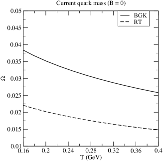
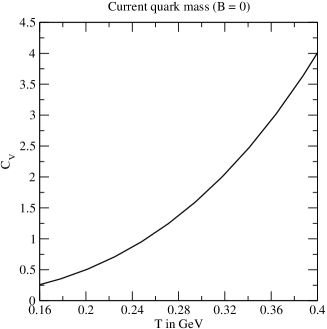
(a)	(b)

Figure 3: Variation of the Knudsen number $(\Omega)$ and specific heat with temperature.

Thus, the sections 2.1 and 2.2 decipher the effect of the modified BGK collision term on the transport coefficients of the charge and heat, which, in turn, do the same for the Lorenz and Kundsen number in section 2.3. In next section(s) 2.4 and 2.5, we will see how the strong magnetic field modulate the effect of collision term on the charge and heat transport, respectively. This, in turn, will explore the same on the Lorenz and Knudsen number in Section 2.6.

2.4 Electrical conductivity in a background of strong magnetic field

In the presence of the strong magnetic field ($B$), the motion of quarks becomes purely longitudinal (in the direction of magnetic field, say 3-direction), which is evident from the quantum mechanical relation: $\omega_{i}=\sqrt{p_{3}^{2}+m_{i}^{2}}$ in strong $B$. This is because that only the lowest Landau level ($n=0$) is populated due to the larger value of $|q_{i}B|$ ($\gg T^{2}$). Thus, when the medium is perturbed by the external magnetic field in 3-direction, an electromagnetic current is generated only in the longitudinal (3-) direction,

$$J_{3}=2\sum_{i}q_{i}g_{i}\frac{|q_{i}B|}{4\pi^{2}}\int{dp_{3}}~{}\frac{p_{3}}{\omega_{i}}~{}\delta f^{B}_{i}(x,p).$$ (55)

Thus, the electrical conductivity relates the longitudinal current generated to the electrical field as

$$J_{3}=\sigma_{el}~{}E_{3},$$ (56)

where $\sigma_{\rm el}$ is the longitudinal component of the electrical conductivity of the medium and the term ‘longitudinal’ refers with respect to the direction of the strong magnetic field. The component of $\sigma_{\rm el}$ transverse to the magnetic field vanishes due to Landau quantization of the transverse motion in the strong magnetic field[48].

Therefore, in order to obtain $\sigma_{\rm el}$, we need to know the infinitesimal deviation of the medium ($\delta f^{B}_{i}$) in the presence of strong magnetic field. As earlier, this will be obtained by solving the Boltzmann equation (4) with the linearized collision integral. So, we start with the Boltzmann equation in a strong magnetic field as

$$p^{0}\frac{\partial f^{B}_{i}}{\partial x^{0}}+p^{3}\frac{\partial f^{B}_{i}}{\partial x^{3}}+q_{i}F^{03}p_{3}\frac{\partial f^{B}_{i}}{\partial p^{0}}+q_{i}F^{30}p_{0}\frac{\partial f^{B}_{i}}{\partial p^{3}}=-p^{\mu}u_{\mu}\nu_{i}^{B}\left(f_{i}^{B}-n_{i}^{B}{n_{\mathrm{e}q,i}^{B~{}-1}}f_{\mathrm{e}q,i}^{B}\right),$$ (57)

where $n_{i}^{B}$ is the perturbed density and $n_{\mathrm{e}q,i}^{B}$ is the equilibrium density in the presence of the strong magnetic field, which is given by

$$n_{\mathrm{e}q,i}^{B} = \frac{g_{i}|q_{i}B|}{4\pi^{2}}\int dp_{3}~{}f_{\rm eq,i}^{B},$$ (58)

with the equilibrium distribution function

$$f_{\mathrm{e}q,i}^{B}=\frac{1}{e^{\beta\omega_{i}}+1}.$$ (59)

The collision frequency in a strong $B$, $\nu_{i}^{B}$ runs with the (longitudinal) momentum ($p_{3}$), unlike that $\tau_{i}$ in pure thermal medium ((9)) is independent of momentum. Moreover, $\tau_{i}^{B}$ depends strongly on the magnetic field and weakly on the temperature because the dominant scale assigned to quark degrees of freedom in a thermal medium in strong $B$, being the magnetic field, in the same way that the temperature dominates in a thermal medium in the absence of magnetic field. The collision time, the inverse of the collisional frequency ($\nu_{i}^{B}$), in strong $B$ has been calculated recently in [49]

$$\tau_{i}^{B}(p_{3};T,|q_{i}B|)=\frac{\omega_{i}(e^{\beta\omega_{i}}-1)}{\alpha_{s}C_{F}m_{i}^{2}(e^{\beta\omega_{i}}+1)}{\left(\int\frac{dp^{\prime}_{3}}{\omega^{\prime}_{i}(e^{\beta\omega^{\prime}_{i}}+1)}\right)}^{-1},$$ (60)

where $C_{F}$ (=4/3) is the Casimir factor and the strong coupling, $\alpha_{s}$ now runs with the magnetic field only

$$\alpha_{s}(|q_{f}B|)=\frac{1}{(\alpha^{0}(\mu_{0}))^{-1}+\frac{11N_{C}}{12\pi}\ln\left(\frac{{\rm k_{z}}^{2}+M_{B}^{2}}{\mu_{0}^{2}}\right)+\frac{1}{3\pi}\sum_{i}\frac{|q_{i}B|}{\sigma}},$$ (61)

where

$$\alpha^{0}(\mu_{0})=\frac{12\pi}{11N_{C}\ln\left(\frac{\mu_{0}^{2}+M_{B}^{2}}{\Lambda_{V}^{2}}\right)}.$$

Here $M_{B}$ is infrared mass (1 GeV) and $\Lambda_{V}$ and $\mu_{0}$ are taken as 0.385 GeV and 1.1 GeV, respectively and ${\rm k_{z}}=0.1\sqrt{eB}$.

Thus, going to the next approximation beyond the initial (equilibrium) configuration, the total time-derivative of the probability distribution in Boltzmann equation in the presence of strong magnetic field is simplified into

$$\frac{df^{B}_{i}}{dt}=-2q_{i}\beta p_{3}E_{3}f_{\mathrm{e}q,i}^{B}\left(1-f_{\mathrm{e}q,i}^{B}\right),$$ (62)

wherein the partial derivatives of the equilibrium distribution, $f_{\mathrm{e}q,i}^{B}$ have been used:

$$\frac{\partial f_{\mathrm{e}q,i}^{B}}{\partial p^{0}} = -\frac{1}{T}f_{\mathrm{e}q,i}^{B}(1-f_{\mathrm{e}q,i}^{B}),$$ (63)

$$\frac{\partial f_{\mathrm{e}q,i}^{B}}{\partial p^{3}} = -\frac{p_{3}}{Tp_{0}}f_{\rm eq,i}^{B}(1-f_{\rm eq,i}^{B}).$$ (64)

Next, linearizing the collision integral, the Boltzmann equation gives the transcendental equation for the linear infinitesimal disturbance, $\delta f_{i}^{B}$ for $i$-th flavour as

$$\delta f_{i}^{B}-g_{i}{n_{\mathrm{e}q,i}^{B}}^{-1}f_{\rm eq,i}^{B}\int_{p_{3}}\delta f_{i}^{B}=2q_{i}\beta\tau_{i}^{B}\frac{p_{3}E_{3}}{\omega_{i}}f_{\rm eq,i}^{B}\left(1-f_{\rm eq,i}^{B}\right),$$ (65)

which yields the disturbance, $\delta f_{i}^{B}$ up to the first-order (neglecting ${\cal O}{(\delta f_{i}^{B})}^{2}$ terms) as

$$\delta f_{i}^{B}=\delta f_{i}^{B(0)}+g_{i}{n_{\mathrm{e}q,i}^{B}}^{-1}f_{\rm eq,i}^{B}\int_{p^{\prime}_{3}}\delta f_{i}^{B(0)},$$ (66)

where

$$\delta f_{i}^{B(0)}=\frac{2q_{i}\beta\tau_{i}^{B}}{\omega_{i}}p_{3}E_{3}~{}f_{\rm eq,i}^{B}(1-f_{\rm eq,i}^{B}).$$ (67)

Therefore, we can now calculate the current density, $J_{3}$ from (55) with $\delta f_{i}^{B}$ taken from (66) as

$$J_{3} = \frac{\beta}{\pi^{2}}\sum_{i}q_{i}^{2}g_{i}|q_{i}B|\left[\int{dp_{3}}\frac{p_{3}^{2}}{\omega_{i}^{2}}~{}\tau_{i}^{B}(p_{3})~{}f_{\rm eq,i}^{B}(1-f_{\rm eq,i}^{B})\right.$$ (68)

$$\left.+g_{i}{n_{\mathrm{e}q,i}^{B}}^{-1}\int{dp_{3}}\frac{p_{3}}{\omega_{i}}f_{\rm eq,i}^{B}\int_{p^{\prime}_{3}}\frac{p^{\prime}_{3}}{\omega_{i}}~{}\tau_{i}^{B}(p_{3}^{\prime})~{}f_{\rm eq,i}^{B}~{}(1-f_{\rm eq,i}^{B})\right]E_{3}.$$

So we extract the coefficient of the electric field, $E_{3}$ as the electrical conductivity of a thermal QCD medium in a strong $B$, which, in modified BGK collision term, yields as the sum of the contribution due to the RT collision term and a correction term

$$\sigma_{\rm el}^{B}=\sigma_{\rm el}^{B,\rm RT}+\sigma^{B,\rm Corr}_{el},$$ (69)

where

$$\sigma^{B,\rm RT}_{el} = \frac{\beta}{\pi^{2}}\sum_{i}q_{i}^{2}g_{i}|q_{i}B|\int{dp_{3}}\frac{p_{3}^{2}~{}\tau_{i}^{B}}{\omega_{i}^{2}}f_{\mathrm{e}q,i}^{B}(1-f_{\mathrm{e}q,i}^{B}),$$ (70)

$$\sigma^{B,\rm Corr}_{el} = \frac{\beta}{\pi^{2}}\sum_{i}q_{i}^{2}g^{2}_{i}|q_{i}B|{n_{\mathrm{e}q,i}^{B}}^{-1}\left[\int{dp_{3}}\frac{p_{3}}{\omega_{i}}f_{\rm eq,i}^{B}\int_{p^{\prime}_{3}}\frac{p^{\prime}_{3}}{\omega_{i}}~{}\tau_{i}^{B}(p_{3}^{\prime})~{}f_{\rm eq,i}^{B}~{}(1-f_{\rm eq,i}^{B})\right],$$ (71)

where the correction, $\sigma^{\rm B,Corr}_{\rm el}$ is found to be positive, implying that even in the presence of strong magnetic field, the dominance of modified BGK collision integral over RT Collision integral is still retained in the charge transport.

2.5 Thermal conductivity in a strong magnetic field

In this section, we will calculate the thermal conductivity of a hot QCD medium in the presence of strong magnetic field. Thus, we closely follow the previous section 2.2. In the presence of the strong magnetic field ($B$), only the component along the direction of the magnetic field (3-direction) survives and takes the form

$$Q_{3}=\sum_{i}\frac{g_{i}|q_{i}B|}{2\pi^{2}}\int{dp_{3}}~{}\frac{p_{3}}{\omega_{i}}~{}(\omega_{i}-h_{i}^{B})~{}\delta f_{i}^{B},$$ (72)

where

$$h_{i}^{B} = \frac{(\epsilon_{i}^{B}+P_{i}^{B})}{n_{eq,i}^{B}},$$ (73)

$$\epsilon_{i}^{B} = \frac{g_{i}|q_{i}B|}{4\pi^{2}}\int dp_{3}~{}\omega_{i}f_{\rm eq,i}^{B},$$ (74)

$$P_{i}^{B} = \frac{g_{i}|q_{i}B|}{12\pi^{2}}\int dp_{3}\frac{p_{3}^{2}}{\omega_{i}}~{}f_{\rm eq,i}^{B}.$$ (75)

On the other hand, the spatial component of heat flow vector (43) in the Navier-Stokes equation, takes the form in a strong $B$ (along the 3-direction),

$$Q^{i}_{3} = -\kappa\left[\frac{\partial T}{\partial x_{3}}-\frac{T}{n^{B}_{eq,i}h^{B}_{i}}\frac{\partial P_{i}}{\partial x_{3}}\right],$$ (76)

$$= \kappa\left[{\partial_{3}T}-\frac{T}{n^{B}_{\mathrm{e}q,i}h^{B}_{i}}{\partial_{3}P_{i}}\right],$$

where the coefficient, $\kappa$ is the thermal conductivity. Therefore, once we compute the heat flow vector from the kinetic theory (72) and express it in the form (76), we could then pick up the coefficient of gradient term as $\kappa$. So we start with the Boltzman equation in the presence of strong magnetic field, in terms of velocity and temperature gradients through the chain rule of differentiation,

$$p^{\mu}\frac{\partial f^{B}_{i}}{\partial T}\frac{\partial T}{\partial x^{\mu}}+p^{\mu}\frac{\partial f^{B}_{i}}{\partial p^{0}}\frac{\partial(p^{\nu}u_{\nu})}{\partial x^{\mu}}+q_{i}\left[F^{03}p_{3}\frac{\partial f^{B}_{i}}{\partial p^{0}}+F^{30}p_{0}\frac{\partial f^{B}_{i}}{\partial p^{3}}\right]=C[f].$$ (77)

For vanishingly small value of $\mu_{i}$, the infinitesimal deviation, $\delta f_{i}^{B}$ is obtained by solving the Boltzman equation, after linearizing the collision integral with respect to the deviation (see the Appendix B)

$$\delta f_{i}^{B}=\delta f_{i}^{B(1)}+g_{i}{n_{\mathrm{e}q,i}^{B}}^{-1}f_{\rm eq,i}^{B}\int_{p^{\prime}_{3}}\delta f_{i}^{B(1)},$$ (78)

where

$$\delta f_{i}^{B(1)} = -\frac{f_{\rm eq,i}^{B}(1-f_{\rm eq,i}^{B})\tau_{i}^{B}}{T}\left[\frac{p^{0}}{T}\partial_{0}T+\frac{(p^{0}-h_{i}^{B})}{p^{0}}\frac{p^{3}}{T}\left(\partial_{3}T-\frac{T}{n^{B}_{\mathrm{e}q,i}h_{i}^{B}}\partial_{3}P_{i}\right)+T\partial_{0}\left(\frac{\mu_{i}}{T}\right)\right.$$ (79)

$$\left.-\frac{p^{3}p^{\nu}}{p^{0}}\partial_{3}u_{\nu}-2q_{i}\frac{E_{3}p_{3}}{p^{0}}\right].$$

Now we are in a position to calculate the heat-flow vector ($Q_{3}$) in the presence of strong magnetic field from the kinetic theory by plugging $\delta f_{i}^{B}$ in (72),

$$Q_{3} = \sum_{i}\frac{g_{i}|q_{i}B|}{2\pi^{2}}\int{dp_{3}}~{}\frac{p_{3}}{\omega_{i}}~{}(\omega_{i}-h_{i}^{B})\left[\left\{\frac{f_{\rm eq,i}^{B}(1-f_{\rm eq,i}^{B})\tau_{i}^{B}}{T}\frac{(p^{0}-h_{i}^{B})}{p^{0}}\frac{p_{3}}{T}\right.\right.$$ (80)

$$\left.\left.+g_{i}{n_{\mathrm{e}q,i}^{B}}^{-1}f_{\rm eq,i}^{B}\int_{p^{\prime}_{3}}\frac{f_{\rm eq,i}^{B}(1-f_{\rm eq,i}^{B})\tau_{i}^{B}}{T}\frac{(p^{0}-h_{i}^{B})}{p^{0}}\frac{p_{3}}{T}\right\}\left(\partial_{3}T-\frac{T}{n^{B}_{\mathrm{e}q,i}h_{i}^{B}}\partial_{3}P_{i}\right)\right.$$

$$\left.+\left(\frac{f_{\rm eq,i}^{B}(1-f_{\rm eq,i}^{B})\tau_{i}^{B}}{T}+g_{i}{n_{\mathrm{e}q,i}^{B}}^{-1}f_{\rm eq,i}^{B}\int_{p^{\prime}_{3}}\frac{f_{\rm eq,i}^{B}(1-f_{\rm eq,i}^{B})\tau_{i}^{B}}{T}\right)\left\{\frac{p^{0}}{T}\partial_{0}T+T\partial_{0}\left(\frac{\mu}{T}\right)\right.\right.$$

$$\left.\left.-\frac{p^{3}p^{\nu}}{p^{0}}\partial_{3}u_{\nu}-2q_{i}\frac{E_{3}p_{3}}{p^{0}}\right\}\right].$$

Thus, we obtain $\kappa$ from the heat flow vector, by matching the coefficient of the gradient of thermal potential in the Navier-Stokes equation (76) with the same in the kinetic theory (80) and similar to the absence of (strong) magnetic field, $\kappa$ in modified collision term is decomposed into the contribution due to collision term of relaxation type and a correction term

$$\mathbf{\kappa}^{B}=\kappa^{\rm B,RT}+\kappa^{\rm B,Corr},$$ (81)

where

$$\kappa^{\rm B,RT} = \frac{\beta^{2}}{2\pi^{2}}\sum_{i}{g_{i}|q_{i}B|}\int{dp_{3}}\frac{p_{3}^{2}~{}\tau_{i}^{B}}{\omega_{i}^{2}}(\omega_{i}-h_{i}^{B})^{2}f_{\rm eq,i}^{B}(1-f_{\rm eq,i}^{B}),$$ (82)

$$\kappa^{\rm B,Corr} = \frac{\beta^{2}}{2\pi^{2}}\sum_{i}{g^{2}_{i}|q_{i}B|}{n_{\mathrm{e}q,i}^{B}}^{-1}\left[\int{dp_{3}}\frac{p_{3}}{\omega_{i}}(\omega_{i}-h_{i}^{B})f_{\rm eq,i}^{B}\int_{p^{\prime}_{3}}\frac{p^{\prime}_{3}~{}\tau_{i}^{B}(p^{\prime}_{3})}{\omega^{\prime}_{i}}(\omega^{\prime}_{i}-h_{i}^{B})f_{\rm eq,i}^{B}(1-f_{\rm eq,i}^{B})\right],$$ (83)

where the correction factor in strong $B$, unlike in the absence of magnetic field (47), becomes negative. As a result, the dominance of the modified BGK collision term over the RT collision term is lost.

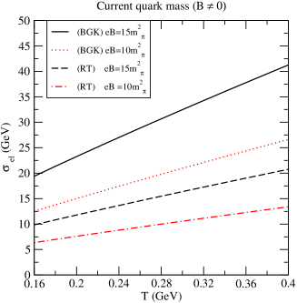
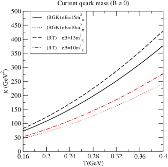
(a)	(b)

Figure 4: Variation of electrical ($\sigma_{el}$) (left) and thermal ($\kappa$) (right) conductivities with the temperature.

To see how the strong magnetic field modulates the effect of collision term on the electrical and thermal conductivities pictorially, we have computed them as a function of temperature at increasing strengths of magnetic fields: $eB=10m_{\pi}^{2}$ and $eB=15m_{\pi}^{2}$. The observations are two folds: i) The strong $B$ enhances overall magnitudes of both $\sigma_{\rm el}$ and $\kappa$ by orders of two-to-three in high and low temperature region, respectively. Especially, the $B$ affects the charge transport with RT collision terms. ii) it flips the dominance of the collision terms from BGK to RT in heat transport. This is due to the fact that unlike in $B=0$ case, the correction term in (83) becomes negative, because the dispersion relation in strong $B$ makes the relaxation-time momentum dependent, which in low momentum limit ($p_{3}\rightarrow 0$) becomes constant and in high momentum limit ($p_{3}\rightarrow\infty$), increases indefinitely with $p_{3}$. As a result, the second integral in the correction, $\kappa^{\rm B,Corr}$ becomes positive and makes the overall correction negative (because the first integral - $\int_{p_{3}}\frac{p_{3}}{\omega_{i}}(\omega_{i}-h_{i}^{B})f^{B}_{\mathrm{e}q,i}$ is always negative).

Thus, having deciphered the sole effects of collision term and strong magnetic field on the electrical and thermal conductivities for a medium consisting of noninteracting/ideal partons, we will examine how the abovementioned affects modulates the interplay between heat and charge transport and the affiliated transport coefficient derived by them. Thus, the relative behaviour is checked by the ratio, $\kappa/\sigma_{\rm el}$ (and the Lorenz number, $L_{R}$) and the derived coefficient is the equilibration factor, quantified by the Knudsen number ($\Omega$). It is found that both the ratio, $\kappa/\sigma_{\rm el}$ and the Knudsen number are dominated by the RT collision term over the BGK term in a fixed (strong) $B$ whereas for a collision term, the effect of strong $B$ can be understood as follows:

One of the factor in the denominator of the Knudsen number is the specific heat and the quark contribution to the specific heat gets severely affected due to the dimensional reduction in strong $B$ as

$$C_{V}^{q} = \frac{\partial\varepsilon^{q}}{\partial T}$$ (84)

$$= \frac{\partial(u_{\alpha}T^{\alpha\beta}u_{\beta})}{\partial T}$$

$$= \beta^{2}\sum_{i}\frac{g_{i}|q_{i}B|}{2\pi^{2}}\int dp_{3}~{}\omega_{i}^{2}f_{\rm eq,i}^{B}(1-f_{\rm eq,i}^{B}),$$ (85)

resulting an overall decrease in the specific heat. As a consequence, the Knudsen number becomes too large to understand physically because the validation of the equilibrium thermodynamics requires $\Omega$ to be less than one because the large Knudsen number contradicts with the basic idea of near-equilibrium assumption that is used to linearize the kinetic equation. This motivates us to treat the partons interacting because the interactions among the partons in a thermal medium generate the masses, which, in turn, behaves as an infrared cut-off in the crosssection of $gg\rightarrow gg$ scattering, responsible for bringing the system into equilibrium. Hence, the unusually larger value of relaxation-time in a strong magnetic field becomes finite and causes the thermal conductivity smaller. This possible way-out resonates with the idea that the more the constituents interact amongst themselves the quicker the system achieves the equilibrium. Thus, the necessity of quasiparticle description of partons gets motivated in the next section.

3 Charge and heat transport with the quasiparticle description of partons

The transport of charge and heat in a thermal QCD medium with the noninteracting quarks and gluons in strong $B$ hereinabove described yields unusually large values of electrical and thermal conductivities and the affiliated coefficients (Lorenz number, Knudsen number) therein, which defy physical interpretation. As we know, the thermal medium generically ascribes the masses to the constituents, which motivates us for a quasiparticle description of partons participating in the transport phenomena in this section.

3.1 Quasiparticle description of partons

The idea of quasiparticle description (QPD) of a parton in a medium is to encrypt the interaction of the given parton with the remaining partons in terms of its in-medium mass, known as quasiparticle masses or thermal masses and then treat these quasiparticles as noninteracting particles. In a sense, at the scale of the quasiparticle mass, the independent (single)behaviour of partons ceases to exist and the collective behaviour of the medium sets in. There are some variants of quasiparticle description where the interactions amongst themselves are also taken into account. Different versions of quasi-particle description exist in the literature based on different effective theories, such as thermodynamically consistent quasi particle model [50], Nambu-Jona-Lasinio (NJL) model and its extension Polyakov NJL (PNJL model [51, 52, 53], Gribov-Zwanziger quantization model [54, 55]. In this work we employ the medium generated masses for quarks and gluons in the framework of perturbative QCD at finite temperature and/or strong $B$ from the poles of resummed propagators calculated from the respective self-energies.

Let us start with a thermal QCD medium in the absence of magnetic field. The quasiparticle masses of $i$-th flavour is written phenomenologically as [50]

$$m_{i}^{2}=m_{i0}^{2}+\sqrt{2}m_{i0}m_{iT}+m_{iT}^{2},$$ (86)

where $m_{i,0}$ and $m_{i,T}$ are the current quark mass and thermally generated mass respectively. The thermal mass for the quarks have been calculated in hard-thermal-loop perturbation theory with the temperature as the hardest scale [56, 57] as

$$m_{iT}^{2}=\frac{g^{\prime 2}T^{2}}{6},$$ (87)

where $g^{\prime}$ is the strong coupling which runs with the temperature (eqn. (10)). Similarly the gluons also acquire a thermal mass, which is also calculated as

$$m_{g}^{2}=\frac{g^{\prime 2}T^{2}}{6}\left(N_{C}+\frac{N_{f}}{2}\right).$$ (88)

Now, for thermal QCD medium in the presence of strong magnetic field, the form of thermal/quasiparticle mass can be generalized as

$$m_{i}^{2}=m_{i0}^{2}+\sqrt{2}m_{i0}m_{iT,B}+m_{iT,B}^{2},$$ (89)

where the thermal mass, $m_{iT,B}$ are obtained from the dispersion relation of the full quark propagator in strong $B$, by solving the Dyson-Schwinger equation self-consistently:

$$S^{-1}(p_{\parallel})=\gamma^{\mu}p_{\parallel\mu}-\Sigma(p_{\parallel}).$$ (90)

The $\Sigma(p_{\parallel})$ in the above is the quark self-energy, which needs to be evaluated at finite temperature in the presence of strong $B$. Up to one-loop, its expression is given by

$$\Sigma(p)=-\frac{4}{3}g^{2}i\int{\frac{d^{4}k}{(2\pi)^{4}}}\left[\gamma_{\mu}{S(k)}\gamma_{\nu}{D^{\mu\nu}(p-k)}\right],$$ (91)

where the QCD coupling, $g$ now runs with the magnetic field, mentioned in(61)).

The quark propagator, $S(k)$ in an external magnetic field is calculated [58] by the Schwinger proper-time method in the momentum space in terms of Laguerre polynomials,

$$iS_{n}(k)=\sum_{n}\frac{-id_{n}(\alpha)D+d^{\prime}_{n}(\alpha)\bar{D}}{k_{\|}^{2}-m^{2}_{f}+2n|q_{f}B|}+i\frac{\gamma\cdot k_{\bot}}{k_{\bot}^{2}}~{},$$ (92)

where the label, $n(=0,1,2,\cdots)$ denotes the Landau levels. The above symbols are defined as [59]

$$D=(m_{f}+\gamma\cdot k_{\|})+\gamma\cdot k_{\bot}\frac{m_{f}^{2}-k_{\|}^{2}}{k_{\|}^{2}},$$

$$\bar{D}=\gamma_{1}\gamma_{2}(m_{f}+\gamma\cdot k_{\|}),$$

$$d_{n}(\alpha)=(-1)^{n}e^{-\alpha}C_{n}(2\alpha),$$

$$d^{{}^{\prime}}_{n}(\alpha)=\frac{\partial d_{n}}{\partial\alpha},$$

with the dimensionless variable, $\alpha$ = $k_{\bot}^{2}/|q_{f}B|$. The $C_{n}$’s are expressed in terms of Laguerre polynomial ($L_{n}$)

$$C_{n}(2\alpha) = L_{n}(2\alpha)-L_{n-1}(2\alpha).$$

In the strong magnetic limit, only the lowest Landau levels get populated, so $S(k)$ is simplified into a form

$$S(k)=ie^{-\frac{k^{2}_{\perp}}{|q_{i}B|}}\frac{\left(\gamma^{0}k_{0}-\gamma^{3}k_{z}+m_{i}\right)}{k^{2}_{\parallel}-m^{2}_{i}}\left(1-\gamma^{0}\gamma^{3}\gamma^{5}\right),$$ (93)

where the four vectors are defined with the metric tensors: $g^{\mu\nu}_{\perp}={\rm{diag}}(0,-1,-1,0)$ and $g^{\mu\nu}_{\parallel}={\rm{diag}}(1,0,0,-1)$,

$$k_{\perp\mu}\equiv(0,k_{x},k_{y},0),~{}~{}k_{\parallel\mu}\equiv(k_{0},0,0,k_{z})~{}.$$

The gluon propagator, $D^{\mu\nu}(p-k)$ is not affected by the magnetic field, so its takes the form

$$D^{\mu\nu}(p-k)=\frac{ig^{\mu\nu}}{(p-k)^{2}}~{}.$$ (94)

In imaginary-time formalism, the quark self-energy (91) in strong magnetic field can be simplified into (see the Appendix C)[34]

$$\Sigma(p_{\parallel})=\frac{g^{2}|q_{i}B|}{3\pi^{2}}\left[\frac{\pi T}{2m_{i}}-\ln(2)\right]\left[\frac{\gamma^{0}p_{0}}{p_{\parallel}^{2}}+\frac{\gamma^{3}p_{z}}{p_{\parallel}^{2}}+\frac{\gamma^{0}\gamma^{5}p_{z}}{p_{\parallel}^{2}}+\frac{\gamma^{3}\gamma^{5}p_{0}}{p_{\parallel}^{2}}\right],$$ (95)

which can further be decomposed in the covariant form as [60, 22]

$$\Sigma(p_{\parallel})=A\gamma^{\mu}u_{\mu}+B\gamma^{\mu}b_{\mu}+C\gamma^{5}\gamma^{\mu}u_{\mu}+D\gamma^{5}\gamma^{\mu}b_{\mu},$$ (96)

where $A,B,C$ and D are the form factors. $u^{\mu}(1,0,0,0)$ and $b^{\mu}(0,0,0,-1)$ represents the direction of the heat bath and magnetic field respectively. These vectors are behind the breaking of the Lorentz and the rotational symmetry respectively. The form factors can be calculated in LLL approximation as

$$A = \frac{1}{4}{\rm Tr}[\Sigma\gamma^{\mu}u_{\mu}]=\frac{g^{2}|q_{i}B|}{3\pi^{2}}\left[\frac{\pi T}{2m_{i}}-\ln{(2)}\right]\frac{p_{0}}{p_{\parallel}^{2}},$$ (97)

$$B = -\frac{1}{4}{\rm Tr}[\Sigma\gamma^{\mu}b_{\mu}]=\frac{g^{2}|q_{i}B|}{3\pi^{2}}\left[\frac{\pi T}{2m_{i}}-\ln{(2)}\right]\frac{p_{z}}{p_{\parallel}^{2}},$$ (98)

$$C = \frac{1}{4}{\rm Tr}[\gamma^{5}\Sigma\gamma^{\mu}u_{\mu}]=-\frac{g^{2}|q_{i}B|}{3\pi^{2}}\left[\frac{\pi T}{2m_{i}}-\ln{(2)}\right]\frac{p_{z}}{p_{\parallel}^{2}},$$ (99)

$$D = -\frac{1}{4}{\rm Tr}[\gamma^{5}\Sigma\gamma^{\mu}b_{\mu}]=-\frac{g^{2}|q_{i}B|}{3\pi^{2}}\left[\frac{\pi T}{2m_{i}}-\ln{(2)}\right]\frac{p_{0}}{p_{\parallel}^{2}},$$ (100)

we get $C=-B$ and $D=-A$. In terms of chiral projection operators, the quark self energy takes the form

$$\Sigma(p_{\parallel})=P_{R}[(A+C)\gamma^{\mu}u_{\mu}+(B+D)\gamma^{\mu}b_{\mu}]P_{L}+P_{L}[(A-C)\gamma^{\mu}u_{\mu}+(B-D)\gamma^{\mu}b_{\mu}]P_{R},$$ (101)

$$\Sigma(p_{\parallel})=P_{R}[(A-B)\gamma^{\mu}u_{\mu}+(B-A)\gamma^{\mu}b_{\mu}]P_{L}+P_{L}[(A+B)\gamma^{\mu}u_{\mu}+(B+A)\gamma^{\mu}b_{\mu}]P_{R},$$ (102)

where $P_{R}=(1+\gamma^{5})/2$ and $P_{L}=(1-\gamma^{5})/2$ are the right handed and left handed chiral projection operators respectively. The effective quark propagator in terms of the chiral projection operators can be written as

$$S^{-1}(p_{\parallel})=P_{R}\gamma^{\mu}X_{\mu}P_{L}+P_{L}\gamma^{\mu}Y_{\mu}P_{R},$$ (103)

where

$$\gamma^{\mu}X_{\mu} = \gamma^{\mu}p_{\parallel\mu}-(A-B)\gamma^{\mu}u_{\mu}-(B-A)\gamma^{\mu}b_{\mu},$$ (104)

$$\gamma^{\mu}Y_{\mu} = \gamma^{\mu}p_{\parallel\mu}-(A+B)\gamma^{\mu}u_{\mu}-(B+A)\gamma^{\mu}b_{\mu}.$$ (105)

The effective propagator can be further written as

$$S(p_{\parallel})=\frac{1}{2}\left[P_{R}\frac{\gamma^{\mu}Y_{\mu}}{Y^{2}/2}P_{L}+P_{L}\frac{\gamma^{\mu}X_{\mu}}{X^{2}/2}P_{R}\right]$$ (106)

where

$$\frac{X^{2}}{2}=X_{1}^{2}=\frac{1}{2}\left[p_{0}-(A-B)\right]^{2}-\frac{1}{2}\left[p_{z}+(B-A)\right]^{2}~{},$$ (107)

$$\frac{Y^{2}}{2}=Y_{1}^{2}=\frac{1}{2}\left[p_{0}-(A+B)\right]^{2}-\frac{1}{2}\left[p_{z}+(B+A)\right]^{2}~{}.$$ (108)

We take static limit ($p_{0}=0,~{}p_{z}\rightarrow 0$) of either $X_{1}^{2}$ or $Y_{1}^{2}$ (which are equal in this limit) to get thermal mass (squared) at finite temperature and strong magnetic field as

$$m_{iT,B}^{2}=\frac{g^{2}|q_{i}B|}{3\pi^{2}}\left[\frac{\pi T}{2m_{i}}-\ln{(2)}\right],$$ (109)

which depends on both the magnetic field and the temperature.

3.2 Electrical and Thermal Conductivity in B=0: Wiedemann Franz Law and Knudsen Number

In kinetic theory approach of evaluating the transport coefficients, the quasiparticle description (QPD) of partons encodes the interactions present in the medium through the dispersion relation, where the vacuum masses in noninteracting scenario get modified by the quasiparticle masses (which depend on the $T$ and $B$). Thus, the occupation probability (distribution function) gets modified through the dispersion relation, which, in turn, will affect the transport process of heat, charge etc. In short, we follow the derivation of the conductivities and their derived coefficients in QPD scenario, in the same way as was done in the previous section, except that the distribution function now involves the masses generated by the medium. We have found that the forms of the conductivities as in noninteracting scenario remain the same, so we compute the electrical and thermal conductivities as a function of temperature with the in-medium masses (87) and (88) for quarks and gluons in the respective distribution functions (8) and (54), respectively. It is found that both charge and heat

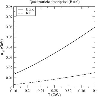
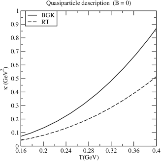
(a)	(b)

Figure 5: Variation of electrical conductivity $\sigma_{el}$ (left) and thermal conductivity $\kappa$ (right) with respect to the temperature

transport get impeded due to the in-medium (heavier) masses of quarks (which reduce the mobility of the carriers), compared to the noninteracting scenario with current quark masses, which are reflected in the slight reduction of $\sigma_{\rm el}$ and $\kappa$ in Figure 5. However, the BGK collision term still retains the dominance over the RT collision term for both thermal and electrical conductivities, even in the QPD of partons.

Now we will see how the QPD of partons affect the ratio, $\kappa/\sigma_{\rm el}$ (and the Lorenz number as well) and the Knudsen number in the absence of magnetic field. The aforesaid discussion on the charge and heat transport helps to understand the slight decrease in the ratio ($\kappa/\sigma_{\rm el}$) and the Lorenz number in Figure 6 with respect to the noninteracting scenario (in Figure 2).

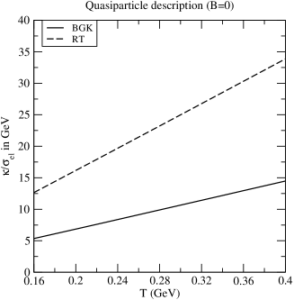
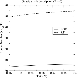
(a)	(b)

Figure 6: Variation of the ratio of the thermal conductivity to the electrical conductivity ($\kappa/\sigma_{el}$) and Lorenz number with temperature.

Similarly, the QPD of partons in the absence of magnetic field also reduces the Knudsen number a little bit, in comparison to noninteracting case (as in Figure 3(a)), which is mainly due to the opposite behaviour in thermal conductivity and specific heat in quasiparticle description (as seen in Figures 5(b) and 7(b), respectively). The reduction in $\Omega$ is in line with the fact that the more the interactions among the constituents the quicker the system comes to local equilibrium.

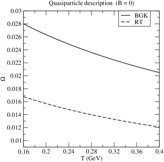
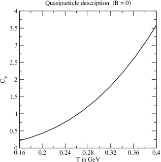
(a)	(b)

Figure 7: Variation of the Knudsen number ($\Omega$) and specific heat with temperature.

3.3 Electrical and Thermal Conductivity in $B\neq 0$: Wiedemann Franz Law and Knudsen Number

To see how the unusually larger values of $\sigma_{\rm el}$ and $\kappa$ for noninteracting partons in a strong $B$ (in Figure 4) could be affected by the QPD of partons, we have now computed them in Figure 8 with the in-medium quark masses at finite temperature and strong $B$ from (109).

We find that both $\sigma_{\rm el}$ and $\kappa$ gets reduced by an order three, compared to the noninteracting picture (Figure 4). The primary reason behind this observation lies in the dispersion relation of partons in strong $B$, where the collective oscillation sets in much bigger scale than in the absence of $B$. As a secondary reason, the dispersion relation, in turn, tames the relaxation-time, $\tau^{B}$ in strong $B$ (seen in Figure 11, which can be understood by the fact that the infra-red singularity in gluon-gluon cross-section in $\tau^{B}$ is cured by the the mass generated in the medium, which, in the presence of strong $B$, becomes much larger than in $B=0$ (seen in the Figure 12).

Table 1: Masses generated for $u$, $d$ and $s$ flavours in a thermal QCD medium in the absence and presence of strong $B$ background.

	$m_{i}$ (B=0)			$m_{i}$ (B $\neq 0$)
	u quark	d quark	s quark	u quark	d quark	s quark
	(GeV)	(GeV)	(GeV)	(GeV)	(GeV)	(GeV)
Low T	0.1464	0.1485	0.2275	0.7622	0.4187	0.1652
(0.16 GeV)
High T	0.2935	0.2992	0.3735	1.2156	0.6669	0.2224
(0.40 GeV)

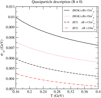
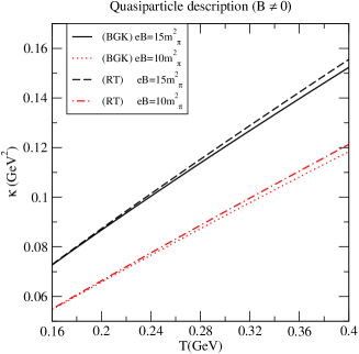
(a)	(b)

Figure 8: Variation of electrical ($\sigma_{el}$) (left) and thermal ($\kappa$) (right) conductivities with the temperature.

Finally, the aforesaid behaviour of $\sigma_{\rm el}$ and $\kappa$ in strong $B$ facilitates to understand the effect of QPD on the ratio, $\kappa/\sigma_{\rm el}$ and subsequently on the Lorenz number, $L_{R}$ in Figure 9(a) and Figure 9(b), respectively, wherein both of them get amplified. Last but not the least, the best reward of quasiparticle description gets reflected in the drastic reduction of Knudsen number, $\Omega$, which looks now feasible (as seen in Figure 10(a)). Earlier in noninteracting description, $\Omega$ in strong $B$ becomes much larger than one, implying that the system runs away from equilibrium. To understand the abovementioned behaviour of $\Omega$, we also compute the another factor in $\Omega$, the specific heat as a function of $T$ in the same description in Figure 10(b). Finally, the excerpts of our exploration is that the QPD of partons almost smears the effect of the collision terms, at least, on the heat transport ($\kappa$) in strong $B$, (as seen in 8 (b)), which is being translated into a interesting collision term dependence in the Lorenz number and Knudsen number in Figure 9 (b) and Figure 10 (a), respectively.

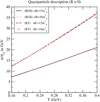
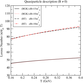
(a)	(b)

Figure 9: Variation of the ratio of the thermal conductivity to the electrical conductivity ($\kappa/\sigma_{el}$) and Lorentz number with temperature.

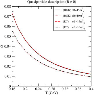
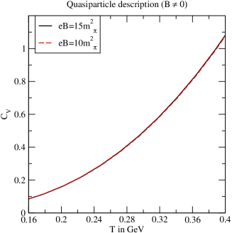
(a)	(b)

Figure 10: Variation of the Knudsen number ($\Omega$) and specific heat with temperature.

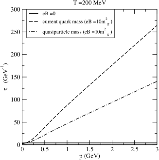
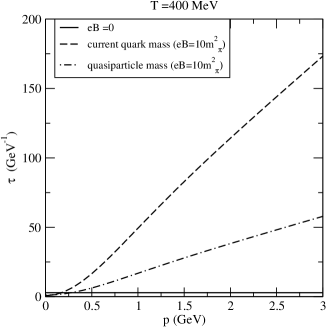
(a)	(b)

Figure 11: Variation of the relaxation time (for s quark) with momentum

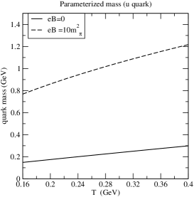
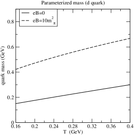
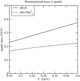
Figure 12: Variation of parameterized quark masses with temperature

Finally, we have shown in Table 2 how the quasiparticle description affects the overall effect of collision term and the subsequent modulation of strong $B$ on the charge and heat transport.

Table 2: Effect of collision term on the charge and heat transport in the absence and presence of strong magnetic field with the masses of $u$, $d$ and $s$ flavours generated in the thermal medium in background of strong $B$.

	B=0						B $\neq$ 0
Temperature	$\frac{\sigma^{BGK}}{\sigma^{RT}}$	$\frac{\kappa^{BGK}}{\kappa^{RT}}$	$\frac{\frac{\kappa}{\sigma}^{BGK}}{\frac{\kappa}{\sigma}^{RT}}$	$\frac{L_{R}^{BGK}}{L_{R}^{RT}}$	$\frac{\Omega^{BGK}}{\Omega^{RT}}$	$c_{{}_{V}}$	$\frac{\sigma^{BGK}}{\sigma^{RT}}$	$\frac{\kappa^{BGK}}{\kappa^{RT}}$	$\frac{\frac{\kappa}{\sigma}^{BGK}}{\frac{\kappa}{\sigma}^{RT}}$	$\frac{L_{R}^{BGK}}{L_{R}^{RT}}$	$\frac{\Omega^{BGK}}{\Omega^{RT}}$	$c_{V}$
Low temp.	4.06	1.76	0.43	0.42	1.68	0.20	1.68	$\approx$ 1.0	0.58	0.59	$\approx$ 1.0	0.08
(0.160 GeV)
High temp.	4.03	1.70	0.42	0.43	1.70	3.58	1.71	0.98	0.57	0.57	$\approx$1.0	1.07
(0.400 GeV)

4 Conclusion and future outlook

Our aim is to study the charge and heat transport in a strongly interacting thermal QCD medium in a background of strong homogeneous magnetic field, through the respective transport coefficients. This is a complicated proposition to start with, so we have adopted a bottom-to-top approach to handle the problem in a kinetic theory approach. First of all, we have checked how the modified BGK collision integral, unlike the commonly employed collision terms of relaxation type (RT), affects the charge and heat transport in a thermal QCD medium. This exploration is germinated due to the fact that the BGK collision term ensures conservation of particle number, momentum and energy in each collision, unlike the usually adopted collision terms of relaxation type, where the conservation of particle is ensured only on the average of a cycle. Secondly, we see that how an ambient strong magnetic field (may be produced in the peripheral events of ultrarelativistic heavy-ion collisions) modulates the collision integral, which, in turn, affects the aforesaid heat and charge transport. This exploration is motivated by the fact that the strong $B$ strongly affects the phase space, and the collision time too, which will ultimately affect the solution of the Boltzmann equation. Thirdly, instead of independent particle excitations, we see how the collective oscillation of the medium through the quasiparticle description of partons affects the occupation probability, which, in turn, affects the charge and heat transport coefficients and their derived coefficients.

The modified BGK collision integral enhances both charge and heat transport, especially more to the charge transport, compared to RT collision integral. As a consequence, the RT collision integral dominates the ratio of thermal-to-electrical conductivity (and the Lorenz number, $L_{R}$) whereas the BGK collision integral dominates the equilibration through the Knudsen number ($\Omega$), for B=0. However, in the presence of strong $B$, both electrical and thermal conductivities get amplified but the collision integrals affect on charge and heat transport differently. To be specific, BGK collision integral still dominates the charge transport whereas RT collision integral dominates the heat transport and overall strong $B$ smears the effect of collision integral. However, the large values of thermal conductivity and the reduction of the specific heat due to the dimension reduction make the equilibration factor, Knudsen number unusually large, which defies physical interpretation. Finally the quasiparticle description of the partons in the absence of strong $B$ impedes both charge and heat transport, which is reflected in the slight decrease of the conductivities. However, the quasiparticle description in strong $B$ makes the transport phenomena interesting (as seen in Table 2): i) The large values of $\sigma_{el}$ and $\kappa$ are tamed to the physically plausible values, ii) The effect of collision integral is no more sensitive to the heat transport, except $T$ is very large, and iii) the characteristic $T$-dependence of conductivities get reversed, namely $\sigma_{\rm el}$ now decreases with $T$ and the increase of $\kappa$ with $T$ is linear. As a consequence, $L_{R}$ gets bigger and increases rapidly with $T$ and becomes almost independent of $B$.

In future we are planning to explore the above study to the momentum transport and the affiliated coefficients associated to the momentum transport and investigate its implications in heavy-ion phenomenology by studying the hydrodynamic evolution of the medium along with strong $B$ produced in ultrarelativistic heavy ion collisions.

Appendix A Derivation of equation (13)

Putting the partial derivatives from (14) and (15) in (6), we get

$$-q_{i}\beta{\bf E.p}f_{\mathrm{e}q,i}(1-f_{\mathrm{e}q,i})-q_{i}\beta p_{0}\frac{{\bf E.p}}{\omega_{i}}f_{\mathrm{e}q,i}(1-f_{\mathrm{e}q,i}) = C[f],$$ (A.110)

where the BGK collision term is given by (7) as

$$C[f] = -p^{\mu}u_{\mu}\nu_{i}\left(f_{i}-n_{{}_{i}}n_{\mathrm{e}q,i}^{-1}f_{\mathrm{e}q,i}\right)$$ (A.111)

$$= -p^{\mu}u_{\mu}\nu_{i}\left(f_{i}-\frac{g_{i}\int_{p}(f_{\mathrm{e}q,i}+\delta f_{i})}{n_{\mathrm{e}q,i}}f_{\mathrm{e}q,i}\right)$$

$$= -p^{\mu}u_{\mu}\nu_{i}\left(f_{i}-\frac{(g_{i}\int_{p}f_{\mathrm{e}q,i}+g_{i}\int_{p}\delta f_{i})}{n_{\mathrm{e}q,i}}f_{\mathrm{e}q,i}\right)$$

$$= -p^{\mu}u_{\mu}\nu_{i}\left(\delta f_{i}-g_{i}n_{\mathrm{e}q,i}^{-1}f_{\mathrm{e}q,i}\int_{p}\delta f_{i}\right).$$

Now putting the value of $C[f]$ in (A.110) we get

$$2q_{i}\beta\tau_{i}~{}\frac{{\bf E.p}}{\omega_{i}}f_{\rm eq,i}\left(1-f_{\rm eq,i}\right) = \left(\delta f_{i}-g_{i}n_{\mathrm{e}q,i}^{-1}f_{\mathrm{e}q,i}\int_{p}\delta f_{i}\right)$$ (A.112)

Appendix B Derivation of the infinitesimal deviation ($\delta f_{i}^{B}$) from the local equilibrium

In order to find the deviation ($\delta f_{i}^{B}$) in the distribution function, we solve relativistic Boltzmann equation (77). Substituting the partial derivatives from (63) and (64) on the left hand side (denoted as LHS) of eqn. (77), we get

$${\rm LHS} = (p^{0}\partial_{0}T+p^{3}\partial_{3}T)\frac{\partial f_{i}^{B}}{\partial T}+(p^{\mu}u_{\nu}\partial_{\mu}p^{\nu}+p^{\mu}p^{\nu}\partial_{\mu}u_{\nu})\frac{\partial f_{i}^{B}}{\partial p^{0}}+q_{i}\left[F^{03}p_{3}\frac{\partial f_{i}^{B}}{\partial p^{0}}+F^{30}p_{0}\frac{\partial f_{i}^{B}}{\partial p^{3}}\right],$$ (B.113)

$$= \frac{p^{0}}{T}f_{\rm eq,i}^{B}(1-f_{\rm eq,i}^{B})\left[\frac{1}{T}(p^{0}\partial_{0}T+p^{3}\partial_{3}T)-\frac{1}{p^{0}}(p^{\mu}u_{\nu}\partial_{\mu}p^{\nu}+p^{\mu}p^{\nu}\partial_{\mu}u_{\nu})-2q_{i}\frac{E_{3}p_{3}}{p^{0}}\right],$$

$$= \frac{p^{0}}{T}f_{\rm eq,i}^{B}(1-f_{\rm eq,i}^{B})\left[\frac{1}{T}(p^{0}\partial_{0}T+p^{3}\partial_{3}T)-\frac{1}{p^{0}}(p^{0}\partial_{0}p^{0}+p^{3}\partial_{3}p^{0})-\frac{1}{p^{0}}(p^{0}p^{\nu}\partial_{0}u_{\nu}+p^{3}p^{\nu}\partial_{3}u_{\nu})\right.$$

$$\left.-2q_{i}\frac{E_{3}p_{3}}{p^{0}}\right]$$

$$= \frac{p^{0}}{T}f_{\rm eq,i}^{B}(1-f_{\rm eq,i}^{B})\left[\frac{1}{T}(p^{0}\partial_{0}T+p^{3}\partial_{3}T)+T\partial_{0}\left(\frac{\mu}{T}\right)+\frac{T}{p^{0}}p^{3}\partial_{3}\left(\frac{\mu}{T}\right)-\frac{1}{p^{0}}(p^{0}p^{\nu}\partial_{0}u_{\nu}+p^{3}p^{\nu}\partial_{3}u_{\nu})\right.$$

$$\left.-\frac{2q_{i}E_{3}p_{3}}{p^{0}}\right]$$

substituting $\partial_{3}\left(\frac{\mu_{i}}{T}\right)=-\frac{h_{i}^{B}}{T^{2}}\left(\partial_{3}T-\frac{T}{n^{B}_{eq,i}h_{i}^{B}}\partial_{3}P\right)$ and $\partial_{0}u_{\nu}=\frac{\nabla_{\nu}P}{n^{B}_{eq,i}h_{i}^{B}}$ from the energy momentum conservation on the left hand side (LHS) and BGK collision term on the right hand side of (77)

$$\frac{p^{0}}{T}f_{\rm eq,i}^{B}(1-f_{\rm eq,i}^{B})\left[\frac{p^{0}}{T}\partial_{0}T+\frac{(p^{0}-h_{i}^{B})}{p^{0}}\frac{p^{3}}{T}\left(\partial_{3}T-\frac{T}{n^{B}_{eq,i}h_{i}^{B}}\partial_{3}P\right)+T\partial_{0}\left(\frac{\mu}{T}\right)-\frac{p^{3}p^{\nu}}{p^{0}}\partial_{3}u_{\nu}\right.$$

$$\left.-2q_{i}\frac{E_{3}p_{3}}{p^{0}}\right]=-p^{\mu}u_{\mu}\nu_{i}^{B}\left(\delta f_{i}^{B}-g_{i}{n_{\mathrm{e}q,i}^{B}}^{-1}f_{\rm eq,i}^{B}\int\delta f_{i}^{B}\right),$$ (B.114)

which can further be solved for $\delta f_{i}^{B}$ upto first order as

$$\delta f_{i}^{B}=\delta f_{i}^{B(1)}+g_{i}{n_{\mathrm{e}q,i}^{B}}^{-1}f_{\rm eq,i}^{B}\int_{p^{\prime}}\delta f_{i}^{B(1)},$$ (B.115)

where

$$\delta f_{i}^{B(1)} = -\frac{f_{\rm eq,i}^{B}(1-f_{\rm eq,i}^{B})\tau_{i}^{B}}{T}\left[\frac{p^{0}}{T}\partial_{0}T+\frac{(p^{0}-h_{i}^{B})}{p^{0}}\frac{p^{3}}{T}\left(\partial_{3}T-\frac{T}{n_{eq,i}^{B}h_{i}^{B}}\partial_{3}P\right)+T\partial_{0}\left(\frac{\mu}{T}\right)\right.$$ (B.116)

$$\left.-\frac{p^{3}p^{\nu}}{p^{0}}\partial_{3}u_{\nu}-2q_{i}\frac{E_{3}p_{3}}{p^{0}}\right].$$

Appendix C Calculation of the quark self energy

The transverse component of the momentum in the quark propagator becomes very small $(k_{\perp}\approx 0)$, so the exponential factor ($e^{-k_{\perp}/|q_{i}B|}$) in (93) becomes unity. The quark self energy (91) in the strong magnetic field can be written as

$$\Sigma(p_{\parallel}) = \frac{2g^{2}}{3\pi^{2}}|q_{i}B|T\sum_{n}\int dk_{z}\frac{\left[\left(1+\gamma^{0}\gamma^{3}\gamma^{5}\right)\left(\gamma^{0}k_{0}-\gamma^{3}k_{z}\right)-2m_{i}\right]}{\left[k_{0}^{2}-\omega^{2}_{k}\right]\left[(p_{0}-k_{0})^{2}-\omega_{pk}^{2}\right]}$$ (B.117)

$$= \frac{2g^{2}|q_{i}B|}{3\pi^{2}}\int dk_{z}\left[(\gamma^{0}+\gamma^{3}\gamma^{5})L^{1}-(\gamma^{3}+\gamma^{0}\gamma^{5})k_{z}L^{2}\right],$$

where $\omega_{k}^{2}=k_{z}^{2}+m_{i}^{2}$, $\omega_{pk}^{2}=(p_{z}-k_{z})^{2}$ and $L^{1}$ and $L^{2}$ are the frequency sum which are given by

$$L^{1}=T\sum_{n}k_{0}~{}\frac{1}{\left[k_{0}^{2}-\omega_{k}^{2}\right]}\frac{1}{\left[(p_{0}-k_{0})^{2}-\omega_{pk}^{2}\right]}~{},$$ (B.118)

$$L^{2}=T\sum_{n}\frac{1}{\left[k_{0}^{2}-\omega_{k}^{2}\right]}\frac{1}{\left[(p_{0}-k_{0})^{2}-\omega_{pk}^{2}\right]}$$ (B.119)

after summing the above frequency sum the self energy (B.117) becomes

$$\Sigma(p_{\parallel}) = \frac{g^{2}|q_{i}B|}{3\pi^{2}}\int\frac{dk_{z}}{\omega_{k}}\left[\frac{1}{e^{\beta\omega_{k}}-1}+\frac{1}{e^{\beta\omega_{k}}+1}\right]$$ (B.120)

$$\times\left[\frac{\gamma^{0}p_{0}}{p_{\parallel}^{2}}+\frac{\gamma^{3}p_{z}}{p_{\parallel}^{2}}+\frac{\gamma^{0}\gamma^{5}p_{z}}{p_{\parallel}^{2}}+\frac{\gamma^{3}\gamma^{5}p_{0}}{p_{\parallel}^{2}}\right],$$

which after integration over $k_{z}$ simplified into

$$\Sigma(p_{\parallel})=\frac{g^{2}|q_{i}B|}{3\pi^{2}}\left[\frac{\pi T}{2m_{i}}-\ln(2)\right]\left[\frac{\gamma^{0}p_{0}}{p_{\parallel}^{2}}+\frac{\gamma^{3}p_{z}}{p_{\parallel}^{2}}+\frac{\gamma^{0}\gamma^{5}p_{z}}{p_{\parallel}^{2}}+\frac{\gamma^{3}\gamma^{5}p_{0}}{p_{\parallel}^{2}}\right].$$ (B.121)

References

- [1] K. Fukushima, Lect. Notes Phys. 871, 241 (2013).
- [2] N. Muller, J.A. Bonnet, C.S. Fisher, Phys. Rev. D 89, 094023 (2014).
- [3] D. Kharzeev, L. McLerran, H. Warringa, Nucl. Phys. A 803, 227 (2008).
- [4] V. Skokov, A. Illarionov, V. Toneev, Int. J. Mod. Phys. A 24, 5925(2009).
- [5] K. Fukushima, D.E. Kharzeev and H.J. Warringa, Phys. Rev. D78 (2008) 074033.
- [6] V.P. Gusynin, V.A. Miransky and I.A. Shovkovy, Phys. Rev. Lett. 73 (1994) 3499.
- [7] D.S. Lee, C.N. Leung and Y.J. Ng, Phys. Rev. D 55 (1997) 6504.
- [8] V.P. Gusynin and I.A. Shovkovy, Phys. Rev. D 56 (1997) 5251.
- [9] I.A. Shovkovy, Lect. Notes Phys. 871 (2013) 13.
- [10] V. Braguta, M.N. Chernodub, V.A. Goy, K. Landsteiner, A.V. Molochkov and M.I.Polikarpov, Phys. Rev. D 89 (2014) 074510.
- [11] M.N. Chernodub, A. Cortijo, A.G. Grushin, K. Landsteiner and M.A.H. Vozmediano, Phys. Rev. B 89 (2014) 081407.
- [12] D.E. Kharzeev and D.T. Son, Phys. Rev. Lett. 106 (2011).
- [13] D.E. Kharzeev, J. Liao, S.A. Voloshin and G. Wang, Prog. Part. Nucl. Phys. 88 (2016).
- [14] S. Fayazbakhsh and N. Sadooghi, Phys. Rev. D 88 (2013) 065030.
- [15] G. Basar, D. Kharzeev, D. Kharzeev and V. Skokov, Phys. Rev. Lett. 109 (2012).
- [16] K. Tuchin, Phys. Rev.C 88 (2013) 024910.
- [17] A. Bandyopadhyay, C.A. Islam and M.G. Mustafa, Phys. Rev. D 94 (2016).
- [18] N. Sadooghi and F. Taghinavaz, Annals Phys. 376 (2017) 218.
- [19] N. Sadooghi and F. Taghinavaz, Phys. Rev. D 92 (2015) 025006.
- [20] S. Fayazbakhsh, S. Sadeghian and N. Sadooghi, Phys. Rev. D 86 (2012) 085042.
- [21] S. Rath and B. K. Patra, JHEP 1712, 098 (2017).
- [22] B. Karmakar, R. Ghosh, A. Bandyopadhyay, N. Haque and M. G. Mustafa, Phys. Rev. D99, no.9,094002(2019).
- [23] K. Tuchin, Adv. High Energy Phys. 2013, 490495 (2013).
- [24] U. Gürsoy, D. Kharzeev, K. Rajagopal, Phys. Rev. C 89, 054905 (2014).
- [25] J. I. Kapusta and C. Gale, Finite Temperature Field Theory Principles and Applications (Cambridge University Press, Cambridge, United Kingdom, 2006).
- [26] S.I. Nam, Phys. Rev. D 86, 033014 (2012).
- [27] D. E. Kharzeev, Prog. Part. Nucl. Phys. 75, 133 (2014).
- [28] D. Satow, Phys. Rev. D 90, 034018 (2014).
- [29] K. Hattori and D. Satow, Phys. Rev. D 94, 114032 (2016).
- [30] P. V. Buividovich, M. N. Chernodub, D. E. Kharzeev, T. Kalaydzhyan, E. V. Luschevskaya, and M. I. Polikarpov, Phys. Rev. Lett. 105, 132001 (2010).
- [31] S. Pu, S. Y. Wu, and D. L. Yang, Phys. Rev. D 91, 025011 (2015).
- [32] M. Kurian and V. Chandra, Phys. Rev. D 96, 114026 (2017).
- [33] M. Kurian, S. Mitra, S. Ghosh and V. Chandra, Eur. Phys. J. C 79, no.2, 134 (2019).
- [34] S. Rath and B. K. Patra, Phys. Rev. D 100, no. 1, 016009 (2019).
- [35] A. Harutyunyan, D. H. Rischke, and A. Sedrakian, Phys. Rev. D 95, 114021 (2017).
- [36] S. Mitra and V. Chandra, Phys. Rev. D 96, 094003 (2017).
- [37] J. Crossno et al., Science 351, 1058 (2016).
- [38] D. Husmann, M. Lebrat, S. Häusler, J.-P. Brantut, L. Corman, T. Esslinger, Proc. Natl. Acad. Sci. 115, 8563 (2018).
- [39] X. Han, B. Liu, J. Hu, Phys. Rev. A 100, 043604 (2019).
- [40] R. Rath, S. Tripathy, B. Chatterjee, R. Sahoo, S.K. Tiwari, A. Nath, Eur. Phys. J. A 55, 125 (2019).
- [41] S. Rath and B. K. Patra, Eur. Phys. J. C 80, 747 (2020).
- [42] P. L. Bhatnagar, E. P. Gross, and M. Krook, Phys. Rev. 94, 511 (1954).
- [43] B. Schenke, M. Strickland, C. Greiner, and M. H. Thoma, Phys. Rev. D 73, 125004 (2006).
- [44] A. Hosoya and K. Kajantie, Nucl. Phys. B250, 666 (1985).
- [45] P. Braun-Munzinger and J. Stachel, J. Phys. G28, 1971 (2002).
- [46] J. Cleymans, J. Phys. G35, 044017 (2008).
- [47] A. Andronicet al., Nucl. Phys. A837, 65 (2010).
- [48] K. Fukushima and Y. Hidaka, Phys. Rev. Lett.120,162301 (2018).
- [49] K. Hattori, S. Li, D. Satow, and H.-U. Yee, Phys. Rev. D 95, 076008 (2017).
- [50] V. M. Bannur, J. High Energy Phys. 09 (2007) 046.
- [51] K. Fukushima, Phys. Lett. B 591, 277 (2004).
- [52] S. K. Ghosh, T. K. Mukherjee, M. G. Mustafa, and R. Ray, Phys. Rev. D 73, 114007 (2006).
- [53] H. Abuki and K. Fukushima, Phys. Lett. B 676, 57 (2009).
- [54] N. Su and K. Tywoniuk, Phys. Rev. Lett. 114, 161601 (2015).
- [55] W. Florkowski, R. Ryblewski, N. Su, and K. Tywoniuk, Phys. Rev. C 94, 044904 (2016).
- [56] E. Braaten and R. D. Pisarski, Phys. Rev. D 45, R1827 (1992).
- [57] A. Peshier, B. Kämpfer, and G. Soff, Phys. Rev. D 66, 094003 (2002).
- [58] J. Schwinger, Phys. Rev. 82, 664 (1951).
- [59] T. Chyi et al., Phys. Rev. D 62, 105014 (2000).
- [60] A. Ayala, J. J. Cobos-Martínez, M. Loewe, M. E. Tejeda- Yeomans, and R. Zamora, Phys. Rev. D 91, 016007 (2015).