Implications of inertial subrange scaling for stably stratified mixing

Abstract

We investigate the effects of turbulent dynamic range on active scalar mixing in stably stratified turbulence by adapting the theoretical passive scalar modelling arguments of Beguier et al. (1978) and demonstrating their usefulness through consideration of the results of direct numerical simulations of statistically stationary homogeneous stratified and sheared turbulence. By analysis of inertial and inertial-convective subrange scaling, we show that the relationship between active scalar and turbulence time scales is predicted by the ratio of the Kolmogorov and Obukhov-Corrsin constants provided mean flow parameters permit the two subrange scalings to be appropriate approximations. We use the resulting relationship between timescales to parameterise an appropriate turbulent mixing coefficient $\Gamma\equiv\chi/\epsilon$, defined here as the ratio of available potential energy ($E_{p}$) and turbulent kinetic energy ($E_{k}$) dissipation rates. With the analysis presented here, we show that $\Gamma$ can be estimated by $E_{p},E_{k}$ and a universal constant provided an appropriate Reynolds number is sufficiently high. This large Reynolds number regime appears here to occur at ${Re_{b}}\equiv\epsilon/\nu N^{2}\gtrapprox 300$ where $\nu$ is the kinematic viscosity and $N$ is the characteristic buoyancy frequency. We propose a model framework for irreversible diapycnal mixing with robust theoretical parametrisation and asymptotic behaviour in this high-${Re_{b}}$ limit.

1 Introduction

Stably stratified turbulence may be thought of as a model flow that is potentially useful for understanding aspects of geophysical and engineering processes in many regions of the oceans and atmosphere. In particular, stratified turbulence describes the relatively small-scale dynamics, in length and time, at which turbulence and irreversible mixing occurs. Interpreting and modeling such idealised flows is a primary avenue for the development and calibration of global circulation and basin-scale models, for which mixing plays a leading-order role in global energy budgets (e.g. Ferrari & Wunsch, 2009; Jayne, 2009; Gregg et al., 2018). However, even in idealised stably stratified flow configurations, parameterised modelling of mixing has emerged as a challenge due to the potential for dependence on a wide range of non-independent parameters (Ivey et al., 2018; Gregg et al., 2018; Caulfield, 2021).

Parallel to the growing recognition of the importance of modelling such small-scale processes in stratified turbulence for broader geophysical applications, stratified turbulence has been increasingly observed to exhibit certain quantitatively similar small-scale dynamics to isotropic turbulence in some parameter regimes specifically when the buoyancy Reynolds number, ${Re_{b}}$, is large enough (Gargett et al., 1981; Lindborg, 2006; de Bruyn Kops, 2015). Of course, this does not mean that stratified turbulence is equivalent in all respects, not least because stratification inevitably introduces anisotropy. We consider this parameter in more detail in the next section, but in simple terms it quantifies the dynamic range of turbulent length scales neither directly affected by large-scale stratification nor by molecular viscosity. Indeed, it is widely acknowledged that the details of the large scale, or outer, mean scale, dynamics do not strongly affect the small scale dynamics provided there is sufficient scale separation between such large and small scales. While small scale dynamics are certainly not independent of large scales (Corrsin, 1958; Durbin & Speziale, 1991), the assumption that sufficient scale separation induces statistically-independent small-scales has proven to be a valuable tool in the modelling of anisotropic turbulent flows because it allows for the application of theoretical models based on statistical symmetries, e.g., isotropy and homogeneity, to dynamic modelling.

Just to take one example, Kolmogorov-Obukhov scaling depends on the assumptions of local isotropy and homogeneity (Kolmogorov, 1941; Oboukhov, 1941a) yet it has been observed to be a good approximation for anisotropic flows provided the scale separation is sufficiently large between anisotropic turbulence scales and the dissipative viscous-diffusive scales (Champagne et al., 1970; Gargett et al., 1984; Saddoughi & Veeravalli, 1994; Shen & Warhaft, 2002). However, not all stably stratified flows exhibit sufficient scale separation for the foregoing assumption to be made (Jackson & Rehmann, 2014; de Bruyn Kops, 2015).

This phenomenology is useful because it motivates the adaptation of existing models for isotropic turbulence to stably stratified turbulence. For instance, by analysis of Obukhov-Corrsin and Kolmogorov scaling, Beguier et al. (1978) observed that the passive scalar timescale $\tau_{\phi}$ and turbulence timescale $\tau$ couple at sufficiently high Reynolds number such that they can be related by universal constants, i.e.

$$\frac{\tau_{\phi}}{\tau}\equiv\frac{E_{\phi}\epsilon}{\epsilon_{\phi}E_{k}}=\frac{\beta}{C},$$ (1)

where $E_{\phi}$ is the turbulent scalar variance, $E_{k}$ is the turbulent kinetic energy, $\epsilon_{\phi}$ and $\epsilon$ are their respective dissipation rates and $\beta,C$ are the Obukhov-Corrsin and Kolmogorov constants, respectively. The assumption that the time scale ratio is a constant is commonly applied to model scalar dissipation in Reynolds-averaged Navier-Stokes (RANS) models (e.g. Newman et al., 1981; Ristorcelli, 2006).

In modeling mixing in stratified flows, the applicability of such a universal relation is interesting due to its implications for modeling the irreversible diapycnal flux, $j_{b}$. In such models, equilibrium assumptions are typically prescribed such that the irreversible diapycnal flux is equal to a particular definition of the available potential energy dissipation rate (Osborn & Cox, 1972; Peltier & Caulfield, 2003; Caulfield, 2021) such that coupling of turbulent and scalar dynamics, as suggested by (Beguier et al., 1978), can be an insightful relation for modeling scalar dynamics.

The importance of accurately modelling such irreversible scalar fluxes in the ocean has motivated significant research of various idealised flows using an array of modelling frameworks. Perhaps most notable, estimating the irreversible flux from the scalar gradient via a turbulent diffusivity, $\kappa_{b}$, is the de facto standard approach (e.g. Ivey & Imberger, 1991; Barry et al., 2001; Maffioli & Davidson, 2016; Salehipour & Peltier, 2015), with

$$j_{b}=\kappa_{b}N^{2}$$ (2)

where $N$ is is an appropriately defined large scale buoyancy frequency. A common parametrisation of $\kappa_{b}$ has been suggested by Osborn (1980), which asserts that $\kappa_{b}$ be related to the irreversible rate of dissipation of kinetic energy via a turbulent flux coefficient $\Gamma_{b}$ such that

$$\kappa_{b}=\Gamma_{b}\epsilon/N^{2}\rightarrow\Gamma_{b}\equiv\frac{j_{b}}{\epsilon},$$ (3)

By analysis of energy equations for a simple stratified flow model at stationary conditions, Osborn (1980) suggested that $\Gamma_{b}$ be a constant $\leq 0.2$. More recently, the prescription of parameter dependence for $\Gamma_{b}$ has emerged as a necessary improvement to turbulent diffusivity models due to increasing evidence that a constant coefficient for $\Gamma_{b}$ appears not to be at all suitable. Parametrisations of $\Gamma_{b}$ in this framework have emerged to be difficult due to potential dependence on multiple parameters, which may well themselves be correlated (Caulfield, 2021), which difficulties lead to often contradictory subclosures (Monismith et al., 2018). While alternative models exists, such as mixing-length models (Odier et al., 2009; Ivey et al., 2018) and flux transport models, they have not as yet gained widespread usage in large-scale simulations.

Therefore, as the first principal objective of this research, we consider formally adapting the Beguier et al. (1978) relationship (1) to stably stratified turbulence in order to model irreversible diapycnal mixing dynamically. To evaluate this hypothesis, we consider simulations of stationary homogeneous stratified and sheared turbulence (S-HSST). S-HSST is an idealised model flow configuration that enables easy adjustment of the range of length scales (the dynamic range) available for a locally-isotropic subrange to form without changing other dimensionless flow parameters such as characteristic Froude or Richardson numbers, as defined precisely in the next section. Such a fundamental flow configuration is well suited to the evaluation of the effects of locally-isotropic scaling theories (Shih et al., 2000; Chung & Matheou, 2012). To test the hypothesis that the Beguier et al. (1978) relation can be applied to stably stratified turbulence, we perform numerical experiments of S-HSST in parameter space extremes previously inaccessible to computation. Therefore, a second principal objective of this work is to report on the characteristics of S-HSST at very large Reynolds numbers and time scales, quantitatively described in subsequent sections.

To achieve these objectives, the rest of the paper is organised as follows. In §2, we discuss a length-scale based framework for stratified and sheared turbulence and use it to derive a mixing model hypothesis based on the arguments of Beguier et al. (1978). In §3, we then describe numerical simulation experiments of homogeneous stratified and sheared turbulence (HSST). In a Reynolds number parameter-space, we then present ensemble-averaged dynamics in §4, evaluate the mixing model in §5, and finally draw our conclusions in §6.

2 Theoretical background

2.1 Parametric framework

Homogeneous sheared and stratified turbulence, HSST, is assumed to satisfy the Navier-Stokes equations subject to the non-hydrostatic Boussinesq approximation. The dimensional equations for the fluctuations relative to the planar means are

$$\frac{\partial\mathbf{u}}{\partial t}+(\mathbf{u}\cdot\nabla)\mathbf{u} =-\frac{1}{\rho_{0}}\nabla p-z\frac{\partial\mathbf{u}}{\partial x}\frac{d\bar{u}_{x}}{dz}-u_{z}\frac{d\bar{u}_{x}}{dz}\hat{\mathbf{x}}-\frac{g_{z}}{\rho_{0}}\rho\hat{\mathbf{z}}+\nu\nabla\cdot\nabla\mathbf{u},$$ (4a)

$$\frac{\partial\rho}{\partial t}+(\mathbf{u}\cdot\nabla)\rho =-z\frac{\partial\mathbf{\rho}}{\partial x}\frac{d\bar{u}_{x}}{dz}-u_{z}\frac{d\bar{\rho}}{dz}+D\nabla\cdot\nabla\rho,$$ (4b)

$$\nabla\cdot\mathbf{u} =0,$$ (4c)

where $\mathbf{u}=(u_{x},u_{y},u_{z})$ is the velocity vector in the coordinate system $(x,y,z)$ and functional dependencies have been dropped for convenience, and $\rho$ is the fluctuating density field so that the total density is

$$\rho_{t}=\rho_{0}+\overline{\rho}(z)+\rho(x,y,z,t),$$ (5)

with $\overline{\rho}(z)=zd\overline{\rho}/dz$ being the ambient density that is constant in time and has a uniform gradient antiparallel to gravitational acceleration $g_{z}$. Similarly, $\bar{u}_{z}=zd\overline{u}_{x}/dz=zS$ is the mean velocity and $S\equiv d\bar{u}_{x}/dz$ is the mean shear. The pressure decomposition is analogous to that of density and velocity so that $p$ is the fluctuating mechanical pressure relative to the temporally-constant planar mean. Internal energy and scalar transport affecting density have been combined into a single evolution equation for $\rho$ with $D$ the molecular diffusivity, $\hat{\mathbf{x}}$ and $\hat{\mathbf{z}}$ are the unit vectors in the $x$- and $z$-directions respectively, and $\nu$ is the kinematic viscosity.

2.1.1 Parametrisation

Dimensional analysis suggests that (4) can be described in terms of at least four nondimensional parameters. As we wish to interpret the dynamics in terms of the dynamic range available for various aspects of the flow, we consider parametrisation in terms of the ratios of length scales.

Here we use the convention of defining an approximate outer scale of turbulence, the large-eddy length scale, and the (viscous) Kolmogorov length scale as

$$L_{LE}\equiv E_{k}^{3/2}/\epsilon\text{ and }L_{K}\equiv(\nu^{3}/\epsilon)^{1/4},$$ (6)

where $E_{k}\equiv\langle\mathbf{u}\cdot\mathbf{u}\rangle/2$, $\epsilon\equiv\nu\langle\nabla\mathbf{u}:\nabla\mathbf{u}\rangle$ , the operator ‘$:$’ denotes the double inner product and the notation $\langle\cdot\rangle$ indicates an ensemble average.

The (buoyancy) Ozmidov length scale

$$L_{O}\equiv(\epsilon/N^{3})^{1/2}$$ (7)

defines the lower limit of length scales significantly affected by buoyancy forces, where $N$ is the (background) buoyancy frequency, defined here as

$$N^{2}\equiv-\frac{g_{z}}{\rho_{0}}\frac{d\overline{\rho}}{dz}.$$ (8)

With an explicit shear scale applied in HSST, the Corrsin length scale (Corrsin, 1958) is thought to characterise the lower limit of scales affected by shear, and is defined as

$$L_{C}\equiv(\epsilon/S^{3})^{1/2}.$$ (9)

Scales smaller than $L_{C}$ have been suggested to define a locally isotropic regime of length scales in the absence of additional smaller-scale affects of the mean-flow (Saddoughi & Veeravalli, 1994).

Given the scales defined in (6), (7) and (9), we choose to describe turbulence by the following three parameters

$${Re_{s}}\equiv\frac{\epsilon}{\nu S^{2}}=\left(\frac{L_{C}}{L_{K}}\right)^{4/3}\text{, }{Ri}\equiv\frac{N^{2}}{S^{2}}=\left(\frac{L_{C}}{L_{O}}\right)^{4/3}\text{ and }{Fr}\equiv\frac{\epsilon}{NE_{k}}=\left(\frac{L_{O}}{L_{LE}}\right)^{2/3},$$ (10)

in a fluid with a fixed Prandtl number $Pr\equiv\nu/D$ as the required fourth parameter (see Mater & Venayagamoorthy (2014) for more details on parameterisations). We choose the shear Reynolds number, $Re_{s}$, since it describes the range of length scales associated with isotropy for stationary flows with Richardson number, $Ri\leq 1$ (Mater & Venayagamoorthy, 2014). Alternative Reynolds numbers can also be useful to consider for comparison to other flow regimes, where the turbulent Reynolds number and buoyancy Reynolds numbers are defined, respectively as

$${Re}\equiv\frac{E_{k}^{2}}{\nu\epsilon}=\left(\frac{L_{LE}}{L_{K}}\right)^{4/3},\ {Re_{b}}\equiv\frac{\epsilon}{\nu N^{2}}=\left(\frac{L_{O}}{L_{K}}\right)^{4/3}.$$ (11)

In flows driven by mean shear, the energetic stationarity of the flow is thought to be characterised by $Ri$ (Jacobitz et al., 1997), measuring the scale separation between the driving shear scales and stabilising buoyancy scales. It is thought that turbulent flow configurations persist where $Ri<1$, where we distinguish between sustained turbulent flows and results derived from or interpreted in terms of linear hydrodynamic instability theory (see Zhou et al., 2017, for more discussion). Indeed, stratified turbulent simulations with prescribed shear scales have revealed that the characteristic gradient Richardson number associated with stationarity has been observed to take a Reynolds number insensitive value of

$${Ri}\approx 0.15-0.2\text{,}$$ (12)

as observed in stratified homogeneous shear flow (Shih et al., 2000; Holt et al., 1992; Portwood et al., 2019).

Furthermore, in shear-dominated flows, energy production due to shear naturally induces a strong coupling between shear and outer length scales such that the shear parameter ${S_{\ast}}$, here defined in terms of $E_{k}$ (as opposed to in terms of $q\equiv\langle\mathbf{u}\cdot\mathbf{u}\rangle$) as

$${S_{\ast}}\equiv\frac{E_{k}S}{\epsilon}=\left(\frac{L_{LE}}{L_{C}}\right)^{2/3},$$ (13)

tends to a constant between 5 and 6 at sufficiently high Reynolds numbers (Jacobitz et al., 1997; Shih et al., 2000)

However the foregoing turbulent parameters are likely insufficient to characterise active scalar dynamics, a specific point we wish to investigate in this paper. The smallest scales of the scalar are thought to be characterised by the Batchelor length scale $L_{B}$,

$$L_{B}\equiv(\nu D^{2}/\epsilon)^{1/4},$$

which coincides with $L_{K}$, at unity Prandtl number as considered in this work.

Obukhov-Corrsin similarity, which is either applicable at high Froude number or at scales smaller than those substantially affected by buoyancy, i.e. for scales smaller than $L_{O}$, implies an outer-scale scalar length scale

$$L_{OC}\equiv E_{p}^{3/2}\epsilon^{1/2}/\chi^{3/2},$$ (14)

where $E_{p}$ is the available potential energy, $\chi$ is its irreversible dissipation rate, defined in the linearly stratified limit to be

$$E_{p}\equiv\left\langle\frac{g^{2}/\rho_{0}^{2}}{2N^{2}}\rho^{2}\right\rangle\text{ and }\chi\equiv D\left\langle\frac{g^{2}/\rho_{0}^{2}}{N^{2}}|\nabla\rho|^{2}\right\rangle,$$ (15)

respectively, demonstrating that $\chi$ in this context may also be interpreted as the scaled destruction rate of buoyancy variance (Caulfield, 2021). Therefore, the range of anisotropic scales of the scalar are characterised by

$$N_{\ast}\equiv\left(\frac{L_{OC}}{L_{O}}\right)^{2/3}=\frac{NE_{p}}{\chi}.$$ (16)

Portwood et al. (2019) observed this parameter to approach unity in the high $Re_{b}$ limit for flows where $Pr=1$, and Mater & Venayagamoorthy (2014) suggests $N_{\ast}$ more descriptively parameterises turbulent mixing.

2.2 A mixing model constructed from analysis of subrange scaling

Local isotropy is a state wherein statistical symmetries of multi-point statistics, such as homogeneity, isotropy and stationarity, are present in a spatio-temporal localised region (Monin & Yaglom, 1975). In the presence of anisotropic integral scales, the conditions of local isotropy are defined, in the spatial sense, by a quasi-equilibrium range of scales that are sufficiently smaller than integral scales (Kolmogorov, 1941).

This is a prerequisite of classical inertial subrange scaling arguments (Kolmogorov, 1941; Oboukhov, 1941a; Corrsin, 1951). These state that scales within the quasi-equilibrium regime exist wherein turbulence is independent of the effects of viscosity. In shear flows, conditions for the application of local isotropy are thought to be valid at scales smaller than $L_{C}$ (Corrsin, 1958; Uberoi, 1957). Kolmogorov scaling (Kolmogorov, 1941, 1962) in the presence of anisotropic outer-scales has been revealed to coincide at scales consistent with local isotropy (Champagne et al., 1970; Saddoughi & Veeravalli, 1994). The equivalent local isotropy justification of the Kolmgorov subrange may be applied to Obukhov-Corrsin passive scalar scaling (Oboukhov, 1949; Corrsin, 1951) such that it is fit to describe an active scalar below scales affected by stratification (Monin & Yaglom, 1975, pg 391). Therefore, the spectral density of potential energy is expected to be determined by the energy dissipation rates and a wavenumber, i.e.

$$\hat{E}_{p}^{OC}(|\mathbf{k}|)=\beta\chi\epsilon^{-1/3}|\mathbf{k}|^{-5/3}f_{L}^{OC}(|\mathbf{k}|L_{C})f_{v}^{OC}(|\mathbf{k}|L_{B}),$$ (17)

where $\mathbf{k}$ is the wavenumber vector, $\beta$ is the Obukhov-Corrsin constant, the functions denoted by $f^{OC}_{v}$, $f^{OC}_{L}$ are the viscous and outer scale correction functions that are necessary without applying assumptions of local isotropy. Furthermore, according to Oboukhov (1941a), the kinetic energy spectra

$$\hat{E}_{k}^{K}(|\mathbf{k}|)=C\epsilon^{2/3}|\mathbf{k}|^{-5/3}f_{L}^{K}(|\mathbf{k}|L_{C})f_{v}^{K}(|\mathbf{k}|L_{K}),$$ (18)

where $C$ is the Kolmogorov constant, and $f^{K}_{L}$ and $f^{K}_{v}$ are the correction functions. Following the analysis of Beguier et al. (1978), by integration of (17) and (18) when $L_{C}\gg|\mathbf{k}|^{-1}\gg L_{K},L_{B}$, it is possible to obtain

$$\Pi\equiv\frac{E_{p}\epsilon}{E_{k}\chi}=\frac{\beta}{C}.$$ (19)

Therefore, the explicit relation for modeling the irreversible flux from (19) is

$$j_{b}\approx\chi\approx\frac{E_{p}\epsilon}{E_{k}\Pi},$$ (20)

with the limiting behaviour, at high Reynolds number, that $\Pi\rightarrow\beta/C$. A critical simplifying assumption in the development of (20) is that ${Fr}\geq O(1)$, though the imposition of more complex scaling relations which are thought to develop when ${Fr}\ll O(1)$ may alternatively be imposed. Indeed, more generally,

$$\Pi=\left(\frac{L_{OC}}{L_{LE}}\right)^{2/3}=\frac{N_{\ast}}{{S_{\ast}}\sqrt{{Ri}}}=N_{\ast}{Fr}\quad.$$ (21)

We stress that the assumed model spectra (17) and (18) are approximations which are difficult to observe precisely in carefully controlled experiments or simulations. Whereas these two-point scaling models are observed in flows with anistropic large scales, they are not claimed generally applicable for flows in arbitrary parameter regimes. However the sensitivity of $\Pi$ with respect to measured deviations from the model spectra is unclear a priori, a point we discuss in §4.

The relation (20) has profound implications for the calibration of a number of turbulent stratified mixing models. Generally, in gradient diffusion models,

$$\kappa_{b}\approx\frac{E_{p}}{\Pi N}{Fr},$$ (22)

while gradient diffusion subject to the model proposed by Osborn (1980) leads to

$$\Gamma_{b}\approx\Gamma\equiv\frac{\chi}{\epsilon}=\frac{E_{p}}{E_{k}\Pi}\text{ ,}$$ (23)

Combining the turbulent viscosity model of Crawford (1982) with the turbulent diffusivity model of Osborn (1980), the turbulent Prandtl number may then be expressed as

$${Pr_{t}}=\frac{1+\Gamma_{b}}{\Gamma_{b}}{Ri}=\frac{E_{k}\Pi+E_{p}}{E_{p}}{Ri}\text{ .}$$ (24)

Alternatively, the relevance of the parameter $\Pi$ to the turbulent Prandtl number model of Venayagamoorthy & Stretch (2010) implies that their key mixing parameter $\gamma$ may be expressed as

$$\gamma=\frac{\Pi}{2}\quad,$$ (25)

where $\gamma$ too has been empirically observed to assume relatively insensitive values at moderate Reynolds numbers in HSST (Venayagamoorthy & Stretch, 2006). Finally, if the objective is to construct a mixing length scale for applications in Prandtl mixing length models, such as the framework of Odier et al. (2009), where $\kappa_{b}=l_{m}^{2}S$, (20) may be equivalently expressed as

$$l_{m}=\frac{E_{p}}{\Pi N^{2}}{S_{\ast}}\text{ .}$$ (26)

3 Direct numerical simulations

In order to test the underlying hypotheses described in §2.2 leading to the irreversible mixing model embodied in (20), we must consider a stratified model flow wherein the behaviour of $\Pi$ may be evaluated as a function of dynamic range associated with isotropy. The consideration of S-HSST is justified by the emergence of a Reynolds number as the only independent non-dimensional descriptive flow parameter due to two distinct phenomenologies: (i) the coupling of the outer turbulence scales to that of the shear production mechanism such that ${S_{\ast}}\approx 5$ and (ii) the gradient Richardson number assuming a balanced apparently critical value that maintains a stationary balance of energy production and dissipation mechanisms. Both phenomenologies were discovered in DNS for this flow configuration by the investigations of Shih et al. (Shih et al., 2000, 2005) and subsequently verified more recently in a broader Reynolds number space in simulations where the Richardson number is controlled to maintain constant turbulent kinetic energy (Portwood et al., 2019). We therefore utilise the flows presented in Portwood et al. (2019) to verify the modeling framework presented in §2.2 and relevant associated consequences highlighted later in this manuscript.

3.1 Numerical method

The homogeneous stratified shear system defined by (4a) and (4b) is solved in a triply periodic domain with a Fourier pseudo-spectral method. Timestepping is performed with a fractional step method where non-linear terms are advanced with a third-order Adams-Bashforth scheme. Aliasing is treated by a sharp-spectral filter at $15/16k_{max}$, which proved to be sufficient in a-posteriori analysis. Temporal integration of the inhomogeneous shear term is handled by the integrating factor approach of Sekimoto et al. (2016). The rest of the solver is derived from the method used in Hebert & de Bruyn Kops (2006), with further details discussed therein.

The suite of simulations are designed to resolve sufficiently both the smallest and largest spatiotemporal turbulent flow scales. The streamwise extent, $L_{x}$, is is chosen to be 40 times larger than the large-eddy length scale. Because of the anisotropy of integral length scales that was observed in a limited parameter space study, the cross-stream domain length $L_{y}$ and the vertical domain length $L_{z}$ are chosen such that $L_{x}/L_{y}=2$ and $L_{x}/L_{z}=4$. A visualisation of the computational domain is featured in figure 1.

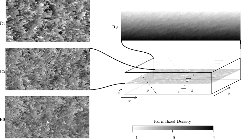
Figure 1: Illustration of simulation domain and contour plots of density. The three leftmost panels are slices of total density on an x-y slice, normalised by three times the variance of the fluctuating density in case R1; panels are shown for cases R1, R5, and R9. Note the that fluctuations decrease with Reynolds number while small-scale structure increases. Upper-right panel indicates total density normalised by minimum and maximum values for case R9, illustrating inclined large-scale structure (c.f. Chung & Matheou, 2012; Jacobitz & Moreau, 2016).

The smallest spatial scales are resolved by enforcing $k_{max}L_{K}\approx 2$, where $k_{\text{max}}$ indicates the maximum wavenumber supported by the domain discretisation when fully-resolved.

Finally, we have adopted a mass-spring-damper-like system (as similarly adopted in Overholt & Pope (1998); Rao & de Bruyn Kops (2011)), to tune the Richardson number to its stationary value by setting a constant kinetic energy target $E_{t}$. We note that this is similar to the constant power criteria as used in stationary HSST by Chung & Matheou (2012) but that here we include damping. The system is controlled by time-dependent variation of $Ri$ being required to satisfy the equation

$$c_{0}S{Ri}^{\prime}(t)+2\alpha\omega\tilde{E}_{k}^{\prime}(t)+\omega^{2}(\tilde{E}_{k}(t)-1)=0,$$ (27)

where the prime notation denotes a temporal derivative, $\tilde{E}_{k}(t)\equiv E_{k}/E_{t}$ is the normalised turbulent kinetic energy, $\omega$ is the characteristic frequency of oscillation, $\alpha$ is a dimensionless damping factor, and $c_{0}$ is a dimensionless parameter. This control system has been derived by assuming that the kinetic energy follows a second order linear system (e.g. Rao & de Bruyn Kops, 2011), and then by applying a first-order approximation to the temporal evolution of kinetic energy (c.f. Jacobitz et al., 1997)

$$\tilde{E}_{k}^{\prime}(t)\approx c_{0}S({Ri}(t)-{Ri}_{c})\hbox{\ such that \ }\tilde{E}_{k}^{\prime\prime}(t)\approx c_{0}S{Ri}^{\prime}(t).$$ (28)

The choice for the parameter $c_{0}\approx-1$ is supported by Jacobitz et al. (1997), the characteristic frequency $\omega$ is determined by the large-eddy time scale which itself is proportional to $1/S$ (Shih et al., 2000), and finally a damping coefficient $\alpha=1.5$ was found to work well.

3.2 Summary of experiments

The stationarity constraint and the emergent empirical observation that $S_{\ast}\approx 5$ lead to the natural consideration of sets of simulations which can test the effects of variation of the Reynolds number, essentially independently of the other parameters. The simulations presented here are largely equivalent to those reported in Portwood et al. (2019), though some cases have been run for longer times to ensure convergence of statistics. The various parameters of the simulations are summarised in Table 1, and some flow visualisations of the density field are shown in figure 1. Two key aspects are apparent, as noted in the caption. First, in the horizontal plane visualisations, as the Reynolds number increases, the magnitude of the density fluctuations tends to decrease, while, unsurprisingly the dynamic range of scales increases, with enhanced smaller scale structures. Second, in the vertical plane visualisation, inclined large-scale structures are apparent, consistently with the results of Chung & Matheou (2012) and Jacobitz & Moreau (2016).

	${Fr}$	${Ri}$	${Re_{b}}$	${Re_{s}}$	$N_{x}$
SHSST-R1	0.46	0.164	36	6	1024
R2	0.46	0.164	46	8	1280
R3	0.48	0.163	60	10	1536
R4	0.50	0.158	80	13	1792
R5	0.52	0.155	110	16	2048
R6	0.48	0.157	160	25	3072

	${Fr}$	${Ri}$	${Re_{b}}$	${Re_{s}}$	$N_{x}$
SHSST-R7	0.48	0.156	240	38	4096
R8	0.47	0.145	380	56	6144
R9	0.42	0.143	540	77	8192
R10	0.38	0.150	760	115	9600

Table 1: Simulation parameters. Other parameters may be inferred from definitions in the previous section. $N_{x}$ is streamwise grid points in the equispaced domain discretisation. All cases have ${Pr}\equiv\nu/D=1$.

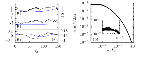
Figure 2: (a) Sample time histories of the relative kinetic energy fluctuation about the target energy and the Richardson number. Smaller fluctuations with increasing Reynolds number were observed, but generally, the kinetic energy remains within 15% of its target. (b) Longitudinal streamwise velocity spectra for case R5 sampled throughout the run period illustrating small spectral fluctuations, where the most significant fluctuations are about the smallest wavenumbers.

Time series are shown in figure 2 to illustrate convergence. Richardson numbers tend to fluctuate within about 10% of their means, at a confidence interval at least as precise as critical Richardson numbers reported by Jacobitz et al. (1997) and Shih et al. (2000). The fluctuations in the Richardson number occur at large integral timescales such that effects of $Ri^{\prime}(t)$ are small. Energetic fluctuations are more substantial than higher dimensional forcing schemes (i.e. Overholt & Pope, 1998; Rao & de Bruyn Kops, 2011) that dynamically control the flow with more granularity by accessing a broader range of turbulent length scales compared to a single mean-scale parameter as is done here. Nonetheless, energy remains approximately stationary over the large time scales of the simulations.

Recalling that the critical Richardson number is an emergent quantity from the control system defined by (27), and is not determined a priori, an increase of the critical Richardson number is not observed in these simulations as suggested by Holt et al. (1992); Shih et al. (2000), although the emergent critical value of the Richardson numbers are broadly consistent with those reported by (Shih et al., 2000). Specifically, we observe the critical gradient Richardson number which induces statistical stationarity in these flows to be approximately 0.16. Similarly, we observe ${Fr}\approx 0.5$ in all simulations, which implies ${S_{\ast}}\approx 5$, as observed in other studies (Shih et al., 2000; Jacobitz et al., 1997).

Curiously, the lowest Reynolds number to maintain stationarity robustly according to our stringent criteria corresponds approximately to case R1. Case R1 corresponds to ${Re_{b}}\approx 36$, which is consistent with critical values observed and estimated for sustained three-dimensional turbulence previously (Gibson, 1980; Shih et al., 2005; Portwood et al., 2016).

For further comparison with the flows considered by Shih et al. (2000) and Shih et al. (2005), we plot their relevant cases against the solutions presented for this research in a $Fr-Re_{b}$ parameter space as shown in figure 3. We remark that the configurations reported by Shih and co-authors in those publications feature transitional and, crucially, variable $Fr$ when $Re_{b}$ is $O(100)$. As is apparent in the figure, $Fr$ and $Re_{b}$ appear to be coupled, with approximate scaling relationship $Fr\propto Re_{b}^{1/2}$, as shown with a dashed line. Therefore, the parameterisation of mixing by $Re_{b}$ cannot be made independent of $Fr$ with the data presented in Shih et al. (2000, 2005). We note that this explanation does not rely on any argument that the simulations are inadequately resolved, either at small or large scales. Our perspective is qualitatively different from the perspective presented in Kunze et al. (2012); Gregg et al. (2018), which suggests the $Re_{b}$-sensitive regime with $Re_{b}>100$ is due to inadequate small-scale spatial resolution in the simulations. However, it is entirely plausible that the solutions analysed in Shih et. al. suffer from inadequate large scale resolution in the domain as suggested by other reports (see Kunze, 2011; Kunze et al., 2012; Gregg et al., 2018).

Therefore, disentangling the behaviour of their simulations as $Re_{b}$ varies from the effects of variation in $Fr$ is challenging, particularly when $Re_{b}$ (or $Re_{s}$) is large. It is important to remember that it was precisely for $Re_{b}\gtrsim 100$ that Shih et al. (2005) argued that the turbulent flux coefficient $\Gamma\propto Re_{b}^{-1/2}$, whereas it is entirely plausible that variable $Fr$ is playing a significant role. This figure highlights the novelty of our simulations in this particular flow configuration, which allow the isolated study of the effects of variations in Reynolds number from the influence of other non-dimensional turbulent parameters, and in particular at constant $Fr$.

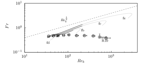
Figure 3: Flows in a $Fr-Re_{b}$ parameter space. Points indication solutions obtained in the present work. For reference, the curves indicate trajectories in parameter space of solutions for cases fz, fc, fb and fd presented in Shih et al. (2000) and Shih et al. (2005). Darker segments of those lines indicate the reporting period $St>2$ used in that research.

4 Emergent phenomena

4.1 Energetics

Just as non-dimensional parameters are emergent quantities in our simulations, so too are the partitionings of potential energy and the various components of kinetic energy. Such partitionings are significant, not least because the ratio of potential energy to kinetic energy,

$$R_{PK}\equiv E_{p}/E_{k}\;\text{ ,}$$ (29)

is a critical component to mixing models wherein Reynolds number, or ${Re_{b}}$, dependence is often omitted and the mixing is assumed to be a function of ${Ri}$ (Osborn & Cox, 1972; Schumann & Gerz, 1995; Pouquet et al., 2018). Furthermore, in ‘strongly’ stratified turbulent flow, Billant & Chomaz (2001) suggests that there should be approximate equipartition between potential and kinetic energy, i.e. $R_{PK}\approx 1$, an assumption also used by Lindborg (2006). It is important to remember that these models do not account for Reynolds number effects. Therefore, parameterisation of such energetic partitioning is an important a priori validation necessary for model evaluation.

Recalling that the kinetic energy is the same for all cases, by construction from our definition of stationarity, we observe a significant decrease in potential energy with increasing dynamic range as shown in figure 4b. In comparison, the results of Brethouwer et al. (2007), which span up to ${Re_{b}}\sim O(10)$ at much lower Froude number in homogeneous stratified turbulence, report $R_{PK}\approx 0.15$ at ${Re_{b}}={Ri}{Re_{s}}\approx 16$, noting an asymptotic trend to this value from $R_{PK}\approx 0.05$ at ${Re_{b}}\approx 0.1$. Though we observe similar values at ${Re_{s}}\approx 5$ (corresponding to ${Re_{b}}\approx 30$), higher values of ${Re_{b}}$ reveal a subsequent decline in $R_{PK}$, as suggested by Remmler & Hickel (2012). For Reynolds numbers larger than ${Re_{s}}\approx 40$ (${Re_{b}}\approx 300$), $R_{PK}$ assumes an apparently asymptotic value of $0.08$ in these simulations. This relative decrease of potential energy as a function of ${Re_{s}}$ can be observed in the domain slice visualisations of $\rho$ featured in figure 1, as there is a clear reduction in the variance of the density fluctuations. In terms of the important question concerning the modeling of mixing, and in particular parameterising the turbulent flux coefficient $\Gamma$, (23) shows that if $R_{PK}$ approaches an asymptotic value for large $Re_{s}$, $\Gamma$ can exhibit parameter dependence only if the key parameter $\Pi$ (defined in (19)) does.

Furthermore, a distinguishing characteristic of sheared stratified turbulence, relative to other stratified flows, is the absence of axisymmetry normal to gravity with the result that anisotropy must be parameterised in each dimension. Inertially-relevant anisotropy can be characterised by the variance of individual velocity vector components as they contribute to the mean turbulent kinetic energy. These velocity variances resulting from anisotropic dynamics are shown in figure 4a.

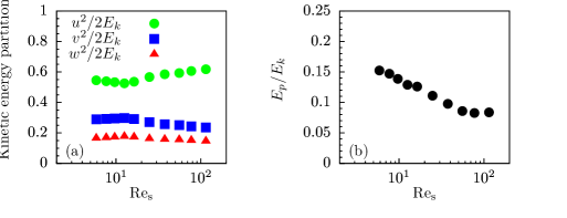
Figure 4: (a) The partitioning of kinetic energy into each velocity component where a value of $1/3$ would be expected for a statistically isotropic velocity vector. (b) The ratio of potential energy to kinetic energy, approaching asymptotic values near 0.08 for ${Re_{s}}\gtrapprox 50$.

We observe turbulent kinetic energy is dominated by streamwise velocity fluctuations with the smallest contributions coming from vertical velocity fluctuations. Notably distinct from axisymmetric flows, the horizontal components of velocity variance represent approximately 80 percent of the total contributions to kinetic energy. The cross-stream velocity variance accounts for only 30 percent of the total energy. The vertical variance, subject to exchanges to potential energy, is typically suggested to vary as a function of Froude number (Brethouwer et al., 2007). Here, the vertical variance accounts for approximately 20 percent of the total energy and we observe that it remains largely constant as a function of ${Re_{b}}$.

Perhaps surprisingly, anisotropy of velocity fluctuations increases with increasing dynamic range. That is, the streamwise velocity component becomes increasingly dominant with increasing Reynolds number, apparently at the expense of the cross-stream velocity variance. One possible interpretation is that reducing viscous effects at inertial scales as the dynamic range increases allows the flow to evolve towards an inertial equilibrium state.

4.2 Dynamics

It might be assumed that the significant energetic transitions at sufficiently high Reynolds number would be explained by accompanying clear transitions in dynamics. Here we analyse the stationary behaviour of the dynamics relevant to the kinetic and potential energy balances. The ensemble-averaged energy equations, as derived from (4), obey

$$\left\langle\frac{\partial{E_{p}}}{\partial t}\right\rangle =B-\chi\;\text{ and }$$ (30)

$$\left\langle\frac{\partial{E_{k}}}{\partial t}\right\rangle =P-B-\epsilon\;\text{ ,}$$ (31)

where the turbulent production from mean shear $P=-\langle u_{x}u_{z}\,d\bar{u}_{x}/{dz}\rangle$, the ‘buoyancy’ flux $B=\langle({g}/{\rho_{0}}){u_{z}}\rho\rangle$ have anisotropic effects on the evolution of the streamwise and vertical components of the kinetic energy $\langle u_{x}^{2}\rangle$ and $\langle u_{z}^{2}\rangle$ respectively.

Note that the left hand sides of (31), (30) reduce to approximately zero due to the stationarity constraint. Therefore, the dynamics should, at least in principle, be describable by the turbulent flux coefficient $\Gamma$ defined in terms of $\chi$ in (23), and a flux Richardson number, defined as

$${Rf}\equiv B/P\simeq\frac{\chi}{\chi+\epsilon}=\frac{\Gamma}{1+\Gamma},$$ (32)

since, if the flow actually enters an emergent stationary state the flux $B\simeq\chi$, and remembering the underlying original definition (3) $\Gamma_{b}\simeq\Gamma$. Furthermore, in this circumstance, the turbulent viscosity $\nu_{b}$ can be naturally defined as

$$\nu_{b}\equiv\frac{P}{S^{2}}\rightarrow{Pr_{t}}\equiv\frac{\nu_{b}}{\kappa_{b}}\simeq\frac{{Ri}}{{Rf}}\simeq\left(\frac{1+\Gamma}{\Gamma}\right){Ri},$$ (33)

and so we can obtain an expression consistent with (24). Henceforth, we continue to describe the evolution of energetics by $\Gamma$ defined as in (23) in recognition of the longstanding application of different definitions of the turbulent flux coefficient to estimating turbulent diffusivity and turbulent viscosity (Osborn & Cox, 1972; Crawford, 1982). Gregg et al. (2018) discuss in detail the subtleties and potential for confusion concerning different definitions for turbulent flux coefficients, and so it must always be remembered that here we concentrate on using the definition in (23), i.e. $\Gamma\equiv\chi/\epsilon$.

The ratio of terms in the energetic balance is shown in figure 5. We observe a slight decline of $\Gamma$ from $0.2$ to approximately $0.175$, as noted in Portwood et al. (2019), until ${Re_{s}}\approx 40$. However, $\Gamma$ remains approximately constant as $Re_{s}$ increases further, and in particular we do not observe the proposed ${Re_{b}}^{-1/2}$ scaling reported in a similar flow by Shih et al. (2005) for their energetic regime of ${Re_{b}}>100$. Remembering the data presented in figure 3, this is perhaps unsurprising due to the apparent correlated variation of $Fr$ and $Re_{b}$ in those simulations.

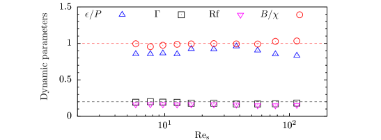
Figure 5: Relationships between various components of the potential and turbulent kinetic energy evolution equations as a function of Reynolds number. The dashed line at unity corresponds to the unimposed, but emergent, condition that $\chi\approx B$. The dashed line at 0.2 indicates the upper bound for $\Gamma$ postulated by Osborn (1980). Note that all dynamic ratios appear approximately constant as a function of Reynolds number.

Due to the condition of stationarity being imposed on the kinetic energy in our simulations, accompanying induced stationarity of the potential energy is also guaranteed, though still plotted for reference in figure 5 demonstrating that $\chi\approx B$. It is also apparent that ${Rf}\equiv B/P$ is less than $\Gamma\equiv\chi/\epsilon$, as expected.

4.3 Length scales

Since we have observed ${Fr}$ and ${Ri}$ to be essentially independent of the Reynolds number, the relatively decreasing potential energy as ${Re_{s}}$ increases for $Re_{s}\lessapprox 50$ implies that scales characteristic of the scalar should also exhibit a similar asymptotic trend. The scalar outer-scale associated with Obukhov-Corrsin similarity, $L_{OC}$ is defined in (14). In figure 6a, we plot the ratio of this outer-scale to the Ozmidov length scale $L_{O}$, as defined in (7).

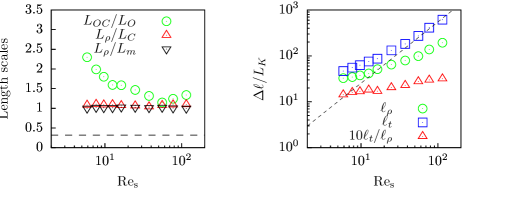
Figure 6: (a) The variation with $Re_{s}$ of the ratios of: the Obukhov-Corrsin scalar outer-scale $L_{OC}$, defined in (14), to the Ozmidov length $L_{O}$, defined in (7); the scalar mixing length $L_{\rho}$, defined in (34), to the Corrsin length scale $L_{C}$, defined in (9); and the scalar mixing length $L_{\rho}$ to the momentum mixing length $L_{m}$, also defined in (34). (b) The variation with $Re_{s}$ of: the scaling of total dynamic range, using $\Delta\ell_{t}$ and $\Delta\ell_{\rho}$, as defined in (36) and (37) respectively; and (ten times) their ratio. The expected ${Re_{s}}^{4/3}$ scaling is plotted with a dashed line, making apparent the anomalous scaling in the range of potentially isotropic scales associated with the scalar.

As $Re_{s}$ increases, this ratio decreases for $Re_{s}\lessapprox 40.$ For larger $Re_{s}$, there is some evidence that the ratio remains constant near unity, suggesting of course that $L_{OC}$ anomalously scales with $L_{O}$. This implies that the scaling $\chi\approx E_{p}N$ is valid in this high Reynolds number regime and that outer-scales of the scalar adjust to the regime associated by local isotropy, which is indeed a condition of a Obkhov-Corrsin subrange in anisotropic flows.

Length scales associated with the mixing length models suggested by Odier et al. (2009) can also be shown to remain constant in our large $Re_{s}$ regime, and indeed even for smaller $Re_{s}$. The scalar mixing length, $L_{\rho}$, and the momentum mixing length $L_{m}$, both defined by Odier et al. (2009) as

$$L_{m}\equiv\left(\frac{P}{S^{3}}\right)^{1/2},\ L_{\rho}\equiv\left(\frac{B}{N^{2}S}\right)^{1/2}\;\text{ ,}$$ (34)

are coupled via the turbulent Prandtl number ${Pr_{t}}$, which here is very close to one, since

$$L_{\rho}=L_{m}\left(\frac{BS^{2}}{PN^{2}}\right)^{1/2}=L_{m}\left(\frac{{Rf}}{Ri}\right)^{1/2}\simeq{Pr_{t}}^{-1/2}L_{m}\;\text{ .}$$ (35)

Furthermore, they coincide with the Corrsin length scale by the stationarity constraint from (31). The expected scalings $L_{\rho}\approx L_{C}$ and $L_{\rho}\approx L_{m}$ are both clearly apparent in figure 6a across a wide range of Reynolds numbers.

The decrease of $L_{OC}$ implies that the total dynamic-range associated with the scalar anomalously scales with the shear Reynolds number ${Re_{s}}$. We define the total range of dynamic scales for turbulence and the scalar as

$$\Delta\ell_{t} =(L_{L}-L_{K})\;\text{ and}$$ (36)

$$\Delta\ell_{\rho} =(L_{OC}-L_{B})\;\text{ ,}$$ (37)

respectively, and show them as a function of Reynolds number in figure 6b. With respect to the turbulence scales, after an initial small ${Re_{s}}$ transient, the range of total dynamic scales appears to increase with ${Re_{s}}^{4/3}$, as predicted by our definitions in §2.1.1. For the scalar, on the other hand, there is clearly a flatter-than-predicted scaling regime at high Reynolds number which is characteristic of the transient outer scales observed in figure 6a. Furthermore, the range of dynamics-scales associated with the scalar is significantly smaller than that of the turbulence, suggesting that if a dynamic-range threshold exists, it will not occur simultaneously for the scalar and the turbulence.

5 Implications of inertial subrange scaling

Before turning to model verification, an intermediate phenomenological test of the universality hypothesis outlined in §2.3 may be performed by analysis of the one-dimensional correlations. The one-dimensional spectra of the potential energy is expected to be determined by the energetic dissipation rates and a wavenumber, i.e. for the cross-stream spectra

$$E_{p}^{OC}(k_{y})=\beta_{1}\chi^{1}\epsilon^{-1/3}k_{y}^{-5/3}f_{L}^{OC}(k_{y}L^{O}_{yy})f_{v}^{OC}(k_{y}L_{B}).$$ (38)

In this expression, $\beta_{1}$ is the one-dimensional Obukhov-Corrsin constant. Furthermore the functions denoted by $f^{OC}_{v}$, $f^{OC}_{L}$ are the viscous and outer scale correction functions which are necessary if no implicit assumptions of local isotropy are made. The notation $L^{O}_{ij}$ indicates the outer scale of locally isotropic turbulence associated with the velocity component $i$ with respect to the direction $j$. This is ostensibly the Corrsin length scale but is inevitably anisotropic as discussed in Kaimal (1973) for the specific case of the stably stratified boundary layer.

Equivalently, according to Kolmogorov (1941) for an isotropic inertial subregime, the one-dimensional cross-stream longitudinal and streamwise transverse energy spectra are

$$E_{y}^{K}(k_{y}) =C_{1}\epsilon^{2/3}k_{y}^{-5/3}f_{L}^{K}(k_{y}L^{O}_{yy})f_{v}^{K}(k_{y}L_{K})$$ (39)

$$E_{x}^{K}(k_{y}) =C_{1}^{\prime}\epsilon^{2/3}k_{y}^{-5/3}f_{L}^{K}(k_{y}L^{O}_{xy})f_{v}^{K}(k_{y}L_{K})$$ (40)

where $C_{1}$ and $C_{1}^{\prime}$ are universal constants, and $f^{K}_{L}$ and $f^{K}_{v}$ are the correction functions. The ratio of (38) and (39) yields

$$\frac{E_{\rho}^{OC}(k_{y})}{E_{y}^{K}(k_{y})}=\frac{\beta_{1}}{C_{1}}\frac{\chi}{\epsilon}\frac{f_{L}^{OC}}{f_{L}^{K}}\frac{f_{v}^{OC}}{f_{v}^{K}}\text{ .}$$ (41)

From empirical studies of turbulence, even in the absence of the effects of stratification and shear, we expect the correction functions $f_{L}$, $f_{v}$ to be non-trivial (e.g. Muschinski & de Bruyn Kops, 2015). However, it is at least plausible that a subregime exists wherein

$$\frac{f_{L}^{OC}}{f_{L}^{K}}\approx 1\;\text{ and }\;\frac{f_{v}^{OC}}{f_{v}^{K}}\approx 1,$$ (42)

either due to sufficiently high scale separation of isotropic scales, i.e. ${Re_{s}}\gg 1$, or due to shared functional forms such that $f_{L}^{OC}=f_{L}^{K}$. Subject to either condition, it would be expected that (41) would reduce to

$$\frac{E_{\rho}^{OC}(k_{y})}{E_{y}^{K}(k_{y})}=\frac{\beta_{1}}{C_{1}}\frac{\chi}{\epsilon}\;\text{.}$$ (43)

Indeed, similar arguments would motivate the $4/3$ relation between transverse and longitudinal velocity spectra in the presence of anisotropic outer-scales such that $F_{L}^{K}(k_{y}L^{O}_{xy})\neq F_{L}^{K}(k_{y}L^{O}_{yy})$ in order to obtain

$$\frac{E_{x}^{K}(k_{y})}{E_{y}^{K}(k_{y})}=\frac{C_{1}^{\prime}}{C_{1}}=\frac{4}{3}\;\text{.}$$ (44)

The validity of the relation (43) is tested with appropriately scaled one-dimensional spectra in figure 7a, where we would expect the relation to hold in the locally isotropic wavenumber regime where $L_{C}k_{y}\sim O(1)$ (Saddoughi & Veeravalli, 1994).

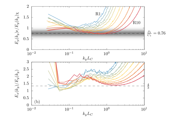
Figure 7: (a) The compensated ratio of one-dimensional energy spectra in the cross-stream direction. At high wavenumbers, the spectra lie in order of Reynolds number with R1 on the left and R10 on the right as labelled. The coexistence of Kolmogorov and Obukhov-Corrsin scaling, even when subject to non-trivial correction functions, suggests a subregime below anisotropic scales which features a plateau corresponding to the ratio $\beta_{1}/C_{1}$ of the Obukhov-Corrsin constant to the Kolmogorov constant as predicted by (43) which is expected to occur at $L_{C}k_{y}\approx 1$. The dashed line at 0.76 indicates measurements made in the stratified boundary layer by (Wyngaard & Coté, 1971) where the surrounding shaded region represents its uncertainty from reported standard deviations and the dotted line indicates an estimate of the asymptotic value of $\beta_{1}/C_{1}$ at 0.72. (b) The ratio of one-dimensional streamwise-transverse and cross-stream-longitudinal spectra, which have a predicted ratio given in (44) at high ${Re_{s}}$, expected to occur at wavenumbers a factor of ${Ri}^{-3/4}\approx 4$ greater than the locally isotropic regime shown in panel (a).

We observe a tendency for the local minima of the spectra to decrease with increasing Reynolds number. The minima for cases R8, R9 and R10 are all close to, and bounded below by 0.72, within the range of values reported for the universal constants (Sreenivasan, 1995; Sreenivasan & Kailasnath, 1996). Furthermore, in the stratified boundary layer, Wyngaard & Coté (1971) report measurements of each constant independently, in a flow configuration very similar to the one studied here, which imply $0.76\pm 0.11$, also in agreement with the results observed here.

The wavenumbers associated with this regime also tend toward smaller scales as ${Re_{s}}$ increases. In cases R8, R9 and R10, the lower-bound for this regime appears to remain fixed at approximately $k_{y}L_{C}=0.4$ as the right bound begins to increase such that the flat region of the spectra broadens. We note that this apparently asymptotic behaviour in cases R8, R9 and R10 occurs while ${Re_{s}}$ increases by a factor of two. The ratio of transverse to longitudinal one-dimensional spectra, as expressed in (44), is shown in figure 7b. We observe a similar downward trend of the locally isotropic wavenumber regime with ${Re_{s}}$, leading eventually to good agreement with the $4/3$ law for case R10.

Similarly to the data shown in figure 7a, the locally isotropic regime at higher wavenumbers becomes more consistent with the Corrsin length scale at approximately $k_{y}L_{C}\approx 2$. The misalignment of the wavenumber regimes consistent with (43) might be seen to be a consequence of the anisotropy of outer scales, as accounted for in our definitions of anisotropic length scales in $f_{L}^{K}$ and also in the observation that the outer scale of the scalar largely coincides with the Ozmidov length. Therefore, it is expected that $L_{OC}/L_{C}\sim{Ri}^{-3/4}$ and hence the wavenumber regime associated with the four-thirds relation is expected to be approximately a factor of four larger than (43), essentially as observed here.

We compare measured three dimensional potential and kinetic energy spectra to the model spectra, 18 and 17, in figures 8a,b. In both panels, a $|\mathbf{k}|^{-5/3}$ curve is plotted for reference. Our intention is to verify that the proposed spectra are approximated by our analytic model spectra at high $Re_{s}$, in the sense that we do not observe substantial systematic deviations which would otherwise indicate alternative two-point parameterisations would be more appropriate. Here we observe a trend wherein the range of scales associated with three dimensional turbulence, $|\mathbf{k}|L_{C}>1$, are approximated by the $-5/3$ power law as ${Re_{s}}$ increases. Whereas deviations from the power-law behaviour are observed at all ${Re_{s}}$, the quantitative sensitivity of the parameter $\Pi$ on deviations from the model spectra is unclear at this stage. Therefore, we next turn to evaluating the impact of Reynolds number on our key parameter $\Pi$.

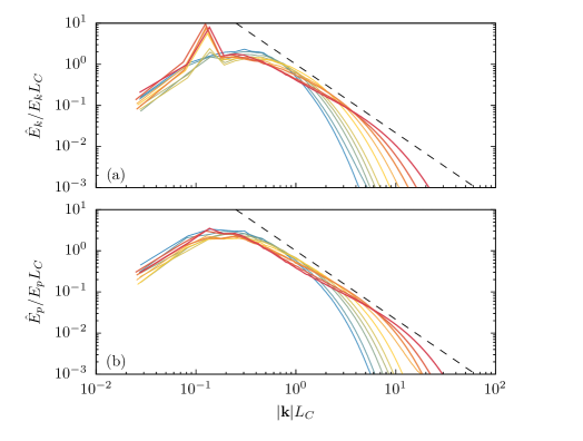
Figure 8: Three-dimensional kinetic and potential energy spectra shown in panels (a) and (b), respectively. The dashed black line indications a $-5/3$ slope, as assumed by the model spectra (18) and (17).

5.1 Model verification

In the previous section, we have presented evidence that the ratio of the potential energy spectra to a longitudinal energy spectra appears to be consistent with the underlying scaling arguments central to coexistent Kolmogorov and Obukhov-Corrsin regimes. The value of the key parameter $\Pi$ can be expressed in terms of the one-dimensional universal constants, at high Reynolds number, by

$$\Pi=\frac{\beta}{C}=\frac{6}{11}\frac{\beta_{1}}{C_{1}}.$$ (45)

For these flows, the parameter $\Pi$ should be assumed to be universal to the extent that $C$ and $\beta$ are. For reasons outlined in Sreenivasan (1991) and also observed here, measuring individual constants from a sheared flow is fundamentally problematic and furthermore measuring $\beta$ requires an accurate measurement of $\chi$, which is inherently difficult in experimental flows.

Nonetheless, estimates of the (3D) Kolmogorov and Obukhov-Corrsin constants in the literature would imply that $\Pi\approx 0.42$ (Wyngaard & Coté, 1971; Sreenivasan, 1991; Sreenivasan & Kailasnath, 1996; Yeung, 2002; de Bruyn Kops, 2015) with estimates of the individual constants typically being reported within approximately 15% of each other in the literature cited. Robust estimates of $\Pi$ from the relation (45) and empirical observations in figure 7 indicate $\Pi\approx 0.39$ which is certainly within the range of values reported in literature. We demonstrate that the important expression (45) appears to be valid within the range of uncertainty for reported values of $\beta/C$ in figure 9. We also remark that the range of $\Pi$ is small with respect to values of $\beta/C$ for the Reynolds number space considered. Such an apparently limited range of $\Pi$ has also been reported by Venayagamoorthy & Stretch (2006).

Furthermore, given the empirical observation that $L_{OC}=L_{O}$ (figure 6a) at sufficiently high Reynolds number,

$$\Pi\sim{Fr}.$$ (46)

Therefore, the stationary Froude number can be thought of as a simple consequence of the two universal constants at high Reynolds numbers, as validated in figure 9, which further implies $N_{\ast}\approx 1$, remembering (21).

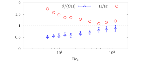
Figure 9: Verifications of relations (45) and (46) for sufficiently large ${Re_{s}}$. Error bars correspond to standard deviations associated with estimates of $C$ and $\beta$ from Wyngaard & Coté (1971). Recall that $\Pi/Fr=N_{\ast}$ from (21).

This finally suggests that the behaviour at lower Reynolds number may be parameterised by a function $f_{\Pi}$, i.e. at unity Prandtl number

$$\Pi=\frac{N_{\ast}}{{S_{\ast}}\sqrt{{Ri}}}\approx{Fr}f_{\Pi}({Re_{s}}).$$ (47)

6 Concluding remarks

Inspired by increasing evidence that high dynamic-range stratified turbulence exhibits scale-similarity as proposed by Kolmogorov (1941); Oboukhov (1949); Corrsin (1951), we have considered the formal adaptation of a passive-scalar mixing model (Beguier et al., 1978) to stratified scalar mixing. By deriving the model from scaling theories, we demonstrate how model parameters have explicit functional dependence and are Reynolds number independent, at sufficiently high Reynolds number. In order to verify our hypothesis, we have employed a model flow (i.e. S-HSST) which equilibrates such that the effects of decreasing dissipation scales, here parameterised by increasing shear Reynolds number ${Re_{s}}$ (as defined in (10)), may be investigated independently of other flow parameters.

By direct numerical simulations of S-HSST, we have shown that the outer length scales of turbulence and the active scalar become parametrically coupled such that the relationship between energetics and dissipation rates is predicted by the scaling theories of Kolmogorov and Obukhov-Corrsin similarity. Therefore, the fundamental parameter associated with this relationship, $\Pi$, as defined in (19), is the ratio (45) of the Obukhov-Corrsin constant $\beta$ and the Kolmogorov constant $C$, at sufficiently high ${Re_{s}}$, and should be considered universal to the extent that its constitutive constants are. As detailed in the context of various mixing models in §2.2, robust characterisations of $\Pi$ have strong implications on the calibration of a number of turbulence and mixing models.

This universality has profound, but still not fully-explained, implications for the turbulent flux coefficient $\Gamma$ of such steady stratified and sheared turbulence. From the expression (23), $\Gamma$ tending to a universal asymptotic value can now be understood as being due to $\Pi$ tending to a constant, which follows from the scaling theory and similarity arguments presented here, that in turn rely upon classical, and relatively well-established turbulence modelling approaches. Therefore, to ‘understand’ physically and theoretically why the empirical modeling of Osborn & Cox (1972) and Osborn (1980) works so well (with $\Gamma\sim 0.2$), the remaining interesting open question to address is why the ratio of energies $R_{PK}=E_{p}/E_{k}\simeq 0.08$ for $Re_{s}\gtrapprox 50$, as shown in figure 4.

The parameter $\Pi$ may be stated exactly as a function of $N_{\ast},{S_{\ast}},{Ri}$. However, we demonstrate that it may be effectively reduced to a function of ${Fr}$ at high Reynolds number, or a function of ${Fr}$ and ${Re_{s}}$ at low Reynolds numbers for the flows considered here. The transition of the high- and low-Reynolds number regimes is observed approximately at ${Re_{s}}\approx 40$, or ${Re_{b}}\approx 300$ at stationary Richardson number, for unity Prandtl numbers. We demonstrate that large scale characteristics of the active scalar, as parameterised by $N_{\ast}$, exhibit significant dependence on the Reynolds number for ${Re_{s}}\lessapprox 40$. The correlation between the transition point, in Reynolds number space, of the parameter $\Pi$ and $N_{\ast}$ supports the underlying assumptions of the proposed model.

A stated and significant limitation of the present study is the restriction of the model to ${Fr}\sim O(1)$ and $Pr=1$. An objective of future work is to perform a similar procedure to §2.2, except using scaling laws which account for expanded parameter regimes (for instance Lindborg, 2006; Batchelor, 1959; Kunze, 2019).

Declaration of Interests

The authors report no conflict of interest.

References

- Barry et al. (2001) Barry, M. E., Ivey, G. N., Winters, K. B. & Imberger, J. 2001 Measurements of diapycnal diffusivities in stratified fluids. J. Fluid Mech. 442, 267–291.
- Batchelor (1959) Batchelor, G. K. 1959 Small-scale variation of convected quantities like temperature in turbulent fluid. 1. general discussion and the case of small conductivity. J. Fluid Mech. 5, 113.
- Beguier et al. (1978) Beguier, C., Dekeyser, I. & Launder, B. 1978 Ratio of scalar and velocity dissipation time scales in shear flow turbulence. The Physics of Fluids 21 (3), 307–310.
- Billant & Chomaz (2001) Billant, P. & Chomaz, J.-M. 2001 Self-similarity of strongly stratified inviscid flows. Phys. Fluids 13, 1645–1651.
- Brethouwer et al. (2007) Brethouwer, G., Billant, P., Lindborg, E. & Chomaz, J.-M. 2007 Scaling analysis and simulation of strongly stratified turbulent flows. J. Fluid Mech. 585, 343–368.
- de Bruyn Kops (2015) de Bruyn Kops, S. M. 2015 Classical turbulence scaling and intermittency in stably stratified Boussinesq turbulence. J. Fluid Mech. 775, 436–463.
- Caulfield (2021) Caulfield, C. P. 2021 Layering, instabilities and mixing in turbulent stratified flows. Annu. Rev. Fluid Mech. 53, 113–145.
- Champagne et al. (1970) Champagne, F., Harris, V. & Corrsin, S. 1970 Experiments on nearly homogeneous turbulent shear flow. J. Fluid Mech. 41 (1), 81–139.
- Chung & Matheou (2012) Chung, D. & Matheou, G. 2012 Direct numerical simulation of stationary homogeneous stratified sheared turbulence. J. Fluid Mech. 696, 434–467.
- Corrsin (1951) Corrsin, S. 1951 On the spectrum of isotropic temperature fluctuations in an isotropic turbulence. J. Appl. Phys. 22, 469–472.
- Corrsin (1958) Corrsin, S. 1958 Local isotropy in turbulent shear flow. NACA Report .
- Crawford (1982) Crawford, W. R. 1982 Pacific equatorial turbulence. Journal of Physical Oceanography 12 (10), 1137–1149.
- Durbin & Speziale (1991) Durbin, P. & Speziale, C. 1991 Local anisotropy in strained turbulence at high Reynolds numbers. J. Fluids Eng. 113 (4), 707–709.
- Ferrari & Wunsch (2009) Ferrari, R. & Wunsch, C. 2009 Ocean circulation kinetic energy: reservoirs, sources and sinks. Ann. Rev. Fluid Mech. 41, 253–282.
- Gargett et al. (1984) Gargett, A., Osborn, T. & Nasmyth, P. 1984 Local isotropy and the decay of turbulence in a stratified fluid. J. Fluid Mech. 144, 231–280.
- Gargett et al. (1981) Gargett, A. E., Hendricks, P. J., Sanford, T. B., Osborn, T. R. & Williams, A. J. 1981 A composite spectrum of vertical shear in the upper ocean. J. Phys. Oceanogr. 11, 1258–1271.
- Gibson (1980) Gibson, C. H. 1980 Fossil turbulence, salinity, and vorticity turbulence in the ocean. In Marine Turbulence (ed. J. C. Nihous), pp. 221–257. Elsevier.
- Gregg et al. (2018) Gregg, M. C., D’Asaro, E. A., Riley, J. J. & Kunze, E. 2018 Mixing efficiency in the ocean. Ann. Rev. Mar. Sci. 10, 443–473.
- Hebert & de Bruyn Kops (2006) Hebert, D. A. & de Bruyn Kops, S. M. 2006 Predicting turbulence in flows with strong stable stratification. Phys. Fluids 18 (6), 1–10.
- Holt et al. (1992) Holt, S. E., Koseff, J. R. & Ferziger, J. H. 1992 A numerical study of the evolution and structure of homogeneous stably stratified sheared turbulence. J. Fluid Mech. 237, 499–539.
- Ivey et al. (2018) Ivey, G. N., Bluteau, C. E. & Jones, N. L. 2018 Quantifying diapycnal mixing in an energetic ocean. J. Geophys. Res.-Oceans 123 (1), 346–357.
- Ivey & Imberger (1991) Ivey, G. N. & Imberger, J. 1991 On the nature of turbulence in a stratified fluid. part 1: The energetics of mixing. J. Phys. Oceanogr. 21, 650–658.
- Jackson & Rehmann (2014) Jackson, P. R. & Rehmann, C. R. 2014 Experiments on Differential Scalar Mixing in Turbulence in a Sheared, Stratified Flow. J. Phys. Oceanogr. 44 (10), 2661–2680.
- Jacobitz & Moreau (2016) Jacobitz, F. & Moreau, A. 2016 Orientation of vortical steructures in turbulent stratified shear flow. In VIIIth International Symposium on Stratified Flows.
- Jacobitz et al. (1997) Jacobitz, F. G., Sarkar, S. & Van Atta, C. W. 1997 Direct numerical simulations of the turbulence evolution in a uniformly sheared and stably stratified flow. J. Fluid Mech. 342, 231–261.
- Jayne (2009) Jayne, S. R. 2009 The impact of abyssal mixing parameterizations in an ocean general circulation model. Journal of Physical Oceanography 39 (7), 1756–1775.
- Kaimal (1973) Kaimal, J. C. 1973 Turbulenece spectra, length scales and structure parameters in the stable surface layer. blm 4 (1-4), 289–309.
- Kolmogorov (1941) Kolmogorov, A. N. 1941 Local structure of turbulence in an incompressible fluid at very high Reynolds numbers. Dokl. Akad. Nauk SSSR 30, 299–303.
- Kolmogorov (1962) Kolmogorov, A. N. 1962 A refinement of previous hypotheses concerning the local structure of turbulence in a viscous incompressible fluid at high Reynolds number. J. Fluid Mech. 13, 82–85.
- Kunze (2011) Kunze, E. 2011 Fluid mixing by swimming organisms in the low-reynolds-number limit. Journal of Marine Research 69 (4-5), 591–601.
- Kunze (2019) Kunze, E. 2019 A unified model spectrum for anisotropic stratified and isotropic turbulence in the ocean and atmosphere. Journal of Physical Oceanography 49 (2), 385–407.
- Kunze et al. (2012) Kunze, E., MacKay, C., McPhee-Shaw, E. E., Morrice, K., Girton, J. B. & Terker, S. R. 2012 Turbulent mixing and exchange with interior waters on sloping boundaries. Journal of physical oceanography 42 (6), 910–927.
- Lindborg (2006) Lindborg, E. 2006 The energy cascade in a strongly stratified fluid. J. Fluid Mech. 550, 207–242.
- Maffioli & Davidson (2016) Maffioli, A. & Davidson, P. A. 2016 Dynamics of stratified turbulence decaying from a high buoyancy Reynolds number. J. Fluid Mech. 786, 210–233.
- Mater & Venayagamoorthy (2014) Mater, B. D. & Venayagamoorthy, S. K. 2014 A unifying framework for parameterizing stably stratified shear-flow turbulence. Phys. Fluids 26 (3).
- Monin & Yaglom (1975) Monin, A. S. & Yaglom, A. M. 1975 Statistical Fluid Mechanics: Mechanics of Turbulence–Volume 2. Cambridge: M.I.T. Press.
- Monismith et al. (2018) Monismith, S. G., Koseff, J. R. & White, B. L. 2018 Mixing efficiency in the presence of stratification: when is it constant? Geophys. Res. Lett. 45, 5627–5634.
- Muschinski & de Bruyn Kops (2015) Muschinski, A. & de Bruyn Kops, S. M. 2015 Investigation of Hill’s optical turbulence model by means of direct numerical simulation. J. Opt. Soc. Am. A 32 (12), 2423–2430.
- Newman et al. (1981) Newman, G., Launder, B. & Lumley, J. 1981 Modelling the behaviour of homogeneous scalar turbulence. Journal of Fluid Mechanics 111, 217–232.
- Oboukhov (1941a) Oboukhov, A. M. 1941a Spectral energy distribution in a turbulent flow. Dokl. Akad. Nauk. SSSR 32, 22–24.
- Oboukhov (1949) Oboukhov, A. M. 1949 Structure of temperature field in a turbulent flow. Izv. Akad. Nauk. SSSR, Geogr. i Geofiz 13, 58.
- Odier et al. (2009) Odier, P., Chen, J., Rivera, M. K. & Ecke, R. E. 2009 Fluid mixing in stratified gravity currents: The Prandtl mixing length. Phys. Rev. Lett. 102, 134504.
- Osborn (1980) Osborn, T. R. 1980 Estimates of the local-rate of vertical diffusion from dissipation measurements. J. Phys. Oceanogr. 10, 83–89.
- Osborn & Cox (1972) Osborn, T. R. & Cox, C. S. 1972 Oceanic fine structure. Geophysical & Astrophysical Fluid Dynamics 3 (1), 321–345.
- Overholt & Pope (1998) Overholt, M. R. & Pope, S. B. 1998 A deterministic forcing scheme for direct numerical simulations of turbulence. Comput. Fluids 27, 11–28.
- Peltier & Caulfield (2003) Peltier, W. R. & Caulfield, C. P. 2003 Mixing efficiency in stratified shear flows. Annu. Rev. Fluid Mech. 35, 135–167.
- Portwood et al. (2019) Portwood, G. D., de Bruyn Kops, S. & Caulfield, C. 2019 Asymptotic dynamics of high dynamic range stratified turbulence. Physical review letters 122 (19), 194504.
- Portwood et al. (2016) Portwood, G. D., de Bruyn Kops, S. M., Taylor, J. R., Salehipour, H. & Caulfield, C. P. 2016 Robust identification of dynamically distinct regions in stratified turbulence. J. Fluid Mech. 807, R2.
- Pouquet et al. (2018) Pouquet, A., Rosenberg, D., Marino, R. & Herbert, C. 2018 Scaling laws for mixing and dissipation in unforced rotating stratified turbulence. J. Fluid Mech. 844, 519–45.
- Rao & de Bruyn Kops (2011) Rao, K. J. & de Bruyn Kops, S. M. 2011 A mathematical framework for forcing turbulence applied to horizontally homogeneous stratified flow. Phys. Fluids 23, 065110.
- Remmler & Hickel (2012) Remmler, S. & Hickel, S. 2012 Direct and large eddy simulation of stratified turbulence. International Journal of Heat and Fluid Flow 35, 13–24.
- Ristorcelli (2006) Ristorcelli, J. R. 2006 Passive scalar mixing: Analytic study of time scale ratio, variance, and mix rate. Physics of Fluids 18 (7), 075101.
- Saddoughi & Veeravalli (1994) Saddoughi, S. G. & Veeravalli, S. V. 1994 Local isotropy in turbulence boundary layers at high Reynolds number. J. Fluid Mech. 268, 333–372.
- Salehipour & Peltier (2015) Salehipour, H. & Peltier, W. 2015 Diapycnal diffusivity, turbulent Prandtl number and mixing efficiency in Boussinesq stratified turbulence. J. Fluid Mech. 775, 464–500.
- Schumann & Gerz (1995) Schumann, U. & Gerz, T. 1995 Turbulent mixing in stably stratified shear flows. J. Appl. Meteorol. 34 (1), 33–48.
- Sekimoto et al. (2016) Sekimoto, A., Dong, S. & Jiménez, J. 2016 Direct numerical simulation of statistically stationary and homogeneous shear turbulence and its relation to other shear flows. Phys. Fluids 28 (3), 035101.
- Shen & Warhaft (2002) Shen, X. & Warhaft, Z. 2002 Longitudinal and transverse structure functions in sheared and unsheared wind-tunnel turbulence. Phys. Fluids 14 (1), 370–381.
- Shih et al. (2000) Shih, L. H., Koseff, J. R., Ferziger, J. H. & Rehmann, C. R. 2000 Scaling and parameterization of stratified homogeneous turbulent shear flow. J. Fluid Mech. 412, 1–20.
- Shih et al. (2005) Shih, L. H., Koseff, J. R., Ivey, G. N. & Ferziger, J. H. 2005 Parameterization of turbulent fluxes and scales using homogeneous sheared stably stratified turbulence simulations. J. Fluid Mech. 525, 193–214.
- Sreenivasan (1991) Sreenivasan, K. R. 1991 On local isotropy of passive scalars in turbulent shear flows. Proc. R. Soc. Lond. A 434 (1890), 165–182.
- Sreenivasan (1995) Sreenivasan, K. R. 1995 On the universality of the Kolmogorov constant. Phys. Fluids 7, 2778–84.
- Sreenivasan & Kailasnath (1996) Sreenivasan, K. R. & Kailasnath, P. 1996 The passive scalar spectrum and the Obukhov-Corrsin constant. Phys. Fluids 8, 189–96.
- Uberoi (1957) Uberoi, M. S. 1957 Equipartition of energy and local isotropy in turbulent flows. J. Appl. Phys. 28 (10), 1165–1170.
- Venayagamoorthy & Stretch (2006) Venayagamoorthy, S. K. & Stretch, D. D. 2006 Lagrangian mixing in decaying stably stratified turbulence. Journal of Fluid Mechanics 564, 197–226.
- Venayagamoorthy & Stretch (2010) Venayagamoorthy, S. K. & Stretch, D. D. 2010 On the turbulent Prandtl number in homogeneous stably stratified turbulence. J. Fluid Mech. 644, 359–369.
- Wyngaard & Coté (1971) Wyngaard, J. C. & Coté, O. R. 1971 The budgets of turbulent kinetic energy and temperature variance in the atmospheric surface layer. J. Atmost. Sci. 28 (2), 190–201.
- Yeung (2002) Yeung, P. K. 2002 Lagrangian investigations of turbulence. Annu. Rev. Fluid Mech. 34, 115–142.
- Zhou et al. (2017) Zhou, Q., Taylor, J. R., Caulfield, C. P. & Linden, P. F. 2017 Diapycnal mixing in layered stratified plane couette flow quantified in a tracer-based coordinate. J. Fluid Mech. 823, 198–229.