Identification of Methyl Isocyanate and Other Complex Organic Molecules in a Hot Molecular Core, G31.41+0.31

Abstract

G31.41+0.31 is a well known chemically rich hot molecular core (HMC). Using Band 3 observations of Atacama Large Millimeter Array (ALMA), we have analyzed the chemical and physical properties of the source. We have identified methyl isocyanate (CH₃NCO), a precursor of prebiotic molecules, towards the source. In addition to this, we have reported complex organic molecules (COMs) like methanol (CH₃OH), methanethiol (CH₃SH), and methyl formate (CH₃OCHO). Additionally, we have used transitions from molecules like HCN, HCO⁺, SiO to trace the presence of infall and outflow signatures around the star-forming region. For the COMs, we have estimated the column densities and kinetic temperatures, assuming molecular excitation under local thermodynamic equilibrium (LTE) conditions. From the estimated kinetic temperatures of certain COMs, we found that multiple temperature components may be present in the HMC environment. Comparing the obtained molecular column densities between the existing observational results toward other HMCs, it seems that the COMs are favourably produced in the hot-core environment ($\sim 100$ K or higher). Though the spectral emissions towards G31.41+0.31 are not fully resolved, we find that CH₃NCO and other COMs are possibly formed on grain/ice phase and populate the gas environment similar to other hot cores like Sgr B2, Orion KL, and G10.47+0.03, etc.

1 Introduction

Chemistry in high-mass star-forming regions (HMSFRs) is very rich, and it has a significant impact on the evolution of the Interstellar Medium (ISM) (e.g., van Dishoeck & Black et al., 1998; Tan et al., 2014). Over the years, numerous complex organic molecules (COMs) were identified in hot molecular cores (HMCs) (e.g., Herbst & van Dishoeck , 2009). Hot molecular cores are compact, hot, dense, and associated with luminous infra-red (IR) or with ultra-compact (UC) HII regions (Cesaroni et al., 2010; Bonfand et al., 2017). To date, a number of HMCs were discovered (Kurtz et al., 2000), while a limited number of circumstellar disks were found around B type stars such as the disks in Cepheus A HW2 (Patel et al., 2005), HH80-81 (Girart et al., 2018) and the disk in the late-O-type star, IRAS 13481-6124 (Kraus et al., 2010). Their dust emission has identified the majority of these disk structures. However, they are also associated with molecular emission. Complex organic molecules, CH₃CN, was observed in Cepheus A HW2 and P-V diagram of CH₃CN transitions used to understand the velocity gradient that explains gravitationally bound rotational motion.

Many complex physical processes, such as accretion, infall, and outflows are present in the earliest phase of HMSFRs during their various evolutionary stages. Therefore the chemistry of these regions is used as a diagnostic tool to examine the nature of them. Complex organic molecules are omnipresent in the HMCs and show rich chemistry. Chemistry of these regions plays an essential role, which helps trace the physical parameters associated with particular regions, such as density, temperature, and ionization rate. Since the abundances of chemical species are time dependent and collapsing time of a HMSFR is short, a comparison of observed abundance with modeling can be used to trace the chemical diversity of those region. For HMCs, both grain-surface and gas-phase processes are efficient. Various desorption mechanisms, such as thermal (active in hot core temperature) and non-thermal desorption (dominant at low temperature) processes help release the grain surface species to the gas phase.

G31.41+0.31 (hereafter G31) is an HMC that is thought to be located at a 7.9 kpc distance from the Earth (Churchwell et al., 1990). This source has a luminosity of about $\rm{\sim 3\times 10^{5}}$$L_{\odot}$. It is supposed to be heated by O and B type stars (Cesaroni et al., 2010; Beltrán et al., 2009). Previous studies (Cesaroni et al., 2011, 2017) found some hints of the existence of disk in G31.41+0.31. Osorio et al. (2009) performed detailed modeling of the SED of dust to obtain the physical parameters of the star and the core. Using these parameters, they estimated the ammonia emission and compared it with the VLA observation having a sub-arcsec resolution of G31. They obtained the mass of the central star $\sim$ 20-25 M_⊙ and significantly higher mass (1400-1800 M_⊙) of the envelope by considering envelope size, R_env = 30000 AU. Recently, Beltrán et al. (2018) observed G31 with ALMA at $1.4$ mm resolved G31 into two cores, namely main and NE. They observed the physical properties such as accelerating infall, rotational spin up, red-shifted absorption, and possible outflow directions associated with this source. The UC HII region is situated at the North-East side of G31 and separated by $\sim 5^{{}^{\prime\prime}}$ from the main core (Cesaroni et al., 2010). The main core’s estimated mass is 120 M_⊙, which is based on old distance 7.9 kpc (Beltrán et al., 2018). However, new parallax measurement suggests that G31 is located at a distance of 3.7 kpc. Therefore the luminosity of the source would be $\rm{\sim 4\times 10^{4}}$$L_{\odot}$ and estimated mass of the main core ($M_{c}$) of G31 is $\sim$ 26 M_⊙ (Ried et al., 2019; Estalella et al., 2019; Beltrán et al., 2019). However, this estimation should be considered the lower limit because high angular resolution might have filtered spatially extended emission (Beltrán et al., 2019).

A wide variety of species (around $70$) were already identified in G31. The simplest form of sugar, glycolaldehyde (HOCH₂CHO), was observed in G31 with IRAM PdBI at $1.4$, $2.1$, and $2.9$ mm observations (Beltrán et al., 2009). This is the earliest evidence of the presence of sugar outside our Galactic center. A large number of COMs such as methanol (CH₃OH), methyl cyanide (CH₃CN), ethanol (C₂H₅OH), ethyl cyanide (C₂H₅CN), methyl formate (CH₃OCHO), dimethyl ether (CH₃OCH₃), ethylene glycol (CH₂OH)₂, and acetone (CH₃COCH₃) had already been identified in G31 by using both single dish (IRAM 30m, GBT) and Submillimeter Array (SMA) observations (Rivilla et al., 2017; Isokoski, Bottinelli & van Dishoeck., 2013, and references therein).

The presence of a large number of COMs, including branched chain molecule might be an indication of the existence of prebiotic molecules and essential building blocks of life in space (Belloche et al., 2014; Chakrabarti et al., 2015; Majumdar et al., 2015; Sil et al., 2018; Sahu et al., 2020). Goesmann et al. (2015) detected various COMs (e.g., methyl isocyanate, formamide, glycolaldehyde, ethylamine etc.) in a Jupiter family comet, 67P/Churyumov-Gerasimenko (67P/C-G). Among them, methyl isocyanate (CH₃NCO) was found to be relatively abundant as compared to other observed COMs. However, Altwegg et al. (2017) reported the resulting CH₃NCO abundance as an upper limit. The presence of CH₃NCO in space is supposed to be important because of its peptide-like bond. Detection of CH₃NCO was first claimed by Halfen et al. (2015) in a massive hot molecular core, Sgr B2. It was also detected in Orion KL (Cernicharo et al., 2016). It has recently been observed in G10.47+0.03 (Gorai et al., 2020). Here, in G31, we have identified some transitions of this species.

Methanethiol ($\rm{CH_{3}SH}$) is a sulfur analog of methanol, where the S atom is replaced by an O atom. To date, this is the only complex sulfur-bearing species (having 6 atoms) which has been firmly detected in the ISM. Tentative identification of higher-order thiols, ethanethiol ($\rm{C_{2}H_{5}SH}$) has been reported in Sgr B2N (Müller et al., 2016). Identification of $\rm{CH_{3}SH}$ was also reported toward the Galactic center (Linke et al., 1979; Müller et al., 2016), Orion KL (Kolesniková et al., 2014) and chemically rich massive hot core, G327.3-6 (Gibb et al., 2000) and 67P/C-G comet (Calmonte et al., 2016).

In this work, we present the interferometric (ALMA archival data) observation towards G31. We report first detection of CH₃NCO and CH₃SH in G31 and discuss the kinematics associated with this HMC. We also discuss the chemistry of other complex species in this source. The remainder of this paper is summarized as follows. In Section 2, we describe observational details and data reduction processes. All results are presented and discussed in Section 3 and Section 4 respectively. Finally, we draw our conclusion in Section 5.

2 ALMA archival data

In this paper, we used Atacama Large Millimeter/submillimeter Array (ALMA) cycle 3 archival data (#2015.1.01193.S) to study COMs in G31. The observation was performed during June, 2016 using forty 12 m antennas. The shortest and the longest baseline was $15$ m, and $783.0$ m, respectively, and synthesized beam size was $\sim$ 1.1 ^′′. Four spectral windows (86.559-87.028 GHz, 88.479-88.947 GHz, 98.977-99.211 GHz, and 101.076-101.545 GHz) of width $~{}0.47$ GHz was set up to observe the target source, G31; phase center was $\alpha$(J2000) = 18^h47^m34.309^s, $\delta$ =-1^o12^′46.00^′′. The flux calibrator was Titan, the phase calibrator was J1824+0119, and the bandpass calibrator was J1751+0939. The data cube has a spectral resolution of 244 kHz ($\sim$0.84 km s^-1) with a synthesized beam of $\sim$ $\rm{1.19^{{}^{\prime\prime}}\times 0.98^{{}^{\prime\prime}}}$ having position angle (PA) $\sim$ 76^o. The systematic velocity of the source is known to be $\sim$ $97$ km s^-1 (Cesaroni et al., 2010; Rivilla et al., 2017). Image analysis was done using CASA 4.7.2 software (McMullin et al., 2007). Implementing the first-order baseline fit and by using ‘uvcontsub’ command available in the CASA program, we separated each spectral window into two data: continuum and line emission. The identification of lines of all the observed species presented in this paper is carried out using CASSIS (This software was developed by IRAP-UPS/CNRS, http://cassis.irap.omp.eu) together with the spectroscopic database ‘Cologne Database for Molecular Spectroscopy’ (CDMS, Müller et al., 2001, 2005) and Jet Propulsion Laboratory (JPL, Pickett et al., 1998) database.

3 Results

3.1 Continuum emission and $\rm{H_{2}}$ column density estimation

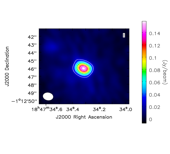
Figure 1: Continuum map of G31 obtained with ALMA at $94$ GHz. Contour levels start at 4$\sigma$ (1$\sigma$=7 mJy/beam) and steps are in 3$\sigma$. Ellipse at the below left corner of the image shows the synthesized beam ($\rm{1.19^{\prime\prime}\times 0.98^{\prime\prime}}$) with PA=76.83^o.

The continuum image of G31 at $94.3$ GHz is shown in Figure 1. The synthesized beam size of the continuum is $\rm{1.19^{{}^{\prime\prime}}\times 0.98^{{}^{\prime\prime}}}$ with PA $\sim$76$\degree$. Using two-dimensional Gaussian fitting over the dust continuum emission, we obtained the deconvolved size of G31 $\sim 0.90^{\prime\prime}\times 0.68^{\prime\prime}$ .

Assuming the distance to the source $7.9$ kpc, we obtained a source size $\sim 7110\times 5372$ AU. This source size changes to $3330\times 2516$ AU, while $\sim 3.7$ kpc distance is used.

Beltrán et al. (2018) observed G31 with an angular resolution of 0.22^′′ and found the continuum brightness temperature $\sim$132 K, which is comparable to the dust temperature ($\sim 150$ K). This suggests that the dust continuum emission observed at $217$ GHz is optically thick. Rivilla et al. (2017) also observed that dust opacity is high ($\tau$ = 2.6) at 220 GHz.

We have observed peak intensity of the continuum is $\sim$158 mJy/beam which corresponds to a brightness temperature $18$ K (using Rayleigh-Jeans approximation, 1 Jy/beam $\equiv$ 118 K). This estimation is much smaller than the assumed dust temperature of 150 K, this indicates a small optical depth ($\rm{\tau_{\nu}}$) $\sim$ 0.12 (using $T_{mb}=T_{d}(1-exp(-\tau_{\nu}))$.

It should be noted that in our observation, the source was not resolved or at best marginally resolved; therefore, the estimated brightness temperature could be underestimated.. After adding the beam dilution correction for the unresolved source, the brightness temperature is estimated to be $\sim$36 K. Considering this value of brightness temperature; dust emission remains optically thin ($\tau_{\nu}\sim 0.24$). Due to the collapsing envelope, we can expect higher density and temperature toward the inner region than the outer envelope of this source. Since dust density is higher towards the inner region, opacity would be higher, as observed by Beltrán et al. (2018). It may reduce the true line intensity of the observed transitions. However, due to the lower angular resolution, our present data would not provide further details about the dust opacity of the whole region of G31.

Assuming the dust continuum to be optically thin, flux density can be written as,

$$S_{\nu}^{beam}=\Omega_{beam}\tau_{\nu}B_{\nu}(T_{d}),$$ (1)

where $\Omega_{beam}$=$\frac{\pi}{4ln2}$ $\times\theta_{major}\times\theta_{minor}$ is solid angle of the synthesized beam, S${}_{\nu}^{beam}$ is the peak flux density measured in unit of mJy/beam, $\tau_{\nu}$ is optical depth, and $\rm{T_{d}}$ is dust temperature and $\rm{B_{\nu}(T_{d})}$ is Planck function (Whittet , 1992). Optical depth can be expressed as,

$$\tau_{\nu}=\rho_{d}\kappa_{\nu}L,$$ (2)

where $\rho_{d}$ is the mass density of dust, $\kappa_{\nu}$ is the mass absorption coefficient, and L is the path length. Using the dust to gas mass ratio ($Z$), the mass density of the dust can be written as,

$$\rho_{d}=Z\mu_{H}\rho_{H_{2}}=2Z{\mu_{H}}N_{H_{2}}m_{H}/L,$$ (3)

where $\rho_{H_{2}}$ is the mass density of hydrogen molecule, $\rm{N_{H_{2}}}$ is the column density of hydrogen, $\rm{m_{H}}$ is the hydrogen mass, and $\rm{\mu_{H}}$ is the mean atomic mass per hydrogen atom. Here, we used $Z=0.01$, $\mu_{H}=1.41$ (Cox et al., 2000), and dust temperature 150 K. Two dimensional Gaussian fitting of the continuum yields a peak intensity (S${}_{\nu}^{beam}$) of dust continuum of 158.4 mJy/beam and integrated flux (F_ν) of 242.4 mJy. RMS noise of the continuum map was found to be $5$ mJy/beam. From the above equations column density of molecular hydrogen can be written as,

$$N_{H_{2}}=\frac{S_{\nu}^{beam}/\Omega_{beam}}{2\kappa_{\nu}B_{\nu}(T_{d})Z\mu_{H}m_{H}}.$$ (4)

According to the interpolation of the data presented in Ossenkopf & Henning (1994), we estimated the mass absorption coefficient. By considering a thin ice condition, here, we obtained the mass absorption coefficient at 94 GHz ($3187.90$ micron) $\sim 0.176$ cm²/g. By using equation 4, total hydrogen column density of G31 source is $\sim{\rm 1.53\times 10^{25}}$ cm^-2.

3.2 Line analysis, molecular emission and spectral fitting

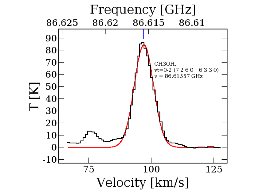
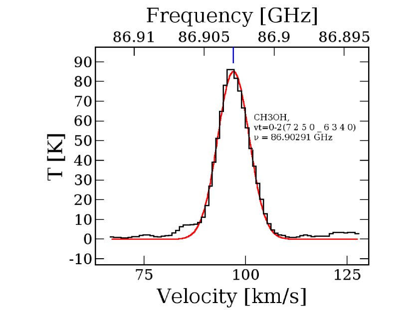
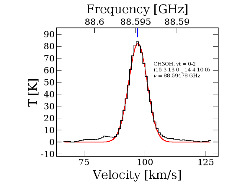
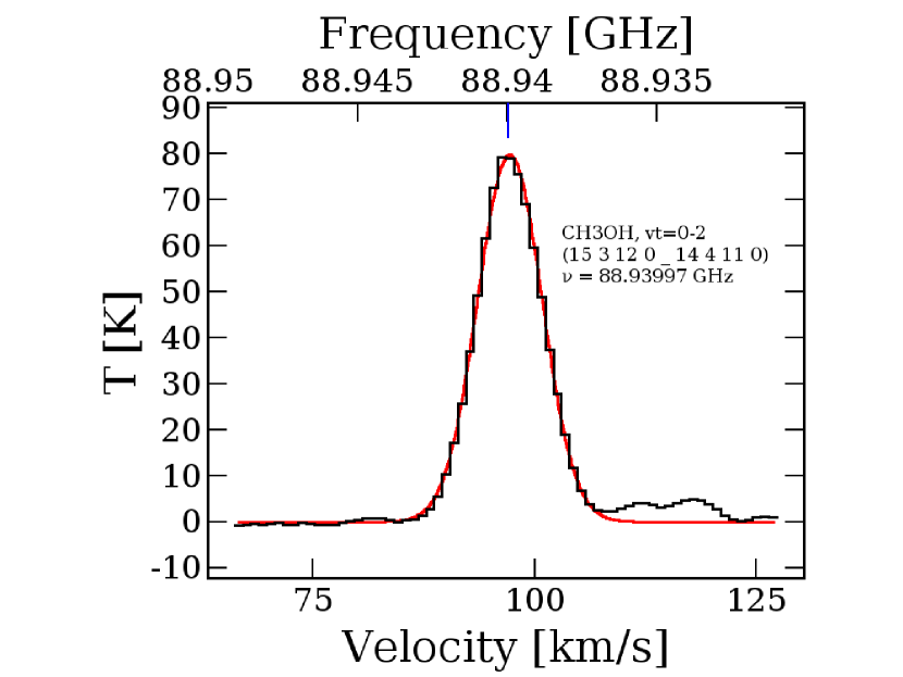
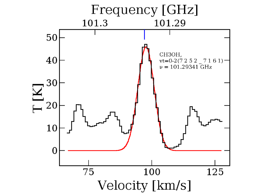
Figure 11: Black line represents observed emission spectra of methanol (CH₃OH) and red line represents a Gaussian profile fitted to the observed spectra.

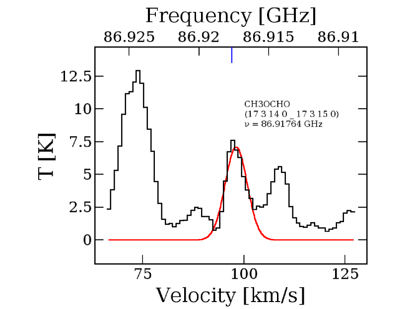
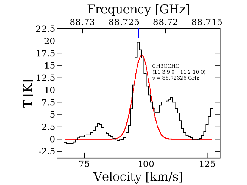
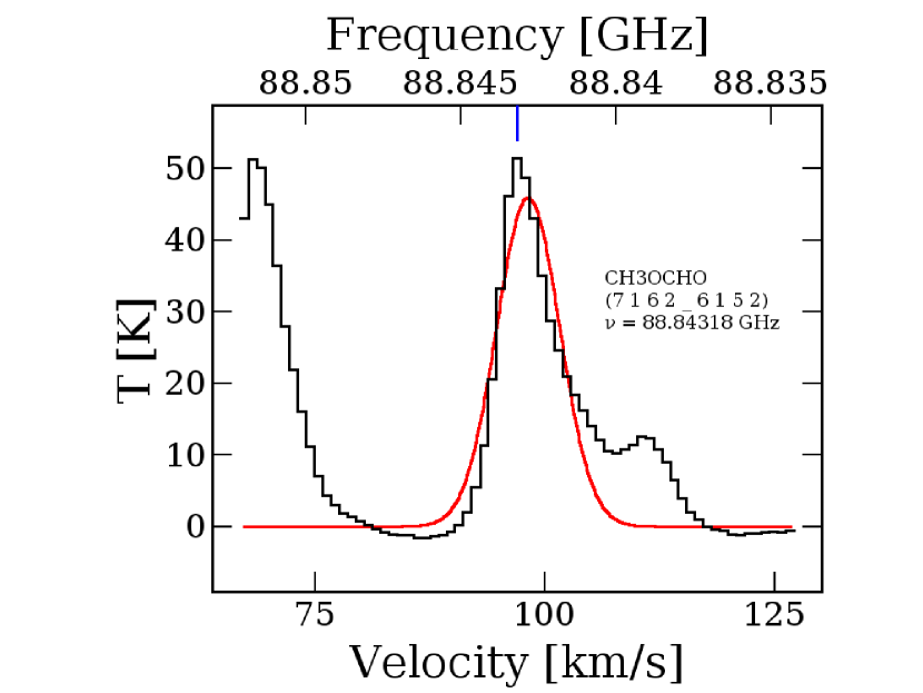
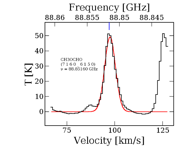
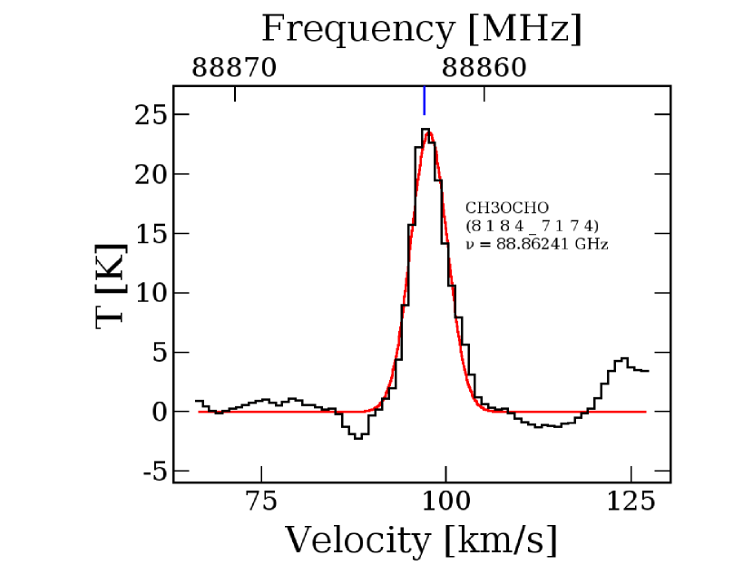
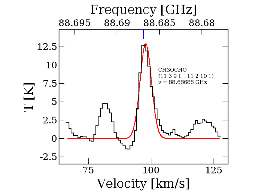
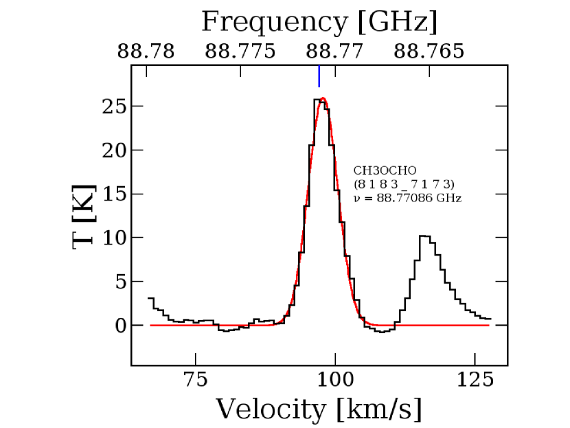
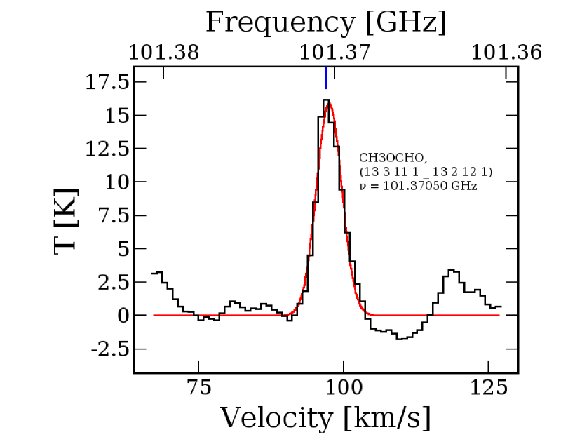
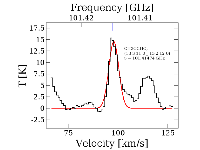
Figure 12: Black line represents observed emission spectra of methyl formate (CH₃OCHO) and red line represents a Gaussian profile fitted to the observed spectra. $\rm{11_{39}-11_{2,10}(A)}$ transition may blend with some other molecular transition.

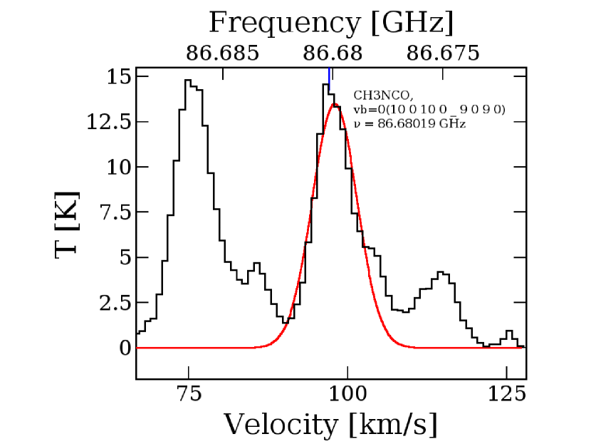
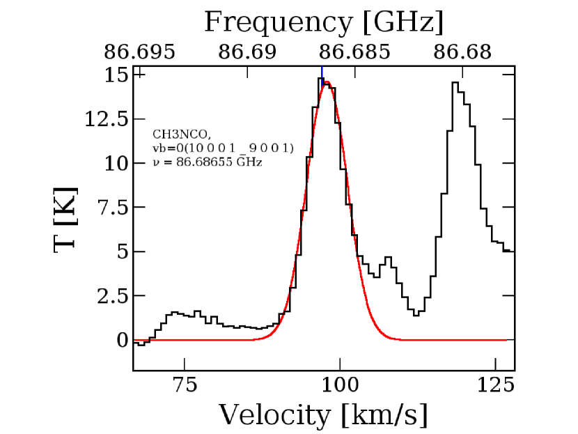
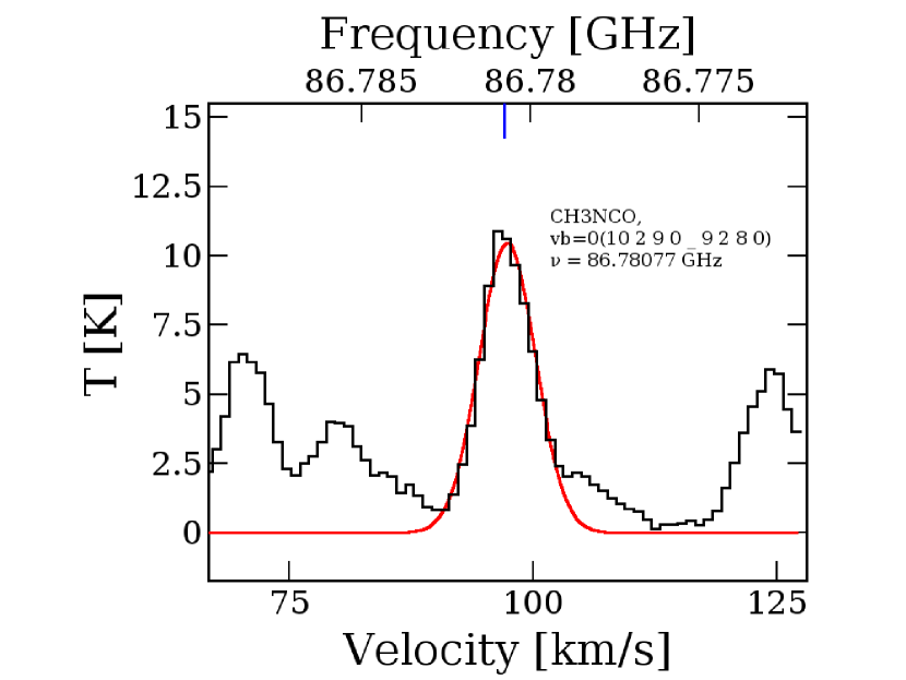
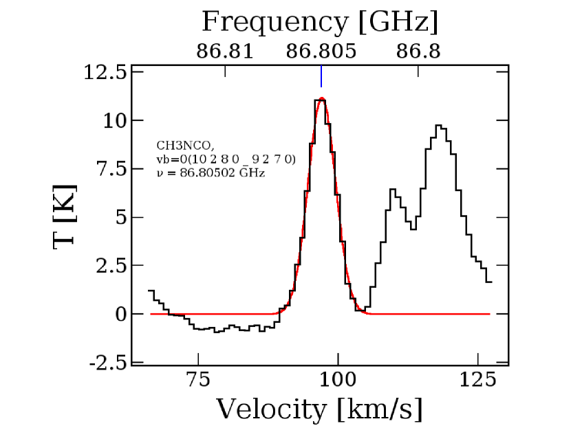
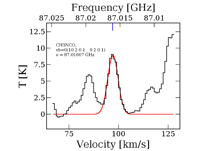
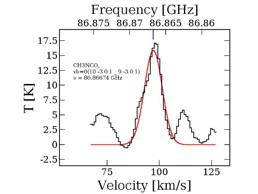
Figure 13: Black line represents observed emission spectra of methyl isocyanate (CH₃NCO) and red line represents a Gaussian profile fitted to the observed spectra. $\rm{10_{-30}-9_{-30}}$ transition may strongly blend with some other molecular transitions.

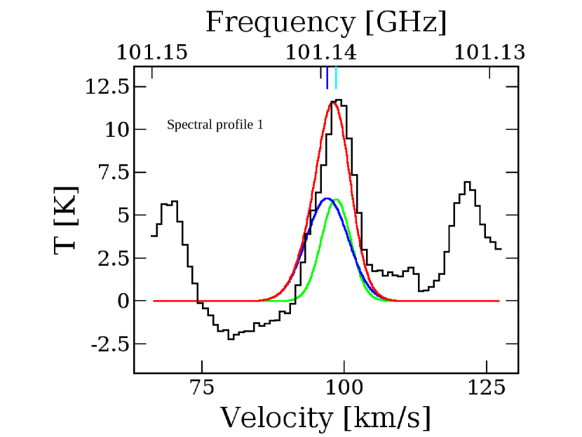
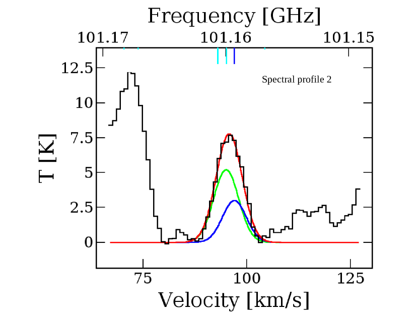
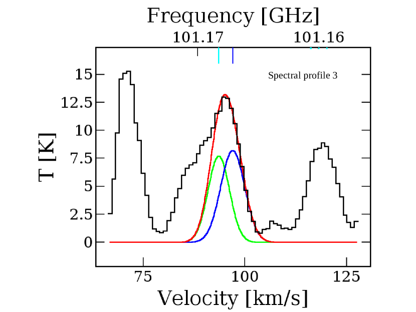
Figure 14: Black line represents observed emission spectra of methanethiol (CH₃SH) and red line represents the resultant Gaussian profile of multiple Gaussian components fitted to the observed spectra. In the left panel, blue profile represent the 101.13915 GHz line and green line represent the 101.13965 GHz transition. In the middle panel, though we observe four transitions, we consider two Gaussian components one (blue profile) for 101.15933 GHz and another one (green profile) for other three multiplets (101.15999 GHz, 101.16066 GHz, and 101.16069 GHz). In the right panel, blue and green lines represent 101.16715 GHz and 101.16830 GHz transitions respectively.

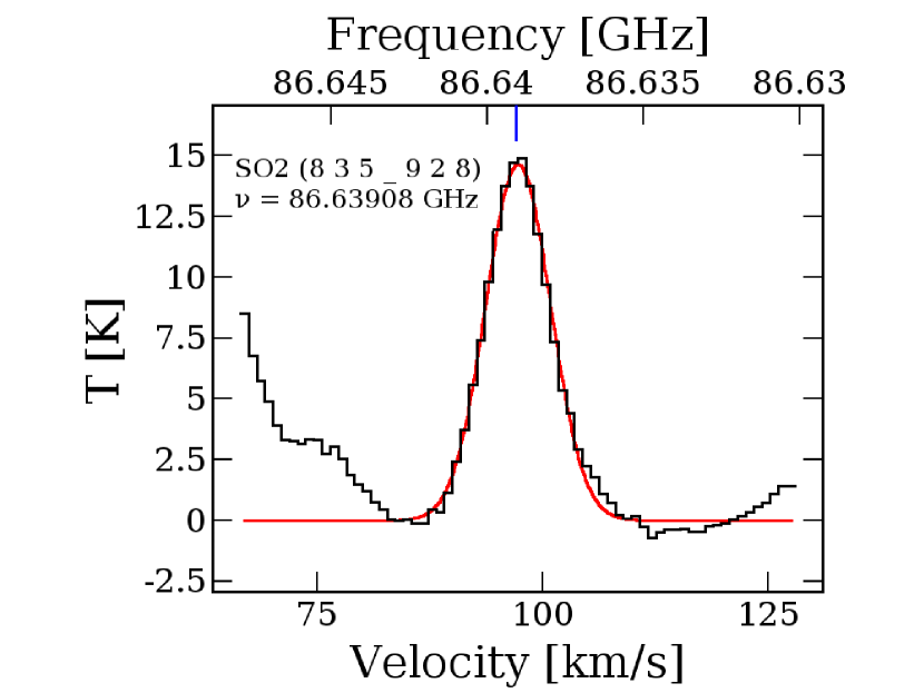
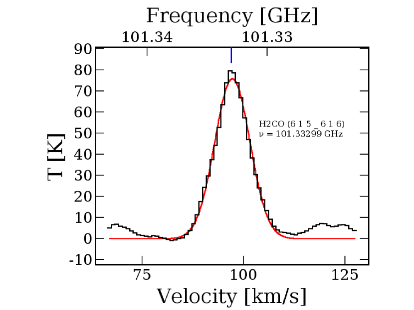
Figure 15: Black line represents observed emission spectra of SO₂, and H₂CO and red line represents a Gaussian profile fitted to the observed spectra.

Observed spectra are obtained within the circular region having a diameter of 1.1^′′ centered at RA (J2000) = 18^h47^m34.309^s, Dec (J2000) =-1^o12^′46.00^′′. Line parameters of all the observed transitions are obtained using a single Gaussian fit. From fitting, we have estimated the line width (FWHM), LSR velocity, and the integrated intensity. All the line parameters of observed molecules such as molecular transitions (quantum numbers) along with their rest frequency ($\nu$), line width (FWHM, $\Delta V$), integrated intensity ($\rm{\int T_{mb}dV}$), upper state energy (E_u), $\rm{V_{LSR}}$, and transition line intensity (S$\mu^{2}$, where S is the transition line strength and $\mu$ is the dipole moment) are presented in Table 1. Overall, we have observed a broad line width ($\geq$ 5 km s^-1) and all lines are at the center around the systematic velocity of the source ($\rm{\sim 97\ km\ s^{-1}}$) (see Table 1). In the Appendix, we have presented observed and Gaussian fitted spectra (see Figures 11-15).

Figure 2: Observed spectra of (a) $\rm{H^{13}CO^{+}}$ (inverse P-Cygni) and (b) HCN towards the dust continuum peak. 86.631847 GHz transition of HCN is used to set the velocity scale. Other two lines (green dashed) are plotted in the same figure by taking the difference in frequency between the transitions which corresponds to have velocity shift by $\sim$ 7 $\rm{km\ s^{-1}}$. for transition 88.63393 and $\sim$ 5 $\rm{km\ s^{-1}}$ for 88.63041 GHz. Bold dashed green line shows the systematic velocity ($\rm{V_{LSR}}$) of the source $\rm{\sim 97\ km\ s^{-1}}$.

3.2.1 Simple Molecules

We have observed SO₂ ($86.63908$ GHz) and H₂CO ($101.33299$ GHz) in G31. We have also identified some simple molecules such as HCN, H¹³CO⁺, and SiO, which are widely used to trace various physical processes of star-forming regions. The observed spectral profile of H¹³CO⁺ shows red-shifted absorption, which is shown in Figure 2a. This is a signature of inverse P-Cygni profile. This suggests that the source has an infall nature. Observed emission of SiO and HCN traces the outflows in this source.

Figure 2b shows the observed spectral profile of HCN. Here, we have identified three hyperfine transitions of HCN (F = 1$\rightarrow$1, 2$\rightarrow$1, and 1$\rightarrow$0 hyperfine components of the J=1$\rightarrow$0 transition, see Table 2). Three hyperfine transitions of HCN are appeared in absorption and blended together. These three absorption lines together resulting in a broad feature. HCN traces the outflow associated with the source. The observed transitions of both HCN and H¹³CO⁺ are found to be optically thick.

Here, we have also detected one transition of SiO at 86.84696 GHz (J=2$\rightarrow$1). SiO shows the absorption feature towards the center of the dust continuum and emission profile at all other positions. (Beltrán et al., 2018) also observed similar spectral feature of SiO (5-4, 217.10498 GHz). SiO traces outflows associated with this source.

3.2.2 Complex Organic Molecules

We have observed numerous COMs that were previously reported in G31 (e.g., Rivilla et al., 2017, and references therein). Additionally, for the first time in this source, we are reporting the detection of two new molecules, methyl isocyanate (CH₃NCO) and methanethiol (CH₃SH). Altogether, we have identified six transitions of CH₃NCO with the ground vibrational state ($v_{b}=0$) and one transition with $v_{b}=1$. Among the six transitions of CH₃NCO, one transition (86.86674 GHz) is blended with ethylene glycol (confirmed from LTE modeling).

We have identified three different peaks of CH₃SH, where each peak contains multiple transitions. These transitions are reported in Table 1. We are unable to separate these observed transitions. Because of closely spaced transitions, it is difficult to distinguish two or more different transitions from a single observed peak of CH₃SH. Thus, to obtain the observed line parameters of CH₃SH transitions, we have fitted multiple Gaussian components to the observed spectra. For multiple Gaussian fitting, we have used fixed values of velocity separation and expected line intensity ratio. Only FWHM is kept as a free parameter. This method works well in the observed spectral profile 1 and 3 around 101.139 GHz and 101.167 GHz of CH₃SH, where there are two transitions around each profile (see Table 1). Two-component Gaussian fitting corresponding to the two transitions are used to fit those spectral profiles (see Table 1 and Figure 14). However, this method does not work well for spectral profile 2, around 101.159 GHz, where four transitions are present. The four transitions can be classified into two classes based on their expected peak intensity (equivalent to S$\mu^{2}$) and E_up. The expected intensity ratio between these four transitions is 1:0.58:0.58:0.58. We have used two-component Gaussian fitting corresponding to the two classes of transitions, one for 101.15933 GHz (S$\mu^{2}$ =4.96, E_up=31.26 K) transition and another component for the other three transitions, 101.15999 GHz, 101.16066 GHz, 101.16069 GHz (S$\mu^{2}$ = 2.90, E_up = 52.55 K) around 101.159 GHz line profile. For the fitting, we have used 1:1.74 (1.74 is the sum of intensity of three transitions) intensity ratio for these two components. Therefore, resultant Gaussian corresponding to the three transitions can be obtained via this method; as these transitions are equally intense and have similar excitation temperature, the area under Gaussian can be divided by three to get the contribution from each transition multiplets. We have used only one transition from these multiplets for the rotation diagram of CH₃SH since the integrated area of all these three transitions are the same and have similar upper state energy (E_up). Therefore, these fitting results are used meaningfully to estimate rotational temperature using the rotation diagram method. Obtained line parameters are further used in the rotation diagram of CH₃SH. For the rotation diagram of CH₃SH, we use 101.13915 GHz, 101.13965 GHz, 101.15933 GHz, 101.1599 GHz, 101.16715 GHz, and 101.16830 GHz transitions. Gaussian fits of CH₃SH observed spectra are provided in Figure 14.

Figure 3: The integrated intensity distribution (color) of (a) SO₂, (b) H₂CO, (c) CH₃OH, (d) CH₃OCHO, (e) CH₃SH, (f) and CH₃NCO lines overlaid of the 3.1 mm continuum emission (black contours) is shown. Contour levels are at 20%, 40%, 60 %, and 80% of the peak flux. The synthesized beam is shown in the lower left-hand corner of each figure.

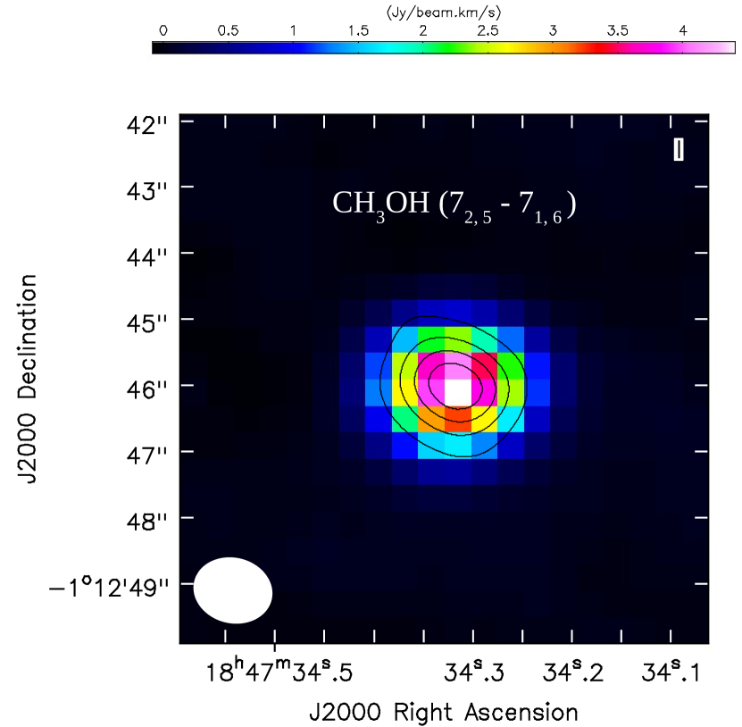
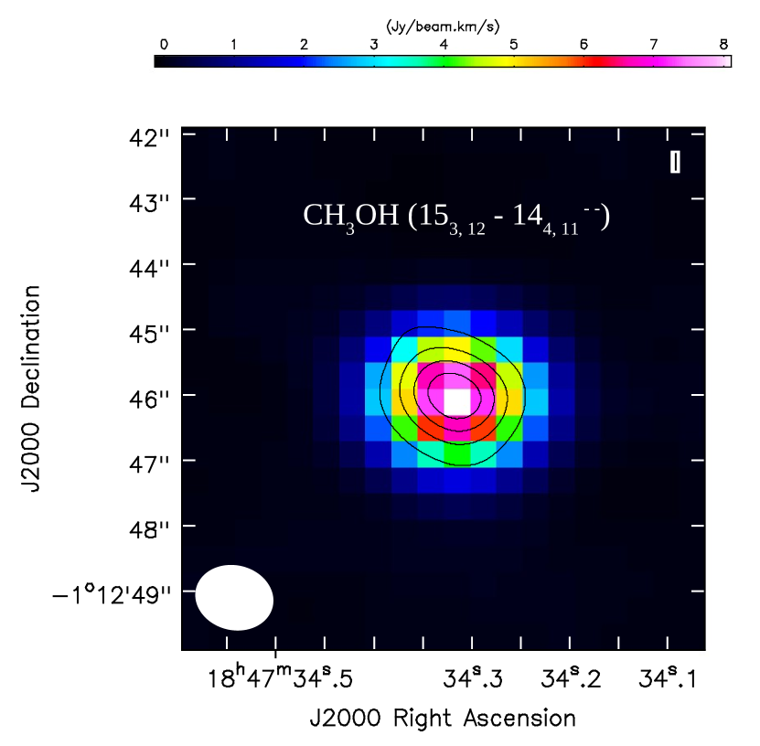
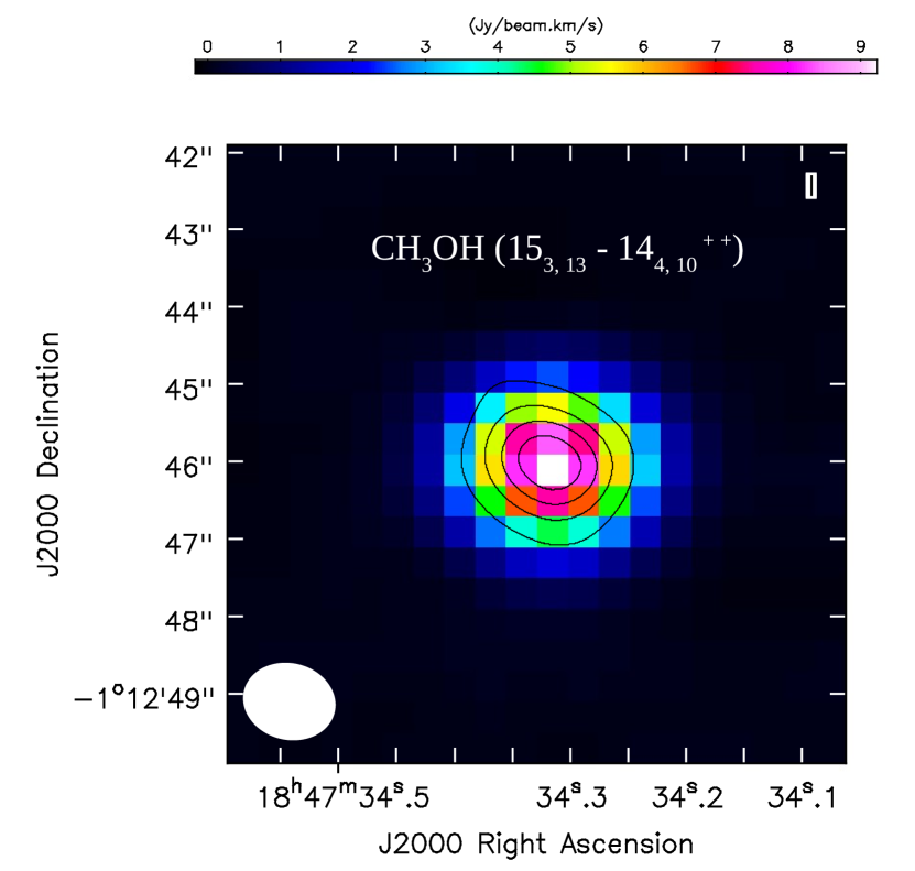
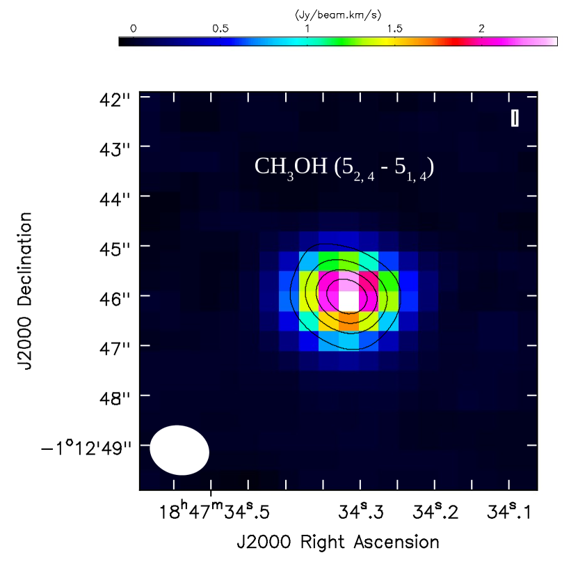
Figure 18: Moment 0 maps of the integrated intensity distribution (color) of CH₃OH transitions is overlaid on the 3.1 mm continuum emission (black contours). Contour levels are at 20%, 40%, 60 %, and 80% of the peak flux of the continuum image. The synthesized beam is shown in the lower left-hand corner of each figure.

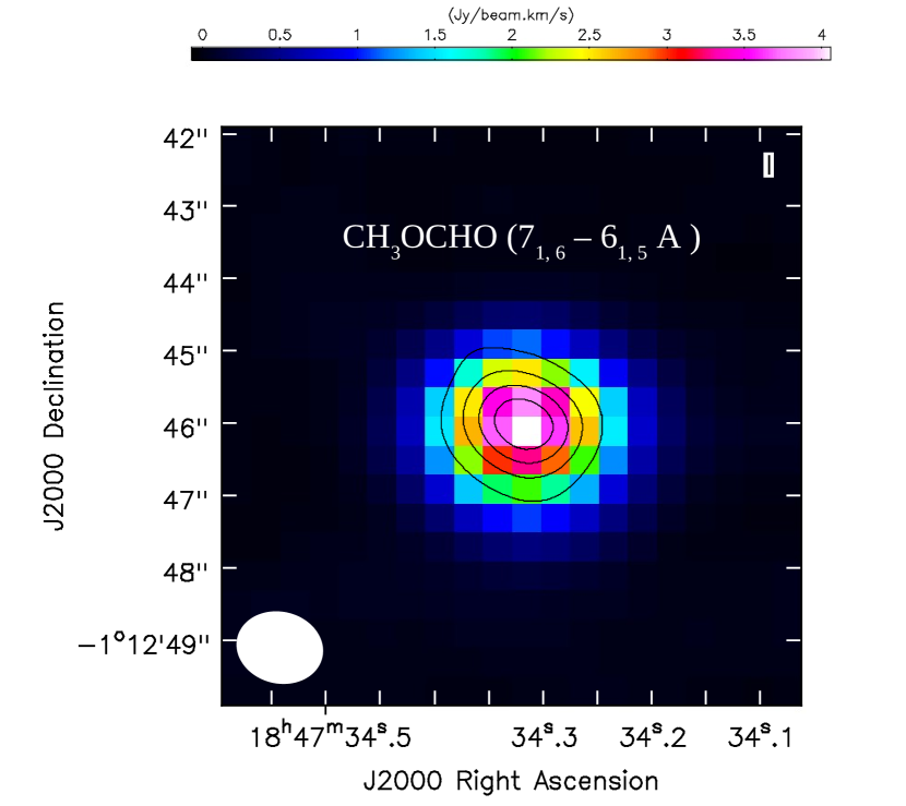
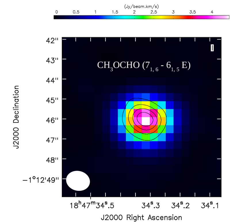
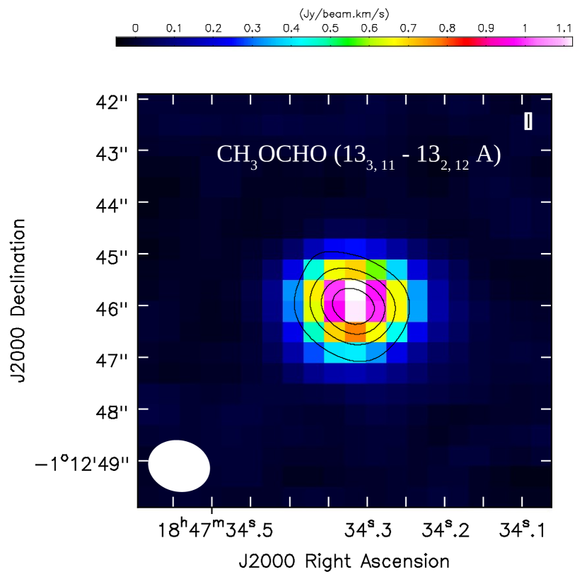
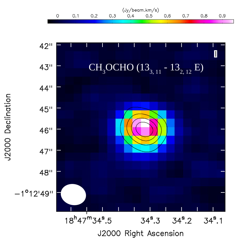
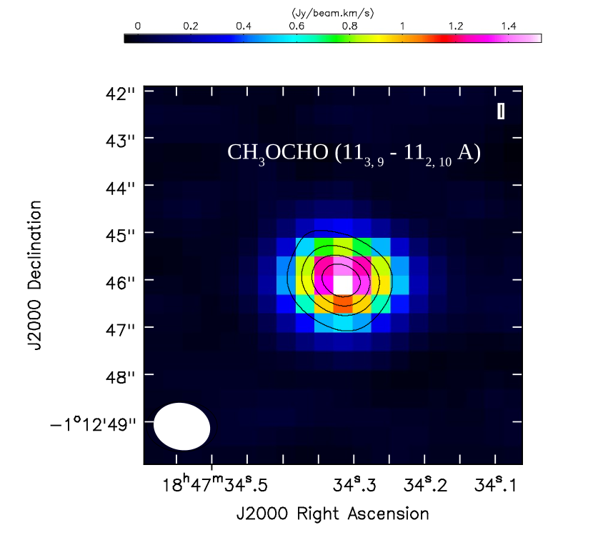
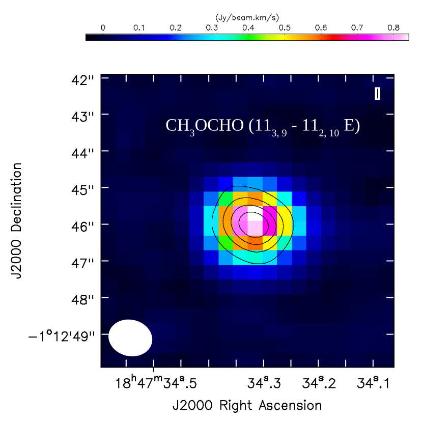
Figure 19: Moment 0 of the integrated intensity distribution (color) of CH₃OCHO transitions is overlaid on the 3.1 mm continuum emission (black contours). Contour levels are at 20%, 40%, 60 %, and 80% of the peak flux of the continuum image. The synthesized beam is shown in the lower left-hand corner of each figure.

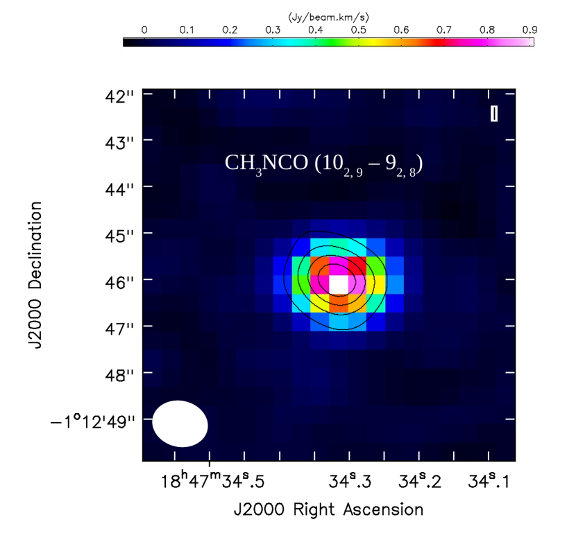
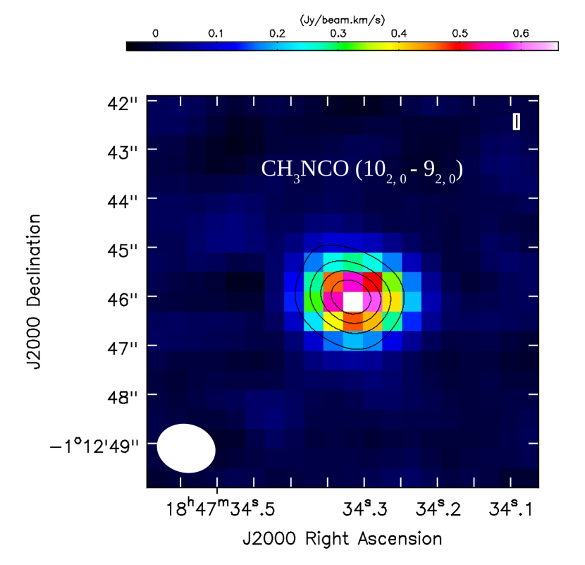
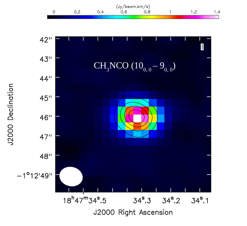
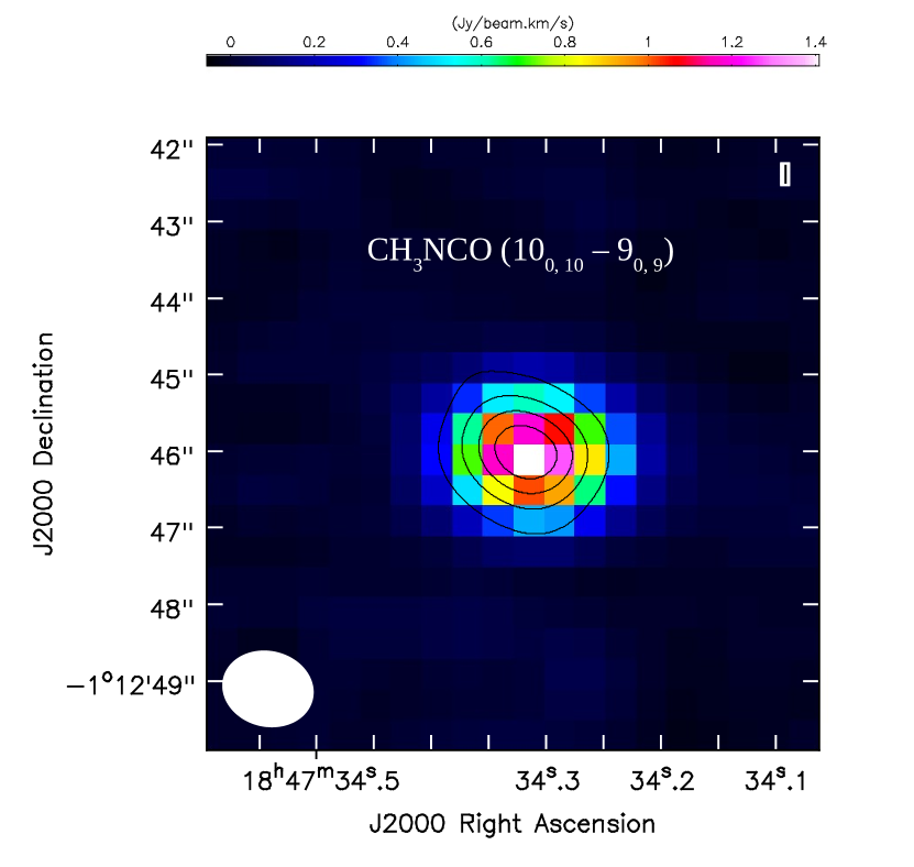
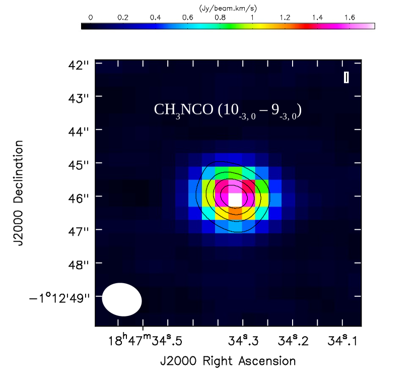
Figure 20: Moment 0 of the integrated intensity distribution (color) of CH₃NCO transitions is overlaid on the 3.1 mm continuum emission (black contours). Contour levels are at 20%, 40%, 60 %, and 80% of the peak flux of the continuum image. The synthesized beam is shown in the lower left-hand corner of each figure.

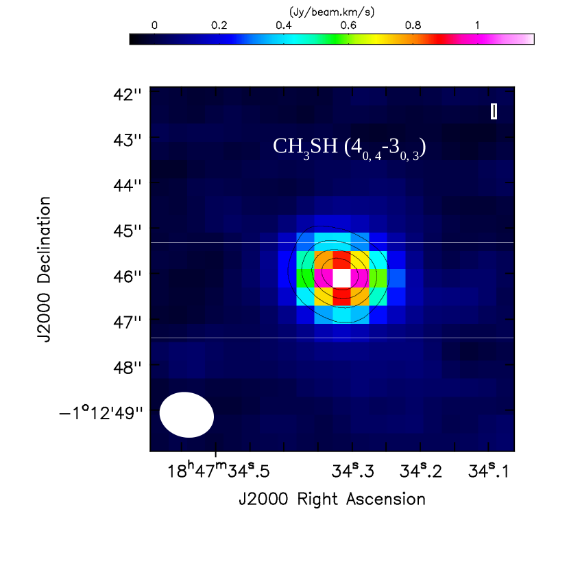
Figure 21: Moment 0 of the integrated intensity distribution (color) of CH₃SH transitions is overlaid on the 3.1 mm continuum emission (black contours). Contour levels are at 20%, 40%, 60 %, and 80% of the peak flux of the continuum image. The synthesized beam is shown in the lower left-hand corner of each figure. Multiple transitions (101.13915/101.13965 GHz) appear in CH₃SH 4_0,4-3_0,3 moment maps. Similarly multiple transitions (101.16715/101.16830 GHz) appear in CH₃SH 4_2,2-3_2,1 moment maps.

We also have identified the presence of two abundant COMs methanol and methyl formate in this source. Methanol is one of the most abundant COMs in star-forming regions. Here, we have identified seven transitions of CH₃OH with different upper state energy in the ALMA band 3 regions. We have also identified CH₃OCHO transitions with a wide range of upper-level energies ($17-207$ K), which are listed in Table 1. The integrated intensity maps of some unblended transitions of SO₂, H₂CO, CH₃SH, CH₃OH, CH₃OHCO, and CH₃NCO are shown in Figures 3(a-f) where continuum is overlaid on the integrated intensity map, and all other maps correspond to different frequencies are given in the Appendix (see Figures 18-21). Using local thermodynamic equilibrium modeling and comparing with the integrated intensities of observed molecular transitions, we found that various transitions of CH₃OH, CH₃NCO, and CH₃OCHO are optically thin.

For example, in LTE and optically thin condition, the expected line ratio between the 87.01608 GHz and 86.68019 GHz transitions of CH₃NCO is 1.6 while the observed intensity (brightness temperature) ratio is 1.44. This suggests that these two lines are optically thin. Similarly for 86.78078 GHz and 86.68019 GHz transitions of CH₃NCO, the observed intensity ratio between these two lines is 1.35, and the expected line ratio is 1.30. For the 101.12685 GHz and 101.46980 GHz transitions of CH₃OH, the observed intensity ratio is 2.3, which is consistent with the expected LTE line ratio of 2.2. For of CH₃OCHO, the observed line ratio between 88.68688 GHz and 88.85160 GHz transition is 4, which is similar to the observed integrated intensity ratio 3.7. The similarity between the expected and observed line ratios of these transitions suggest that they are optically thin.

3.3 Rotation diagram analysis: estimation of gas temperature

We have detected multiple transitions of CH₃OH, CH₃OCHO, CH₃SH, and CH₃NCO, with different $\rm{E_{u}}$. Thus, we employed the rotation diagram analysis to obtain the rotational temperatures. We performed the rotation diagram analysis by assuming the observed transitions to be optically thin and are in Local Thermodynamic Equilibrium (LTE). For optically thin lines, column density can be expressed as (Goldsmith & Langer., 1999),

$$\frac{N_{u}^{thin}}{g_{u}}=\frac{3k_{B}\int{T_{mb}dV}}{8\pi^{3}\nu S\mu^{2}},$$ (5)

where g_u is the degeneracy of the upper state, $\rm{k_{B}}$ is the Boltzmann constant, $\rm{\int T_{mb}dV}$ is the integrated intensity, $\nu$ is the rest frequency, $\mu$ is the electric dipole moment, and S is the transition line strength. Under LTE conditions, the total column density can be written as,

$$\frac{N_{u}^{thin}}{g_{u}}=\frac{N_{total}}{Q(T_{rot})}\exp^{-E_{u}/k_{B}T_{rot}},$$ (6)

where $T_{rot}$ is the rotational temperature, E_u is the upper state energy, $\rm{Q(T_{rot})}$ is the partition function at rotational temperature. The equation 6 can be rearranged as,

$$log\Bigg{(}\frac{N_{u}^{thin}}{g_{u}}\Bigg{)}=-\Bigg{(}\frac{log\ e}{T_{rot}}\Bigg{)}\Bigg{(}\frac{E_{u}}{k_{B}}\Bigg{)}+log\Bigg{(}\frac{N_{total}}{Q(T_{rot})}\Bigg{)}.$$ (7)

Equation 7 shows that there is a linear relationship between E_u and $\rm{log(N_{u}/g_{u})}$. Two parameters, column density and rotational temperature can be obtained by fitting a straight line to the values of $\rm{log(N_{u}/g_{u})}$ plotted as a function of E_u, where $\rm{N_{u}/g_{u}}$ is obtained from the observations through equation 5.

Rotational diagrams of methyl isocyanate, methanol, methanethiol, and methyl formate are presented in Figure 4. For CH₃OCHO, we have several transitions, but we do not see two components. Hence we fit all the data points with a line, which are not aligned. Though we did not find a very good fitting, the obtained rotational temperature of methyl formate $\sim 162$ K is consistent with the previously measured value in this source for the same molecule (Beltrán et al., 2005; Rivilla et al., 2017). We have obtained a rotational temperature of 76 K for CH₃SH and 48 K for CH₃NCO. The rotational diagram analysis suggests two temperature components of methanol, one is a cold component, and another is a hot component. Cold component (solid black line, see Figure 4b) temperature is obtained 33 K. In contrast, hot component (solid blue line, see Figure 4b) temperature is 181 K. Rotational diagram of CH₃OH suggests that the transitions associated with the higher $\rm{E_{u}}$ transitions (86.61557 GHz, 86.90291 GHz, 88.59478 GHz, 88.93997 GHz; hot component) are mainly arising from the hot gas surrounding the G31. In contrast, the emissions associated with the lower $E_{u}$ (101.12685 GHz, 101.29341 GHz,101.46980 GHz; cold component) transitions are from the cold region of the HMC. However, due to our observation’s lower angular and spatial resolution, we marginally resolved these transitions. Therefore, it is not possible to provide a clear insight into the spatial distribution of methanol in this source.

The error bars (vertical red bars) in Figure 4 are the absolute uncertainty in a log of (N_u/g_u), and this arises from the error of the observed integrated intensity that we measured using a single Gaussian fitting to the observed profile of each transition. The integrated intensities with their uncertainties of all observed transitions are provided in Table 1. Our estimated rotational temperatures for methyl formate and the hot component of methanol are similar to the typical hot core temperature. On the other hand, methyl isocyanate and the cold component of methanol have lower rotational temperatures (33-48 K). However, due to poor angular resolution, we could not provide further details about these two temperature components’ spatial distribution.

To obtain the molecular column density of the observed chemical species, we used LTE modeling with CASSIS. For this modeling, we used the estimated rotational temperature discussed above. We calculated beam average column density (N_b), where the effect of beam dilution was not taken into consideration. For the model, we used five parameters; (i) column density, (ii) excitation temperature (T_ex), (iii) line width ($\Delta$V), (iv) velocity (V_LSR), and (v) source size ($\theta_{s}$). To obtain the best fit with the observation, only column density was varied by keeping all other parameters (Tex, source size, FWHM, and hydrogen column density) fixed and we choose the best fitted-results when LTE model spectra are the same as the observed spectra. For LTE fitting, we used the source sizes for molecular emission similar to the deconvolved size as we obtained from 2D Gaussian fitting. Line width (FWHM) for molecular transitions are estimated from the Gaussian fitting of spectral profiles, and excitation temperature (Tex) is assumed to be $\sim$ 150 K, a typical hot core temperature. Fixed parameters are noted in Table 3. We did not have a rotation diagram for all the species (e.g., SO₂, H₂CO) presented here. Thus, we followed the LTE model to derive the column density of all the species. We have also compared the column densities of CH₃OH, CH₃SH, CH₃NCO, and CH₃OCHO between rotation diagram analysis and LTE model (see Table 4 and Section 3.6). Observed column densities and fractional abundances of all the species are presented in Table 4. Abundances of all species are noted w.r.to H₂.

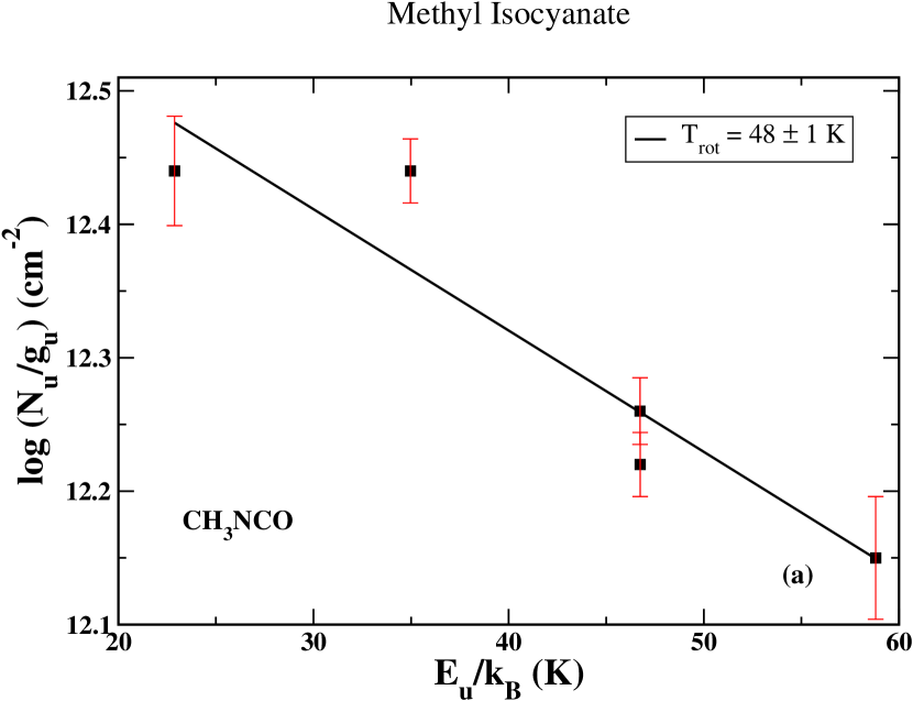
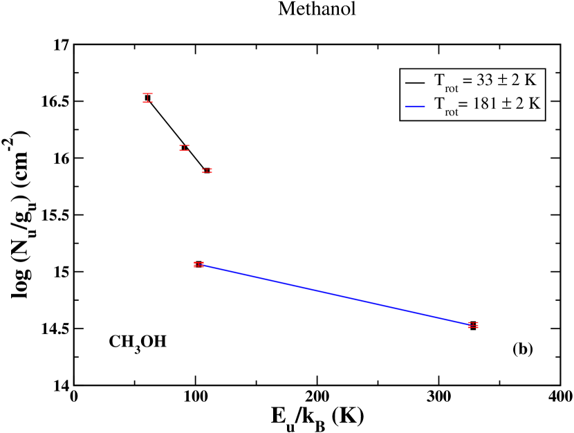
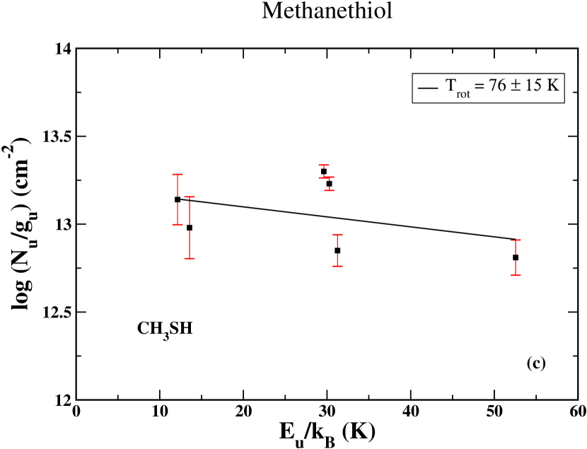
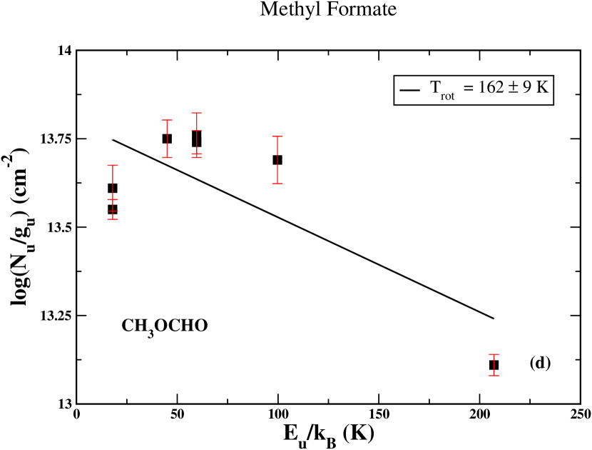
Figure 4: Rotational diagram of (a) CH₃NCO, (b) CH₃OH, (c) CH₃SH, and (d) CH₃OCHO. Black filled square shows the data points, and the solid black and blue lines represent the fitted curve.

Table 1: Summary of the line parameters of observed molecules towards G31.41+0.31.

Species	(${\rm J^{{}^{\prime}}_{K_{a}^{{}^{\prime}}K_{c}^{{}^{\prime}}}}$-${\rm J^{{}^{\prime\prime}}_{K_{a}^{{}^{\prime\prime}}K_{c}^{{}^{\prime\prime}}}}$)	Frequency (GHz)	Eu/kB (K)	FWHM (km s-1)	Peak Intensity, Iν (K)	VLSR (km s-1)	S$\mu^{2}$(Debye2)	${\int{T_{mb}}dv\ (K.km/s)}$
SO2	$\rm{8_{3,5}-9_{2,8}}$	86.63908	55.20	8.46	14.63	97.27	3.01	131.9$\pm$3.6
H2CO	$\rm{6_{1,5}-6_{1,6}}$	101.33299	87.57	10.20	75.90	97.26	5.05	824.4$\pm$22.4
CH3SH	$\rm{4_{0,4}-3_{0,3}}$ (A$+$)	101.139151	12.14	8.70	6.00	97.00	6.61	55.2$\pm$17.7
	$\rm{4_{0,4}-3_{0,3}}$ (E$+$)	101.139651	13.56	6.10	5.90	95.45i	6.61	38.5$\pm$14.8
	$\rm{4_{2,3}-3_{2,2}}$ (A$-$)	101.159332	31.26	6.75	3.50	97.00	4.96	26.1$\pm$4.7
	$\rm{4_{3,2}-3_{3,1}}$ (E$-$)	101.159992	52.39	7.09	1.56	95.03ii	2.90	13.1$\pm$2.9
	$\rm{4_{3,1}-3_{3,0}}$ (A$+$)	101.160662	52.55	7.09	1.56	93.05ii	2.90	13.1$\pm$2.9
	$\rm{4_{3,2}-3_{3,1}}$ (A$-$)	101.160692	52.55	7.09	1.56	92.94ii	2.90	13.1$\pm$2.9
	$\rm{4_{2,3}-3_{2,2}}$ (E$-$)	101.167153	29.62	6.94	8.20	97.00	4.96	60.6$\pm$5.2
	$\rm{4_{2,2}-3_{2,1}}$ (E$+$)	101.168303	30.27	6.20	7.70	93.58iii	4.96	50.8$\pm$4.5
CH3OH	$\rm{7_{2,5^{-}}-6_{3,3^{-}},v_{t}=0}$	86.61557	102.70	9.06	84.55	97.02	1.35	815.3$\pm$26.8
	$\rm{7_{2,5^{+}}-6_{3,4^{+}},v_{t}=0}$	86.90291	102.72	9.13	85.16	97.00	1.35	827.8$\pm$24.9
	$\rm{15_{3,13^{+}}-14_{4,10^{+}},v_{t}=0}$	88.59478	328.26	8.98	82.26	97.10	4.20	786.4$\pm$14.6
	$\rm{15_{3,12^{+}}-14_{4,11^{-}},v_{t}=0}$	88.93997	328.28	8.55	79.78	97.16	4.20	726.5$\pm$9.9
	$\rm{5_{-2,3}-5_{1,4},E2,v_{t}=0}$	101.12685	60.73	8.37	23.87	98.88	0.01	208.4$\pm$18.8
	$\rm{7_{-2,5}-7_{1,6},E2,v_{t}=0}$	101.29341	90.91	7.72	45.71	97.38	0.05	373.2$\pm$18.0
	$\rm{8_{-2,6}-8_{1,7},E2,v_{t}=0}$	101.46980	109.49	7.25	55.31	97.98	0.09	426.9$\pm$16.5
CH3NCO	$\rm{10_{0,0}-9_{0,0}}$	86.68655	34.97	7.70	14.63	97.83	83.11	120.0$\pm$6.8
	$\rm{10_{0,10}-9_{0,9}}$	86.68019	22.88	8.28	13.50	97.90	83.06	119.1$\pm$11.5
	$\rm{10_{2,9}-9_{2,8}}$	86.78077	46.73	6.80	10.45	97.32	79.73	75.8$\pm$4.5
	$\rm{10_{2,8}-9_{2,7}}$	86.80502	46.74	5.82	11.16	97.10	79.74	69.2$\pm$3.8
	$\rm{10_{-3,0}-9_{-3,0}}$	86.86674	88.58	10.14	15.80	97.00	75.32	170.6$\pm$16.6
	$\rm{10_{2,0}-9_{2,0}}$	87.01607	58.88	6.22	8.91	97.12	79.18	59.0$\pm$6.2
	$\rm{10_{0,10}-9_{0,9}}$	86.67492	285.03	–	–	–	83.07	–
CH3OCHO	$\rm{17_{3,14}-17_{3,15}}$	86.91761	99.72	6.41	7.09	98.03	1.87	48.5$\pm$7.6
	$\rm{11_{3,9}-11_{2,10}}$ E	88.68688	44.97	5.41	12.90	97.86	2.44	74.3$\pm$9.2
	$\rm{11_{3,9}-11_{2,10}}$ A	88.72326	44.96	7.84	17.11	98.32	2.43	142.8$\pm$29.0
	$\rm{7_{1,6}-6_{1,5}}$ E	88.84318	17.96	8.07	45.87	98.18	18.04	394.3$\pm$58.9
	$\rm{7_{1,6}-6_{1,5}}$ A	88.85160	17.94	6.64	49.17	97.50	18.04	348.0$\pm$22.4
	$\rm{8_{1,8}-7_{1,7}}$ E	88.86241	207.10	5.83	23.49	97.64	20.89	145.9$\pm$10.1
	$\rm{13_{3,11}-13_{2,12}}$ E	101.37050	59.64	5.16	15.90	97.93	2.61	87.4$\pm$6.7
	$\rm{13_{3,11}-13_{2,12}}$ A	101.41474	59.63	5.93	14.56	97.81	2.60	92.0$\pm$13.5
SiO	(2-1)	86.84696	6.25	–	–	94.1	2.82	–

NOTES: ¹ Spectral profile 1, ² Spectral profile 2, ³ Spectral profile 3, ⁱ velocity with respect to 101.13915 GHz transition, ⁱⁱ velocity w.r.t 101.15933 GHz transition, ⁱⁱⁱ velocity w.r.t 101.16715 GHz transition.

Table 2: Observed molecular transitions in absorption.

Species	(${\rm J^{{}^{\prime}}_{K_{a}^{{}^{\prime}}K_{c}^{{}^{\prime}}}}$-${\rm J^{{}^{\prime\prime}}_{K_{a}^{{}^{\prime\prime}}K_{c}^{{}^{\prime\prime}}}}$)	Frequency in GHz	Eu (K)
H13CO+	1-0	86.75430	4.16
HCN	1-0(F=1-1)	88.63041	4.25
HCN	1-0(F=2-1)	88.63184	4.25
HCN	1-0(F=0-1)	88.63393	4.25

Table 3: Input parameters of LTE model

Species	Source size (′′)	FWHM (km/s)
SO2	0.7	8.4
H2CO	1.3	10.2
CH3SH	0.8	5.5
CH3OH	1.3	8.5
CH3NCO	0.8	6.5
CH3OCHO	1.35	6.0

H₂ column density = $\rm{1.53\times 10^{25}\ cm^{-2}}$
T_ex =150 K

Table 4: Comparison of observed molecular column density, fractional abundances, and molecular ratios between G31 and other sources.

Species	G31.41+0.31,		Sgr B2 (N)	Orion KL	G10.47+0.03	Chemical Model
	Column density		Column density	Column density	Column density	Column density
	[Abundance]		[Abundance]	[Abundance]	[Abundance]	[Abundance]
	LTE            Rotation Diagram
CH3OH	1.84(19)[1.2(-6)]∗	2.94(19)[1.92(-6)]	4.00(19)[1.14(-5)]a	3.24(18)[1.62(-6]f	9.0(18)[1.8(-6)]m	7.56(19)[2.10(-5)]n
CH3OCHO	6.50(18)[4.25(-7)]	4.30(18)[2.81(-7)]	1.20(18)[3.33(-7)]b	1.04(17)[5.2(-8)]g	7.0(17)[1.4(-7)]m	3.31(17)[9.20(-8)]n
CH3NCO	7.22(17)[4.72(-8)]∗	1.58(16)[1.04(-9)]	2.20(17)[6.11(-8)]c	7.0(15)[3.5(-9)]h	1.2(17)[8.88(-9)]o	4.68(16)[1.30(-8)]b
CH3SH	4.13(17)[2.70(-8)]	2.85(16)[1.86(-9)]	3.40(17)[9.44(-8)]a	2.0(15)[1.0(-9)]i	–	1.33(16)[3.70(-9)]a
SO2	2.88(18)[1.88(-7)]		8.28(16)[2.30(-8)]d	1.0(17)[5.0(-8)]j	3.0(17)[6.0(-8)]m
H2CO	2.90(18)[1.90(-7)]		1.82(17)[5.06(-8)]e	1.5(17)[7.5(-8)]k	3.0(18)[6.0(-7)]m
SiO	1.46(15)[9.54(-11)]∗∗		4.32(15)[1.20(-9)]d	5.4(14)[2.7(-10)]l	–
CH3SH/CH3OH	0.0225	0.0010	0.0082	0.0006		0.0002
CH3OCHO/CH3OH	0.3541	0.1463	0.0292	0.0321	0.0778	0.0044
CH3NCO/CH3OH	0.0393	0.0005	0.0054	0.0022	0.0049	0.0006

^aMüller et al. (2016), ^bBelloche et al. (2016), ^cBelloche et al. (2017), ^dHiguchi et al. (2015), ^eBelloche et al. (2013), ^fFavre et al. (2015), ^gFavre et al. (2011), ^hCernicharo et al. (2016), ⁱKolesniková et al. (2014), ^jTercero et al. (2018), ^kEsplugues et al. (2013), ^lSchilke et al. (2001), ^mRolffs et al. (2011),ⁿGarrod et al. (2013), ^oGorai et al. (2020)

Orion KL ($\rm{N_{H_{2}}}$)= $\rm{2.0\times 10^{24}}$cm^-2, Sgr B2(N) ($\rm{N_{H_{2}}}$)= $\rm{3.6\times 10^{24}}$cm^-2, G10.47+0.03 ($\rm{N_{H_{2}}}$)= $\rm{5.0\times 10^{24}}$cm^-2, G31.41+0.31 ($\rm{N_{H_{2}}}$)= $\rm{1.53\times 10^{25}}$cm^-2

^∗ For hot component of methanol, column density is derived using higher value of excitation temperature T = 300 K. Using LTE, we have found opacities $\geqslant$1 for a few transitions of CH₃OH (86.68655 GHz, 86.68019 GHz, 86.78077 GHz, and 86.80502 GHz) and CH₃NCO (86.68019 GHz and 86.68655 GHz). Thus, the column density estimated for CH₃OH and CH₃NCO by using LTE should be considered as lower limit.

^∗∗ SiO column density and fractional abundance calculated in the outflowing gas measured at V_LSR =94.1 km s^-1 by averaging over the box (7^′′$\times$${7^{\prime\prime}}$) centered at ($\alpha$(J2000), $\delta$ (J2000)) = [18^h47^m34.121^s, -1^o12^′48.975^′′].

3.4 Radiative transfer modeling

Absorption studies are best-suited to trace the physical conditions (e.g., density, kinetic temperature) of the ISM because it is not induced by beam dilution as long as the absorbing layer is larger than the continuum source. Here, we used non-LTE modeling to derive excitation conditions and physical properties from these absorption features. For the non-LTE modeling, we use RADEX program (Van der Tak et al., 2007). The collisional rates were taken from LAMDA database and the spectroscopic constants were taken from JPL/CDMS catalog. In RADEX, we used the continuum background temperature (T_c) of 36 K, which corresponds to the peak brightness temperature of the 3.2 mm continuum by considering the beam dilution. For this modeling, we have used colum density $\rm{3.55\times 10^{15}\ cm^{-2}}$, $\rm{8.92\times 10^{15}\ cm^{-2}}$, and $\rm{1.18\times 10^{15}\times cm^{-2}}$ for H¹³CO⁺, HCN, and SiO respectively. Figures 5(a)-(c) shows the variation of radiation temperature of HCN (1-0), $\rm{H^{13}CO^{+}}$ (1-0), and SiO (2-1) respectively for a wide range of parameter space. Our parameter space consists of the number density of hydrogen (varies in between $\rm{10^{3}-10^{7}\ cm^{-3})}$ and kinetic temperature (varies in between 1-100 K). Figures 5(a)-(c) shows the parameter space for the absorption features of HCN, $\rm{H^{13}CO^{+}}$, and SiO respectively. We have estimated the critical density of HCN (1-0), $\rm{H^{13}CO^{+}}$ (1-0), and SiO (2-1), which are 1.51$\times$10⁶ cm^-3, 1.83$\times$10⁵ cm^-3, and 2.26$\times$10⁵ cm^-3 respectively. We have shown that for hydrogen density $\geq$ 1.0$\times$10⁵ cm^-3, all these transitions are showing absorption features. If H₂ density is below the critical density, level populations are mostly governed by collisional excitation and de-excitation rather than Boltzmann distribution. . Thus these molecules might show emission even at T$\leq$T_c. The observed spectral profile of SiO is in line with this results. We found SiO emission at all positions except the source’s central region (where density is high, which is probably greater than critical density).

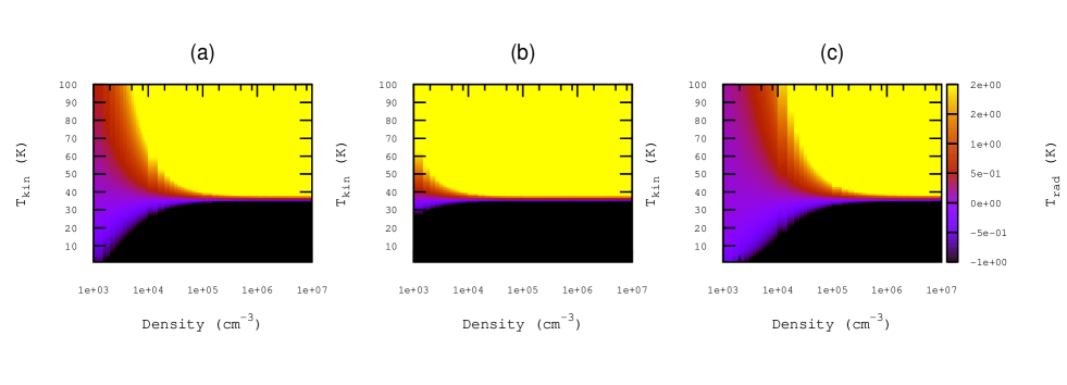
Figure 5: Variation of the radiation temperature of (a) HCN(1-0), (b) H¹³CO⁺ (1-0), and (c) SiO (2-1) respectively for a wide range of parameter space. The vertical axis is the kinetic temperature, labeled as $\rm{T_{kin}}$ (K). The units of the radiation temperature (T_rad) used in the color bar is in Kelvin.

3.5 Physical properties of the source

In this source, we obtained a temperature range 33 to 180 K. Hydrogen column density of this source is estimated $\sim{\rm 1.53\times 10^{25}}$ cm^-2. Various observed molecular emissions are discussed below.

3.5.1 Infalling envelope

Infall nature was observed in G31 earlier by various authors (Girart et al., 2009; Mayen-Gijon et al., 2014; Beltrán et al., 2018, e.g.,). Girart et al. (2009) observed an inverse P-Cygni profile in G31 with low energy lines of C³⁴S (7-6). Recently, Beltrán et al. (2018) identified red-shifted absorption of H₂CO and CH₃CN and its isotopologues towards the dust continuum of the main core with different upper state energy. Mayen-Gijon et al. (2014) observed various inversion transitions (2,2), (3,3), (4,4), (5,5) and (6,6) of ammonia by using Very Large Array (VLA) observations to understand the infall motion in G31. To explain the infall motion in G31, they used a different approach called the central blue spot which can be easily identified in the first-order moment maps. The central blue spot consists of blue-shifted emission in the first-order moment towards the zeroth-order moment map’s peak position. They found the central blue spot infall signature in all observed transitions of ammonia. In this work, we have detected one transition of H¹³CO⁺ (1-0) at frequency $86.75430$ GHz, which shows both absorption and emission nature (see Figure 2a). This is an inverse P-Cygni profile. The infall velocity can be estimated as the difference between systematic velocity and the velocity at the observed inverse P-Cygni profile’s absorption feature. The infall velocity of the source is obtained to be 4.5 km s^-1. This suggests that matter is infalling from the envelope towards the source’s central region, which is consistent with the earlier observations (Girart et al., 2009; Beltrán et al., 2018).

3.5.2 Molecular outflow

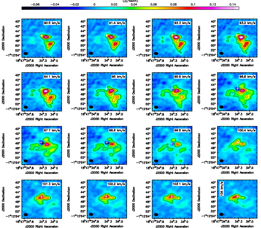
Figure 6: Channel maps of SiO (2-1) emission. Ellipse at the below left corner of the image shows the beam size $\rm{1.52^{\prime\prime}\times 1.09^{\prime\prime}}$ with PA=88.98^o. White plus sign indicates the position of the continuum.

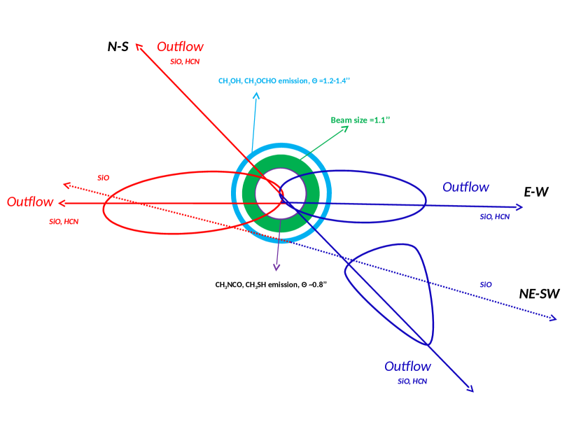
Figure 10: Schematic diagram (not up to scale) of kinematics and molecular distribution in G31.41+0.31 based on present observational results (see details in the Section 3.6.6).

Many authors previously studied molecular outflows associated with G31 (e.g., Cesaroni et al., 2011; Olmi et al., 1996; Beltrán et al., 2018). SiO and $\rm{{}^{13}CO}$ revealed the presence of two molecular outflows: One in the East-West (E-W) direction and another one in the North-South (N-S) direction. SiO is an excellent tracer of shock and molecular outflow associated with the star-forming regions (e.g., Zapata et al., 2009; Leurini et al., 2014). Beltrán et al. (2018) showed average red-shifted and blue-shifted wings of SiO emission, which reveals three outflow directions associated with this source: E-W, N-S, and NE-SW. . Among these three outflow directions, N-S and E-W components are clearly present in our observation. However, NE-SW component is not very evident (see original Figure 7 and illustrated in Figure 10). Channel maps of SiO emission is shown in Figure 6. The blue-shifted and red-shifted integrated emission of SiO along with the continuum, is depicted in Figure 7. The presence of HCN is widespread in diverse interstellar environments ranging from dark cloud to star-forming region and circumstellar envelope of a carbon-rich star (e.g., Snyder & Buhl., 1971; Ziurys & Turner., 1986). HCN also traces molecular outflow in G31. The observed spectrum profile of HCN (see Figure 2b) is symmetric with respect to the systematic velocity of the source. However, the intensity of emission wings associated with the absorption profile is asymmetric. This may be due to the asymmetry in molecular distributions. Figure 8 shows the red-shifted and blue-shifted integrated emissions of HCN overlaid on the continuum.

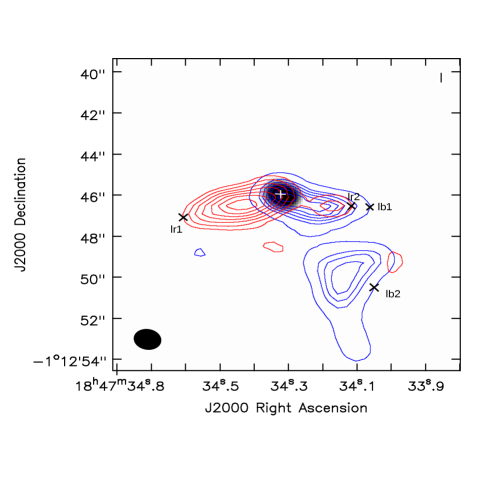
Figure 7: Gray scale levels for the continuum at 94 GHz. Blue-shifted emission of SiO integrated over 77-93 km s^-1 where contour levels are at the 20, 30, 40, 50 ,60, 70, 80 $\%$ of the peak intensity. Red-shifted emission of SiO is integrated over 100-123 km s^-1. Ellipse at the below left corner of the image shows the synthesized beam ($\rm{1.19^{\prime\prime}\times 0.98^{\prime\prime}}$). Plus sign indicates the position of the continuum. Two cross sign at the outer contour of red lobes indicates lr1 and lr2 distance another two cross sign on the red lobes indicated lb1 and lb2 distance.

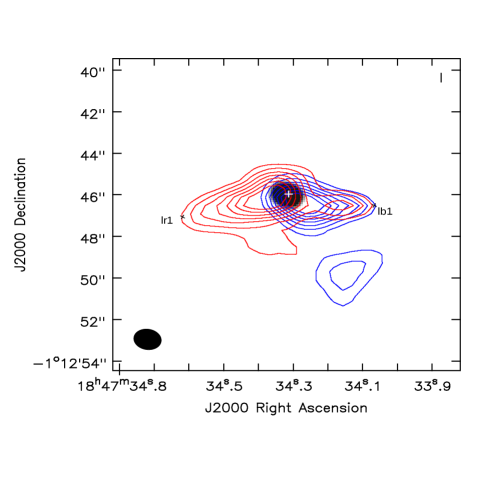
Figure 8: Gray scale levels are used for the continuum at 94 GHz. Blue-shifted emission of HCN integrated over 77-90 km s^-1 contours levels are at the 20, 30, 40, 50 ,60, 70, and 80$\%$ of the peak intensity. Red-shifted emission of HCN integrated over 105-115.7 km s^-1. Ellipse at the below left corner of the image shows the synthesized beam ($\rm{1.19^{\prime\prime}\times 0.98^{\prime\prime}}$) with PA=76.83^o

Table 5: Physical parameters of the outflow

Parameters	SiO	HCN
Distance from continuum position to outer contour (pc)
Red lobe (lr1)	0.117 (0.055)	0.118 (0.055)
Red lobe (lr2)	0.087 (0.041)	–
Blue lobe1 (lb1)	0.108 (0.051)	0.09 (0.042)
Blue lobe2 (lb2)	0.135 (0.063)	–
Typical outflow velocity: Voutflow (km s-1)
Red lobe	33.0	40.0
Blue lobe	23.0	30.0
Dynamical time: tdyn (yr)
Blue lobe	$\rm{4.59\times 10^{3}}$ ($\rm{1.62\times 10^{3}}$)	$\rm{2.87\times 10^{3}}$ ($\rm{1.35\times 10^{3}}$)
	$\rm{5.74\times 10^{3}}$ ($\rm{1.21\times 10^{3}}$)	–
Red lobe	$\rm{3.47\times 10^{3}}$ ($\rm{2.16\times 10^{3}}$)	$\rm{2.90\times 10^{3}}$ ($\rm{1.36\times 10^{3}}$)
	$\rm{2.58\times 10^{3}}$ ($\rm{2.70\times 10^{3}}$)	–
Average	$\rm{4.10\times 10^{3}}$ ($\rm{1.92\times 10^{3}}$)	$\rm{2.88\times 10^{3}}$ ($\rm{1.36\times 10^{3}}$)
Outflow mass ($\rm{M_{\odot}}$)
Blue lobe	27 (6)	12 (2.6)
Red lobe	24 (5)	55 (12)
Total	51 (11)	67 (14.6)
Momentum ($\rm{M_{\odot}}$ km s-1)
Blue lobe	619 (136)	352 (77)
Red lobe	790 (173)	2213 (485)
Total	1409 (309)	2565 (562)
Kinetic energy ($\rm{L_{\odot}}$ yr)
Blue lobe	$\rm{7.1\times 10^{3}}$ ($\rm{1.6\times 10^{3}}$)	$\rm{5.3\times 10^{3}}$ ($\rm{1.2\times 10^{3}}$)
Red lobe	$\rm{1.3\times 10^{4}}$ ($\rm{8.8\times 10^{3}}$)	$\rm{4.4\times 10^{4}}$ ($\rm{9.7\times 10^{3}}$)
Total	$\rm{2.0\times 10^{4}}$ ($\rm{1.0\times 10^{4}}$)	$\rm{4.9\times 10^{4}}$ ($\rm{1.1\times 10^{4}}$)
Mass loss ($\rm{M_{\odot}}$ yr-1)
Blue lobe	$\rm{5.2\times 10^{-3}}$ ($\rm{4.1\times 10^{-3}}$)	$\rm{4.1\times 10^{-3}}$ ($\rm{1.9\times 10^{-3}}$)
Red lobe	$\rm{7.9\times 10^{-3}}$ ($\rm{2.1\times 10^{-3}}$)	$\rm{1.9\times 10^{-2}}$ ($\rm{8.9\times 10^{-3}}$)
Total	$\rm{1.3\times 10^{-2}}$ ($\rm{6.2\times 10^{-3}}$)	$\rm{2.3\times 10^{-2}}$ ($\rm{10.8\times 10^{-3}}$)
Momentum loss ($\rm{M_{\odot}}$ km s-1 yr-1)
Blue lobe	0.12 (0.09)	0.12 (0.06)
Red lobe	0.26 (0.07)	0.76 (0.35)
Total	0.38 (0.16)	0.88 (0.41)
Energy loss ($\rm{L_{\odot}}$)
Blue lobe	1.38 (1.10)	1.84 (0.85)
Red lobe	4.31 (3.63)	15.26 (7.14)
Total	5.69 (4.73)	17.10 (7.99)

Note: To estimate the SiO outflow physical parameters, we considered average value of red lobe (r_r=$\frac{lr1+lr2}{2}$) and blue lobe (r_b=$\frac{lb1+lb2}{2}$) and their corresponding average time scale of blue lobe and red lobe. We have calculated the lobe distance in arcsec and then convert into parsec by considering source distance 7.9 kpc. In parenthesis, we have noted the outflows parameters by considering the new distance 3.7 kpc of G31.

To obtain the outflow parameters, we estimated the outflow velocity as the maximum velocity of outflow emission with respect to the systematic LSR velocity ($97$ km s^-1). For the blue lobe and red lobe of SiO outflow, velocities are found to be $23$ km s^-1 and $33$ km s^-1. We estimated the dynamical timescale of outflow by using t_dyn =$\frac{l(b,r)}{V_{max}(b,r)}$. For this, we calculate two different lengths (lb1, lb2) of the blue lobe and two lengths (lr1, lr2) for red lobes (see Figure 7-8). We obtained the average dynamical time scale of outflow $\sim$ $\rm{4\times 10^{3}}$ years by considering the maximum velocity of SiO of the blue lobe and red lobe. The dynamical time scale of HCN outflow is obtained to be $\sim$ $\rm{3\times 10^{3}}$ years. These values are in good agreement with the dynamical time scale of outflow of ¹²CO and SiO, as previously reported in G31 by Cesaroni et al. (2011) and Beltrán et al. (2018). For all individual positions, the different dynamical time scales for both blue and red lobe are presented in Table 5. For HCN, we calculate the outflow parameters for one blue lobe (lb1) and one red lobe (lr1). To estimate the other outflow parameters such as mass, momentum, energy, mass loss, momentum loss, and energy loss per year, we used the formula mentioned in Cabrit & Bertout. (1990). To estimate the outflow parameters, we assumed same abundance ($\rm{1.0\times 10^{-8}}$) and excitation temperature ($20$ K) of SiO (Codella et al., 2013) and HCN. All the outflow parameters are summarized in Table 5. All these outflow parameters are in good agreement with the observed values of Araya et al. (2008).

In Figure 6, we have shown the channel maps of SiO emission associated with the HMC. This figure depicts that blue-shifted channels are distributed in the southwest region and red-shifted channels toward the south-east and north-east regions. Bipolar lobe morphology observed from 93.2 km s^-1 and 103.1 km s^-1 channels suggest wide-angle bipolar outflow. Integrated emission of SiO and HCN transition (Figures 7 and 8) shows that there is a clear outflow direction along the East-West direction. In the integrated emission, the red lobe of outflow is slightly tilted to the south-east. This may occur due to another outflow direction along the southwest-northeast direction. There is also an outflow in the N-S direction. Outflow of HCN along the N-S direction is wider (see Figure 8) as compared to the SiO outflow (see Figure 7). This may be attributed to the excitation conditions and chemical origin of HCN. The estimated outflow is massive, 50 M_⊙ for SiO and 67 M_⊙ for HCN and the outflow is characterized as young (3-4$\rm{\times 10^{3}}$ years). However, by considering the new distance measurement of $\sim 3.7$ kpc of this source, we obtained the dynamical time scale of outflow around 1-2$\rm{\times 10^{3}}$ years. The estimated outflow mass is $\sim$11 M_⊙ for SiO and $\sim$14.6 M_⊙ for HCN.

3.6 Molecular distributions and abundances

In this section, we present the molecular abundance of all the observed species. We compare the abundance of all detected species between G31 and other sources, which is presented in Table 4. All the molecular abundances are reported w.r.t. H₂. Figure 10 in the Appendix shows the schematic diagram of kinematics and molecular distributions of G31 based on present observation. There are three outflow directions one is along the E-W direction, one is along the N-S direction, and another is along the NE-SW direction (only for SiO). Outflow components are traced by HCN and SiO emissions. Here, we have obtained different molecular distributions of COMs. The emitting regions of different transitions of COMs are different. We have separated those into three regions such as the emitting region is smaller than the beam size ($\rm{\theta\sim 0.8^{{}^{\prime\prime}}}$, see the purple circle in the Figure 10), comparable to the beam size ($\rm{\theta\sim 1.1^{{}^{\prime\prime}}}$, see green circle outer edge in the Figure 10), and greater than the beam size ($\rm{\theta\sim 1.4^{{}^{\prime\prime}}}$, see cyano circle in the Figure 10). Emitting region of all observed species are provided in Table 6 (see in Appendix). The uncertainties of emitting regions listed in Table 6 are the lower limit of true values as estimated emitting regions might be affected by several issues such as poor angular resolution, image noise, and non-Gaussian shape of the source. Emitting regions of CH₃OH and CH₃OCHO are comparable or slightly greater as compared to the beam size. Molecular distributions show that CH₃NCO and CH₃SH have a slightly lower-emitting region as compared to beam size (marginally resolved). The data presented in this paper suggests possibly different emitting regions for different COMs, but these are not conclusive because of comparable beam and source size. High sensitivity data with high angular and spatial resolution is required to understand the spatial distributions of these molecules.

3.6.1 Sulfur dioxide, SO₂

SO₂ is a good tracer of dense and hot gas of typical hot core (e.g., Charnley et al., 1997; Leurini et al., 2007). In this source, we detected a strong transition ($\rm{8_{3,5}-9_{2,8}}$) of SO₂. Using LTE model, we estimated the column density and the fractional abundance of SO₂, which are $\sim 2.88\rm{\times 10^{18}}$ cm^-2 and 1.88$\rm{\times 10^{-7}}$. The observed abundance of SO₂ in G31 is one order of magnitude higher as compared to Srg B2, Orion KL and G10.47+0.03.

3.6.2 Formaldehyde, H₂CO

The presence of H₂CO with its ortho, para, and isotopic form within the frequency range of $218-364$ GHz was previously reported by Isokoski, Bottinelli & van Dishoeck. (2013). Red-shifted strong absorption of H₂CO (E_up=21 K, 68 K) had recently been observed in G31, which supports the existence of infall in the core (Beltrán et al., 2018). Previously, Di Francesco et al. (2001) reported a similar kind of inverse P-Cygni profile and found that H₂CO traces infall in IRAS 4A and they also detected the outflow from both 4A and 4B position by observing bright wing emission of H₂CO. Formaldehyde, along with its deuterated counterpart, has also been observed in outflows toward other sources (e.g., Sahu et al., 2018). The presence of H₂CS in G31 has previously been reported by Ligterink et al. (2015). Here, we also have detected one strong emission line of H₂CS at 101.478 GHz. However, the observed spectrum of H₂CS shows that there is a blending with other molecular lines (methyl formate, confirmed from LTE modeling). “H₂CO and H₂CS are ubiquitous in the ISM. These two species have similar chemical structures; just O atom of H₂CO is replaced by S atom in H₂CS.

3.6.3 Methanol, CH₃OH

Methanol is a well-known and one of the most abundant COMs in hot cores. Here, we have identified several transitions of methanol. LTE model suggests that it has a high fractional abundance $\sim 1.2\rm{\times 10^{-6}}$. We have also estimated methanol abundance following rotation diagram analysis.The obtained abundance using rotation diagram analysis is $\sim 1.2\rm{\times 10^{-6}}$, which is similar to the estimated results using the LTE model. A comparison of fractional abundance of methanol between G31 and other hot molecular core is presented in Table 4.

3.6.4 Methanethiol, CH₃SH

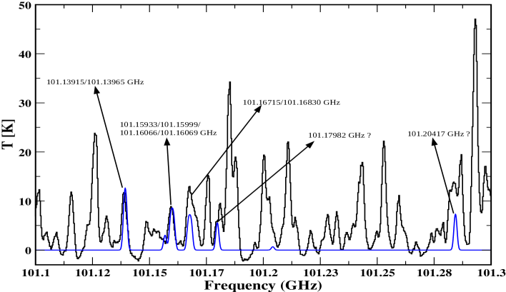
Figure 16: Black line represents observed spectra and blue line represents the (LTE) model spectra of methanethiol (CH₃SH). In addition to the observed transitions of CH₃SH listed in Table 1, we have also see signature of two other transitions (101.17982 GHz and 101.20417 GHz), which are heavily blended with other species.

Methanethiol has a similar chemical structure as methanol; just O atom of methanol is replaced by S atom of methanethiol. In Figure 16, we show the observed and model (LTE) spectra of CH₃SH. Best fitted abundance and column density of methanethiol are $\sim 2.70\rm{\times 10^{-8}}$ and $\sim 4.13\rm{\times 10^{-17}}$ respectively. We also estimated the column density and fractional abundance of this species using rotation diagram analysis, which is one order of magnitude lower as compared to LTE model fitted results. The observed emitting region of methanethiol is comparable to the beam size. The spatial distribution of its emission is as compact as the dust continuum. Since our beam size is comparable to the source size. Therefore, we have uncertainties in determining the emitting regions of this species. For detail knowledge about the distribution of this species, we need a high angular and spatial resolution data.

3.6.5 Methyl formate, CH₃OCHO

CH₃OCHO is one of the most abundant COMs, which was observed in both low-mass and high-mass star-forming regions (e.g., Brown et al., 1975; Cazaux et al., 2003). Previously, numerous transitions of CH₃OCHO were identified in G31 (Isokoski, Bottinelli & van Dishoeck., 2013; Rivilla et al., 2017; Beltrán et al., 2018). Column density, fractional abundance, and a comparison of fractional abundance of methyl formate with other hot cores are provided in Table 4. The estimated column density and fractional abundance of methyl formate are similar using both rotation diagram and LTE model fitting analysis. Emitting diameters of various transitions of CH₃OCHO are noted down in Table 6.

3.6.6 Methyl isocyanate, CH₃NCO

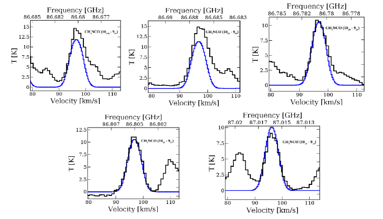
Figure 17: Black line represents observed spectra and blue line represents the (LTE) model spectra of methyl isocyanate (CH₃NCO).

In the case of CH₃NCO, we have obtained a lower value of rotational temperature (48 K, see Figure. 4a), which is low as compared to a typical hot core. Methyl isocyanate transitions are compact and yield lower value rotational temperature. A similar trend has also been observed for cold component of methanol. Figure 17 shows the observed and model (LTE) spectra of CH₃NCO. The LTE model suggests that for a column density of $\rm{7.22\times 10^{17}}$ cm^-2, we have a good fit with the observed spectra. We have also estimated the column density of CH₃NCO using rotation diagram analysis, which is one order higher as compared to LTE model fitting result. CH₃NCO emissions are also concentrated towards the center of the source’s dust continuum. However, all these transitions are marginally resolved. Thus, we can not provide the detailed distributions of this molecule.

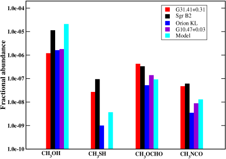
Figure 9: Comparison of abundance of CH₃OH, CH₃SH, CH₃CHO and CH₃NCO between G31 and other sources (Sgr B2, Orion KL, G10.47+0.03, and model). These abundances are given in the Table 4 with their references.

4 Discussions

Synthesis of many COMs (e.g., ethylene glycol, methyl formate, etc.) in G31 has been discussed by Rivilla et al. (2017). They discussed the formation routes of a few COMs. Thus, we do not concentrate on the synthesis of all the species which are identified in the present observation. Here, we mainly focus on the chemistry of two newly reported molecules, CH₃NCO and CH₃SH and two other COMs such as CH₃OH and CH₃OCHO that are discussed in the text. Here, we have discussed the possible synthesis routes of these species and compared their observed abundance/molecular ratio between G31 and other hot molecular cores. We have also shown a comparison between observed results and existing astrochemical simulation of these species. For the modeling results, we mainly followed Garrod et al. (2013). They considered an isothermal collapse phase, which is followed by a static warm-up phase. In the first phase, the density increases from $\rm{n_{H}=3\times 10^{3}}$ to $\rm{10^{7}\ cm^{-3}}$ under the free-fall collapse. At the initial phase, dust temperature falls to 8 K from 16 K. In the second phase; the temperature varies from 8 K to 400 K, where density remains fixed at $\rm{10^{7}\ cm^{-3}}$. The temperature of this source is $\sim$150 K, which is typical hot core temperature, and the number density ($\rm{n_{H}}$) of this source is $\sim$ $\rm{10^{7}\ cm^{-3}}$ (Beltrán et al., 2018). Thus, the hot core model of Garrod et al. (2013) is suitable for understanding chemical evolution of COMs in this source. They used three different warm-up models based on the time scale (i.e., fast, medium, and slow) and the final temperature of their model is much larger than one that is observed in this source. The timescale of the fast warm-up model is more suitable for studying the chemical evolution in high-mass star-forming regions. We used peak gas-phase abundances of all the species around 100-200 K of fast warm-up timescale model to compare with the observed values. Figure 9 compares the observed fractional abundance of CH₃OH, CH₃SH, CH₃OCHO, and CH₃NCO between G31 and other sources. The chemistry of these COMs is discussed in the following subsections.

4.1 CH₃OH and CH₃SH

CH₃OH and CH₃SH molecules are the chemical analog of each other and have a similar structure only difference is that one has an oxygen atom another sulfur atom. Emitting regions of CH₃SH transitions are compact and marginally resolved, whereas the emitting region of methanol is slightly extended compared to CH₃SH. A large number of previous experimental, theoretical, and observed results suggest that these two species are mainly produced on the grain surface via successive hydrogen addition reactions (e.g., Das et al., 2008; Fedoseev et al., 2015; Müller et al., 2016; Gorai et al., 2017; Vidal et al., 2017) with CO and CS, respectively. The main route of formation of methanol and methanethiol is given below,

CO $\xrightarrow{\text{H}}$ HCO $\xrightarrow{\text{H}}$ H₂CO $\xrightarrow{\text{H}}$ CH₃O $\xrightarrow{\text{H}}$ CH₃OH and CS $\xrightarrow{\text{H}}$ HCS $\xrightarrow{\text{H}}$ H₂CS $\xrightarrow{\text{H}}$ CH₃S $\xrightarrow{\text{H}}$ CH₃SH.

For the above reaction schemes, the first and third steps posses an activation barrier, whereas the second and fourth steps are barrier-less (e.g., Hasegawa et al., 1992; Gorai et al., 2017). At low-temperature regions, methanol and methanethiol are efficiently produced on the grain surface and released to the gas phase via non-thermal desorption in the cold phase and during the warm-up stage via thermal desorption process. From the astrochemical simulation, Müller et al. (2016) found that peak abundance of methanol arises around $130$ K. Here, our observed results of methanol predict the gas temperature $\sim 180$ K, which is similar to the typical hot core temperature. In addition to grain surface reactions, H₂CS can also be produced in the gas phase. In the gas phase, H₂CS is mainly produced from H₃CS⁺, where H₃CS⁺ is formed via the ion-neutral reaction between S⁺ and CH₄. Below $\sim$20 K with a density ($\rm{n_{H}}$) around $\rm{10^{4}-10^{5}\ cm^{-3}}$, H₂CS is accreted onto the grain surface directly from gas phase, which may also contribute to the CH₃SH formation (Bonfand et al., 2019).

The observed abundance of CH₃SH in G31 is $\rm{2.7\times 10^{-08}}$ and $\rm{1.0\times 10^{-09}}$ in Orion KL (Kolesniková et al., 2014, see Table 4). The observed abundance of methanethiol in Sgr B2 is $\sim$3.5 times higher than the G31. Methanol abundance is almost similar in G31, Orion KL, G10.47+0.03, and 10 times higher in Sgr B2 (see Figure 9). The observed CH₃SH/CH₃OH ratio in G31 is similar to Orion KL and it is eight times higher in Sgr B2. Modeling results of these two species also have comparable abundances and molecular ratio (see Table 4).

4.2 CH₃OCHO

Methyl formate can efficiently be produced on the surface of dust-grains through the reaction between methoxy radical (CH₃O) and formyl radical (HCO) (Garrod et al., 2008, 2013). Their simulation shows that, around 30-40 K, these radicals are mobile, and the reaction is efficient. It is clear from their simulation that gas phase CH₃OCHO is mainly coming from the ice phase (see Figure 1 of Garrod et al., 2013). Increased UV photodissociation of CH₃OH leads to the formation of various radicals CH₃, CH₃O, and CH₂O, around 40 K temperature, these are mobile and form the COMs (e.g., CH₃OCHO, CH₃OCH₃). In the gas phase, when T $\sim$ 40 K, protonated methanol and H₂CO (when it is abundantly released to the gas phase) react and form HC(OH)OCH₃⁺. Then electron recombination of HC(OH)OCH₃⁺ produce CH₃OCHO (Bonfand et al., 2019). An efficient gas-phase reaction of methyl formate production was proposed by Balucani et al. (2015) for the cold environment, where dimethyl ether is the precursor of methyl formate. Dimethyl ether is also present in this source (Isokoski, Bottinelli & van Dishoeck., 2013). Therefore methyl formate can be produced through both grain surface and gas-phase reactions. The observed abundance of CH₃OCHO in G31 is $\rm{4.25\times 10^{-7}}$, which is similar to the observed abundance in Sgr B2, G10.47+0.03 and ten times higher as compared to the Orion KL and modeling results. In G31, we have observed CH₃OCHO/CH₃OH abundance ratio $\sim$ 0.14-0.35. For other high-mass star-forming regions, this ratio is found to be $0.03$, $0.03$, and $0.08$ in Sgr B2, Orion KL, and G10.47+0.03, respectively (see Table 4).

4.3 CH₃NCO

In this work, we find emitting regions of CH₃NCO is compact. In this source, Rivilla et al. (2017) also observed a similar emitting region of ethylene glycol. It is primarily produced on the grain surface via recombination of two HCO radicals followed by successive hydrogen addition reactions (Coutens et al., 2017). In case of CH₃NCO formation, Halfen et al. (2015) proposed two routes (i) reaction between HNCO(HOCN) and CH₃, and (ii) reaction between HNCO(HOCN) and $\rm{CH_{5}^{+}}$. Cernicharo et al. (2016) proposed that it could be produced on the grain surface. The experiment result suggests that CH₃NCO can efficiently be produced on the solid phase through the reaction between CH₃ and (H)NCO (Ligterink et al., 2017). The hot core model suggests that it could be produced via a radical-radical reaction between CH₃ and OCN (Belloche et al., 2017). Since the reaction mentioned above is exothermic and barrier-less, it can efficiently be produced on the grain surface at a little warmer temperature ($>$30 K), when radical get enough mobility. Though CH₃NCO is efficiently produced on the grain surface, it could also be destructed by hydrogen addition reactions and produce n-methyl formamide (Belloche et al., 2017). Quénard et al. (2018) also considered similar radical-radical reactions in their chemical model to study the evolution of CH₃NCO under hot core conditions. In the hot core, when the temperature reaches around 100 K, CH₃ and HNCO can thermally desorb from the grain surface and increase the formation of CH₃NCO (Martín-Doménech et al., 2017; Gorai et al., 2020). Our estimated CH₃NCO abundance in G31 is $\sim$ $\rm{4.72\times 10^{-8}}$. For other hot molecular cores (e.g., Sgr B2, Orion KL), we have found a comparable abundance of CH₃NCO. The observed fractional abundance of CH₃NCO in this work is well within the modeled results (model 5) of Belloche et al. (2017).

The identification of CH₃OH, CH₃OCHO, CH₃NCO, and CH₃SH in G31 suggesting both grain surface and gas phase chemistry is efficient in this source for the formation of COMs. However, we can not distinguish the contribution from the gas and grain phase separately due to the observational limit. To explain the various observed line profile in this work, it requires a combined chemical and radiative transfer model, which will be carried out in our follow-up study.

5 Conclusions

We analyzed ALMA band 3 data of a hot molecular core, G31.41+0.31, and the following conclusions are made.

• We detected methyl isocyanate (CH₃NCO) and methanethiol (CH₃SH), for the first time in G31.
  

• We obtained two temperature components by using rotation diagram analysis. The cold component is obtained by CH₃OH and CH₃NCO where temperature varies between 33 and 48 K. Hot component is obtained by CH₃SH, CH₃OH and CH₃OCHO where the temperature ranges between 143 and 181 K. Estimated hydrogen ($\rm{N_{H_{2}}}$) column density is $\sim$ 1.53$\times 10^{25}$ cm^-2 and dust is optically thin at 94 GHz.
  

• We estimated column density and fractional abundances of various complex species CH₃NCO, CH₃SH, CH₃OH, and CH₃OCHO in G31. A comparison of column density/fractional abundances of these species between G31 and other hot molecular cores is discussed. We also compared our observed results with available chemical modeling under hot core conditions. Our observed abundances of COMs in G31 are consistent with other hot cores, Sgr B2, Orion KL, and G10.47+0.03, which suggests similar formation mechanisms of these complex species in these sources.
  

• For the kinematics of this source, a low excitation line of $\rm{H^{13}CO^{+}}$ is observed as an inverse P-Cygni profile, which suggests that there is an infall toward the center of this source, i.e., this source is in the younger stage of its evolution.
  

• Protostellar outflows are traced by SiO and HCN. Their blue-shifted and red-shifted emission clearly trace outflow along East-West direction. We estimated various outflow parameters. The average dynamical time scale of outflow is $\sim$ $10^{3}$ years.
  

6 Acknowledgement

This paper makes use of the following ALMA data: ADS/JAO.ALMA$\#$2015.1.01193.S. ALMA is a partnership of ESO (representing its member states), NSF (USA), and NINS (Japan), together with NRC (Canada), NSC, and ASIAA (Taiwan), and KASI (Republic of Korea), in cooperation with the Republic of Chile. The Joint ALMA Observatory is operated by ESO, AUI/NRAO, and NAOJ. We are grateful to the anonymous referee for numerous comments and suggestions, which improved the manuscript. PG acknowledges CSIR extended SRF fellowship (Grant No. 09/904 (0013) 2018 EMR-I) and and Chalmers Cosmic Origins postdoctoral fellowship. AD acknowledges ISRO respond project (Grant No. ISRO/RES/2/402/16-17) for partial financial support. B.B. acknowledges DST-INSPIRE Fellowship [IF170046] for providing partial financial assistance. SKM acknowledges CSIR fellowship (Ref no. 18/06/2017(i) EU-V). This work is partially supported by Consortium for the Development of Human Resources in Science and Technology by Japan Science and Technology Agency. This research was possible in part due to a Grant-In-Aid from the Higher Education Department of the Government of West Bengal. DS acknowledges ASIAA postdoctoral research fund and travel grant. AD and TS also acknowledge support from DST JSPS grant.

Appendix A Fitted spectra, LTE model spectra, moment maps, and schematic diagram of G31 based on present observation.

Appendix B Summary of the emitting regions of the observed species.

Table 6: Emitting region of observed transitions of COMs

Species	Transition	Emitting	Upper State
	Frequency	region	Energy
	(GHz)	(′′)	(K)
CH3SH	101.13915a	0.89$\pm$0.06	12.14
	101.15999b	0.80$\pm$0.02	52.39
	101.16830c	0.80$\pm$0.05	30.27
CH3OH	86.61557	1.35$\pm$0.01	102.70
	86.90291	1.35$\pm$0.02	102.72
	88.59478	1.29$\pm$0.02	328.28
	88.93997	1.27$\pm$0.01	328.28
	101.12685	1.14$\pm$0.03	60.73
	101.29341	1.21 $\pm$0.02	90.91
	101.46980	1.23 $\pm$0.03	109.49
CH3NCO	86.68019	0.82$\pm$0.01	22.82
	86.68655	0.83$\pm$0.02	34.97
	86.78077	0.78$\pm$0.02	46.73
	86.80502	0.77$\pm$0.01	46.74
	87.01607	0.76$\pm$0.02	58.88
CH3OCHO	88.6869	1.37$\pm$0.04	44.97
	88.72326	1.10$\pm$0.03	44.96
	88.84318	1.36$\pm$0.02	17.96
	88.85160	1.42$\pm$0.02	17.94
	88.86241	1.15$\pm$0.04	207.10
	101.37054	1.46$\pm$0.05	59.64
	101.41474	1.33$\pm$0.06	59.63
SO2	86.63908	0.71$\pm$0.01	55.20
H2CO	101.33299	1.31$\pm$0.02	87.57

NOTES: ^a multiple transitions: 101.13915/101.13965 GHz, ^b multiple transitions: 101.15999/101.15933/101.16066/101.16069 GHz, ^c multiple transitions: 101.16715/101.16830 GHz.

References

- Araya et al. (2008) Araya, E., Hofner, P., Kurtz, P., Olmi, L. & Linz, H, 2008, ApJ, 675, 420
- Altwegg et al. (2017) Altwegg K., Balsiger, H., Berthelieret, J. J. et al. 2017, MNRAS, 469, S130
- Estalella et al. (2019) Estalella, R., Anglada, G., Díaz-Rodríguez, A. K., Mayen-Gijon, J. M. 2019, A&A, 626, A84
- Balucani et al. (2015) Balucani N., Ceccarelli C., Taquet V. 2015, MNRAS, 449, L16
- Belloche et al. (2008) Belloche, A., Menten, K. M., Comito, C. et al. 2008, A&A, 482, 179
- Belloche et al. (2013) Belloche, A., Müller, H. S. P., Menten, K. M. et al. 2013, A&A, 559, A47
- Belloche et al. (2014) Belloche, A., Garrod, R.T. , Müller, H. S. P., & Menten, K. M. 2014, Science, 345, 158
- Belloche et al. (2016) Belloche, A., Müller, H. S. P., Garrod, R. T., & Menten, K. M. 2016, A&A, 587, A91
- Belloche et al. (2017) Belloche, A., Meshcheryakov, A. A., Garrodet, R. T. et al. 2017, A&A, 601, A49
- Beltrán et al. (2005) Beltrán M. T., Cesaroni R., Neri R. et al. 2005, A&A, 435, 90
- Beltrán et al. (2009) Beltrán, M.T., Codella, C., S. Viti, S. et al. 2009, 690, L93
- Beltrán & de Wit (2016) Beltrán, M. T. & de Wit, W. J. 2016, A&A Rev., 24, 6
- Beltrán et al. (2018) Beltrán, M. T., Cesaroni, R., Rivilla, V. M. et al. 2018, A&A, 615,141
- Beltrán et al. (2019) Beltrán et al. 2019, A&A, 630, 54
- Black et al. (1987) Blake, G. A., Sutton, E., Masson, C., & Phillips, T. 1987, ApJ, 315, 621
- Boehler et al. (2017) Boehler, Y., Weaver, E., Isella, A., et al. 2017, ApJ, 840, 60
- Bonfand et al. (2017) Bonfand, M., Belloche, A., Menten, K. M. et al. 2017, A&A, 604, 60
- Bonfand et al. (2019) Bonfand, M., Belloche, A., Garrod, R.T., et al. A&A, 628, A27
- Brown et al. (1975) Brown, R.D., Crofts, J.G., Godfrey, P.D. et al. 1975, ApJ, 197, L29.
- Cabrit & Bertout. (1990) Cabrit, S., & Bertout, C. 1992, A&A, 261, 276
- Calmonte et al. (2016) Calmonte, U., Altwegg, K., Balsiger, H. et al. 2016, MNRAS, 462, S253
- Casassus et al. (2013) Casassus, S., van der Plas, G., M, S. P., et al. 2013, Nature, 493, 191
- Cazaux et al. (2003) Cazaux, S., Tielens, A. G. G. M., Ceccarelli, C. et al. 2003, ApJ. 593, L51
- Cernicharo et al. (2016) Cernicharo J., Kisiel, Z., Tercero, B., et al., 2016, A&A, 587, L4
- Cesaroni et al. (2010) Cesaroni, R., Hofner, P., Araya, E., & Kurtz, S. 2010, A&A, 509, 50
- Cesaroni et al. (2011) Cesaroni, R., Beltrán, M. T., Zhang, Q. et al. 2011, A&A, 533, A73
- Cesaroni et al. (2017) Cesaroni, R., Sánchez-Monge, Á., Beltrán, M. T., et al. 2017, A&A, 602, A59
- Charnley et al. (1997) Charnley, S. B. 1997, ApJ, 481, 396
- Chakrabarti et al. (2015) Chakrabarti, S.K., Majumdar, L., Das, A., Chakrabarti, S., 2015, APSS, 2015, 357, 90
- Churchwell et al. (1990) Churchwell E., Walmsley C. M., Cesaroni R., 1990, A&AS, 83, 119
- Coutens et al. (2017) Coutens, A., Viti, S., Rawlings, J.M.C. et al. 2017, MNRAS, 475, 2016
- Codella et al. (2013) Codella, C., Beltrán, M. T., Cesaroni, R., et al. 2013, A&A, 550, A81
- Cox et al. (2000) Cox, A. N. 2000, Allen’s Astrophysical Quantities (New York: AIP Press)
- Daly et al. (2013) Daly, A., Bermúdez, C., López, A. et al. 2013, ApJ, 768, 81
- Das et al. (2008) Das, A., Acharyya, K., Chakrabarti, S. & Chakrabarti, S. K. 2008b, A&A, 486, 209
- Das et al. (2010) Das, A., Acharyya, K. & Chakrabarti, S. K., 2010, MNRAS 409, 789
- Das & Chakrabarti (2011) Das, A. & Chakrabarti, S. K., 2011, MNRAS, 418, 545
- Das et al. (2016) Das, A., Sahu, D., Majumdar, L., & Chakrabarti, S. K., 2016, MNRAS, 455, 540.
- Demyk et al. (2007) Demyk, K., Mäder, H.; Tercero, B. et al. 2007, A&A, 466, 255
- Di Francesco et al. (2001) Di Francesco, J., Myers, P. C., Wilner, D. J. et al. 2001, ApJ, 562, 770
- Esplugues et al. (2013) Esplugues, G. B., Tercero, B., Cernicharo, J., et al. 2013, A&A, 556, A143
- Favre et al. (2011) Favre, C., Despois, D., Brouillet, N., et al. 2011, A&A, 532, A32
- Favre et al. (2015) Favre, C., Bergin, E. A., Neill, J. L., et al. 2015, ApJ, 808, 155
- Fedoseev et al. (2015) Fedoseev, G., Cuppen, H. M., Ioppolo, S., Lamberts, T., & Linnartz, H. 2015, MNRAS, 448, 1288
- Garrod et al. (2008) Garrod R. T., Weaver S. L. W., Herbst E., 2008, ApJ, 682, 283
- Garrod et al. (2013) Garrod R. T., 2013, ApJS, 765, 60
- Gibb et al. (2000) Gibb, E., Nummelin, A., Irvine, W. M. et al. 2000, ApJ, 545, 309
- Girart et al. (2009) Girart, J. M., Beltrán, M. T., Zhang, Q. et al. 2009, Science, 324, 1408
- Girart et al. (2018) Girart, J. M., Fernández-López, M., Li, Z. -Y., et al. 2018, ApJL, 856, L27
- Goesmann et al. (2015) Goesmann F. et al., 2015, Science, 346, 6247
- Gorai et al. (2017) Gorai, P., Das, A., Das, A., et al. 2017, ApJ, 836, 70
- Gorai et al. (2020) Gorai, P., Bhat, B., Sil, M., Mondal, S. K., Ghosh, R., Das, A., 2020, ApJ, 895, 86
- Goldsmith & Langer. (1999) Goldsmith, P. F., & Langer, W. D. 1999, ApJ, 517, 209
- Halfen et al. (2015) Halfen D. T., Ilyushin V. V., Ziurys L. M., 2015, ApJ, 812, L5
- Hasegawa et al. (1992) Hasegawa, T. I., Herbst, E. & Leung, C. M. 1992, ApJS, 82, 167
- Herbst & van Dishoeck (2009) Herbst, E. & van Dishoeck, E. F. 2009, ARA&A, 47, 427
- Higuchi et al. (2015) Higuchi, A. E., Hasegawa, T., Saigo, K. et al. J. O. 2015, ApJ, 815, 106
- Hollis et al. (2004) Hollis, J, M., Jewell., P.R., Lovas, F.J.,& Remijan, A. 2004, ApJ, 613, L45
- Isella et al. (2016) Isella, A., Guidi, G., Testi, L., et al. 2016, PhRvL, 117, 25
- Isokoski, Bottinelli & van Dishoeck. (2013) Isokoski K., Bottinelli S., van Dishoeck E. F., 2013, A&A, 554, A100
- Jin et al. (2016) Jin, S., Li, S., Isella, A., Li, H., & Ji, J. 2016, ApJ, 818, 76
- Kolesniková et al. (2014) Kolesniková, L., Tercero, B., Cernicharo, J., et al. 2014, ApJ, 784, L7
- Kraus et al. (2010) Kraus, S., Hofmann, K-H., Menten, K. M., et al. 2010, Nature, 466, 339
- Kurtz et al. (2000) Kurtz S., Cesaroni R., Churchwell E. et al. 2000, Protostars and Planets IV ed V. Mannings, A. P. Boss and S. S. Russell (Tucson, AZ: Univ. Arizona Press) 299
- Leurini et al. (2007) Leurini, S., Beuther, H., Schilke, P. et al. 2007, A&A, 475, 925
- Leurini et al. (2014) Leurini, S., Codella, C., López-Sepulcre, A. et al. 2014, A&A, 570, A49
- Ligterink et al. (2015) Ligterink, N. F. W, Tenenbaum, E. D., & van Dishoeck, E. F, 2015, A&A, 576, A35
- Ligterink et al. (2017) Ligterink N. F. W., et al., 2017, MNRAS, 469, 2219
- Linke et al. (1979) Linke, R. A., Frerking, M. A., & Thaddeus, P., 1979, ApJ, 234, L139
- Majumdar et al. (2015) Majumdar, L., Gorai, P., Das, Ankan., Chakrabarti, S. K., 2015, APSS, 360, 64
- McGuire et al. (2016) McGuire, B. A., Carroll, P. B., Loomis, R. A. et al. 2016, Science, 352, 1449-1552.
- McMullin et al. (2007) McMullin, J. P., Waters, B., Schiebel, D., Young, W., & Golap, K. 2007, Astronomical Data Analysis Software and Systems XVI (ASP Conf. Ser. 376), ed. R. A. Shaw, F. Hill, & D. J. Bell (San Francisco, CA: ASP), 127
- Margulés et al. (2016) Margulés, L, Belloche, A., Müller, H.S.P., Motiyenko, R. A. et al. A&A, 2016
- Martín-Doménech et al. (2017) Martín-Doménech, R., Rivilla, V. M., Jiménez-Serra, I., et al. 2017, MNRAS, 469, 2230
- Müller et al. (2016) Müller, H.S.P., Belloche, A., Xu, L. et al. 2016, A&A, 587, A92
- Müller et al. (2008) Müller, H. S. P., Belloche, A., Menten, K. M., et al. 2008, J. Mol. Spectr., 251, 319
- Müller et al. (2001) Müller, H. S. P., Thorwirth, S., Roth, D. A., & Winnewisser, G. 2001, A&A 370, L49
- Müller et al. (2005) Müller, H. S. P., Schlöder, F., Stutzki, J., & Winnewisser, G. 2005, J. Mol. Str, 742, 215
- Mayen-Gijon et al. (2014) Mayen-Gijon, J. M. Anglada, G., Osorio, M., et al. 2014, MNRAS, 437, 3766
- Öberg et al. (2011) Öberg K. I., Boogert A. C. A., Pontoppidan K. M., et al. eds, IAU Symposium Vol. 280, 2011, The Molecular Universe. pp 65– (arXiv:1107.5826), doi:10.1017/S1743921311024872
- Ossenkopf & Henning (1994) Ossenkopf, V., & Henning, T. 1994, A&A, 291, 943
- Olmi et al. (1996) Olmi, L., Cesaroni, R., & Walmsley, C. M. 1996, A&A, 307, 599
- Oya et al. (2016) Oya, Y., Nami Sakai, N., López-Sepulcre, A. et al. 2016, ApJ, 824, 88
- Osorio et al. (2009) Osorio, M., Anglada, G., Lizano, S. et al. 2009, ApJ, 694, 29.
- Patel et al. (2005) Patel, N. A., Curiel, S., Sridharan, T. K et al. 2005, Nature, 437, 109
- Pickett et al. (1998) Pickett, H. M., Poynter, R. L., Cohen, E. A. et al. 1998, JQSRT, 60, 883
- Pirogov et al. (1997) Pirogov, L., Zinchencko, I., Lapinov, A. et al. 1995, A&AS, 09, 333
- Quénard et al. (2018) Quénard, D., Jiménez-Serra, I., Viti, S.,et al. 2018, MNRAS, 474, 2796
- Ried et al. (2019) Reid, M., et al. 2019, ApJ, 885, 131
- Rivilla et al. (2017) Rivilla, V.M., Beltrán, M.T., Cesaroni, R. et al. 2017, A&A, 598, 59
- Rolffs et al. (2011) Rolffs, R., Schilke, P., Zhang, Q., & Zapata, L., 2011, A&A, 536, A33
- Schilke et al. (2001) Schilke, P., Benford, D. J., Hunter, T. R. et al. 2001, ApJS, 132, 281
- Sahu et al. (2018) Sahu, D., Minh., Y.C., Lee, C-F. et al. 2018, MNRAS, 475, 5322
- Sahu et al. (2020) Sahu, D., Liu, S-Y., Das, A., et al. 2020, ApJ, 899, 65
- Sil et al. (2018) Sil, M., Gorai, P., Das, A. et al. ApJ, 2018, 853, 2
- Snyder & Buhl. (1971) Snyder, L. E., & Buhl, D. 1971, ApJ. 163, L47
- Sutton et al. (1995) Sutton, E. C., Peng, R., Danchi, W.C. et al. 1995, ApJS, 97, 455
- Tan et al. (2014) Tan, J. C., Beltrán, M. T., Caselli, P. et al. 2014, Protostars and Planets VI, 149
- Tercero et al. (2018) Tercero, B., Cuadrado, S., López, A., et al. 2018, A&A, 620, L6
- Vidal et al. (2017) Vidal, T. H. G., Loison, J-C., Jaziri, A. Y., et al. 2017, MNRAS, 469, 435
- van Dishoeck & Black et al. (1998) van Dishoeck E. F., Blake G. A. 1998, Annu Rev Astron Astrophys, 36, 317
- Van der Tak et al. (2007) Van der Tak, F. F. S., Black, J. H., Schöier, et al. 2007, A&A 468, 627
- Van der Marel et al. (2016) van der Marel, N., van Dishoeck, E. F., Bruderer, S., et al. 2016, A&A 585, A58
- Weaver et al. (2018) Weaver, E., Isella, A., & Boehler, Y. 2018, ApJ, 853, 113
- Whittet (1992) Whittet, D. C. B. 1992, Dust in the Galactic Environment (Bristol: IOP Publishing)
- Ziurys & Turner. (1986) Ziurys, L. M., & Turner, B. E. 1986, ApJ, 300, L19
- Zapata et al. (2009) Zapata, L. A., Ho, P. T. P., Schilke, P. et al. 2009, ApJ, 698, 1422