Improving the Performance of the GMRES Method using Mixed-Precision Techniques

Abstract

The GMRES method is used to solve sparse, non-symmetric systems of linear equations arising from many scientific applications. The solver performance within a single node is memory bound, due to the low arithmetic intensity of its computational kernels. To reduce the amount of data movement, and thus, to improve performance, we investigated the effect of using a mix of single and double precision while retaining double-precision accuracy. Previous efforts have explored reduced precision in the preconditioner, but the use of reduced precision in the solver itself has received limited attention. We found that GMRES only needs double precision in computing the residual and updating the approximate solution to achieve double-precision accuracy, although it must restart after each improvement of single-precision accuracy. This finding holds for the tested orthogonalization schemes: Modified Gram-Schmidt (MGS) and Classical Gram-Schmidt with Re-orthogonalization (CGSR). Furthermore, our mixed-precision GMRES, when restarted at least once, performed 19% and 24% faster on average than double-precision GMRES for MGS and CGSR, respectively. Our implementation uses generic programming techniques to ease the burden of coding implementations for different data types. Our use of the Kokkos library allowed us to exploit parallelism and optimize data management. Additionally, KokkosKernels was used when producing performance results. In conclusion, using a mix of single and double precision in GMRES can improve performance while retaining double-precision accuracy.

1 Introduction

The gmres method [22] is used for solving sparse, non-symmetric systems of linear equations arising from many applications [21, p. 193]. It is an iterative, Krylov subspace method that constructs an orthogonal basis by Arnoldi’s procedure [2] then finds the solution vector in that subspace such that the resulting residual is minimized. One important extension of gmres is the introduction of restarting, whereby, after some number of iterations, gmres computes the solution vector, then starts over with an empty Krylov subspace and the newly computed solution vector as the new initial guess. This limits the number of basis vectors required for the Krylov subspace thus reducing storage and the computation needed to orthogonalize each new vector. On a single node system, performance of gmres is bound by the main memory bandwidth due to the low arithmetic intensity of its computational kernels. We investigated the use of a mix of single and double floating-point precision to reduce the amount of data that needs to be moved across the cache hierarchy, and thus improve the performance, while trying to retain the accuracy that may be achieved by a double-precision implementation of gmres. We utilized the iterative nature of gmres, particularly when restarted, to overcome the increased round-off errors introduced by reducing precision for some computations.

The use of mixed precision in solving linear systems has long been established in the form of iterative refinement for dense linear systems [24], which is an effective tool for increasing performance [6]. However, research to improve the performance of gmres in this way has had limited scope. One similar work implemented iterative refinement with single-precision Krylov solvers, including gmres, to compute the error corrections [1]. However, that work did not explore the configuration of gmres and tested only a limited set of matrices. Recent work by Gratton et al. provides detailed theoretical results for mixed-precision gmres [12]; although, they focus on non-restarting gmres and understanding the requirements on precision for each inner-iteration to converge as if done in uniform, high precision. Another approach is to use reduced precision only for the preconditioner [10]. One interesting variant of reduced-precision preconditioners is to use a single-precision gmres to precondition a double-precision gmres [3].

In this paper, we focus on restarted gmres with left preconditioning and with one of two orthogonalization schemes: mgs or cgsr, as shown in Alg. 1. The algorithm contains the specifics of the gmres formulation that we used.

Algorithm 1 Restarted GMRES with left preconditioning [21]

1:$\tens{A}\in\mathbb{R}^{n\times n},\quad\vec{x_{0}},\vec{b}\in\mathbb{R}^{n},\quad\tens{M}^{-1}\approx\tens{A}^{-1}$

2:for $k=1,2,\dots$ do

3:     $\vec{z_{k}}\leftarrow\vec{b}-\tens{A}\vec{x_{k}}$ $\triangleright$ compute residual

4:     If $\|\vec{z_{k}}\|_{2}$ is small enough, stop

5:     $\vec{r_{k}}\leftarrow\tens{M}^{-1}\vec{z_{k}}$

6:     $\beta\leftarrow\|\vec{r_{k}}\|_{2},\quad s_{0}\leftarrow\beta,\quad\vec{v_{1}}\leftarrow\vec{r}_{k}/\beta,\quad\tens{V_{1}}\leftarrow[\vec{v_{1}}]$

7:     $j\leftarrow 0$

8:     loop until the restart condition is met

9:         $j\leftarrow j+1$

10:         $\vec{w}\leftarrow\tens{M}^{-1}\tens{A}\vec{v_{j}}$

11:         $\vec{w},h_{1,j},\dots,h_{j,j}\leftarrow\mathrm{orthogonalize}(\vec{w},\tens{V_{j}})$ $\triangleright$ mgs or cgsr

12:         $h_{j+1,j}\leftarrow\|\vec{w}\|_{2}$

13:         $\vec{v_{j+1}}\leftarrow\vec{w}/h_{j+1,j}$

14:         $\tens{V_{j+1}}\leftarrow[\tens{V_{j}},\vec{v_{j+1}}]$

15:         for $i=1,\dots,j-1$ do

16:              $\begin{bmatrix}h_{i,j}\\ h_{i+1,j}\end{bmatrix}\leftarrow\begin{bmatrix}\alpha_{i}&\beta_{i}\\ -\beta_{i}&\alpha_{i}\end{bmatrix}\times\begin{bmatrix}h_{i,j}\\ h_{i+1,j}\end{bmatrix}$ $\triangleright$ apply Givens rotation

17:         end for

18:         $\begin{bmatrix}\alpha_{j}\\ \beta_{j}\end{bmatrix}\leftarrow\text{{rotation\_matrix}}\left(\begin{bmatrix}h_{j,j}\\ h_{j+1,j}\end{bmatrix}\right)$ $\triangleright$ form $j$-th Givens rotation

19:         $\begin{bmatrix}s_{j}\\ s_{j+1}\end{bmatrix}\leftarrow\begin{bmatrix}\alpha_{j}&\beta_{j}\\ -\beta_{j}&\alpha_{j}\end{bmatrix}\times\begin{bmatrix}s_{j}\\ 0\end{bmatrix}$

20:         $\begin{bmatrix}h_{j,j}\\ h_{j+1,j}\end{bmatrix}\leftarrow\begin{bmatrix}\alpha_{j}&\beta_{j}\\ -\beta_{j}&\alpha_{j}\end{bmatrix}\times\begin{bmatrix}h_{j,j}\\ h_{j+1,j}\end{bmatrix}$

21:     end loop

22:     $\tens{H}\leftarrow\{h_{i,\ell}\}_{1\leq i,\ell\leq j},\quad\vec{s}\leftarrow[s_{1},\dots s_{j}]^{T}$

23:     $\vec{u_{k}}\leftarrow\tens{V_{j}}\tens{H}^{-1}\vec{s}$ $\triangleright$ compute correction

24:     $\vec{x_{k+1}}\leftarrow\vec{x_{k}}+\vec{u_{k}}$ $\triangleright$ apply correction

25:end for

26:

27:procedure mgs($\vec{w},\tens{V_{j}}$)

28:     $[\vec{v_{1}},\dots,\vec{v_{j}}]\leftarrow\tens{V_{j}}$

29:     for i = 1, 2, …, j do

30:         $h_{i,j}\leftarrow\vec{w}\cdot\vec{v_{i}}$

31:         $\vec{w}\leftarrow\vec{w}-h_{i,j}\vec{v_{i}}$

32:     end for

33:     return $\vec{w},h_{1,j},\dots,h_{j,j}$

34:end procedure

35:

36:procedure cgsr($\vec{w},\tens{V_{j}}$)

37:     $\vec{h}\leftarrow\tens{V_{j}}^{T}\vec{w}$

38:     $\vec{w}\leftarrow\vec{w}-\tens{V_{j}}\vec{h}$

39:     $[h_{0,j},\dots,h_{j,j}]^{T}\leftarrow\vec{h}$

40:     return $\vec{w},h_{1,j},\dots,h_{j,j}$

41:end procedure

mgs is the usual choice for orthogonalization in gmres due to its lower computational cost compared to other schemes [20]. cgsr is used less often in practice but differs in interesting ways from mgs. First, it retains good orthogonality relative to round-off error [11], which raises the question of whether this improved orthogonality can be used to circumvent some loss of precision. Second, it can be implemented as matrix-vector multiplies, instead of a series of dot-products used by mgs. Consequently, cgsr requires fewer global reductions and may be a better candidate when considering expanding the work to a distributed memory setting. Restarting is used to limit the storage and computation requirements of the Krylov basis generated by gmres [4, 5].

2 Numerics of Mixed Precision gmres

To use mixed precision for improving the performance of gmres, it is important to understand how the precision of different parts of the solver affects the final achievable accuracy. First, for the system of linear equations $\tens{A}\vec{x}=\vec{b}$; $\tens{A}$, $\vec{b}$, and $\vec{x}$ all must be stored in full precision because changes to these values change the problem being solved and directly affect the backward and forward error bounds. Next, note that restarted gmres is equivalent to iterative refinement where the error correction is computed by non-restarted gmres. Hence, adding the error correction to the current solution must be done in full precision to prevent $\vec{x}$ from suffering round-off to reduced precision. Additionally, full precision is critical for the computation of residual $\vec{r}=\tens{A}\vec{x}-\vec{b}$ because it is used to compute the error correction and is computed by subtracting quantities of similar value. Were the residual computed in reduced precision, the maximum error that could be corrected is limited by the accuracy used for computing the residual vector [7].

Next, consider the effects of reducing precision in the computation of the error correction. Note that for stationary iterative refinement algorithms, it has long been known that reduced precision can be used in this way while still achieving full accuracy [24], which, to some extent, can be carried over to the non-stationary correction of gmres. The converge property derives from the fact that if each restart ${i=1,\dots,k}$ computes an update, $\vec{u}_{i}$, fulfilling ${\|\vec{r}_{i}\|}={\|\vec{r}_{i-1}-\tens{A}\vec{u}_{i}\|}\leq{\delta\|\vec{r}_{i-1}\|}$ for some error reduction $\delta<1$, then after $k$ steps we get ${\|\vec{r}_{k}\|}\leq{\delta^{k}\|\vec{r}_{0}\|}$ [1]. Thus, reducing the accuracy of the error-correction to single precision does not limit the maximum achievable accuracy. Furthermore, under certain restrictions on the round-off errors of the performed operations, non-restarted gmres behaves as if the arithmetic was done exactly [12]. Therefore, when restarted frequently enough, we hypothesize that mixed-precision gmres should behave like the double-precision implementation.

3 Restart Strategies

Restart strategies are important to the convergence. In cases when limitations of the memory use require a gmres restart before the accuracy in working precision is reached, the restart strategy needs no further consideration. However, if mixed-precision gmres may reach the reduced precision’s accuracy before the iteration limit, it is important to have a strategy to restart early. But restarting too often will reduce the rate of convergence because improvement is related to the Arnoldi process’s approximation of the eigenvalues of $\tens{A}$, which are discarded when gmres restarts [23]. As a countermeasure, we propose four possible approaches for robust convergence monitoring and restart initiation.

There are two points to note before discussing specific restart strategies. First, the choice of orthogonalization scheme is important to consider, because some Krylov basis vectors usually become linearly dependent when gmres reaches the working precision accuracy, e.g., mgs [20], while other methods remain nearly orthogonal, e.g., cgsr [11]. Second, the norm of the Arnoldi residual, the residual for gmres’s least-squares problem, approximates the norm of the residual of the original preconditioned linear system of equations and is computed every iteration when using Givens rotations to solve the least-squares problem ($s_{j+1}$ in Alg. 1) [21, Proposition 6.9]. However, this approximation only monitors the least-squares problem and is not guaranteed to be accurate after reaching working precision [13]. The explanation is unknown, but it has been noted that the Arnoldi residual typically decreases past the true residual if and only if independent vectors continue to be added to the Krylov basis. Hence, the choice of orthogonalization scheme must be considered when using restarts based on the Arnoldi residual norm.

Our first restart strategy derives from the observation that the number of iterations before the convergence stalls appears to be roughly constant after each restart. See Sec. 4.1 for numerical examples. While this does not alleviate the issue determining the appropriate point for the first restart, this can be used for subsequent restarts either to trigger the restart directly or as a heuristic for when to start monitoring other, possibly expensive, metrics.

The second restart strategy is to monitor the approximate preconditioned residual norm until it drops below a given threshold, commonly related to the value after the prior restart. The simplest threshold is a fixed, scalar value. Note that if the approximated norm stops decreasing, such as for mgs, this criterion will not be met until gmres is restarted. Thus, the scalar thresholds must be carefully chosen when using mgs. More advanced threshold selection may be effective, but we have not explored any yet.

Inspired by the problematic case of the second strategy, the third strategy is to detect when the Arnoldi residual norm stops improving. Obviously, this approach is only valid if the norm stops decreasing when gmres has stalled. Additionally, gmres can stagnate during normal operation, resulting in iterations of little or no improvement, which may cause premature restarts.

The final strategy is to detect when the orthogonalized basis becomes linearly dependent. This relates to the third strategy but uses a different approach. For the basis matrix $\tens{V}_{k}$ computed in the $k$th inner iteration, let $\tens{S}_{k}=(\tens{I}+\tens{U}_{k})^{-1}\tens{U}_{k}$, where $\tens{U}_{k}$ is the strictly upper part of $\tens{V}_{k}^{H}\tens{V}_{k}$ [18]. Then, the basis is linearly dependent if and only if $\|\tens{S}_{k}\|_{2}=1$. It has been conjectured that mgs-gmres converges to machine precision when the Krylov basis loses linear independence [20, 19]. This matrix can be computed incrementally, appending one column per inner iteration, requiring $2nk+2k^{2}$ FLOP per iteration. Estimating the 2-norm for a gmres-iteration with $i$ iterations of the power method requires an additional $i(2k^{2}+3k)$ FLOP by utilizing the strictly upper structure of the matrix.

4 Experimental Results

First, Sec. 4.1 shows accuracy and rate of convergence results to verify the results in Sec. 2 and to better understand the strategies proposed in Sec. 3. Next, Sec. 4.2 compares the performance of our mixed-precision approach and double-precision gmres. Based on the results in Sec. 2, we focused on computing the residual and updating $\vec{x}$ in double-precision and computing everything else in single-precision. This choice of precisions has the advantage that it can be implemented using uniform-precision kernels and only casting the residual to single-precision and the error-correction back to double precision. Note that in this approach, the matrix is stored twice, once in single-precision and once in double-precision; this storage requirement may be able to be improved by storing the high-order and low-order bytes of the double-precision matrix in separate arrays [14].

Matrices were stored in Compressed Sparse Row format and preconditioned with incomplete LU without fill in. So, the baseline, double-precision solver requires $24n_{nz}+8nm+28n+8m^{2}+O(m)$ bytes while the mixed-precision solver requires $24n_{nz}+4nm+32n+4m^{2}+O(m)$ where $n_{nz}$ is the number of matrix nonzero elements, $n$ is the number of matrix rows, and $m$ is the maximum number of inner iterations per restart. All of the tested matrices came from the SuiteSparse collection [8] and entries of the solution vectors were independently drawn from a uniform distribution between 0 and 1.

We used two implementations of gmres: a configurable one for exploring the effect various factors have on the rate of convergence, and an optimized one for testing a limited set of factors for performance. Both implementations are based on version 2.9.00 of the Kokkos performance portability library [9]. The OpenMP backend was used for all tests. Furthermore, for performance results we used the KokkosKernels library, with Intel’s MKL where supported, to ensure that improvements are compared against a state-of-the-art baseline. The rate of convergence tests were implemented using a set of custom, mixed-precision kernels for ease of experimentation.

All experiments were run on a single node with two sockets, each containing a ten-core Haswell processor, for a total of twenty-cores and $25\text{\,}\mathrm{MiB}$ of combined Level 3 cache. Performance tests were run with Intel C++ Compiler version 2018.1, Intel MKL version 2019.3.199, and Intel Parallel Studio Cluster Edition version 2019.3. The environment variables controlling OpenMP were set to: OMP_NUM_THREADS=20, OMP_PROC_BIND=spread, and OMP_PROC_BIND=places.

4.1 Measurement of the Rate of Convergence

To verify the analysis of Sec. 2, we first demonstrate that each variable behaves as predicted when stored in single-precision, while the rest of the solver components remain in double-precision. Figure 1 shows the normwise backward error after each inner iteration as if the solver had terminated, for gmres solving a linear system for the airfoil_2d matrix.

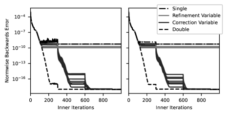
Figure 1: Rate of convergence results for the airfoil_2d matrix when restarting every 300 iterations for mgs (left) and cgsr (right) orthogonalization schemes

This matrix has $14\,214$ rows, $259\,688$ nonzeros, and a condition of $1.8\text{\times}{10}^{6}$. In the figure, the “Refinement Variables” include the matrix when used for the residual, the right-hand side, the solution, and the vector used to compute the non-preconditioned residual; the “Correction Variables” include the matrix when used to compute the next Krylov vector, the non-preconditioned residual, the Krylov vector being orthogonalized, the orthogonal basis, the upper triangular matrix from the orthogonalization process, and the vectors to solve the least-squares problems with Givens rotations. The convergence when storing the preconditioner in single-precision was visually indistinguishable from the double-precision baseline and omitted from the figure for the sake of clarity. Each solver was restarted after 300 iterations. All of the solvers behaved very similarly until single-precision accuracy was reached, where all of the solvers, except double-precision, stopped improving. After restarting, the solvers with reduced precision inside the error correction started improving again and eventually reached double-precision accuracy; however, the solvers with reduced precision in computing the residual or applying the error correction were unable to improve past single-precision accuracy.

The convergence test was repeated with two mixed-precision solvers that use reduced precision for multiple variables. The first used double precision only for computing the residual and error correction, i.e., using single precision for lines 4-23 of Alg. 1. The second was more limited, using single precision only to store $\tens{A}$ for computing the next Krylov vector, the preconditioner $\tens{M}^{-1}$, and the Krylov basis $\tens{V_{j}}$ from Alg. 1; these three variables make up most of the data that can be stored in reduced precision. Figure 2 shows the normwise backward error after each inner iteration for single, double, and mixed precisions solving a linear system for the airfoil_2d matrix.

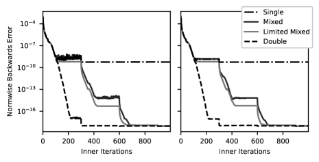
Figure 2: Rate of convergence results for the airfoil_2d matrix when restarting every 300 iterations for mgs (left) and cgsr (right) orthogonalization schemes

After restarting, both mixed-precision gmres implementations were able to resume improvement and achieve double-precision accuracy. This ability to converge while using reduced precision occurred for all of the matrices tested, as can be seen in Sec. 4.2. Note that while limiting the use of mixed precision can increase the amount of improvement achieved before stalling, this improvement is limited and does not reduce the importance of appropriately restarting. Additionally, the limited mixed-precision implementation requires several mixed-precision kernels, while the fully mixed-precision implementation can be implemented using uniform-precision kernels by copying the residual to single-precision and copying the error-correction back to double-precision.

One interesting observation was that the number of iterations before improvement stalled was approximately the same after each restart. Table 1 displays the number of iterations before stalling after the first three restarts in the mixed-precision mgs-gmres.

Table 1: Number of iterations before the improvement stalls in mixed-precision mgs-gmres

	Iterations	Iterations	Iterations	Iterations
Matrix	per Restart	for 1st Stall	for 2nd Stall	for 3rd Stall
airfoil_2d	300	137	141	142
big	500	360	352	360
cage11	20	7	7	8
Goodwin_040	1250	929	951	924
language	75	23	21	21
torso2	50	28	27	25

Stalling was defined here to be the Arnoldi residual norm improving by less than a factor of $1.001$ on the subsequent 5% of inner iterations per restart. This behavior appears to hold for cgsr too but was not quantified because stalled improvement cannot be detected in the Arnoldi residual for cgsr.

Next, restart strategies based on the Arnoldi residual norm were tested. First, Fig. 3 shows the convergence when restarted after a fixed improvement.

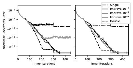
Figure 3: Rate of convergence results for the airfoil_2d matrix when restarting mixed-precision gmres after a fixed improvement in the Arnoldi residual norm for mgs (left) and cgsr (right) orthogonalization schemes, with vertical ticks to indicate when restarts occurred

Note that for mgs, when the threshold is too ambitious, mixed-precision gmres will stall because of roundoff error before reaching the threshold, at which point the approximated norm stops decreasing. However, the choice of restart threshold becomes problematic when considering multiple matrices. Figure 4 shows the same test applied to the big matrix, which has $13\,209$ rows, $91\,465$ nonzeros, and an L2 norm of $4.4\text{\times}{10}^{7}$.

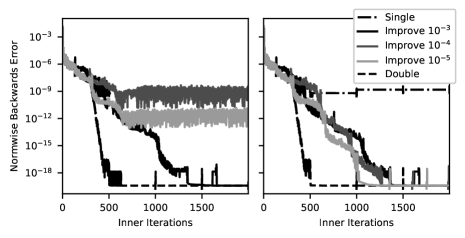
Figure 4: Rate of convergence results for the big matrix when restarting mixed-precision gmres after a fixed improvement in the Arnoldi residual norm for mgs (left) and cgsr (right) orthogonalization schemes, with vertical ticks to indicate when restarts occurred

Note that the successful threshold with the most improvement per restart is two orders of magnitude less improvement per restart than that of airfoil_2d. Next, Fig. 5 uses the first restart’s iteration count as the iteration limit for the subsequent restarts when solving the airfoil_2d system.

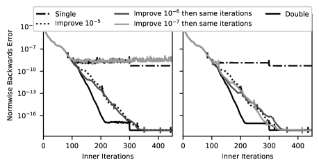
Figure 5: Rate of convergence results for the airfoil_2d matrix when restarting mixed-precision gmres after a fixed improvement in the Arnoldi residual norm for the first iteration and the same number of iterations thereafter for mgs (left) and cgsr (right) orthogonalization schemes, with vertical ticks to indicate when restarts occurred. The rate of convergence using just a fixed improvement threshold of $10^{-5}$ is added for comparison’s sake

Because only the choice of the first restart is important, a more ambitious threshold was chosen than for Fig. 3. Note that, except for when the first restart was not triggered, this two-staged approach generally performed a bit better than the simple threshold. Figure 6 shows the mixed restart strategy for the big matrix.

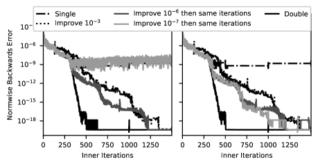
Figure 6: Rate of convergence results for the big matrix when restarting mixed-precision gmres after a fixed improvement in the Arnoldi residual norm for the first iteration and the same number of iterations thereafter for mgs (left) and cgsr (right) orthogonalization schemes, with vertical ticks to indicate when restarts occurred. The rate of convergence using just a fixed improvement threshold of $10^{-5}$ is added for comparison’s sake

Note how the same thresholds were used for the big test as the airfoil_2d test but were still able to converge and outperform the matrix-specific, scalar threshold. This two-part strategy appears to behave more consistently than the simple threshold.

Finally, we tested restarts based on the loss of orthogonality in the basis. Because cgsr retains a high degree of orthogonality, this strategy was only tested with mgs-gmres. Fig. 7 shows the rate of convergence when restarting based on the norm of the $S$ matrix.

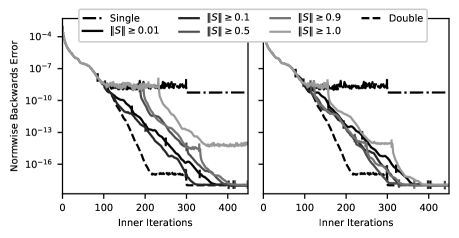
Figure 7: Rate of convergence results for the airfoil_2d matrix when restarting mixed-precision gmres based on the spectral norm (left) or Frobenius norm (right) of the $S$ matrix, for mgs orthogonalization, with vertical ticks to indicate when restarts occurred

The spectral norm was computed using 10 iterations of the power method. Additionally, the Frobenius norm was tested as a cheaper alternative to the spectral norm, although it does not provide the same theoretical guarantees. Interestingly, when using the spectral norm, a norm of even $0.5$ was not detected until improvement had stalled for a noticeable period. Note that even the Frobenius norm, which is an upper bound on the spectral norm, did not reach $1$ until, visually, improvement had stalled for a few dozen iterations. The cause of this deviation from the theoretical results [18] is unknown.

4.2 Performance

Finally, we looked at the effect of reduced precision on performance. Additionally, in testing a variety of matrices, these tests provide further support for some of the conclusions from Sec. 4.1. The runtimes include the time spent constructing the preconditioner and making any copies of the matrix. In addition to comparing the performance of mixed- and double-precision gmres, we tested the effect of reducing the precision of just the ILU preconditioner.

We first tested the performance improvement when other constraints force gmres to restart more often than required by mixed precision. For each of the tested systems, we computed the number of iterations for the double-precision solver to reach a backward error of $10^{-10}$. Then, we measured the runtime for each solver to reach a backward error of $10^{-10}$ when restarting after half as many iterations. All but 3 of the systems took the same number of iterations for mgs; two systems took fewer iterations for mixed precision (ecl32 and mc2depi), while one system took more iterations for mixed precision (dc1). cgsr added one additional system that took more iterations for mixed precision (big). Figure 8 shows the speedup of the mixed-precision implementation and the single-precision ILU implementation relative to the baseline implementation for each of the tested matrices.

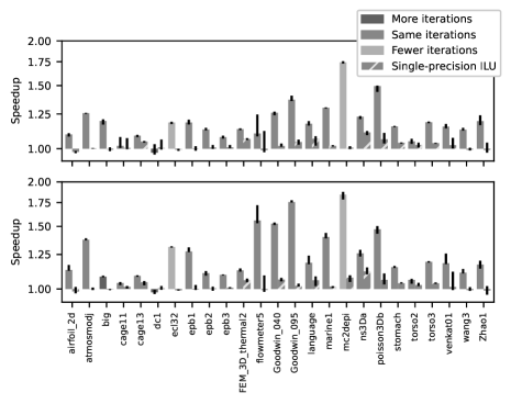
Figure 8: Speedup of the median runtime out of five tests for mixed-precision versus double-precision restarted in half the number of iterations needed for double-precision, for mgs (top) and cgsr (bottom) orthogonalization schemes, with error bars indicating the minimum and maximum speedups

For the mixed-precision implementation, the geometric mean of the speedup was 19% and 24% for mgs and cgsr, respectively. For the single-precision ILU implementation, those means were both 2%.

The second set of performance tests show what happens when gmres is not forced to restart often enough for mixed precision. All of the matrices from Fig. 8 that were restarted after fewer than 50 iterations were tested again, except they were restarted after 50 iterations. For mixed-precision gmres, the first restart could additionally be triggered by an improvement in the Arnoldi residual by a factor of $10^{-6}$ and subsequent restarts were triggered by reaching the number of inner-iterations that caused the first restart. To ensure the mixed-precision solver was not given any undue advantage, the other two solvers’ performance was taken as the best time from three restart strategies: (1) the same improvement-based restart trigger as mixed-precision gmres; (2) after 50 iterations, or (3) after an improvement in the Arnoldi residual by a factor of $10^{-8}$. Figure 9 shows the new performance results.

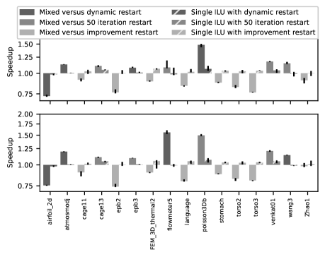
Figure 9: Speedup of the median runtime out of five tests for mixed-precision versus double-precision restarted after 50 iterations or an improvement in the Arnoldi residual, for mgs (top) and cgsr (bottom) orthogonalization schemes, with error bars indicating the minimum and maximum speedups

For the mixed-precision implementation, the geometric mean of the speedup was -4% and 0% for mgs and cgsr, respectively. For the single-precision ILU implementation, those means were 2% and 1% respectively. The matrices for which the mixed-precision implementation performed worse were exactly the matrices that did not require restarting when solved by the double-precision implementation.

5 Conclusion

As a widely used method for solving sparse, non-symmetric systems of linear equations, it is important to explore ways to improve the performance of gmres. Towards this end, we experimented with the use of mixed-precision techniques to reduce the amount of data moved across the cache hierarchy to improve performance. By viewing gmres as a variant of iterative refinement, we found that gmres was still able to achieve the accuracy of a double-precision solver while using our proposed techniques of mixed-precision and restart initiation. Furthermore, we found that the algorithm, with our proposed modifications, delivers improved performance when the baseline implementation already requires restarting for all but one problem, even compared to storing the preconditioner in single precision. However, our approach reduced performance when the baseline did not require restarting, at least for problems that require less than 50 inner iterations.

There are a few directions in which this work can be further extended. The first direction is to expand the implementation to a variety of systems that are different from a single CPU-only node. For example, GPU accelerators provide a significantly higher performance benefit than CPUs but involve a different trade-off between computational units, memory hierarchy, and kernel launch overheads. Thus, it would be beneficial to explore the use of mixed precision in gmres on these systems. Also important are the distributed memory, multi-node systems that are used to solve problems too large to be computed efficiently on a single node. In these solvers, the movement of data across the memory hierarchy becomes less important because of the additional cost of moving data between nodes. A related direction is to explore the use of mixed-precision techniques to improve variants of gmres. One particularly important class of variants is communication-avoiding and pipelined renditions for distributed systems, which use alternative formulations to reduce the amount of inter-node communication. The last major direction is to explore alternative techniques to reduce data movement. This can take many forms, including alternative floating-point representations, such as half-precision, quantization, or Posits [15]; alternative data organization, such as splitting the high- and low-order bytes of double-precision [14]; or applying data compression, such as SZ [16] or ZFP [17].

Acknowledgments

This material is based upon work supported by the University of Tennessee grant MSE E01-1315-038 as Interdisciplinary Seed funding and in part by UT Battelle subaward 4000123266. This material is also based upon work supported by the National Science Foundation under Grant No. 2004541.

References

- [1] Anzt, H., Heuveline, V., Rocker, B.: Mixed precision iterative refinement methods for linear systems: Convergence analysis based on Krylov subspace methods. In: Proceedings of the 10th International Conference on Applied Parallel and Scientific Computing - Volume 2, PARA’10, pp. 237–247. Springer-Verlag, Berlin, Heidelberg (2010). 10.1007/978-3-642-28145-7_24
- [2] Arnoldi, W.E.: The principle of minimized iteration in the solution of the matrix eigenvalue problem. Quart. Appl. Math. 9, 17–29 (1951). 10.1090/qam/42792
- [3] Baboulin, M., Buttari, A., Dongarra, J., Kurzak, J., Langou, J., Langou, J., Luszczek, P., Tomov, S.: Accelerating scientific computations with mixed precision algorithms. CoRR abs/0808.2794 (2008). 10.1016/j.cpc.2008.11.005
- [4] Baker, A.H.: On improving the performance of the linear solver restarted GMRES. Ph.D. thesis, University of Colorado (2003)
- [5] Baker, A.H., Jessup, E.R., Manteuffel, T.: A technique for accelerating the convergence of restarted GMRES. SIAM J. Matrix Anal. Appl. 26(962) (2005). 10.1137/S0895479803422014
- [6] Buttari, A., Dongarra, J., Langou, J., Langou, J., Luszczek, P., Kurzak, J.: Mixed precision iterative refinement techniques for the solution of dense linear systems. Int. J. High Perform. Comput. Appl. 21(4), 457–466 (2007). 10.1177/1094342007084026
- [7] Carson, E., Higham, N.J.: A new analysis of iterative refinement and its application to accurate solution of ill-conditioned sparse linear systems. SIAM J. Sci. Comput. 39(6), A2834–A2856 (2017). 10.1137/17M1122918
- [8] Davis, T.A., Hu, Y.: The University of Florida sparse matrix collection. ACM Trans. Math. Softw. 38(1) (2011). 10.1145/2049662.2049663
- [9] Edwards, H.C., Trott, C.R., Sunderland, D.: Kokkos: Enabling manycore performance portability through polymorphic memory access patterns. J. Parallel Distr. Comput. 74(12), 3202–3216 (2014). 10.1016/j.jpdc.2014.07.003
- [10] Giraud, L., Haidar, A., Watson, L.T.: Mixed-precision preconditioners in parallel domain decomposition solvers. In: U. Langer, M. Discacciati, D.E. Keyes, O.B. Widlund, W. Zulehner (eds.) Domain Decomposition Methods in Science and Engineering XVII, pp. 357–364. Springer Berlin Heidelberg, Berlin, Heidelberg (2008). 10.1007/978-3-540-75199-1_44
- [11] Giraud, L., Langou, J., Rozloznik, M.: The loss of orthogonality in the Gram-Schmidt orthogonalization process. Comput. Math. Appl. 50(7), 1069–1075 (2005). 10.1016/j.camwa.2005.08.009
- [12] Gratton, S., Simon, E., Titley-Peloquin, D., Toint, P.: Exploiting variable precision in GMRES. SIAM J. Sci. Comput. (to appear) (2020)
- [13] Greenbaum, A., Rozložník, M., Strakoš, Z.: Numerical behaviour of the Modified Gram-Schmidt GMRES implementation. Bit. Numer. Math. 37(3), 706–719 (1997). 10.1007/BF02510248
- [14] Grützmacher, T., Anzt, H.: A modular precision format for decoupling arithmetic format and storage format. In: Revised Selected Papers, pp. 434–443. Turin, Italy (2018). 10.1007/978-3-030-10549-5_34
- [15] Gustafson, J.L., Yonemoto, I.T.: Beating floating point at its own game: Posit arithmetic. Supercomput. Front. Innov. 4(2), 71–86–86 (2017). 10.14529/jsfi170206
- [16] Liang, X., Di, S., Tao, D., Li, S., Li, S., Guo, H., Chen, Z., Cappello, F.: Error-controlled lossy compression optimized for high compression ratios of scientific datasets. In: 2018 IEEE International Conference on Big Data (Big Data), pp. 438–447. IEEE (2018). 10.1109/BigData.2018.8622520
- [17] Lindstrom, P.: Fixed-rate compressed floating-point arrays. IEEE Trans. Vis. Comput. Graph. 20(12), 2674–2683 (2014). 10.1109/TVCG.2014.2346458
- [18] Paige, C.C.: A useful form of unitary matrix obtained from any sequence of unit 2-norm n-vectors. SIAM J. Matrix Anal. Appl. 31(2), 565–583 (2009). 10.1137/080725167
- [19] Paige, C.C., Rozlozník, M., Strakos, Z.: Modified Gram-Schmidt (MGS), least squares, and backward stability of MGS-GMRES. SIAM J. Matrix Anal. Appl. 28(1), 264–284 (2006). 10.1137/050630416
- [20] Paige, C.C., Strakos, Z.: Residual and backward error bounds in minimum residual Krylov subspace methods. SIAM J. Sci. Comput. 23(6), 1898–1923 (2001). 10.1137/S1064827500381239
- [21] Saad, Y.: Iterative Methods for Sparse Linear Systems, second edn. SIAM Press, Philadelphia, PA, USA (2003)
- [22] Saad, Y., Schultz, M.H.: GMRES: A generalized minimal residual algorithm for solving nonsymmetric linear systems. SIAM J. Sci. Stat. Comput. 7(3), 856–869 (1986). 10.1137/0907058
- [23] Van der Vorst, H.A., Vuik, C.: The superlinear convergence behaviour of GMRES. J. Comput. Appl. Math. 48(3), 327–341 (1993). 10.1016/0377-0427(93)90028-A
- [24] Wilkinson, J.H.: Rounding Errors in Algebraic Processes. Prentice-Hall, Princeton, NJ, USA (1963)