Spatiotemporal engineering of matter-wave solitons in Bose-Einstein condensates

Abstract

Since the realization of Bose-Einstein condensates (BECs) trapped in optical potentials, intensive experimental and theoretical investigations have been carried out for bright and dark matter-wave solitons, coherent structures, modulational instability (MI), and nonlinear excitation of BEC matter waves, making them objects of fundamental interest in the vast realm of nonlinear physics and soft condensed-matter physics. Many of these states have their counterparts in optics, as concerns the nonlinear propagation of localized and extended light modes in the spatial, temporal, and spatiotemporal domains. Ubiquitous models, which are relevant to the description of diverse nonlinear media in one, two, and three dimensions (1D, 2D, and 3D), are provided by the nonlinear Schrödinger (NLS), alias Gross-Pitaevskii (GP), equations. In many settings, nontrivial solitons and coherent structures, which do not exist or are unstable in free space, can be created and/or stabilized by means of various management techniques, which are represented by NLS and GP equations with coefficients in front of linear or nonlinear terms which are functions of time and/or coordinates. Well-known examples are dispersion management in nonlinear fiber optics, and nonlinearity management in 1D, 2D, and 3D BEC. Developing this direction of research in various settings, efficient schemes of the spatiotemporal modulation of coefficients in the NLS/GP equations have been designed to engineer desirable robust nonlinear modes. This direction and related ones are the main topic of the present review. In particular, a broad and important theme is the creation and control of 1D matter-wave solitons in BEC by means of combination of the temporal or spatial modulation of the nonlinearity strength (which may be imposed by means of the Feshbach resonance induced by variable magnetic fields) and a time-dependent trapping potential. An essential ramification of this topic is analytical and numerical analysis of MI of continuous-wave (constant-amplitude) states, and control of the nonlinear development of MI. Another physically important topic is stabilization of 2D solitons against the critical collapse, driven by the cubic self-attraction, with the help of temporarily periodic nonlinearity management, which makes the sign of the nonlinearity periodically flipping. In addition to that, the review also includes some topics that do not directly include spatiotemporal modulation, but address physically important phenomena which demonstrate similar soliton dynamics. These are soliton motion in binary BEC, three-component solitons in spinor BEC, and dynamics of two-component 1D solitons under the action of spin-orbit coupling.

Highlights

• A review is focused on 1D, 2D, and 3D matter-wave solitons in Bose-Einstein condensates under the action of spatiotemporally modulated cubic nonlinearity and time-dependent trapping potentials

• Most essential problems under the consideration is the shape and stability of solitons and other coherent structures, including stabilization against the critical collapse

• Both analytical results (exact and approximate ones) and systematically produced numerical findings are summarized

• The modulational instability in these models and its nonlinear development is addressed in detail

• Stability and motion of multi-component solitons in binary and spinor (triple) solitons is considered

Keywords Nonlinear Schrödinger equations; Gross-Pitaevskii equations; dispersion management; nonlinearity management; critical collapse; Feshbach-resonance technique; spin-orbit coupling; spinor Bose–Einstein condensate

Acronyms:

1D one-dimensional

2D two-dimensional

3D three-dimensional

BdG Bogoliubov - de Gennes (equations for small perturbations)

BEC Bose-Einstein condensate

CW continuous-wave (solution, alias plane wave)

DM dispersion management

FM ferromagnetic

FR Feshbach resonance

GP Gross-Pitaevskii (equation)

HO harmonic oscillator

MI modulational instability

NLS nonlinear Schrödinger (equation)

NM nonlinearity management

ODE ordinary differential equation

PIT phase-imprinting technique

SOC spin-orbit coupling

SPM self-phase-modulation (nonlinear self-interaction)

TS Townes’ soliton

VA variational approximation

XPM cross-phase-modulation (nonlinear interaction between two components)

I Introduction

The nonlinear Schrödinger (NLS) equations are basic models in a broad spectrum of disciplines in physics and engineering. Among these models, most thoroughly elaborated ones belong to the realms of nonlinear optics and Bose-Einstein condensates (BECs) of ultracold atoms. In this latter context, the NLS equation is often called the Gross-Pitaevskii (GP) equation. Commonly known fundamental solutions of the NLS equations are solitons (self-trapped localized states) Peyrard ; Yang . Many species of solitons have been predicted and observed in optics HK ; 0.1 and in BEC 3.30 ; Abdullaev ; Luca . In particular, many results have been produced in the framework of the dynamical management of solitons, under the action of time-dependent factors, which are represented by time-dependent terms in the respective NLS or GP equations 2.1 , that may also include linear losses and compensating gain. A well-known example is the dispersion management (DM) in fiber optics 2.1 ; Turitsyn , with the group-velocity-dispersion coefficient periodically alternating between positive and negative values along the propagation distance (which is the evolution variable in the guided-wave propagation theory HK ). This setting helps to stabilize DM solitons against various perturbations, such as random noise and collisions between solitons in multi-channel systems Nijhof ; coll1 ; coll2 ; 0.2 . Furthermore, the DM scheme was predicted to help stabilize 2D Michal and 3D Wagner spatiotemporal solitons (“light bullets”).

Another important variant of the NLS/GP models with the dynamical modulation include nonlinearity management (NM), i.e., a time-varying coefficient in front of the cubic term. This possibility was first elaborated in terms of the optics model, based on the two-dimensional (2D) spatial-domain NLS equation for the beam propagation in bulk media. Assuming that the medium was composed of alternating elements with self-focusing and defocusing Kerr (cubic) nonlinearity, it was demonstrated 4.7 that this version of NM stabilizes oscillating 2D solitons against the critical collapse (blowup), which makes all static 2D solitons (called Townes’ soliton (TS) Townes in this case) unstable in the uniform medium with the cubic self-focusing Fibich .

The concept of NM in optics, which ultimately aims to create nontrivial spatiotemporal light patterns, such as “bullets”, is naturally related to the rapidly developing area of experimental and theoretical studies aimed at the creation and various applications of structured light str-light0 ; str-light1 ; str-light3 ; str-light2 ; Forbes ; str-light-roadmap ; str-light-book . In most cases, the structure in light beams is induced by means of linear techniques (see, e.g., Ref. linear-shaping and references therein). Frequently, the so created light patterns take the form of a “flying focus”, with the focal point featuring controlled spatiotemporal motion flying-focus . Because nonlinearity is the underlying topic of the present article, it is relevant to mention that, very recently, a more powerful method was elaborated, which makes it possible to build optical fields with an embedded “self-flying-focus”, by means of inherent nonlinearity of the medium self-flying . Another experimentally implemented technique, which is very relevant in the context of models considered below in the present article, makes it possible to create arbitrarily structured averaged optical patterns “painted” by a rapidly moving laser beam paint .

In the GP equation, the cubic term accounts for effects of inter-atomic collisions in BEC, treated in the mean-field approximation, with the coefficient in front of it proportional to the s-wave collision scattering length Pit . In the experiment, this parameter can be controlled by means of the Feshbach-resonance (FR) effect, i.e., a change of the scattering length under the action of magnetic field, which creates short-lived quasi-bound states in the course of the inter-atomic collision Feshbach ; FR-review . It was demonstrated that the FR may be used to very accurately adjust the nonlinearity strength in BEC of potassium 4.15 and lithium 4.12 ; 0.7 atoms, as well as in binary BEC mixtures, such as one formed by ²³Na and ⁸⁷Rb atoms FR-mixture . The FR can also be imposed optically, by appropriate laser illumination FR-optical ; 0.5 ; 0.4 ; FR-Killian , as well as by microwave FR-micro and electrostatic FR-electro fields. Then, NM for BEC may be realized using time-dependent and/or nonuniform control fields 2.1 ; 0.1 ; 0.3 ; 0.4 ; 0.5 ; Pelster ; Barcelona ; 05feb . In particular, the FR technique makes it possible to quickly reverse (in time) the interaction sign from repulsion to attraction (positive to negative scattering length), which gives rise, via the onset of the collapse, to abrupt shrinkage of the condensate, followed by a burst of emitted atoms and the formation of a stable residual condensate Weiman . A similar method relies on the use of quench, i.e., sudden change of the self-attraction strength in BEC, which makes it possible to transform a quasi-1D fundamental soliton into an oscillatory state in the form of a breather breather . A still more spectacular outcome is “bosonic fireworks” in the form of violent emission of matter-wave jets from the original condensate fireworks1 ; fireworks2 . In other experiments, the time-periodic modulation of the nonlinearity strength, applied to the quasi-1D (cigar-shaped) BEC, initiates a transition to a granulated state in the condensate granulation .

In the case of the attractive interaction, matter-wave solitons may be readily formed in an effectively 1D condensate 3.30 . However, in the 2D geometry the attraction results in the critical collapse of the condensate, if the number of atoms (the norm of the wave field, in terms of the GP equation) exceeds a critical value. The FR technique was predicted to be quite useful in these settings: similar to the above-mentioned results for the 2D spatial solitons in the optical bulk waveguide with the periodic alternation of the self-focusing and defocusing 4.7 , 2D matter-wave solitons may be readily stabilized against the critical collapse by the time-periodic variation of the nonlinearity coefficient between negative and positive values. This approach was elaborated in detail in various forms 3.1 ; Ueda ; VPG ; Itin . Unlike the fundamental 2D solitons, the NM scheme cannot stabilize 2D solitons with embedded vorticity against the splitting instability (to which the vortex solitons are most vulnerable PhysicaD ), and it cannot stabilize 3D solitons against the supercritical collapse either (in the latter case, the critical norm is zero, i.e., any value of the norm may lead to the collapse). However, 3D solitons can be stabilized if the NM is combined with a quasi-1D spatially periodic potential (optical lattice) applied to the condensate Michal2 . A generalization of the FR technique for controlling the strength and sign of the interaction between atoms in BEC and, thus, the coefficient in front of the cubic term in the corresponding GP equation, is the application of a control field containing time-periodic (ac) and constant (dc) components. Another essential ramification is the use of FR in BEC mixtures, to adjust the relation between strengths of self- and cross-component interactions (alias self- and cross-phase modulation, SPM and XPM, in terms of nonlinear optics 0.1 ), which helps to produce robust multi-component states in the experiment 0.6 ; Dimitri ; mixed-droplet .

A natural generalization of the NM scenarios for BEC is to combine the variable coefficient in front of the nonlinear term in the GP equation, imposed by the temporal and/or spatial modulation of the scattering length, with a temporarily modulated potential trapping the condensate. In particular, a specially designed relation between the spatiotemporal dependence of nonlinear and linear factors in the GP equation makes it possible to produce integrable versions of the equation in 1D WMLiu-PRL ; Zhong ; Zhong4 ; 2.7 ; Lakshmanan ; LuLi ; WMLiu ; Cardoso ; add8 . A similar approach was developed for constructing solvable 3D models, which admit factorization of the respective 3D equation into a product of relatively simple 1D equations, which admit exact solutions (in particular, solitons) Zhong2 ; Zhong3 ; Belic ; Zhong3D ; Zhong3D-2 . In fact, the integrability of such specially designed (engineered) models is not a fundamentally new mathematical finding, because they may be transformed, by means of tricky but explicit transformations of the wave function (or several wave functions, in the case of multi-component systems), spatial coordinates, and the temporal variable, into the classical integrable 1D NLS equation with constant coefficients (or the Manakov’s 4.14 integrable system of the NLS equations) Suslov ; cubic-quartic . Accordingly, a great variety of integrable and nearly integrable models can be generated by means of inverse engineering, applying generic transformations of the same type to the underlying integrable equation(s) Stepa . Although this approach to the expansion of the set of solvable models seems somewhat artificial, it is meaningful, and quite useful in many cases, as it has a potential to predict tractable nontrivial configurations in BEC and, to a lesser degree, in optics (it is not easy to apply flexible modulation of local nonlinearity to optical media, where there is no direct counterpart of FR).

In this review article, we summarize basic results (chiefly, theoretical ones) for the dynamics of BEC and optical fields trapped in time-dependent potentials, combined with the variable (time-modulated) nonlinearity. The respective models are based on one-, two-, and three-component nonautonomous GP/NLS equations. It is relevant to stress that all the results included in the review have already been published, although some of them are quite recent. In particular, an essential direction in these studies, elaborated in many theoretical works, is the design of specific nontrivial models which can be explicitly transformed into an integrable form, thus making it possible to use the huge stock of exact solutions, available in the original models. The analytically found exact solutions are, in many cases, confirmed by numerical simulations. It is necessary to stress that, while the exact solutions are stable in the framework of the integrable models, they may be subject to the structural instability, as a small deviation of the physical model from the integrable form may lead to the loss of stability of the original exact solutions, or even make them nonexistent, in the rigorous mathematical sense. In such cases, the former solutions will suffer slow decay; however, it may often happen that the decay time (or propagation distance, in optics) will be essentially larger than the actual extension of plausible experiments, hence the approximate solutions still predict physically relevant states.

The rest of the article is composed of sections which are related by gradually increasing complexity of models presented in them. Section 2 addresses the basic model, in which the approach outlined above leads to the construction and management of nonautonomous solitons of 1D cubic self-defocusing NLS equations with spatiotemporally modulated coefficients, that may be transformed into the classical integrable NLS equation. In this setting, matter-wave soliton solutions are constructed in an analytical form, and it is shown that the instability of those solitons, if any, may be delayed or completely eliminated by varying the nonlinearity’s strength in time. In Section 3, we continue the presentation by considering engineered nonautonomous matter-wave solitons in BEC with spatially modulated local nonlinearity and a time-dependent harmonic-oscillator (HO) potential. The modulational instability (MI) in that setting is considered too. In Section 4, we proceed to more general nonintegrable models, which are treated by means of the semi-analytical variational approximation (VA) and direct numerical simulations. In this case, we address the dynamics of 2D and 3D condensates with the nonlinearity strength containing constant and harmonically varying parts, which can be implemented with the help of ac magnetic field tuned to FR. In particular, the spatially uniform temporal modulation of the nonlinearity may readily play the role of an effective trap that confines the condensate, and sometimes enforces its collapse. Section 5 deals with dynamics of a binary (two-component) condensate in an expulsive time-varying HO potential with the time-varying attractive interaction. In this case, the condensates in the expulsive time-modulated HO potential may sustain the stability, while their counterparts in the time-independent potential rapidly decay. In Section 6, we address the dynamics of matter-wave solitons of coupled GP equations for binary BEC. Strictly speaking, this model does not include spatiotemporal engineering of solitons, but the results are closely related to those produced by means of the engineering. In particular, the results reported in section 6 show that, in the absence of the XPM interaction, the solutions maintain properties of one-component condensates, such as MI, while in the presence of the interaction between the components, the solutions exhibit different properties, such as restriction of MI and soliton splitting. Section 7 deals with the soliton states in a model based on a set of three coupled GP equations modeling the dynamics of the spinor BEC, with atomic spin $F=1$. Both nonintegrable and integrable versions of the system are considered, and exact soliton solutions are demonstrated. The stability of the solutions was checked, in most cases, by direct simulations and, in some cases, it was investigated in a more rigorous form, based on linearized Bogoliubov - de Gennes (BdG) equations for small perturbations. In Section 8, we introduce a new physical setting, considering the motion of bright and dark matter-wave solitons in 1D BEC in the presence of spin-orbit coupling (SOC). We demonstrate that the spin dynamics of the SOC solitons is governed by a nonlinear Bloch equation and affects the orbital motion of the solitons, leading to SOC effects in the dynamics of macroscopic quantum objects. Similar to what is mentioned about Section 6, the settings addressed in Sections 7 and 8 do not directly include ingredients of the spatiotemporal engineering. Nevertheless, the models addressed in these sections, as well as methods applied to them and obtained results, are quite similar to those produced by the engineering. In particular, the macroscopic SOC phenomenology is explained by the fact that an effective time-periodic force produced by rotation of the soliton’s (pseudo-) spin plays the role of temporal management which affects motion of the same soliton. Each Section 2 through 8 contains formulation of the underlying model, summary of analytical and numerical results, and a conclusion focused in the topic under the consideration, with references to original papers in which those results have been reported. Finally, Section 9 concludes the review and mentions perspectives for further work in this area.

The presentation has a rather technical form, as the topic surveyed in this article is inherently technical. Nevertheless, an effort is made, in each section, to highlight the main findings, on top of technical details. The sections include an outline of physical realizations of the considered theoretical models in BEC (and in some cases, in nonlinear optics). Characteristic physical parameters of the respective settings, such as atomic species and particular atomic states, relevant numbers of atoms, the scattering and transverse-confinement lengths, etc., are given too.

II Management of matter-wave solitons in BEC with time modulation of the scattering length and trapping potential

The present section deals with nonautonomous solitons produced by 1D self-defocusing GP equations with the nonlinearity coefficient subject to spatiotemporal modulation and a time-dependent trapping potential. The respective model is the basic one in the framework of the topic considered in this review. We start by presenting stable higher-order modes in the form of arrays of dark solitons nested in a finite-width background. Then, we show that the dynamics of those modes from this class which are not stable can be efficiently controlled (attenuated or completely suppressed) by varying the nonlinearity strength in time.

Results collected in this section are based on original works 2.12 ; 2.13 ; 2.6 ; 2.7 and 2.5a .

II.1 The model and stationary solitons

II.1.1 Formulation of the model

The setting addressed in this section is based on the 1D NLS/GP equation, written in the normalized form:

$$i\frac{\partial\psi}{\partial\xi}=-\frac{\partial^{2}\psi}{\partial x^{2}}+g(\xi,x)\left|\psi\right|^{2}\psi+V(\xi,x)\psi,$$ (1)

where $\psi$ is the mean-field wave function of the quasi-1D (cigar-shaped) BEC if $\xi$ stands for time, $x$ is the axial coordinate, $V\left(\xi,x\right)$ the time-dependent axial potential, and the strength of the cubic nonlinearity, $g$, is proportional to the interatomic s-wave scattering length. The effective 1D equation is derived from the full 3D GP equation if the cigar-shaped configuration is confined, in transverse plane $\left(y,z\right)$, by the strong transverse HO potential with frequency $\omega_{\perp}$ and the respective confinement radius $a_{\perp}=\sqrt{\hslash/(m\omega_{\bot})}$, where $m$ is the atomic mass. To this end, the 3D mean-field wave function is approximately factorized into the product of its axial (1D) counterpart, in which time $\xi$ and coordinate $x$ are measured in units of $2/\omega_{\bot}$ and $a_{\bot}$, and the HO ground-state wave function in the transverse plane Salasnich :

$$\Psi(\mathbf{r},\xi)=\frac{1}{\sqrt{2\pi a_{\mathrm{B}}a_{\bot}}}\exp\left(-i\omega_{\bot}\xi-\frac{y^{2}+z^{2}}{2a_{\bot}^{2}}\right)\psi\left(\omega_{\bot}\xi,\frac{x}{a_{\bot}}\right),$$ (2)

where $a_{\mathrm{B}}$ is the Bohr radius. It is relevant to mention that, for very dense BEC, the 3D $\rightarrow$ 1D dimension reduction may lead to more complex effective 1D equations, with nonpolynomial nonlinearities Salasnich ; Delgado . Another caveat is that the reduction to the 1D GP equation is relevant for $a_{\perp}$ taking values in the $\mathrm{\mu}$m range, which is the usual experimental situation. If the transverse-confinement radius is reduced much deeper, to make it comparable to the effective atomic size, the quasi-1D BEC transforms into a different quantum state, viz., the Tonks-Girardeau gas TG .

As outlined above, the spatiotemporal modulation may be imposed on the nonlinearity coefficient $g(\xi,x)$ by the FR technique, controlled by variable magnetic field 2.1 ; 2.2 ; Zhang ; granulation or by an appropriately shaped optical field submicroOL . Positive and negative values of $g$ correspond, respectively, to the repulsive (alias self-defocusing) and attractive (focusing) contact interactions. In the latter case, the nonlinear self-attraction drives the onset of MI in the condensate 2.3 ; RandyMI ; CanberraMI . Note that the spatiotemporal modulation may create a sign-changing pattern of $g$, with alternating self-focusing and defocusing regions Barcelona .

If $\xi\$is the propagation distance, Eq. (1) governs the propagation of an optical beam in a planar waveguide along the $\xi$ direction, the external potential being, in this case, generated by a modulation of the local refractive index 2.4 , while various forms of $g(\xi,x)$ may be realized by means of accordingly designed distributions of nonlinearity-enhancing dopants 2.5 .

II.1.2 Stationary soliton states for $V=V(x)$ and $g=g(x)$:

First, we address stationary solutions of Eq. (1) with both $g$ and $V$ being functions of coordinate $x$ only. Obviously, in the general case the respective stationary GP equation is not analytically solvable in the general form. However, there is a method to select specific forms of $g(x)$ and $V(x)$ which admit exact solutions 2.6 ; 2.7 ; 2.5a . To this end, full soliton solutions to Eq. (1) were looked for in Ref. 2.5a as

$$\psi(\xi,x)=\rho(x)u(X)\exp\left(-i\mu\xi\right),$$ (3)

where $\mu$ is a real chemical potential (in the application to optics, $-\mu$ is the propagation constant). Further, a new coordinate is identified as

$$X(x)\equiv\int_{-\infty}^{x}ds/\rho^{2}(s),$$ (4)

with real function

$$\rho(x)=\sqrt{\alpha\varphi_{1}^{2}+2\beta\varphi_{1}\varphi_{2}+\gamma\varphi_{2}^{2}},$$ (5)

where $\varphi_{1,2}(x)$ are two linearly independent solutions of the ordinary differential equation (ODE)

$$d^{2}\varphi/dx^{2}+\left[\mu-V(x)\right]\varphi=0,$$ (6)

$\alpha,\beta>0$ and $\gamma$ being real constants satisfying constraint

$$\alpha\gamma-\beta^{2}>0$$ (7)

(these conditions imply that $\rho(x)$ remains real and never vanishes). Inserting expression (3) under conditions (5) and (6) and defining the nonlinearity coefficient as

$$g(x)=\frac{F(u)}{\rho^{6}(x)},$$ (8)

where $F(u)$ is another real function, leads to ODE

$$Eu=\frac{d^{2}u}{dX^{2}}+F(u)u^{3}\text{, \ \ }E=\left(\alpha\gamma-\beta^{2}\right)W^{2},$$ (9)

where $W=W\left[\varphi_{1},\varphi_{2}\right]=\varphi_{1}d\varphi_{2}/dx-\varphi_{2}d\varphi_{1}/dx$ is the constant Wronskian of the pair of solutions $\varphi_{1,2}(x)$. Because condition (7) guarantees that $\rho(x)$ does not vanish at all $x$, the coefficient function $g$ defined by Eq. (8) does not have singularities. Moreover, condition (7) also secures $E>0$ in Eq. (9).

Finally, looking for exact soliton solutions to the underlying equation (1) in the form given by Eqs. (3)-(5) amounts to finding exact solutions of ODE (9), which may be obtained with various choices of function $F(u)$. As it follows from Eq. (8), $F(u)$ is positive or negative in the whole spatial domain for the NLS equation whose nonlinearity is, respectively, defocusing (positive) or focusing (negative). In particular, the choice of $F(u)=g_{3}+g_{5}u^{2}$, casts Eq. (9) into the following solvable cubic-quintic ODE: $d^{2}u/dX^{2}+g_{3}u^{3}+g_{5}u^{5}+\left(\beta^{2}-\alpha\gamma\right)W^{2}u=0,$ where the cubic and quintic coefficients $g_{3}$ and $g_{5}$ with opposite signs, $g_{3}g_{5}<0$, correspond to the competing nonlinearities.

In what follows, we consider exact solutions of Eq. (9) for a more sophisticated choice,

$$F(u)=\frac{Eu-\sin\left[Eu\right]}{u^{3}},$$ (10)

which makes Eq. (9) tantamount to the stationary sine-Gordon equation, $d^{2}u/dX^{2}+\sin\left(Eu\right)=0$ 2.5a . Under condition $E>0$, it represents motion of a pendulum, i.e., either oscillations, with $u$ being a periodic function of $X$, or the rotation, with $U$ linearly growing, on the average. Relevant solutions of Eq. (1) correspond to periodic solutions for $u(X)$. Thus, one takes

$$u(X)=\frac{2}{E}\arcsin\left[q~{}\mathrm{sn}\left(\sqrt{E}X,q\right)\right],$$ (11)

where $\mathrm{sn}$ is the Jacobi’s elliptic sine with modulus $q$, the respective period of $u(X)$, as given by Eq. (11), being $4K(q)/\sqrt{E}$, where $K(q)$ is the complete elliptic integral of the first kind.

Inserting expressions (10) and (11) in Eq. (8), one finds that the nonlinearity coefficient supporting this exact solution has the defocusing sign, i.e., $g(x)>0$. Further, an external axial potential $V(x)$ is needed to confine the solution. The most physically relevant confining potential is the HO one, $V(x)=\omega_{0}x^{2}$. In this case, solutions $\varphi_{1}(x)$ and $\varphi_{2}(x)$ of ODE (6) can be expressed in terms of the Whittaker and Watson functions $M$ and $W$ 2.8 , and the Gamma function, $\Gamma$, as follows:

$$\varphi_{1}(x)=\frac{\text{{sign}}\left(x\right)}{\omega_{0}^{3/4}\sqrt{\left|x\right|}}M(x)\text{, \ \ }$$

$$\varphi_{2}(x)=\frac{1}{\sqrt[4]{\omega_{0}}\sqrt{\pi\left|x\right|}}\left[\Gamma\left(\frac{3\omega_{0}-\mu}{4\omega_{0}}\right)W(x)+2\sqrt{\pi}M(x)\right],$$ (12)

provided that

$$\mu\neq\widetilde{\mu}^{(\ell)}\equiv\left(2\ell+1\right)\omega_{0},\ell=0,1,2,\cdots,$$ (13)

with $\widetilde{\mu}^{(\ell)}$ being the $\ell$-th HO energy eigenvalue. Because $\varphi_{1}(0)=d\varphi_{2}/dx|_{x=0}=0$ and $d\varphi_{1}/dx|_{x=0}=\varphi_{2}(0)=1$, the respective Wronskian is $W=-1$.

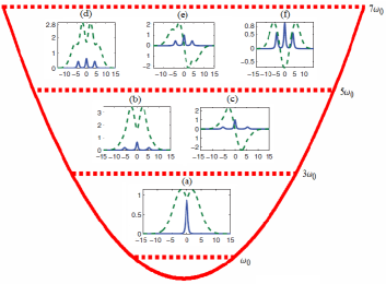
Figure 1: (Color online) The relation between the number of exact soliton solutions of Eq. (1), given by Eqs. (3), (4), (5), (8), and (11), and the discrete energy levels of the harmonic-oscillator potential (the underlying parabola). (a) Modulation profiles of the defocusing nonlinearity $g(x)$ (the solid line), and the shape of the exact soliton (the dashed line), for $\mu=0.2$, $n=1$, and $q=0.7458$. The horizontal axis is coordinate $x$. Other plots display the same for (b) $\mu=0.4$, $n=1$, $q=0.9984$, (c) $\mu=0.4$, $n=2$, $q=0.8586$, (d) $\mu=0.6$, $n=1$, $q=0.9998$, (e) $\mu=0.6$, $n=2$, $q=0.9530$, and (f) $\mu=0.6$, $n=3,$ $q=0.5933$. Other parameters are $\alpha=\sqrt[3]{6}$, $\beta=0$, $\gamma=1$, and $\omega_{0}=0.1$. Source: Reproduced from Ref. 2.5a .

Here we focus on the basic case of symmetric profiles of the nonlinearity modulation and the corresponding solitons by setting $\beta=0$ in Eq. (5). To produce a typical example, one can set $\omega_{0}=0.1$, $\alpha=6^{1/3}$, and $\gamma=1$, which makes $g(x)\sim 1$ close to the midpoint, $x=0$. Then, for given $\mu$, $\rho(x)$ and $X(x)$ can be calculated. To meet the zero boundary conditions at $x=\pm\infty$, which implies the localization of the solution, elliptic modulus $q$ must satisfy a constraint, $2nK(q)=\sqrt{E}R$, where $n$ is a positive integer and $R\equiv\int_{-\infty}^{+\infty}ds/\rho^{2}(s)$. It follows from condition $K(q)>\pi/2$ that $n$ is bounded from above, $n<\sqrt{E}R/\pi$, hence there is only a finite number of the exact solutions for given $\mu$. Integer $n$ is the order of the soliton mode, which features $n-1$ density nodes. Further analysis demonstrates that $\sqrt{E}R/\pi$ increases monotonically as $\mu$ increases, while other parameters are fixed, and $n$ takes values up to $\ell+1$ when $\widetilde{\mu}^{(\ell)}<\mu<\widetilde{\mu}^{(\ell+1)}$ (see Eq. (13)), there being no solutions at $\mu<\widetilde{\mu}^{(0)}$, see Fig. 1. An explanation for this result is that the defocusing nonlinearity pushes the energy levels up relative to the HO spectrum. Thus, the fundamental solitons ($n=1$) exist at $\mu>\widetilde{\mu}^{(0)}$, first-order excited solitons ($n=2$) exist at $\mu>\widetilde{\mu}^{(1)}$, and so on. This conclusion coincides with findings reported in Ref. 2.9 for the spatially homogeneous defocusing nonlinearity. A similar result holds for gap solitons in self-defocusing media: only first $n$ families of the solitons exist when $\mu$ lies in the $n$-$\mathrm{th}$ optical-lattice-induced bandgap 2.10 .

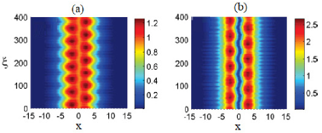
Figure 2: (Color online) (a) Oscillations of the soliton from Fig. 1(a) which was left-kicked with velocity $0.1$, the corresponding initial condition for Eq. (1) being $\rho(x)u[X(x)]\exp\left(-0.05ix\right)$. (b) Oscillations of the soliton from Fig. 1(c), which was left-kicked with initial velocity $0.05$. Reproduced from Ref. 2.5a .

In accordance with the above analysis, we show in Fig. 1(a) that only one exact soliton exists when $\mu=0.2$. The corresponding single-humped nonlinearity-modulation profile is localized near $x=0$, and the exact soliton has a small dip, because of the self-repulsive sign of the nonlinearity. Stability of the exact soliton solutions was checked by means of direct simulations of the perturbed evolution in the framework of Eq. (1). In particular, if kicked with initial velocity $0.1$, the soliton remains stable, featuring periodic oscillations in the trapping, as shown in Fig. 2(a).

Figure 3: (Color online) (a) The profile of the spatially modulated nonlinearity and (b) unstable evolution of the soliton from Fig. 1(e). (c) The spatiotemporal nonlinearity modulation and (d) the unstable evolution of the soliton, for the same initial conditions as in panel (b), but with the nonlinearity taken as per Eq. (18), and with half the trapping frequency, $\omega=\omega_{0}/2$. Reproduced from Ref. 2.5a .

With the help of the numerical integration in imaginary time, it was found that the fundamental soliton in the present model represents the ground state, which explains its robustness. As the solution parameter $\mu$ increases, more and more exact solitons appear, while the nonlinearity profile develops several peaks. In particular, it is seen from Figs. 1(b) and 1(c) that two exact solitons exist in the case of $\mu=0.4$. Figure 2(b) demonstrates that, besides the fundamental soliton, the first excited-state solution, which looks like a dark soliton nested in a finite-width background, is also stable. However, for $\mu=0.6$, the exact first and second excited-state solitons are unstable, see Fig. 3(b) for the former one. While it was not easy to analyze the stability of all the solitons corresponding to the excited states, it was possible for larger values of $\mu$ to generate arrays of nested dark solitons which maintain their stability—in particular, if small spatially homogeneous (Fig. 4(b)) or inhomogeneous (Fig. 4(c)) kicks are applied to them. This finding suggests a new approach to constructing soliton chains in the form of the Newton’s cradle cradle , and creating supersolitons, i.e., robust localized excitations running through a soliton chain supersol in systems described by the scalar NLS equation. In BEC trapped in a shallow HO potential, chains of dark solitons supporting the propagation of supersoliton modes, can be readily generated in the experiment by means of the phase-imprinting technique (PIT) imprint ; 2.11 ; 2.5a ; Hamburg .

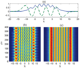
Figure 4: (Color online) (a) The modulation profile of the defocusing nonlinearity and the corresponding exact soliton (solid and dashed lines, respectively) for $\mu=1.6$, $n=8$, and $q=0.4752$. (b,c) The quasi-stable evolution of the soliton. The input for Eq. (1), used to generate panel (b), is $\rho(x)u[X(x)]\exp\left(-0.05ix\right)$, while panel (c) was created by input $\rho(x)u[X(x)]\exp\left(-0.05i\left|x\right|\right)$. Reproduced from Ref. 2.5a

Note that, for a fixed chemical potential $\mu$, there is one-to-one correspondence between the exact solution and nonlinearity profile $g(x)$. On the other hand, for fixed $g(x)$, one can always find other numerical soliton solutions, by varying $\mu$ and using the relaxation method. It was checked that, if the exact soliton is stable, its counterparts numerically found for the same spatially modulated nonlinearity coefficient $g(x)$ are also stable, provided that the chemical potential $\mu$ does not vary too much 2.5a . Further, it was checked that the numerically constructed solitons remain stable too when the nonlinearity profiles were taken somewhat different from the special form defined by (8). Therefore, higher-order solitons are physically meaningful objects.

II.2 Stability control of nonautonomous solitons

Next, following Ref. 2.12 , we address the model based on Eq. (1) in which $V$ and $g$ are functions of both $\xi$ and $x$. With specially designed coefficient functions $g(\xi,x)$ and $V\left(\xi,x\right)$, exact soliton solutions can be constructed by dint of a self-similar transformation which reduces the original equation to the standard integrable NLS equation 2.13 . The transformation is introduced as

$$\psi(\xi,x)=\frac{1}{\sqrt{w(\xi)}}\Phi(T,Y)\exp\left(-\frac{1}{4w}\frac{dw}{d\xi}x^{2}\right),$$ (14)

where

$$T\equiv\int_{0}^{\xi}ds/w^{2}(s),~{}Y\equiv x/w(\xi).$$ (15)

Inserting expression (14) in Eq. (1) and choosing $w$ as a solution of ODE

$$\frac{d^{2}w}{d\xi^{2}}+4\omega(\xi)w-4\frac{\omega_{0}^{2}}{w^{3}(\xi)}=0$$ (16)

yields

$$i\frac{\partial\Phi}{\partial T}=-\frac{\partial^{2}\Phi}{\partial Y^{2}}+\omega_{0}^{2}Y^{2}\Phi+g_{2}(Y)\left|\Phi\right|^{2}\Phi,$$ (17)

if the cubic nonlinearity parameter $g$ and external potential $V$ are chosen as

$$g(\xi,x)=g_{1}(\xi)g_{2}(Y),\text{ \ \ }V(\xi,x)=\omega(\xi)x^{2},\text{ \ with }g_{1}(\xi)=1/w(\xi)\text{.}$$ (18)

As seen from Eq. (18), $w(\xi)$ is the width of the nonlinearity modulation, and determines the soliton’s width.

To produce exact solutions of Eq. (17), the exact stationary soliton solutions displayed in Fig. 1 are used, replacing $Y$ by $x$, $g_{2}$ by $g$, $T$ by $\xi$ , and $\Phi$ by $\psi$. Moreover, given the functional form of $\omega(\xi)$, such as, e.g., $a_{0}+a_{1}\cos\xi$, equation (16) for $w(\xi)$ can be solved. Then, one can construct exact nonstationary soliton solutions of Eq. (1) as per Eq. (14).

The stability of the nonstationary solitons is related to that of the corresponding stationary solution and the functional form of $w(\xi)$. If the stationary soliton of Eq. (17) is stable, the respective nonstationary soliton of Eq. (1), produced by the transformation of the stable stationary one, is stable too. However, if the stationary soliton is unstable, with the instability setting in, say, at $T=T_{0}$, the instability of the nonstationary soliton may be delayed or even suppressed, choosing an appropriate form of $w(\xi)$. Namely, if $T$, defined as per Eq. (15), remains smaller than $T_{0}$, the instability is completely prevented, because the system does not have enough time (propagation distance) to reach the instability threshold. Otherwise, the onset of the instability is delayed.

As a typical example, we display the exact soliton corresponding to Fig. 1(e). Without the temporal nonlinearity modulation, its instability starts at $\xi\approx 40$ [see Fig. 3(b)]. If, at $\xi=0$, the trapping frequency is abruptly reduced by half, and after that the nonlinearity is varied as per Eq. (18) with $w(\xi)=\sqrt{1+3\sin^{2}\left(\omega_{0}\xi\right)}$ (see Fig. 3(c)), one finds that the soliton first experiences exact self-similar evolution in accordance with Eq. (14), and then it starts to develop instability at $\xi\approx 81$, determined by condition $40=\int_{0}^{\xi}ds/w^{2}(s)$, see Fig. 3(d). Clearly, the instability onset is delayed. It can be delayed further if one decreases the trapping frequency more, varying the nonlinearity accordingly. It is also relevant to mention that self-similar dynamical regimes find other important realizations in the mean-field dynamics, such as the collapse (blowup) regime self-sim ; Fibich .

II.3 Conclusion of the section

The subject of the section is to demonstrate well-known results which play the basic role in the topic of the present review, as they are produced by the basic model. These results produce exact soliton solutions to the NLS equation with the coefficient in front of the cubic nonlinearity and external potential subject to specially designed spatiotemporally modulation, that allows one to explicitly transform the equation into the classical integrable NLS equation. The number of solitons is determined by the value of the chemical potential and discrete energy levels of the trapping HO potential. The existence of stable higher-order modes, built as arrays of dark solitons embedded in the finite-width background, is demonstrated too. Finally, it is shown how one can control instability of nonstationary solitons, by choosing the temporal modulation which delays or completely eliminates the onset of the instability.

III Engineering nonautonomous solitons in Bose-Einstein condensates with a spatially modulated scattering length

As a characteristic example of BEC models with a spatially modulated scattering length, diverse versions of which have been theoretically elaborated in many works, see a review in Ref. Barcelona , we here consider, first, the corresponding cubic GP equation, and then the application of PIT to obtain a nonautonomous cubic derivative NLS equation, which includes a time-dependent HO potential. PIT is a relatively new tool used for wave-function engineering in BEC. It may be extended to control the wave function by means of absorption provided by proximity to a resonance with frequencies of external laser illumination. The action of PIT onto BEC amounts to modifying the phase pattern in the mean-field wave function—for example, by exposing the condensate to the action of pulsed, off-resonant laser light with a specially designed intensity pattern. As a result, atoms experience the action of a spatially varying light-induced potential, and thus acquire the corresponding phase. The main advantage of the application of PIT for BECs is that it conserves the total number of atoms.

Results collected in this section are based on original works 3.39 , 3.35 , 3.33 , and 3.33b . Some methods presented in the section refer to a recently published book 3.5 .

III.1 Introduction to the section

In the derivative NLS equation with the spatiotemporal modulation of the contact nonlinear term and time-variable potential,

$$i\,\frac{\partial\phi(x,t)}{\partial t}+\left[\frac{\partial^{2}}{\partial x^{2}}+\widetilde{g}(x,t)\left|\phi(x,t)\right|^{2}+\widetilde{V}(x,t)\right]\phi(x,t)+i\widetilde{\beta}\frac{\partial\left(|\phi|^{2}\phi\right)}{\partial x}=0,$$ (19)

the derivative cubic term represents the delayed nonlinear response of the system. Well-known in plasma physics, Eq. (19) models the propagation of finite-amplitude Alfvén waves in directions nearly parallel to the external magnetic field in a plasma with the gas pressure much smaller than the magnetic pressure (low-$\beta$ plasma) 3.26 . Other physical realizations of the derivative NLS equation are provided by convection in binary fluids 3.34 and propagation of signals in electric transmission lines 3.35 . Furthermore, an equation of type (19) governs the behavior of large-amplitude magnetohydrodynamic waves propagating in an arbitrary direction with respect to the magnetic field in high-$\beta$ plasmas 3.27 , see also review Kamchatnov . In nonlinear optics, the propagation equation for very short pulses the local Kerr nonlinearity has to be supplemented by the derivative self-steepening term, which accounts for the nonlinear dispersion of the optical material 3.28 ; 4.2 ; YangShen ; 6.3 . If $\widetilde{g}=\mathrm{const}$ and the external potential is absent, i.e., $\widetilde{V}=0$, Eq. (19) reduces to the-well known integrable derivative cubic NLS equation, which can be derived from the usual NLS equation by means of the $U(1)$ gauge transformation KaupNewell ; 3.29 . Two basic questions arise, as concerns equations of this type, in the context of this review: (i) How should one introduce a GP model describing the impact of the cubic derivative nonlinearity on the condensates? (ii) How does the derivative cubic term in the GP equation affect the MI in BEC? The main aim of the present section is to address these questions. To this end, we first demonstrate derivation of the extended NLS equation of type (19), in the case when PIT 3.33 ; 3.33b is applied to the setting modeled by GP equation with the spatiotemporally modulated contact–nonlinearity coefficient and time-dependent HO trapping potential.

III.2 The cubic inhomogeneous NLS equation

As mentioned above, FRs may be widely used to control the nonlinearity of matter waves, by modulating the scattering length of inter-atomic collisions temporarily, spatially, or spatiotemporally, which leads to generation of many novel nonlinear phenomena 3.30 ; 3.31 ; 3.32 . In particular, as outlined in the Introduction, it has been predicted that time-dependent modulation of the scattering length can be used to stabilize attractive 2D BECs against the critical collapse 3.1 , and to create robust matter-wave breathers in 1D BECs 3.2 . It has been found too that atomic matter waves exhibit novel features under the action of a spatially varying scattering length, i.e., with a spatially varying mean-field nonlinearity 3.3 ; 3.4 ; HSBM ; Barcelona .

Here, the starting point is the GP equation (1), written as

$$i\,\frac{\partial u(x,t)}{\partial t}+\left[\frac{\partial^{2}}{\partial x^{2}}+g(x,t)\left|u(x,t)\right|^{2}+V(x,t)\right]u(x,t)=0,$$ (20)

with the time-dependent HO potential,

$$V(x,t)=-\alpha(t)x^{2}.$$ (21)

The strength of the HO trap $\alpha(t)$ may be negative or positive, corresponding to the confining or expulsive potential, respectively. In most experiments, factor $\alpha(t)$ is typically fixed to a constant value, but adiabatic changes in the strength of the trap are experimentally feasible too.

In the case of the cigar-shaped BEC, the aforementioned self-consistent reduction of the 3D GP equation to the 1D form with the external potential can be provided by means of a multiple-scale expansion 3.5 which exploits a small parameter $\delta^{2}=(Na_{s}/a_{0})\alpha\ll 1$, where $a_{s}$ is the $s$-wave scattering length. Parameter $\delta$ evaluates the relative strength of the two-body interactions as compared to the kinetic energy of the atoms. In the quasi-1D case, where the dynamics along the cigar’s axis is of primary interest, the same small parameter $\delta$ defines the ratio of the tight transverse confinement to a characteristic scale along the longitudinal axis, as $a_{\bot}/a_{0}\sim\delta\sqrt{\alpha}$. For example, for BEC composed of $N=10^{4}$ of ${}^{23}\mathrm{Na}$ atoms (with $a_{s}\approx 2.75$ $\mathrm{nm}$) the characteristic lengths are $a_{0}=300$ $\mathrm{\mu m}$ and $a_{\bot}=10$ $\mathrm{\mu m}$, which means $\alpha=0.11$ and $\delta^{2}\simeq 0.01$.

Recall that the rescaled 1D mean-field wave function $u(x,t)$ of the condensate appearing in Eq. (20) is connected to the underlying 3D order parameter, $\Psi(\mathbf{r},t)$, by relation

$$\Psi(\mathbf{r},t)=\frac{\delta}{a_{\bot}\sqrt{a_{s}}}\exp(-i\omega_{\bot}t)\exp\left(-\frac{\mathbf{r}^{2}}{2a_{\bot}^{2}}\right)u\left(\frac{\delta x}{a_{\bot}},\frac{1}{2}\delta^{2}\omega_{\bot}\,t\right),$$ (22)

where $\mathbf{r=(}y,z\mathbf{)}$ are coordinates in the transverse plane, and $\omega_{\bot}$ is the confining HO frequency in this plane. Potential $V(x,t)$ appearing in Eq. (20) is measured in units of $\hslash^{2}a_{\bot}^{2}/8m$. Under the above conditions, the sign of the cubic nonlinearity coefficient $g(x,t)\$is opposite to that of $a_{s}$, i.e., $g(x,t)$ is positive and negative for the focusing or defocusing nonlinearity, respectively. In this section, the spatiotemporal modulation of the interaction coefficient is introduced in the spatially-linear form:

$$g(x,t)=x\widetilde{g}(t)+\widetilde{g}_{0}(t),$$ (23)

where $\widetilde{g}(t)$ and $\widetilde{g}_{0}(t)$ are real functions of time.

In the framework of inhomogeneous NLS equation (20) with the time-varying HO potential (21) and the focusing sign of the nonlinearity, MI was investigated in Ref. 2.3 , and recently experimentally demonstrated in RandyMI . The present section, following Refs. 3.33 and 3.33b , addresses MI in the framework of a modified version of the GP equation (20) with potential (21) and two cubic terms, including the derivative one. In particular, the linear-stability analysis yields an analytical expression for the MI gain of the BEC state.

III.2.1 Derivation of the cubic derivative inhomogeneous NLS

To introduce the inhomogeneous cubic derivative NLS equation, one applies PIT to the mean-field wave function $u(x,t)$ governed by the usual NLS, to generate a new wave function $\psi(x,t)$ 3.33b :

$$u(x,t) = \psi(x,t)\exp\left[-i\theta(x,t)\right],$$ (24a)

$$\partial\theta/\partial x = -3\beta(t)\left|\psi\right|^{2},$$ (24b)

$$\partial\theta/\partial t = i\beta(t)\left(\psi\partial\psi^{\ast}/\partial x-\psi^{\ast}\partial\psi/\partial x\right)+9\beta^{2}(t)\left|\psi\right|^{4}.$$ (24c)

In Eqs. (24a)–(24c), $$\theta(x,t) \beta(t) \beta(t)$$ is the imprinted real phase, which is constructed according to Eqs. (24b) and (24c), with a time-dependent real coefficient . PIT in this form can be realized experimentally by instantaneously exposing BEC, governed by the GP equation, to the action of a properly designed optical field 3.33 ; 3.33b , with coefficient representing the phase-imprint strength.

Inserting ansatz (24a) in Eq. (20), after straightforward manipulations one arrives at the derivative NLS equation:

$$i\,\frac{\partial\psi}{\partial t}+\left[\frac{\partial^{2}}{\partial x^{2}}+V(x,t)+g(x,t)\left|\psi\right|^{2}\right]\psi+4i\beta(t)\,\frac{\partial(|\psi|^{2}\psi)}{\partial x}=0,$$ (25)

see further technical details in Ref. 3.33b . Note that the transformation defined by Eqs. (24a)-(24c) conserves the norm of the wave function, i.e., it does not affect the number $N$ of atoms of the condensate.

Thus far, the PIT scheme which would exactly lead to the setting described by Eq. (25) was not realized experimentally in BEC. However, a similar experimental result, viz., creation of quasi-1D dark solitons by means of sufficiently strong PIT, was reported recently Hamburg

III.2.2 Modulational instability in the cubic derivative NLS equation with constant coefficients and without external potential

Before addressing MI for the cubic derivative NLS (25) in its full form, it is relevant, following Refs. Kamchatnov and 3.35 , to recapitulate results for MI in the equation with constant coefficients and without an external potential:

$$i\,\frac{\partial\psi}{\partial t}+\left(\frac{\partial^{2}}{\partial x^{2}}+g_{0}\left|\psi\right|^{2}\right)\psi+4i\beta\,\frac{\partial\left(|\psi|^{2}\psi\right)}{\partial x}=0.$$ (26)

For arbitrary real constants $\phi_{0}$ and $q$, a continuous-wave (CW), i.e., constant-amplitude, solution of Eq. (26) is

$$\psi(x,t)=\phi_{0}\exp\left\{iqx-i[q^{2}+\left(4\beta q-g_{0}\right)\phi_{0}^{2}]t\right\}$$ (27)

Following the usual scheme of the MI analysis 6.3 , one perturbs solution (27) as follows:

$$\psi(x,t)=[\phi_{0}+\varepsilon(x,t)]\exp\left(iqx-i[q^{2}+\left(4\beta q-g_{0}\right)\phi_{0}^{2}]t\right),$$ (28)

where $\varepsilon(x,t)$ is a small complex perturbation, satisfying $\left|\varepsilon(x,t)\right|\ll\left|\phi_{0}\right|$. Substituting ansatz (28) in Eq. (26), one derives the BdG equation:

$$i\,\frac{\partial\varepsilon}{\partial t}+\frac{\partial^{2}\varepsilon}{\partial x^{2}}+2i\left(q+4\beta\phi_{0}^{2}\right)\frac{\partial\varepsilon}{\partial x}+4i\beta\phi_{0}^{2}\,\frac{\partial\varepsilon^{\ast}}{\partial x}+\phi_{0}^{2}\left(g_{0}-4\beta q\right)\left(\varepsilon+\varepsilon^{\ast}\right)=0.$$ (29)

Looking for eigenmodes of the perturbation as

$$\varepsilon=U_{1}\exp\left[i\left(Qx-\Omega t\right)\right]+U_{2}^{\ast}\exp\left[-i\left(Qx-\Omega^{\ast}t\right)\right]$$ (30)

leads to the dispersion relation connecting wave number $Q$ and frequency $\Omega$ of the perturbation:

$$\left[\Omega-2Q\left(q+4\beta\phi_{0}^{2}\right)\right]^{2}=Q^{2}\left[\phi_{0}^{2}\left(16\beta^{2}\phi_{0}^{2}+8q\beta-2g_{0}\right)+Q^{2}\right].$$ (31)

As one can see from Eq. (31), the MI occurs when the perturbation wave numbers $Q$ satisfies condition

$$Q^{2}<2\phi_{0}^{2}\left(g_{0}-8\beta^{2}\phi_{0}^{2}-4q\beta\right),$$ (32)

which may hold for both focusing and defocusing signs of th nonlinearities. In fact, condition (32) is valid for values of $\beta$ belonging to interval

$$D_{\beta}\equiv\left(-2q-2\sqrt{q^{2}+2g_{0}\phi_{0}^{2}}\,\right)/8\phi_{0}^{2}<\beta<\left(-2q+2\sqrt{q^{2}+2g_{0}\phi_{0}^{2}}\,\right)/8\phi_{0}^{2}.$$ (33)

This condition implies

$$q^{2}+2g_{0}\phi_{0}^{2}>0,$$ (34)

which is identically satisfied for the focusing nonlinearity ($g_{0}=+1)$; in the case of the defocusing nonlinearity, ($g_{0}=-1$), inequality (34) holds only for $q$ and $\phi_{0}$ that satisfy constraint $q^{2}-2\phi_{0}^{2}>0$. Thus, Eq. (34) is the necessary condition for MI of the CW solutions of the cubic derivative NLS equation with constant coefficients in the free space. At $\beta=0$, MI in the framework of the usual cubic NLS equation is the classical result by Benjamin and Feir BF .

Under condition (32), the growth rate (gain) of the MI for the derivative NLS equation in the free space is

$$\left|\text{{Im}}\Omega\right|=\left|Q\right|\sqrt{\left(2g_{0}-16\beta^{2}\phi_{0}^{2}-8q\beta\right)\phi_{0}^{2}-Q^{2}}.$$ (35)

It is evident that function $B(\beta)=2g_{0}-16\beta^{2}\phi_{0}^{2}-8q\beta$ reaches its maximum at the critical point $\beta_{c}=-q/\left(4\phi_{0}^{2}\right)$, which does not depend on $g_{0}$. The presence of the imprint parameter $\beta$ significantly modifies the instability domain and brings new effects. In particular, it allows MI in the case of the defocusing nonlinearity ($g_{0}=-1$). In Fig. 5 we plot the MI gain, defined as per Eq. (35), for different values of $\beta$ with $\phi_{0}=1$ and $q=2$. According to this figure, there are two scenarios, depending on whether $\beta$, belonging to interval (33), is above or below the critical value ($\beta\geq\beta_{c}$ or $\beta\leq\beta_{c}$). In the top panel of Fig. 5, which corresponds to $\beta\geq\beta_{c}$, the gain decreases with $\left|\beta\right|$, while in the bottom panel, with $\beta\leq\beta_{c}$, the gain increases when $\left|\beta\right|$ decreases. Thus, the imprint parameter $\beta$, when taken above $\beta_{c}$, softens MI, and, on the other hand, MI enhances when $\beta$ falls below $\beta_{c}$. Comparing the left panel of Fig. 5 (for the focusing nonlinearity) with the right one (the defocusing nonlinearity), it appears that, quite naturally, MI is stronger in the case of the focusing nonlinearity.

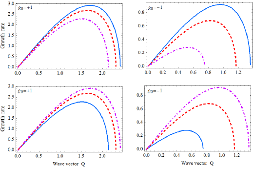
Figure 5: (Color online) The MI gain as produced by Eq. (35) for three values of the imprint parameter $\beta$, with $\phi_{0}=1$ and $q=2$. The top panel includes three values of $\beta>\beta_{c}=-0.5$: $\beta=-0.4$, $0.3$, and $0.2$ (the blue, red, and green lines, respectively). The bottom panel includes three values of $\beta<\beta_{c}=-0.5$: $\beta=-0.8$, $0.7$, and $0.6$ (the blue, red, and green lines, respectively). The left and right panels correspond to the focusing and defocusing nonlinearities, respectively. The figure reproduces known results for MI produced by the derivative NLS equation with constant coefficients Kamchatnov .

III.2.3 Modulational instability in the inhomogeneous cubic derivative NLS equation with the HO potential

To examine MI in the general case of Eq. (25), Ref. 3.33b made use of the modified lens transformation (LT),

$$\psi(x,t)=\frac{1}{\ell(t)}\phi(X,T)\exp[if(t)x^{2}+\eta(t)],$$ (36)

where $T=T(t)$, $\ell(t)$, $\eta(t)$, and $f(t)$ are real functions of time, and $X(x,t)=x\ell^{-1}(t)$. Originally, LT was introduced by Talanov Talanov as an invariant transformation for the 2D NLS equation, which changes the scale of the coordinates and adds the radial chirp (a phase term quadratic in the radial coordinate) to the wave function. The action of LT on the wave function is similar to the result of the ray propagation of the field governed by geometric optics. The significance of LT is stressed by its compatibility with adiabatic variation of the wave function governed by the cubic NLS equation, and with the dynamics driven by the critical collapse in 2D Gadi ; Fibich . Furthermore, LT applies as well to the 2D NLS equation including the isotropic HO potential Gadi .

To preserve the scaling of Eq. (25) we set

$$\frac{dT}{dt}=\frac{1}{\ell^{2}(t)}.$$ (37)

Demanding that

$$\frac{df}{dt}+4f^{2}+\alpha=0,$$ (38a)

$$4f(t)-\frac{1}{\ell}\frac{d\ell}{dt}=0,$$ (38b)

$$\frac{d\eta}{dt}+2f(t)-\frac{1}{\ell}\frac{d\ell}{dt}=0,$$ (38c)

$$\beta(t)=\widetilde{g}(t)f^{-1}(t)/8,$$ (38d)

and inserting ansatz (36) in Eq. (25) leads to

$$i\frac{\partial\phi}{\partial T}+\frac{\partial^{2}\phi}{\partial X^{2}}+\lambda_{0}(T)\left|\phi\right|^{2}\phi+i\lambda(T)\frac{\partial(|\phi|^{2}\phi)}{\partial X}=0,$$ (39)

where real functions of time are

$$\lambda_{0}(T)=\widetilde{g}_{0}(t)\exp[2\eta(t)],\quad\lambda(T)=4\,\frac{\beta(t)}{\ell(t)}\exp[2\eta(t)].$$ (40)

Thus, the invariance of the inhomogeneous cubic derivative NLS equation with respect to LT is maintained.

Solving Eqs. (38b), (38c) and (37) in terms of $f(t)$ yields

$$\ell(t) = \ell(0)\exp\biggl{(}4\int_{0}^{t}f(\upsilon)\,d\upsilon\biggr{)},$$ (41a)

$$\eta(t) = 2\int_{0}^{t}f(\upsilon)\,d\upsilon+\eta(0),$$ (41b)

$$T(t) = \ell^{-2}(0)\int_{0}^{t}\exp\biggl{(}-8\int_{0}^{s}f(\upsilon)\,d\upsilon\biggr{)}ds+T(0).$$ (41c)

Thus, the problem of finding time-dependent parameters $$\ell(t) \eta(t) T(t)$$, , and is reduced to solving the Riccati equation (38a).

According to ansatz (36) $\eta(t)$ affects the total number of atoms (the norm of the wave function), $N=\int_{\mathrm{R}}\left|\psi\right|^{2}dx=\ell^{-1}(t)\exp[\eta(t)]\int_{\mathrm{R}}\left|\phi\right|^{2}dX$, if $\ell^{-1}(t)\exp[\eta(t)]\neq\text{constant.}$ According to Eq. (41b), $\exp[\eta(t)]=\exp[2\int_{0}^{t}f(\upsilon)\,d\upsilon+\eta(0)]$, which means that $N$ exponentially grows if $f(t)$, the solution of the Riccati equation (38a), is positive, and exponentially decays if $f(t)$ is negative. In other words, positive $f(t)$ represents the feeding of atoms into the condensate, while negative $f(t)$ implies loss of atoms. While $f(t)$ depends on the strength of the HO trap, $\alpha(t)$, its sign is independent of the sign of $\alpha(t)$. For example, if $\alpha=-\alpha_{0}^{4}$ is a negative constant (which corresponds to the confining HO potential), then $f=\pm\alpha_{0}^{2}/2$ are two particular solutions of the Riccati equation (38a).

To investigate MI for the derivative NLS equation (39) with variable coefficients, Ref. 3.33b introduced perturbed solutions as

$$\phi=\left[\phi_{0}+\varepsilon(X,T)\right]\exp\biggl{[}-iQX-i\int_{0}^{T}\Omega(\upsilon)\,d\upsilon\biggr{]},$$ (42)

where $\Omega(T)$ is a real time-dependent function representing the nonlinear frequency shift, $\phi_{0}$ is a real constant, $Q$ is the wave number of the carrier, and $\varepsilon(X,T)$ is a small perturbation. Substituting ansatz (42) into Eq. (39), linearizing it with respect to the small perturbation, and substituting

$$\Omega(T)=Q^{2}-\lambda_{0}(t)\phi_{0}^{2}-Q\phi_{0}^{2}\lambda(t),$$ (43)

one obtains

$$i\,\frac{\partial\varepsilon}{\partial T}+\frac{\partial^{2}\varepsilon}{\partial X^{2}}+2i\left(\lambda\phi_{0}^{2}-Q\right)\,\frac{\partial\varepsilon}{\partial X}+i\lambda\phi_{0}^{2}\frac{\partial\varepsilon^{\ast}}{\partial X}+\phi_{0}^{2}\left(\lambda_{0}+\lambda Q\right)\left(\varepsilon+\varepsilon^{\ast}\right),$$ (44)

where $\ast$ stands for the complex conjugation. Solutions to Eq. (44) are sought for as

$$\varepsilon=U_{1}\exp\biggl{(}iKX-i\int_{0}^{T}\omega(\upsilon)\,d\upsilon\biggr{)}+U_{2}^{\ast}\exp\biggl{(}-iKX+i\int_{0}^{T}\omega^{\ast}(\upsilon)\,d\upsilon\biggr{)},$$ (45)

where $KX-\int_{0}^{T}\omega(\upsilon)\,d\upsilon$ is the modulation phase in which $K$ and $\omega$ are the wavenumber and the complex frequency of the perturbation, $U_{1,2}$ being complex amplitudes. MI sets in if frequency $\omega$ has a nonzero imaginary part. Inserting expression (45) into Eq. (44) yields the time-dependent dispersion relation,

$$\left[\omega-2K\left(\lambda\phi_{0}^{2}-Q\right)\right]^{2}-K^{2}\left[\allowbreak K^{2}+\phi_{0}^{2}\left(\lambda^{2}\phi_{0}^{2}-\allowbreak 2Q\lambda-2\lambda_{0}\right)\right]=0.$$ (46)

For $\omega$ to have a nonzero imaginary part, it is necessary and sufficient to have

$$\allowbreak K^{2}+\phi_{0}^{2}\left(\lambda^{2}\phi_{0}^{2}-\allowbreak 2Q\lambda-2\lambda_{0}\right)<0.$$ (47)

Inequality (47) is the MI criterion for the cubic derivative NLS equation (39). If the criterion holds, the local MI gain is given by

$$\left|\text{Im}\,\omega(t)\right|=\left|K\right|\sqrt{\phi_{0}^{2}\left[2Q\lambda(t)+2\lambda_{0}(t)-\lambda^{2}(t)\phi_{0}^{2}\right]-K^{2}}.$$ (48)

A particularly simple and interesting case is one with constant $\lambda_{0}$ and $\lambda$. Then it follows from Eqs. (37)-(38d) that $\beta\$is constant, while $\alpha(t)$ and $\widetilde{g}_{0}(t)$ satisfy the nonlinear second-order ODE,

$$\widetilde{g}_{0}\frac{d^{2}\widetilde{g}_{0}}{dt^{2}}-2\left(\frac{d\widetilde{g}_{0}}{dt}\right)^{2}-4\alpha\widetilde{g}_{0}^{2}=0.$$ (49)

Thus, in the special case of constant $\lambda_{0}$, $\lambda$ and $\beta$, the problem of finding $\ell(t)$, $\eta(t)$, and $T(t)$ amounts to solving Eq. (49). The simplest possibility is to solve it for $\alpha(t)$ if $\widetilde{g}_{0}(t)$ is known. For instance, $\widetilde{g}_{0}(t)=\widetilde{a}_{0}\exp\left(\widetilde{\lambda}t\right)$ produces constant $\alpha=-\widetilde{\lambda}^{2}/4.$

Following Ref. 2.3 , one of the most interesting cases in the setting with the HO potential is the one with

$$\alpha(t)=A(t+t^{\ast})^{-2},$$ (50)

for real constants $A$ and $t^{\ast}$ in Eq. (21), which determine, respectively, the strength of the potential and its width at $t=0$. Inserting expression (50) in Eq. (49) yields

$$\widetilde{g}_{0}(t)=\frac{4\lambda_{0}\beta}{\lambda\ell(0)}\left(\frac{t+t^{\ast}}{t^{\ast}}\right)^{m},\text{ \ }m=\frac{-1\pm\sqrt{1-16A}}{2}.$$ (51)

For $\widetilde{g}_{0}(t)$ to be a real function of time $t$, strength $A$ of the magnetic trap $\alpha(t)$, defined by Eq. (50), must satisfy condition $A<1/16$, which allows one to investigate MI for both the confining and expulsive potentials ($A<0$ and $A>0$, respectively). Note that $t^{\ast}<0$ describes BEC in a shrinking trap, while $t^{\ast}>$ $0$ corresponds to a broadening condensate. Inserting expressions (51) in the system of Eqs. (38a)-(38d) determines all time-dependent parameters; in particular, $T(t)=t^{\ast}\left(2m+1\right)^{-1}\ell^{-2}(0)\left[(t/t^{\ast}+1)^{2m+1}-1\right]$. To secure the variation of $T$ from zero to infinity, it is necessary to take $m=(-1+\sqrt{1-16A}\,)/2$ and $m=(-1-\sqrt{1-16A})/2$ in the cases of the broadening and shrinking trap, respectively. In the latter case, we focus on $t$ varying from $0$ to $-t^{\ast}$, to provide the variation of $T$ from $0$ to $+\infty$.

In the case of constant $\lambda_{0}$ and $\lambda$, the MI gain is time-independent, but it depends on the phase-imprint parameter $\beta$:

$$\left|\text{Im}\,\omega(\beta)\right|=\left|K\right|\sqrt{\phi_{0}^{2}\left[-\lambda^{2}(\beta)\phi_{0}^{2}+2Q\lambda(\beta)+2\lambda_{0}\right]-K^{2}}.$$ (52)

It is evident that the variation of the gain, controlled by $\beta$, may significantly modify the instability domain and bring new effects. In fact, to different values of $\beta$ there correspond different instability diagrams, depending on whether $\lambda(\beta)$ is positive or negative. Negative $\lambda(\beta)$ softens the instability, while $\lambda(\beta)>0$ enhances it. This behavior is shown in Fig. 6, which displays the MI gain provided by Eq. (52) as a function of perturbation wavenumber $K$, for three values of $\lambda(\beta)<0$ (plot (a)), and three values of $\lambda(\beta)>0$ (plot (b)). In Fig. 6(a) corresponding to $\lambda(\beta)<0$, it is easy to see that the gain decreases with the growth of parameter $\lambda$, while in Fig. 6(b), with $\lambda(\beta)>0$, the gain increases with the growth of $\lambda$.

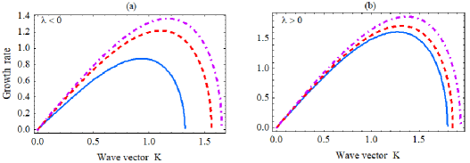
Figure 6: (Color online) The MI gain produced by Eq. (52) for three positive and three negative values of the imprint parameter $\lambda(\beta)$. (a): $\lambda(\beta)=-0.5$ (the solid line), $\lambda(\beta)=-0.25$ (the dashed line), and $\lambda(\beta)=-0.125$ (the dotted-dashed line); (b): $\lambda(\beta)=0.125$ (the solid line), $\lambda(\beta)=0.25$ (the dashed line), and $\lambda(\beta)=0.50$ (the dotted-dashed line). Other parameters are $Q=1$, $\phi_{0}=1$, and $\lambda_{0}=3/2$. The results are reproduced from Ref. 3.33b .

The results for constant $\lambda_{0}$ and $\lambda$ can be summarized as follows. For the occurrence of MI of CW solutions $\phi=\phi_{0}\exp\left(-iQX-i\left[Q^{2}-\lambda_{0}\phi_{0}^{2}-Q\phi_{0}^{2}\lambda\right]T\right)$, it is necessary and sufficient for wavenumber $K$ of the modulation perturbation to satisfy the MI criterion (47). Moreover, for given $\phi_{0}$, $Q$, and $\lambda_{0}$, the imprint parameter $\beta$ should be chosen such that $\lambda^{2}(\beta)\phi_{0}^{2}-2Q\lambda(\beta)-2\lambda_{0}<0.$

Next, it is relevant to look at the case when at least either $\lambda_{0}$ or $\lambda$ is not constant. As in the previous case, if the HO potential is considered with the same time dependence of the strength as in Eq. (50) with $A<1/16$, one can find a particular solution of Riccati equation (38a) in the form of

$$f(t)=B(t+t^{\ast})^{-1},\quad B=\frac{1\pm\sqrt{1-16A}}{8}.$$ (53)

With expression (53), the corresponding solution of Eq. (38a) reads

$$f(t)=\frac{1-4B+CB\left(1-8B\right)(t+t^{\ast})^{8B-1}}{C\left(1-8B\right)(t+t^{\ast})^{8B}+4(t+t^{\ast})},$$ (54)

where $C=\left[1-4B-4f(0)t^{\ast}\right]/\left[f(0)\left(1-8B\right)(t^{\ast})^{8B}-B\left(1-8B\right)(t^{\ast})^{8B-1}\right]$. Using Eqs. (50) and (53), one obtain the following time dependence of the parameters, cf. Eqs. (38a)-(38d):

$$\ell(t) = \ell(0)\left(\frac{t+t^{\ast}}{t^{\ast}}\right)^{4B},$$ (55a)

$$\eta(t) = 2B\ln\left|\frac{t+t^{\ast}}{t^{\ast}}\right|+\eta(0),$$ (55b)

$$\beta(t) = \frac{\widetilde{g}(t)(t+t^{\ast})}{8B},$$ (55c)

$$T(t) = \frac{1}{\ell(0)\left(1-4B\right)}\left[\left(t+t^{\ast}\right)\left(\frac{t^{\ast}}{t+t^{\ast}}\right)^{4B}-t^{\ast}\right].$$ (55d)

It follows from Eqs. (55a)-(55d) that $$\beta(t) \widetilde{g}(t) t^{\ast}>0 B<1/4 \ell(0) T(t) 0 +\infty t^{\ast}<0 \ell(0) B>1/4 t 0\leq t<t^{\ast} 0<T(t)<+\infty$$ is no longer a free parameter, as it depends of . In the case of (broadening condensate), it is reasonable to take ; a proper choice of then ensures the variation of from to . For BECs in the shrinking trap (), the appropriate choice of and demonstrates that the variation of in interval corresponds to .

In the case when, at least, either $\lambda_{0}$ or $\lambda$ is not constant, the MI gain given by Eq. (48) is time-dependent. In this situation, the variation of the gain, related to the sign of $t^{\ast}$ (recall that $t^{\ast}<0$ or $t^{\ast}>0$ determines, respectively, the shrinking or expanding trap), may significantly affect the MI domain and introduce new effects. The instability is enhanced or attenuated by $t^{\ast}<0$ or $t^{\ast}>0$, respectively, as shown in Fig. 7. The figure displays the MI gain produced by Eq. (48), as a function of perturbation wavenumber $K$, for three negative and three positive values of $t^{\ast}$, in plots 7(a) and (b), respectively. In Fig. 7(a), corresponding to the shrinking trap ($t^{\ast}<0$), one easily sees that the gain indeed increases with $t^{\ast}$, while in Fig. 7(b), obtained for the broadening trap ($t^{\ast}>0$), the gain decreases as $t^{\ast}$ increases. The plots in this figure are produced with $\widetilde{g}_{0}(t)=2\exp\left(0.5t\right)$ and $\widetilde{g}(t)=2\exp\left(-t\right)$.

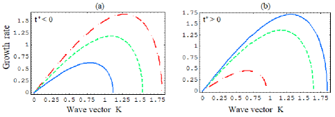
Figure 7: (Color online) The MI gain produced by Eq. ( 48) for three positive and three negative values of $t^{\ast}$ at time $t=0$. (a): The case of the shrinking trap with $t^{\ast}=-0.6$, $-0.4$, and $-0.2$ (the solid, dashed, and dotted-dashed lines, respectively). (b) The case of the broadening trap with $t^{\ast}=0.1$, $0.2$, $0.4$ (the solid, dashed, and dotted-dashed lines, respectively). Other parameters are $Q=1$, $\phi_{0}=1$, $A=-1$, $\ell(0)=1$, $\eta(0)=0$, $\widetilde{g}_{0}(t)=2\exp\left(0.5t\right)$, $\widetilde{g}(t)=2\exp\left(-t\right)$, $B=(1+\sqrt{17}\,)/8$ for plots (a), and $B=(1-\sqrt{17}\,)/8$ for (b). The results are reproduced from Ref. 3.33b .

The analysis makes it clear that the simplest and most interesting case in the setting with the time-dependent HO potential is the one with the inverse-square time dependence of the trap strength, as defined by Eq. (50) with $A<1/16$. In this case, the modified LT demonstrates the equivalence of the setting to the cubic derivative NLS equation. In this case, the coefficients of the cubic derivative NLS equation are either constant or time dependent, suggesting that frequencies of eigenmodes of the modulational perturbations are either constant or effectively time-dependent.

III.3 Matter-wave solitons of the cubic inhomogeneous NLS equation (20) with the spatiotemporal HO potential (21)

As said above, the condition of the transformability to the cubic derivative NLS with constant coefficients, where the MI analysis has been performed in the complete form, makes it most relevant to consider in Eq. (20) with the spatiotemporal potential (21), taken with $\alpha(t)=A(t+t^{\ast})^{-2}$ and $A<1/16$. The present subsection, following Ref. 3.33b , addresses this case in the analytical form under the assumption that $\lambda_{0}$ and $\lambda$ in Eq. (40) are constant.

The starting point is the CW solution of Eq. (39),

$$\phi(X,T)=\phi_{0}\exp\left[-ik_{0}X+i\left(\lambda_{0}\phi_{0}^{2}+k_{0}\lambda\phi_{0}^{2}-k_{0}^{2}\right)T\right].$$ (56)

Writing a solution of Eq. (39) in the Madelung form,

$$\phi(X,T)=R(X,T)\exp\left[i\Phi(X,T)\right],$$ (57)

one arrives at the following system of equations for the real amplitude and phase:

$$\left\{\begin{array}[]{r}-R\partial\Phi/\partial T+\partial^{2}R/\partial X^{2}-R\left(\partial\Phi/\partial X\right)^{2}-\lambda R^{3}\partial\Phi/\partial X+\lambda_{0}R^{3}=0,\\ \partial R/\partial T+2\left(\partial\Phi/\partial X\right)\left(\partial R/\partial X\right)+R\partial^{2}\Phi/\partial X^{2}+3\lambda R^{2}\partial R/\partial X=0.\end{array}\right.$$ (58)

Further, the CW solution (56) suggests to look for a solution to Eqs. (58) in the following traveling-wave form:

$$\left\{\begin{array}[]{l}R(X,T)=\phi_{0}+\rho(z=X-\upsilon T),\\ \Phi(X,T)=-k_{0}z+\varphi(z)+\left(\lambda_{0}\phi_{0}^{2}+\lambda k_{0}\phi_{0}^{2}-k_{0}^{2}-k_{0}\upsilon\right)T,\end{array}\right.$$ (59)

with arbitrary velocity $\upsilon$. Inserting ansatz (59) in the system of equations (58), and integrating the second equation yields

$$\frac{d\varphi}{dz}=\frac{C_{0}}{\left(\phi_{0}+\rho\right)^{2}}+\frac{\left(\upsilon+2k_{0}\right)}{2}-\frac{3\lambda}{4}\left(\phi_{0}+\rho\right)^{2},$$ (60)

where $C_{0}$ is a constant of integration. Inserting this expression for $d\varphi/dz$ into the first equation yields

$$\left(\frac{d\zeta}{dz}\right)^{2}=\widetilde{\alpha}\zeta^{4}+4\widetilde{\beta}\zeta^{3}+6\widetilde{\gamma}\zeta^{2}+4\widetilde{\delta}\zeta+\widetilde{\epsilon}\equiv f(\zeta),$$ (61)

where

$$\left.\begin{array}[]{l}\zeta(z)=\left(\phi_{0}+\rho(z)\right)^{2},\text{ }\widetilde{\alpha}=-\lambda^{2},\text{ }\widetilde{\beta}=\left(\lambda\upsilon-2\lambda_{0}\right)/4,\text{ }\widetilde{\epsilon}=-4C_{0}^{2},\\ \widetilde{\gamma}=\left[4\lambda_{0}\phi_{0}^{2}+2\lambda\left(2k_{0}\phi_{0}^{2}-C_{0}\right)-4\upsilon k_{0}-\upsilon^{2}-4k_{0}^{2}\right]/6,\end{array}\right.$$ (62)

$\widetilde{\delta}$ and $C_{0}$ being two arbitrary real constants of integration. The general solution of Eq. (61) with coefficients (62) can be obtained in terms of the Weierstrass’ elliptic function $\wp(z;g_{2},g_{3})$ 3.37 ; 3.38 :

$$\zeta(z)=\zeta_{0}+\frac{\sqrt{f(\zeta_{0})}\,\frac{d}{dz}\wp(z;g_{2},g_{3})+\frac{1}{2}f^{\prime}(\zeta_{0})\left[\wp(z;g_{2},g_{3})-\frac{1}{24}f^{\prime\prime}(\zeta_{0})\right]+\frac{1}{24}f(\zeta_{0})f^{\prime\prime\prime}(\zeta_{0})}{2\left[\wp(z;g_{2},g_{3})-\frac{1}{24}f^{\prime\prime}(\zeta_{0})\right]^{2}-\frac{1}{48}f(\zeta_{0})f^{(IV)}(\zeta_{0})},$$ (63)

where $\zeta_{0}$ is an arbitrary real constant, and the prime stands for $d/dz$ (recall $f(\zeta)$ is defined in Eq. (61)). Invariants $g_{2}$ and $g_{3}$ of function $\wp(z;g_{2},g_{3})$ are related to coefficients of $f(\zeta)$ as 3.37

$$g_{2}=\widetilde{\alpha}\widetilde{\epsilon}-4\widetilde{\beta}\widetilde{\delta}+3\widetilde{\gamma}^{2},\quad g_{3}=\widetilde{\alpha}\widetilde{\gamma}\widetilde{\epsilon}+2\widetilde{\beta}\widetilde{\gamma}\widetilde{\delta}-\widetilde{\alpha}\widetilde{\delta}^{2}-\widetilde{\gamma}^{3}-\widetilde{\epsilon}\widetilde{\beta}^{2}.$$ (64)

The discriminant $\Delta$ of the Weierstrass’ elliptic function $\wp(z;g_{2},g_{3})$,

$$\Delta=g_{2}^{3}-27g_{3}^{2},$$ (65)

is suitable to classify the behavior of the solution $\zeta(\xi)$ and to discriminate between periodic and solitary-wave solutions 3.38 . If $\Delta=0$, $g_{2}\geq 0$, and $g_{3}\leq 0$, $\zeta(\xi)$ is a solitary wave given by

$$\zeta(z)=\zeta_{0}+\frac{f^{\prime}(\zeta_{0})}{4\left[e_{1}-\frac{1}{24}f^{\prime\prime}(\zeta_{0})+3e_{1}\text{{cosech}}^{2}\left(\sqrt{3e_{1}}\,z\right)\right]},$$ (66)

where $e_{1}=\left(-g_{3}\right)^{1/3}$. Below, for simplicity, constants of integration are set as $\widetilde{\delta}=\widetilde{\epsilon}=0$. In this case, $g_{2}=3\widetilde{\gamma}^{2},\quad g_{3}=-\widetilde{\gamma}^{3}$, and $\Delta=0$. Then Eq. (66) defines solitary-wave solutions if and only if $\widetilde{\gamma}>0$ and $2\widetilde{\beta}^{2}-3\widetilde{\alpha}\widetilde{\gamma}\geq 0$. The physical solution (66) must be nonnegative and bounded. Considering properties of $f(\zeta)$ 3.39 , one obtains conditions, expressed in terms of coefficients of the basic equation, that determine the existence of the physical solutions, see Fig. 8 borrowed from Ref. 3.39 , which shows phase diagrams associated to the physical solutions for $\widetilde{\delta}=\widetilde{\epsilon}=0$.

According to Ref. 3.39 , solitary-wave solutions generated by Eq. (66) can be cast in the form of

$$\zeta_{\pm}(z)=\frac{\widetilde{\gamma}\left[2\widetilde{\beta}\pm\sqrt{4\widetilde{\beta}^{2}-6\widetilde{\alpha}\widetilde{\gamma}}\,\right]\biggl{[}3\widetilde{\gamma}^{2}+\left(\widetilde{\gamma}^{2}-1\right)\cosh^{2}\left(\sqrt{\frac{3}{2}\widetilde{\gamma}^{3}}\,z\right)\biggr{]}}{\left[-3\widetilde{\alpha}\widetilde{\gamma}^{3}+\left(4\widetilde{\beta}^{2}\pm 2\sqrt{4\widetilde{\beta}^{2}-6\widetilde{\alpha}\widetilde{\gamma}}-\widetilde{\alpha}\widetilde{\gamma}(5+\widetilde{\gamma})^{2}\right)\cosh^{2}\left(\sqrt{\frac{3}{2}\widetilde{\gamma}^{3}}\,z\right)\right]}.$$ (67)

These solutions correspond to two simple roots of the polynomial $f(\zeta)$ (provided that $4\widetilde{\beta}^{2}-6\widetilde{\alpha}\widetilde{\gamma}>0$), and are represented by phase diagrams (b), (c), (d), (f), (g), and (h) in Fig. 8 (see further details in Ref. 3.39 ).

It is necessary to address the condition of the non-negativeness of solutions (67). Here, two cases should be distinguished, namely, $\widetilde{\gamma}=1$, which corresponds to a bright solitary-wave solution, and $0<\widetilde{\gamma}\neq 1$, corresponding to both dark and bright solitary waves.

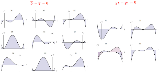
Figure 8: (Color online) Phase diagrams associated with real bounded solutions, given by Eqs. (63) and (61), with either $\widetilde{\delta}=\widetilde{\epsilon}=0$ (see also Eq. (67) for this case) or $\widetilde{\delta}\neq 0,$ $\widetilde{\epsilon}<0$, and $g_{2}=g_{3}=0$. Further details can be found in Refs. 3.40 and 3.39 for the right and left plots, respectively.

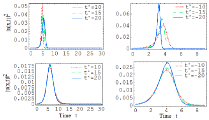
Figure 9: (Color online) Density plots $\left|u(x,t)\right|^{2}$ of solitary-wave solutions to Eq. (20) at $x=3$ for three values of parameter $t^{\ast}$ in potential (50), given by expression (67) for $\zeta_{+}$. The top and bottom panels correspond to the confining potential (with $A=-2$) and expulsive one (with $A=1/17$), respectively, while the left and right panels correspond to broadening shrinking traps, respectively. Values of other parameters are given in the text. The results are reproduced from Ref. 3.33b .

1. If $\widetilde{\gamma}=1$, solutions (67) is nonnegative if and only if

   $$\widetilde{\alpha}\left(2\widetilde{\beta}^{2}\pm\sqrt{4\widetilde{\beta}^{2}-6\widetilde{\alpha}}-18\widetilde{\alpha}\right)^{-1}<2/3$$ (68)

   and
   

   $$\left(2\widetilde{\beta}\pm\sqrt{4\widetilde{\beta}^{2}-6\widetilde{\alpha}}\,\right)\left(2\widetilde{\beta}^{2}\pm\sqrt{4\widetilde{\beta}^{2}-6\widetilde{\alpha}}-18\widetilde{\alpha}\right)>0.$$ (69)

   An example of the bright solitary-wave solution is obtained with parameters $\lambda_{0}=1$, $\phi_{0}=1$, $\upsilon=0.5$, $k_{0}=1$, and $\lambda=\allowbreak 2.0625$. With this set of parameters, $\zeta_{+}(z)$ satisfies all the needed conditions (reality, boundedness and non-negativeness). Figures 9, 10, and 11, respectively, show effects of  $t^{\ast}$, $A$ and $\beta$ on the density profile of the solitary-wave solution, $\left|u(x,t)\right|^{2}$, at $x=3$; here, $\ell(0)=1$ is set. In these three figures, left and right panels correspond, respectively, to the broadening and shrinking traps ($t^{\ast}>0$ and $t^{\ast}<0$, respectively), while top and bottom panels correspond to the confining and expulsive potentials $(A<0\$and $A>0$, respectively). At $x=3$, Fig. 9 shows the time evolution of density $\left|u(x,t)\right|^{2}$ for three different values of $t^{\ast}.$ As seen in the figure, in the case of the confining potential, the amplitude of the density profile decreases as $t^{\ast}$ increases for the broadening trap, and increases with the growth of $t^{\ast}$ for the shrinking trap. In the case of the expulsive potential, the profile’s amplitude increases with $t^{\ast}$ for both broadening and shrinking traps. Figure 10 depicts density $\left|u(x,t)\right|^{2}$ at $x=3$ for three different values of $A$. This figure shows that, for both the confining and expulsive potentials (the top and bottom plots, respectively), the profile’s amplitude decreases as $A$ increases, which happens for both the broadening and shrinking BEC traps (left and right plots, respectively). It is seen from Fig. 11, where density $\left|u(x,t)\right|^{2}$ at $x=3$ is depicted for different values of $\beta$, that, irrespective of the sign of $A$ (the confining or expulsive potential) and the sign of $t^{\ast}$ (the broadening or shrinking trap), the density-profile’s amplitude decreases with the increase of the imprint parameter $\beta$.

   

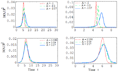
   Figure 10: (Color online) The same as in Fig. 9, but for three different values of parameter $A$ in potential (50). The top and bottom panels correspond to the confining and expulsive potential, respectively, while the left and right panels are associated, severally, with the broadening trap (for $t^{\ast}=10$) and the shrinking one (for $t^{\ast}=-10$). Typical values of other parameters are given in the text. The results are reproduced from Ref. 3.33b .

   

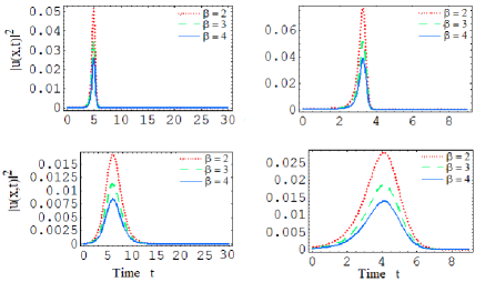
   Figure 11: (Color online) The same as in Figs. 9 and 10, but for three different values of the imprint parameter $\beta$ in Eq. (24b). The top and bottom panels correspond to the confining potential (with $A=-2$) and expulsive one (with $A=1/17$), respectively, while the left and right panels are associated, severally, with the broadening trap (for $t^{\ast}=10$) and the shrinking one (for $t^{\ast}=-10$). Typical values of other parameters are given in the text. The results are reproduced from Ref. 3.33b .

   

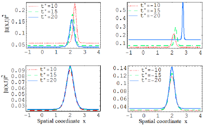
   Figure 12: (Color online) Density $\left|u(x,t)\right|^{2}$ at $t=4$, as given by solution (67), for three different values of parameter $t^{\ast}$ appearing in potential (50). The top and bottom panels correspond, severally, to the confining potential (with $A=-2$) and the expulsive one (with $A=1/17$), while the left and right panels are associated with the broadening and shrinking trap, respectively. Typical values of other parameters are given in the text. The results are reproduced from Ref. 3.33b .

2. If $0<\widetilde{\gamma}\neq 1$, solutions (67) are nonnegative if and only if the following three conditions are simultaneously satisfied: (i) $3\widetilde{\gamma}^{2}\left(1-\widetilde{\gamma}^{2}\right)^{-1}\leq 1$, (ii) $3\widetilde{\alpha}\widetilde{\gamma}^{3}\left(4\widetilde{\beta}^{2}\pm 2\sqrt{4\widetilde{\beta}^{2}-6\widetilde{\alpha}\widetilde{\gamma}}-\widetilde{\alpha}\widetilde{\gamma}(5+\widetilde{\gamma})^{2}\right)^{-1}<1$, and (iii)

   $$\widetilde{\gamma}\left(\widetilde{\gamma}^{2}-1\right)\left(2\widetilde{\beta}\pm\sqrt{4\widetilde{\beta}^{2}-6\widetilde{\alpha}\widetilde{\gamma}}\,\right)\left(4\widetilde{\beta}^{2}-\widetilde{\alpha}\widetilde{\gamma}(5+\widetilde{\gamma})^{2}\pm 2\sqrt{4\widetilde{\beta}^{2}-6\widetilde{\alpha}\widetilde{\gamma}}\,\right)>0.$$ (70)

   
   

   With parameters $\lambda_{0}=1$, $\phi_{0}=1$, $\upsilon=0.5$, $\lambda=\allowbreak 3.5625$, and $k_{0}=1$, conditions (i)–(iii) are simultaneously satisfied for $\zeta_{+}(z)$, providing an example of a dark solitary-wave solution to Eq. (61). For this set of parameters, density $\left|u\left(x,t\right)\right|^{2}$, associated with the solitary-wave solution (67), is depicted at $x=3$ in Figs. 9, 10, and 11, and at $t=4$ in Figs. 12, 13, and 14, to show the effect of  $t^{\ast}$, $A$, and $\beta$ on the solitary-wave shape. Here, $\ell(0)=1$ is used. In these figures, left and right panels correspond to the broadening and shrinking traps ($t^{\ast}>0$ and $t^{\ast}<0$, respectively), while top and bottom panels correspond to the confining and expulsive potential $(A<0\$and $A>0$, respectively). In particular, Fig. 12 shows, at time $t=4$, the spatial evolution of density $\left|u(x,t)\right|^{2}$ for three different values of $t^{\ast}$. As seen in the figure, the peak density in the case of confining potential decreases as $t^{\ast}$ increases for the broadening trap (the top panels), and increases with $t^{\ast}$ for the shrinking trap. In the case of the expulsive potential (the bottom panels), the peak density increases with $t^{\ast}$ for both the broadening and shrinking traps. Figure 13 depicts density $\left|u(x,t)\right|^{2}$ at $t=4$ for three different values of $A$. The figure demonstrates that, for both the confining and expulsive potentials, the peak density decreases as $A$ increases, which happens for both the broadening and shrinking traps. Figure 14, where density $\left|u(x,t)\right|^{2}$ is displayed at $t=4$ for different values of $\beta$, shows that, irrespective of the sign of $A$ (the confining or expulsive potential) and the sign of $t^{\ast}$ (the broadening or shrinking trap), the peak density decreases with the increase of imprint parameter $\beta$.

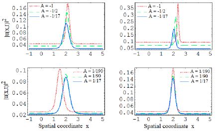
Figure 13: (Color online) The same as in Fig. 12, but for three different values of parameter $A$ in potential (50). The top and bottom panels correspond to the confining and expulsive potentials, respectively, while the left and right panels are associated, severally, with the broadening trap (for $t^{\ast}=10$) and the shrinking one (for $t^{\ast}=-10$), respectively. Values of other parameters are given in the text. The results are reproduced from Ref. 3.33b .

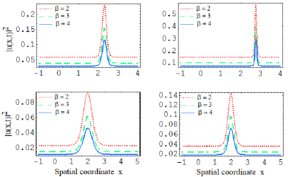
Figure 14: (Color online) The same as in Figs. 12 and 13, but for three different values of the imprint parameter $\beta$ in transformation (24b). The upper and lower panels correspond to the confining potential (with $A=-2$) and the expulsive one (with $A=1/17$), respectively, while the left and right panels are associated, severally, with yjr broadening trap (for $t^{\ast}=10$) and the shrinking one (for $t^{\ast}=-10$),. Typical values of other parameters are given in the text.

III.4 Conclusion of the section

In this section, MI of CW states is surveyed in the context of the inhomogeneous cubic NLS equations with the external potential. The motivation for this study was its link to BEC with the spatially modulated local nonlinearity. To make the investigation of MI possible for both attractive and repulsive nonlinearities, the inhomogeneous cubic NLS equation is first transformed into the inhomogeneous cubic derivative NLS equation, by means of the suitably designed PIT, applied to the wave function of the original cubic NLS equation. A modified LT is then used to cast the problem in the form in which the cubic derivative NLS equation has constant coefficients. For the strength of the magnetic trap modulated in time $\sim$ $(t+t^{\ast})^{-2}$ and the local time-dependent nonlinearity coefficient being a linear function of $x$, the resulting MI gain is either constant or time varying. The impact of both the PIT imprint parameter and trap parameter $t^{\ast}$ on the MI gain is considered. In the case of the constant MI gain, analytical matter-wave solitons of the inhomogeneous NLS equation under the consideration are presented, and the effect of the above-mentioned parameters on their shape is considered.

IV Collapse management for BEC with time-modulated nonlinearity

In this section we address the dynamics of 2D and 3D condensates with the nonlinearity coefficient, i.e., the scattering length of inter-atomic collision, subject to the time modulation imposed by the FR, which makes the coefficient a sum of constant and periodically oscillating terms. The respective results were obtained by means of VA and systematic direct simulations of the GP equation 3.1 -Itin . An averaging method can be used too, in the case of the rapid time modulation Baizakov . In the 2D case, all these methods reveal the existence of stable self-confined states in the free space (without an external trap), in agreement with similar results originally reported for (2+1)D spatial solitons in nonlinear optics 4.7 . In the 3D free space, the VA also predicts the existence of self-confined state without a trap Adhikari . In this case, direct simulations demonstrate that the stability is limited in time, eventually switching into collapse. Thus, a spatially uniform ac magnetic field, resonantly tuned to drive the periodic temporal modulation of the scattering length by means of FR, may play the role of an effective trap confining the condensate, and sometimes causing its collapse.

Results collected in this section are chiefly based on original works 4.7 , 3.1 , and Baizakov . Although these works were published quite some time ago, the findings reported in them are highly relevant to the topic of the present review article.

IV.1 The model and VA (variational approximation)

The starting point is the mean-field GP equation for the single-particle wave function in its usual form, cf. Eq. (1):

$$i\hbar\frac{\partial\psi(\mathbf{r,}t\mathbf{)}}{\partial t}=\left[-\frac{\hbar^{2}}{2m}\nabla^{2}+g\left|\psi(\mathbf{r,}t\mathbf{)}\right|^{2}\right]\psi(\mathbf{r,}t\mathbf{)}$$ (71)

with $g=4\pi\hbar^{2}a_{s}/m$, where $a_{s}$ and $m$ are the atomic scattering length and mass. Throughout this section, its is assumed the scattering length to be modulated in time, so that the nonlinearity coefficient in Eq. (71) takes the form of $g=g_{0}+g_{1}\sin\left(\chi t\right)$, where $g_{0}$ and $g_{1}$ are the amplitudes of the dc and ac parts, and $\chi$ is the ac-modulation frequency.

To stabilize the condensate, an external trapping potential is usually included. Nevertheless, it is omitted in Eq. (71) because it does not play an essential role in the present context. This is also the case in many other situations – for example, the formation of stable Skyrmions in two-component condensates is possible in the free space 4.1 . Indeed, it is demonstrated in some detail below that the temporal modulation of the nonlinearity coefficient, combining the dc and ac parts as in Eq. (72), may, in a certain sense, replace the trapping potential.

Equation (71) is cast in a normalized form by introducing a typical frequency, $\Omega=2gn_{0}/\hbar$, where $n_{0}$ is the largest value of the condensate density, and rescaling the time and space variables as $t^{\prime}=\Omega t$, $\mathbf{r}^{\prime}=\mathbf{r}\sqrt{2m\Omega/\hbar}$. This leads to the scaled equation for isotropic states (in which only the radial coordinate is kept, and the primes are omitted):

$$i\frac{\partial\psi(\mathbf{r,}t\mathbf{)}}{\partial t}=-\left(\frac{\partial^{2}}{\partial r^{2}}+\frac{D-1}{r}\frac{\partial}{\partial r}\right)\psi(r,t\mathbf{)}-\left[\lambda_{0}+\lambda_{1}\sin\left(\omega t\right)\right]\left|\psi(r,t\mathbf{)}\right|^{2}\psi(r,t\mathbf{)}.$$ (72)

Here $D=2$ or $3$ is the spatial dimension, and $\lambda_{0,1}\equiv-g_{0,1}/\left(\Omega\hbar\right)$, $\omega\equiv\chi/\Omega$. Note that $\lambda_{0}>0$ and $\lambda_{0}<0$ in Eq. (72) correspond to the self-focusing and self-defocusing nonlinearity, respectively. Additionally rescaling field $\psi$, $\left|\lambda_{0}\right|=1$ is set, so that $\lambda_{0}$ remains a sign-defining parameter.

As the next step, one applies VA to Eq. (72). This approximation was originally proposed by Anderson et al. 4.2 ; Anderson ; 4.4 for 1D temporal solitons, then for matter-wave solitons in BEC 4.3 , and later developed for multidimensional models Desaix ; 4.7 ; 3.1 . To apply the VA in the present case, one should use the Lagrangian density generating Eq. (72),

$$\mathcal{L}\left(\psi\right)=\frac{i}{2}\left(\frac{\partial\psi}{\partial t}\psi^{\ast}-\frac{\partial\psi^{\ast}}{\partial t}\psi\right)-\left|\frac{\partial\psi}{\partial r}\right|^{2}+\frac{1}{2}\lambda(t)\left|\psi\right|^{4},$$ (73)

where $\lambda(t)=\lambda_{0}+\lambda_{1}\sin\left(\omega t\right)$, and the asterisk stands for the complex conjugation. The variational ansatz for the wave function is chosen as the Gaussian 4.2 :

$$\psi_{G}(r,t)=A(t)\exp\left[-\frac{r^{2}}{2a^{2}(t)}+\frac{1}{2}ib(t)r^{2}+i\delta(t),\right]$$ (74)

where $A$, $a$, $b$, and $\delta$ are, respectively, the amplitude, width, chirp, and overall phase, which are assumed to be real functions of $t$. In fact, the Gaussian is the single type of the trial wave function which makes it possible to develop VA in the fully analytical form. A caveat is that, if the frequency of the ac drive resonates with a transition between the ground state of the condensate and a possible excited one (it definitely exists if the model includes a trapping potential), the single GP equation should be replaced by a system of coupled ones for the resonantly interacting states.

Following Ref. 4.4 , one inserts the ansatz in the Lagrangian density (73) and calculates the respective effective Lagrangian,

$$L_{\text{eff}}=C_{D}\int_{0}^{\infty}\mathcal{L}\left(\psi_{g}\right)r^{D-1}dr,$$ (75)

where $C_{D}=2\pi$ or $4\pi$ in the 2D or 3D cases, respectively. Finally, the evolution equations for the time-dependent parameters of ansatz (74) are derived from $L_{\text{eff}}$ using the corresponding Euler-Lagrange equations. Subsequent analysis, as well as the results of direct numerical simulations, is presented separately for the 2D and 3D cases.

IV.2 The two-dimensional case

We start the consideration with the 2D case, presenting, consecutively, results produced by VA, application of the averaging method to the GP equation, and results produced by numerical simulations. In particular, in the case of the high-frequency modulation, it is possible to apply the averaging method to the 2D equation (72), without using VA 3.1 ; Baizakov ; Abdullaev . The averaging method may also be applied to the 2D NLS equation with a potential rapidly varying in space, rather than in time, the main result being renormalization of parameters of the equation and a shift of the collapse threshold 4.5 . As shown below, rapid temporal modulation of the nonlinearity coefficient in the GP equation leads to nontrivial effects, such as generation of additional nonlinear-dispersive and higher-order nonlinear terms in the corresponding effective NLS equation, see, Eq. (92) below. These terms may essentially affect the dynamics of the collapsing condensate.

IV.2.1 The variational approximation

The calculation of the effective Lagrangian (75) for the 2D GP equation yields

$$L_{\text{eff}}^{(2D)}=\pi\left(-\frac{1}{2}a^{4}A^{2}\frac{db}{dt}-a^{2}A^{2}\frac{d\delta}{dt}-A^{2}-a^{4}A^{2}b^{2}+\frac{1}{4}\lambda(t)a^{2}A^{4}\right).$$ (76)

The Euler-Lagrange equations following from this Lagrangian yield the conservation of the total number of atoms $N$ in the condensate (represented by norm $N$ of the mean-field wave function),

$$\pi a^{2}A^{2}\equiv N=\text{ const},$$ (77)

expressions for the chirp and width,

$$\frac{da}{dt}=2ab\text{, }\frac{db}{dt}=\frac{2}{a^{4}}-2b^{2}-\frac{\lambda(t)N}{2\pi a^{4}},$$ (78)

and a closed-form evolution equation for the width:

$$\frac{d^{2}a}{dt^{2}}=\frac{2\left(2-\lambda(t)N/2\pi\right)}{a^{3}},$$ (79)

which may be rewritten as

$$\frac{d^{2}a}{dt^{2}}=\frac{-\Lambda+\epsilon\sin\left(\omega t\right)}{a^{3}},$$ (80)

where

$$\Lambda\equiv 2\left[\lambda_{0}N/(2\pi)-2\right],\text{ \ }\epsilon=-\lambda_{1}N/\pi.$$ (81)

In the absence of the ac component, i.e., $\epsilon=0$, Eq. (80) conserves the energy, $E_{\mathrm{2D}}=(1/2)\left[\left(da/dt\right)^{2}-\Lambda a^{-2}\right]$. Obviously, $E_{\mathrm{2D}}\rightarrow-\infty$ as $a\rightarrow 0$, if $\Lambda>0$, and $E_{\mathrm{2D}}\rightarrow+\infty$ as $a\rightarrow 0$, if $\Lambda<0$. This means that, in the absence of the ac component, the 2D pulse is expected to collapse at $\Lambda>0$, and spread out at $\Lambda<0$. The case of $\Lambda=0$ corresponds to the critical norm, realized by the above-mentioned TS Townes . Note that a numerically exact value of the critical norm is (in the present notation) $N=1.862$ Fibich , while the variational equation (81) yields $N=2$ (if $\lambda_{0}=+1$) Anderson .

If the ac component of the nonlinearity coefficient oscillates at a high frequency, one can set $a(t)=\overline{a}+\delta a$, with $\left|\delta a\right|<<\left|\overline{a}\right|$, where, $\overline{a}$ varies on a slow time scale and $\delta a$ is a rapidly varying function with zero mean value. Then, Eq. (80) can be treated analytically by means of the Kapitsa averaging method 3.1 ; Baizakov ; Abdullaev . After straightforward manipulations, an ODE system is derived for the slow and rapid variables:

$$\frac{d^{2}\overline{a}}{dt^{2}} = -\Lambda\left(\overline{a}^{-3}+6\overline{a}^{-5}\langle\delta a^{2}\rangle\right)-3\epsilon\langle\delta a\sin\left(\omega t\right)\rangle\overline{a}^{-4},$$ (82a)

$$\frac{d^{2}}{dt^{2}}\delta a = 3\delta a\Lambda\overline{a}^{-4}+\epsilon\sin\left(\omega t\right)\overline{a}^{-3},$$ (82b)

where $$\langle\cdots\rangle 2\pi/\omega$$ stands for averaging over period . Equation (82b) admits an obvious solution,

$$\delta a(t)=-\frac{\epsilon\sin\left(\omega t\right)}{\overline{a}^{3}\left(\omega^{2}+3\overline{a}^{-4}\Lambda\right)}.$$ (83)

Substituting Eq. (83) into Eq. (82a) yields the following final evolution equation for the slow variable:

$$\frac{d^{2}\overline{a}}{dt^{2}}=\overline{a}^{-3}\left[-\Lambda-\frac{3\Lambda\epsilon^{2}}{\left(\omega^{2}\overline{a}^{4}+3\Lambda\right)^{2}}+\frac{3}{2}\frac{\epsilon^{2}}{\omega^{2}\overline{a}^{4}+3\Lambda}\right].$$ (84)

To examine whether the collapse is enforced or inhibited by the ac component of the nonlinearity, one may look at Eq. (84) in the limit of $\overline{a}\rightarrow 0$, reducing the equation to

$$\frac{d^{2}\overline{a}}{dt^{2}}=\left(-\Lambda+\frac{\epsilon^{2}}{6\Lambda}\right)\overline{a}^{-3}.$$ (85)

It follows from Eq. (85) that, if the amplitude of the high-frequency ac component is large enough, viz., $\epsilon>6\Lambda^{2}$, the behavior of the condensate (in the limit of small $\overline{a}$) is exactly opposite to that which would be expected in the presence of the dc component only: in the case $\Lambda>0$, rebound occurs rather than the collapse, and vice versa in the case $\Lambda<0$.

On the other hand, in the limit of large $\overline{a}$ , Eq. (84) takes the asymptotic form of $d^{2}\overline{a}/dt^{2}=-\Lambda\overline{a}^{-3}$, which shows that the condensate remains self-confined in the case of $\Lambda>0$, i.e., if the norm exceeds the critical value. This consideration is relevant if $\overline{a}$, although being large, remains smaller than the limit imposed by an external trapping potential, should it be added to the model. Thus, these asymptotic results guarantee that Eq. (84) give rise to a stable behavior of the condensate, the collapse and decay (spreading out) being ruled out if

$$\epsilon>\sqrt{6}\Lambda>0.$$ (86)

To illustrate the above results in terms of the experimentally relevant setting – for example, for the condensate of ⁷Li with the critical number $\sim 1500$ atoms – one concludes that, for $1800$ atoms (i.e., $N/2\pi=2.2$) the stabilization requires to add the periodic modulation with amplitude $\epsilon=0.98$ (see Eq. (81) to the constant coefficient $\lambda_{0}=1$. In fact, conditions (86) ensure that the right-hand side of Eq. (84) is positive for small $\overline{a}$ and negative for large $\overline{a}$, hence Eq. (84) must give rise to a stable fixed point. Indeed, when conditions (86) hold, the right-hand side of Eq. (84) vanishes at exactly one fixed point,

$$\omega^{2}\overline{a}^{4}=\frac{3\epsilon^{2}}{4\Lambda}+\sqrt{3\left(\frac{3\epsilon^{4}}{16\Lambda^{2}}-1\right)}-3\Lambda,$$ (87)

which can be easily checked to be stable through the calculation of an eigenfrequency of small oscillations around it.

Direct numerical simulations of Eq. (80) produce results that are in exact agreement with those provided by the averaging method, i.e., a stable state with $\alpha(t)$ performing small oscillations around point (87) 3.1 ; Abdullaev . However, the 3D situation shows a drastic difference, see below.

For the sake of comparison with the results obtained in the 3D case, one also needs an approximate form of Eq. (84) valid in the limit of small $\Lambda$ (i.e., when norm is close to the critical value) and very large $\omega$:

$$\frac{d^{2}\overline{a}}{dt^{2}}=-\frac{\Lambda}{\overline{a}^{3}}+\frac{3}{2}\frac{\epsilon^{2}}{\omega^{2}\overline{a}^{7}}.$$ (88)

To estimate the value of the amplitude of the high-frequency ac component necessary to stop the collapse, note that a characteristic trap frequency is $\Omega\sim 100$ Hz, in physical units. Then, for a typical high modulation frequency $\sim 3$ kHz, the scaled one is $\omega\simeq 30$. If the norm is, for instance, $N/2\pi=2.2$, so that, according to Eq. (81), $\Lambda=0.4$ (this corresponds to the condensate of ⁷Li with $\simeq 1800$ atoms, the critical number being $\simeq 1500$), and the modulation parameters are $\lambda_{0}=1$, $\lambda_{1}=2.3$, $\epsilon=10$, then the stationary value of the condensate’s width, as obtained from Eq. (87), is $a_{\mathrm{st}}=0.8l$, where $l=\sqrt{m\Omega/\hbar}$ is the healing length.

Thus the analytical approach, based on VA and the assumption that the norm slightly exceeds the critical value, leads to an important prediction: in the case of the 2D GP equation, the ac component of the nonlinearity, acting jointly with the dc one corresponding to the attraction, may replace the collapse by a stable soliton-like oscillatory state that confines itself without the trapping potential. It is relevant to mention, once again, that a qualitatively similar result, viz., the existence of stable periodically oscillating spatial cylindrical solitons in a bulk nonlinear-optical medium consisting of alternating layers with opposite signs of the Kerr coefficient, was reported in Ref. 4.7 , where this result was obtained in a completely analytical form on the basis of the variational approximation, and was confirmed by direct simulations.

IV.2.2 Averaging of the 2D GP (Gross-Pitaevskii) equation and Hamiltonian

Here, it is assumed that the ac frequency $\omega$ is large, and the 2D GP equation (72) is rewritten in the following form,

$$i\frac{\partial\psi}{\partial t}+\nabla^{2}\psi+\lambda(\omega t)\left|\psi\right|^{2}\psi=0.$$ (89)

To derive an equation governing the slow variations of the field, one can use the multiscale approach, writing the solution as an expansion in powers of $1/\omega$ and introducing slow temporal variables, $T_{k}\equiv\omega^{-k}t$, $k=0,$ $1,$ $2,$ $...$, while the fast time is $\zeta=\omega t$. Thus, the solution is sought for as

$$\psi(r,t)=A(r,T_{k})+\omega^{-1}u_{1}(\zeta,A)+\omega^{-2}u_{2}(\zeta,A)+\cdots,$$ (90)

with $\langle u_{k}\rangle=0$, where $\langle\cdots\rangle$ stands for the average over the period of the rapid modulation, and $\lambda_{0}=1$ is assumes (i.e., the dc part of the nonlinearity coefficient corresponds to attraction between the atoms).

Following the procedure developed in Ref. 4.8 , one first finds the first and second corrections,

$$u_{1}=-i\left(\mu_{1}-\langle\mu_{1}\rangle\right)\left|A\right|^{2}A,\text{ \ }\mu_{1}\equiv\int_{0}^{\zeta}\left[\lambda(\tau)-\langle\lambda_{1}\rangle\right]d\tau,$$

$$u_{2}=\left(\mu_{2}-\langle\mu_{2}\rangle\right)\left[2i\left|A\right|^{2}A_{t}+iA^{2}A_{t}^{\ast}+\nabla^{2}(\left|A\right|^{2}A)\right]$$ (91)

$$-\left|A\right|^{4}A\left\{\frac{1}{2}\left[\left(\mu_{1}-\langle\mu_{1}\rangle\right)^{2}-2M\right]+\langle\lambda\rangle\left(\mu_{2}-\langle\mu_{2}\rangle\right)\right\}.$$

In Eq. (91), $\mu_{2}\equiv\int_{0}^{\zeta}\left(\mu_{1}-\langle\mu_{1}\rangle\right)ds$, and $M=\left(1/2\right)\left(\langle\mu_{1}^{2}\rangle-\langle\mu_{1}\rangle^{2}\right)=\left(1/2\right)\left(\langle\lambda^{2}\rangle-1\right)$ (recall $\lambda_{0}=1$ was set). Using these results, one obtains the following evolution equation for the slowly varying field $A(x,T_{0})$, derived at order $\omega^{-2}:$

$$i\frac{\partial A}{\partial t}+\nabla^{2}A+\left|A\right|^{2}A+2M\left(\frac{\epsilon}{\omega}\right)^{2}\left(\left|A\right|^{6}A-3\left|A\right|^{4}\nabla^{2}A\right)+2\left|A\right|^{2}\nabla^{2}\left(\left|A\right|^{2}A\right)+A^{2}\nabla^{2}\left(\left|A\right|^{2}A^{\ast}\right)=0,$$ (92)

where $\epsilon$ is the same amplitude of the ac component as in Eq. (81). Note that Eq. (92) is valid in both 2D and 3D cases. In either case, it can be represented in the quasi-Hamiltonian form

$$\left[1+6M\left(\frac{\epsilon}{\omega}\right)^{2}\left|A\right|^{4}\right]\frac{\partial A}{\partial t}=-i\frac{\delta H_{q}}{\delta A^{\ast}},$$ (93)

$$H_{q}=\int dV\left[\left|\nabla A\right|^{2}-2M\left(\frac{\epsilon}{\omega}\right)^{2}\left|A\right|^{8}-\frac{1}{2}\left|A\right|^{4}+4M\left(\frac{\epsilon}{\omega}\right)^{2}\left|\nabla\left(\left|A\right|^{2}A\right)\right|\right],$$ (94)

where $dV$ is the infinitesimal volume in the 2D or 3D space. It immediately follows from Eq. (93) and the reality of the (quasi-)Hamiltonian (94) that it is a dynamical invariant, i.e., $dH_{q}/dt=0$.

For further analysis of the 2D case, it is relevant apply the modulation theory developed in Ref. 4.9 , according to which the solution is searched for in the form of a modulated TS. The above-mentioned TS is a solution of the 2D NLS equation in the form of $\psi(r,t)=\exp\left(it\right)R_{T}(r)$, where function $R_{T}(r)$ is the solution of the boundary-value problem,

$$\frac{d^{2}R_{T}}{dr^{2}}+\frac{1}{r}\frac{dR_{T}}{dr}-R_{T}+R_{T}^{3}=0,\text{ }\left.\frac{dR_{T}}{dr}\right|_{r=0}=0,\text{ }\left.R_{T}(r)\right|_{r=\infty}=0.$$ (95)

For this solution, norm $N$ and the Hamiltonian $H$ take the well-known values,

$$N_{T} \equiv \int_{0}^{\infty}R_{T}^{2}(r|)rdr=N_{c}\approx 1.862,$$

$$H_{T} = \int_{0}^{\infty}\left[\left(\frac{dR_{T}}{dr}\right)^{2}-\frac{1}{2}R_{T}^{4}(r)\right]rdr=0.$$ (96)

The averaged variational equation (92) indicates an increase of the critical norm for the collapse, as opposed to the classical value in Eq. (96). Using relation (90), we find

$$N_{\text{crit}}=\int_{0}^{\infty}\left|\psi\right|^{2}rdr=N_{T}+2\mathrm{I}M\left(\frac{\epsilon}{\omega}\right)^{2},$$ (97)

where $\mathrm{I}=11.178$. This increase of the critical norm is similar to the well-known energy enhancement of dispersion-managed solitons in optical fibers with periodically modulated dispersion 4.6 .

Another nontrivial perturbative effect is the appearance of a nonzero value of the phase chirp in the soliton. The mean value of the chirp is defined as

$$b=\frac{\int_{0}^{\infty}\text{{Im}}\left[\left(\partial\psi/\partial r\right)\psi^{\ast}\right]rdr}{\int_{0}^{\infty}r^{2}dr\left|\psi\right|^{2}}.$$ (98)

Making use of expression (91) for the first correction leads to

$$b = -\left(\epsilon/\omega\right)BM\left(\mu_{1}-\langle\mu_{1}\rangle\right),$$ (99)

$$B \equiv 3\frac{\int_{0}^{\infty}rdrR^{2}(R^{\prime})^{2}-(1/4)\int_{0}^{\infty}drR^{4}}{\int_{0}^{\infty}r^{2}drR^{2}}\approx 0.596.$$ (100)

To develop a general analysis, it is assumed that the solution with the norm close to the critical value may be approximated as a modulated TS, i.e.,

$$A(r,t)\approx\left[a(t)\right]^{-1}R_{T}\left[r/a(t)\right]\exp\left(iS\right),\text{ \ }S=\sigma(t)+\frac{r^{2}}{4a}\frac{da}{dt},\text{ \ }\frac{d\sigma}{dt}=a^{-2}$$ (101)

with some function $a(t)$. If the initial norm is close to the critical value, i.e., when $\left|N-N_{c}\right|<<N_{c}$, the method worked out in Ref. 4.9 makes it possible to derive an evolution equation for $a(t)$, starting from approximation (101). The evolution equation for the width is

$$a^{3}a_{tt}=-\beta_{0}+\frac{\epsilon^{2}}{4M_{0}\omega^{2}}f_{1}(t),$$ (102)

where

$$\beta_{0}=\beta(0)-\frac{\epsilon^{2}}{4M_{0}\omega^{2}}f_{1}(0),\text{ \ }\beta(0)=\frac{N-N_{c}}{M_{0}},\text{ \ }M_{0}\equiv\frac{1}{4}\int_{0}^{\infty}r^{3}drR_{T}^{2}\approx 0.55,$$ (103)

with an auxiliary function

$$f_{1}(t)=2a(t)\text{{Re}}\left[\frac{1}{2\pi}\int\int dxdyF(A_{T})\exp\left[-iS\right]\left\{R_{T}+\rho\nabla R_{R}(\rho)\right\}\right].$$ (104)

For the harmonic modulation, the equation in the lowest-order approximation takes the form of

$$\frac{d^{2}a}{dt^{2}}=-\frac{\Lambda_{1}}{a^{3}}+\frac{C\epsilon^{2}}{\omega^{2}a^{7}},$$ (105)

where $\Lambda_{1}=\left(N-N_{c}\right)/M_{0}-C\epsilon^{2}/(\omega^{2}a_{0}^{4})$ and $C$ is defined as 3.1

$$C\equiv\frac{3}{M_{0}}\int_{0}^{\infty}d\rho\left[2\rho R_{T}^{4}\left(R_{T}^{\prime}\right)^{2}-\rho^{2}R_{T}^{3}\left(R_{T}^{\prime}\right)^{3}-\frac{1}{8}\rho R_{T}^{8}\right]\approx 39.$$ (106)

Thus the averaged equation predicts the arrest of the collapse by the rapid modulations of the nonlinear term in the 2D GP equation. The comparison of Eq. (105) with its counterpart (88), which was derived by means of averaging the VA-generated equation (80), shows that both approaches lead to the same behavior near the collapse threshold, numerical coefficients in the second terms being different due to the different profiles of the Gaussian and TS.

It is relevant to estimate the fixed point as per numerical simulations performed in Ref. 4.10 . In that work, the stable propagation of solitons has been observed for two-step modulation of the nonlinearity coefficient in the 2D NLS equation: $\lambda=1+\epsilon$ at $0<t<T$, and $\lambda=1-\epsilon$ at $T<t<2T$. The parameters in the numerical simulations were taken as $T=\epsilon=0.1,$ $N/(2\pi)=11.726/(2\pi)$, with the critical number $N_{c}=11.68/(2\pi)$. For these values, one has $a_{c}=0.49$, which agrees with the value $a_{c}\approx 0.56$ produced by numerical simulations.

Instead of averaging Eq. (72), one can apply the averaging procedure, also based on representation (90) for the wave function, directly to the Hamiltonian of Eq. (72). As a result, the averaged Hamiltonian is found in the form of

$$\overline{H}=\int\int dxdy\left[\left|\nabla A\right|^{2}+2M\left(\frac{\epsilon}{\omega}\right)^{2}\left|\nabla\left(\left|A\right|^{2}A\right)\right|^{2}-\frac{1}{2}\left|A\right|^{4}-6M\left(\frac{\epsilon}{\omega}\right)^{2}\left|A\right|^{8}\right].$$ (107)

A possibility to arrest the collapse, in the presence of the rapid periodic modulation of the nonlinearity strength, can be explained with the help of this Hamiltonian. To this end, following the pattern of the virial estimates 4.11 , one notes that, if a given field configuration has compressed itself to a spot with size $\rho$, where the amplitude of the $A$ field is $\sim\aleph$, the conservation of norm $N$ (which may be applied to field $A$ through relation (90)) yields relation

$$\aleph^{2}\rho^{D}\sim N,$$ (108)

$D$ being the space dimension. On the other hand, the same estimate for the strongest collapse-driving and collapse-arresting terms (the fourth and second terms, respectively, in expression (107)), $H_{-}$ and $H_{+}$, in the Hamiltonian yields

$$H_{-}\sim-\left(\frac{\epsilon}{\omega}\right)^{2}\aleph^{8}\rho^{D},\text{ \ \ }H_{+}\sim\left(\frac{\epsilon}{\omega}\right)^{2}\aleph^{6}\rho^{D-2}.$$ (109)

Eliminating the amplitude from Eqs. (109) by means of relation (108), one concludes that, in the case of the catastrophic self-compression of the field in the 2D space, $\rho\rightarrow 0$, both terms $H_{\pm}$ asymptotically scale as $\rho^{-5}$, hence the collapse may be arrested, depending on details of the configuration. However, in the 3D case the collapse-driving term diverges as $\rho^{-9}$, while the collapse-arresting one scales $\sim\rho^{-8}$ at $\rho\rightarrow 0$, hence in this case the collapse cannot be prevented.

Lastly, it is relevant to mention that, although the quasi-Hamiltonian (94) is not identical to the averaged Hamiltonian (107), the virial estimate applied to $H_{q}$ yields exactly the same result: the collapse can be arrested in the 2D case, but not in the 3D one.

IV.2.3 Numerical simulations

The existence of stable self-confined soliton-like oscillating states, predicted by means of the analytical approximations in region (86), when the dc part of the nonlinearity corresponds to self-attraction, and the amplitude of the ac component is not too small, was checked by simulations of the 2D equation (72). It was quite easy to confirm this prediction (in the case $\lambda_{0}=-1$, i.e., when the dc component of the nonlinearity corresponds to repulsion, the direct simulations always show a decay (spreading out) of the condensate, which also agrees with the above predictions). A typical example of the formation of a self-confined state, supported by the combination of the self-focusing dc and sufficiently strong ac components of the nonlinearity in the absence of an external trap, is displayed in Fig. 15. The left panel shows the radial profile of a collapsing state at $t\approx 0.3$ in the absence of the ac term. In the presence of this term, the right panel shows that the pulse is stabilized for about $40$ ac-modulation periods, after which it decays (possible eventual decay on a very long time scale was numerically investigated, in a detailed form, in Ref. Itin ). Note the generation of radiation, attached to the main body as a tail, which is a result of self-adjustment of the input to the modulation.

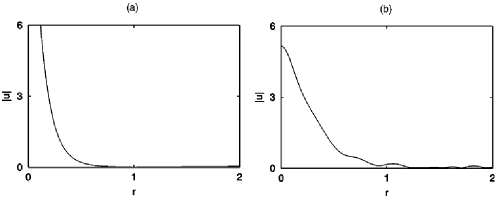
Figure 15: A typical example of the formation of a self-confined condensate in simulations of the 2D equation (72). Panel (a) shows the collapsing state in the absence of the ac modulation at $t\approx 0.3$. Panel (b) shows the radial profile of the stable state formed by the same input at $t\approx 0.6$, in the presence of the ac term in the nonlinearity coefficient. The parameters are $\lambda_{0}=2.4$, $\lambda_{1}=0.85$, $\omega=100\pi$, and $N=5$. The results are reproduced from Ref. 3.1 .

IV.3 The 3D GP model

To address the situation in the case of the 3D equation (72), it is relevant, similar to the 2D case, to separately consider results produced by the analytical approximations, i.e., VA and averaging, and by direct simulations.

IV.3.1 VA and averaging

Calculating effective Lagrangian (75) in the case of the 3D GP equation yields

$$L_{\text{eff}}^{(3D)}=\frac{1}{2}\pi^{\frac{3}{2}}A^{2}a^{3}\left[-\frac{3}{2}a^{2}\frac{db}{dt}-2\frac{d\delta}{dt}+\frac{1}{2\sqrt{2}}\lambda(t)A^{2}-\frac{3}{a^{2}}-3b^{2}a^{2}\right].$$ (110)

The Euler-Lagrange equations produced by this Lagrangian yield the norm conservation,

$$\pi^{\frac{3}{2}}A^{2}a^{3}\equiv N=\text{ const,}$$ (111)

relations including the chirp,

$$\frac{da}{dt}=2ab\text{, }\frac{db}{dt}=\frac{2}{a^{4}}-2b^{2}-\frac{\lambda(t)N}{2\sqrt{2}\pi^{\frac{3}{2}}a^{5}},$$ (112)

and the evolution equation for the width of the condensate,

$$\frac{d^{2}a}{dt^{2}}=\frac{4}{a^{3}}-\frac{\lambda(t)}{2\sqrt{2}\pi^{\frac{3}{2}}}\frac{N}{a^{4}},$$ (113)

which is different from its counterpart (79) corresponding to the 2D case.

Proceeding as in the 2D case, one renormalizes the amplitudes of the dc and ac components of the nonlinearity as $\Lambda\equiv\lambda_{0}N/\sqrt{2\pi^{3}}$ and $\epsilon\equiv-\lambda_{1}N/\sqrt{2\pi^{3}}$, and cast Eq. (113) in the scaled form

$$\frac{d^{2}a}{dt^{2}}=\frac{4}{a^{3}}+\frac{-\Lambda+\epsilon\sin\left(\omega t\right)}{a^{4}}.$$ (114)

In the absence of the ac term, i.e., $\epsilon=0$, Eq. (114) conserves the energy

$$E_{\text{{3D}}}=\frac{1}{2}\left(\frac{da}{dt}\right)^{2}+2a^{-2}-\frac{1}{3}\Lambda a^{-3}.$$ (115)

This expression shows that $E_{\text{{3D}}}\rightarrow-\infty$ as $a\rightarrow 0$, if $\Lambda>0$, and $E_{\text{{3D}}}\rightarrow+\infty$ as $a\rightarrow 0$ if $\Lambda<0$, which corresponds to the collapse or decay of the pulse, respectively.

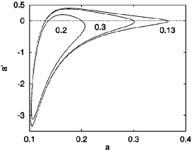
Figure 16: The Poincaré section in the plane of ($a,da/dt$ ) for $\Lambda=-1$, $\epsilon=100$, $\omega=10^{4}\pi$, generated by the numerical solution of the variational equation (114) with different initial conditions (see the text). The results are reproduced from Ref. 3.1 .

Prior to applying the averaging procedure, Eq. (114) can be solved numerically, without averaging, to show that there is a region in the parameter space where the condensate, which would decay under the action of the repulsive dc nonlinearity ($\Lambda<0$), may be stabilized by the ac component, provided that its amplitude is sufficiently large. The behavior of the solutions is displayed in Fig. 16, by means of the Poincaré section in the phase plane of ($a,da/dt$), for $\Lambda=-1$, $\epsilon=100$, $\omega=10^{4}\pi$, and initial conditions $a(t=0)=0.3$, $0.2$, or $0.13$ and $da/dt(t=0)=0$. As seen in Fig. 16, in all the cases the solution remains bounded with quasiperiodic oscillations, avoiding the collapse or decay.

In fact, the corresponding stability region in the parameter plane ($\omega/\pi,\epsilon$) is small, see Fig. 17. It is also seen that the frequency and amplitude of the ac component need to be large enough to maintain the stability. Note that, for frequencies larger than $10^{6}\pi$, the width of the condensate $a(t)$ assumes very small values in the course of the evolution (as predicted by VA), suggesting that the collapse may occur in the solution of the full 3D equation (72). The stability is predicted by VA only for $\Lambda<9$, i.e., for the repulsive dc component of the nonlinearity coefficient. In the opposite case, VA predicts solely the collapse.

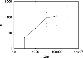
Figure 17: The region in the ($\epsilon,\omega/\pi$) parameter plane where the numerical solution of Eq. (114) with $\Lambda=-1$ predicts stable quasiperiodic solutions in the 3D case. Crosses mark points where stable solutions were actually obtained. Stars correspond to minimum values of the ac-component’s amplitude $\epsilon$ eventually leading to the collapse of the solution of the full partial differential equation (72) with $\Lambda=-1$. The results are reproduced from Ref. 3.1 .

As $\omega$ is large enough in the stability region shown in Fig. 17, it seems natural to apply the averaging method to this case too. Similar to how it is outlined above in the 2D case, the rapidly oscillating correction $\delta a(t)$ to the solution can be found, cf. Eq. (83):

$$\delta a=-\frac{\epsilon\sin\left[\omega t\right]\overline{a}}{\omega^{2}\overline{a}^{5}-12\overline{a}+4\Lambda},$$ (116)

and the resulting evolution equation for the slow variable $\overline{a}(t)$ is

$$\frac{d^{2}\overline{a}}{dt^{2}}=\overline{a}^{-4}\left[4\overline{a}^{4}-\Lambda+\frac{2\epsilon^{2}}{\omega^{2}\overline{a}^{5}-12\overline{a}+4\Lambda}+\epsilon^{2}\frac{6\overline{a}-5\Lambda}{\left(\omega^{2}\overline{a}^{5}-12\overline{a}+4\Lambda\right)^{2}}\right].$$ (117)

In the limit $\overline{a}\rightarrow 0$, Eq. (117) takes the form of

$$\frac{d^{2}\overline{a}}{dt^{2}}=\left[-\Lambda+\frac{3\epsilon^{2}}{16\Lambda}\right]\overline{a}^{-4}.$$ (118)

Equation (118) predicts one property of the 3D model correctly, viz., in the case $\Lambda<0$ and with a sufficiently large amplitude of the ac component ($\epsilon>(4/\sqrt{3})\left|\Lambda\right|$), it follows from Eq. (118) that collapse takes place instead of spreading out. However, other results following from the averaged equation (117) are wrong, as compared to those produced by simulations of the full variational equation (114), which are displayed above (see Figs. 16 and 17). In particular, detailed analysis of the right-hand side of Eq. (117) shows that it does not predict a stable fixed point for $\Lambda<0$, and does predict it for $\Lambda>0$, exactly opposite to what is revealed by the simulations of Eq. (114). The failure of the averaging approach in this case may be explained by the existence of singular points in Eqs. (116) and (117) (for both $\Lambda>0$ and $\Lambda<0$), at which the denominator $\omega^{2}\overline{a}^{5}-12\overline{a}+4\Lambda$ vanishes. Note that, in the 2D case with $\Lambda>0$, for which the stable state was found (see Eq. (86)), the corresponding Eq. (84) did not have singularities.

IV.3.2 Direct simulations of the GP equation in the 3D case

Comparison of the results produced by VA with direct simulations of the 3D version of the radial equation (72) is necessary.

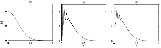
Figure 18: The evolution of the density radial profile, $\left|u(r)\right|^{2}$, in the presence of the strong and fast ac modulation ($\omega=10^{4}\pi$, $\epsilon=90$). The profiles of $\left|u(r)\right|^{2}$ are shown at different times: $t=0.007$ (a), $0.01$ (b), and $0.015$ (c). The results are reproduced from Ref. 3.1 .

In the absence of the ac component, i.e., $\epsilon=0$ and under the condition $\Lambda<0$, the simulations show straightforward decay. If an ac component with a sufficiently large amplitude is added, transient stabilization of the condensate takes place, roughly similar to how it is predicted by the solution of the variational equation (114). However, the stabilization is not permanent: the wave function begins to develop small-amplitude short-scale variations around the center, and after about $50$ periods of the ac modulation, the collapse takes place.

An example of this behavior is displayed in Fig. 18, for $N=1$, $\Lambda=-1$, and $\omega=10^{4}\pi$. Figure 18 shows radial density profiles $\left|u(r)\right|^{2}$ at different instants of time. Results presented in Fig. 18 is typical for the 3D case with $\Lambda<0$. The eventual collapse that takes place in this case is a nontrivial finding, as it occurs despite the fact that the dc part of the nonlinearity drives the condensate towards spreading out. Therefore, a basic characteristic of the system is a dependence of the minimum ac amplitude $\epsilon$, which gives rise to the collapse at fixed $\Lambda=-1$, versus ac frequency $\omega$. Several points marked by stars show this dependence in Fig. 17. It is natural that the minimum value of $\epsilon$ necessary for the collapse grows with $\omega$. On the other hand, for $\omega$ not too large, this minimum value is small, as even small $\epsilon$ is sufficient to push the state into the collapse during the relatively long half-period when the sign of the net nonlinearity coefficient $\lambda(t)$ is positive, see Eq. (89).

In the case of $\Lambda>0$ the collapse cannot be predicted, in agreement with the analysis developed above on the basis of the Hamiltonian of the averaged version of the GP equation, which showed that the collapse could not be arrested in the 3D case, provided that the amplitude of the ac component was large enough. This result also accords with the findings of direct simulations of the propagation of localized 3D spatiotemporal pulses in the above-mentioned model of the nonlinear-optical medium consisting of alternating layers with opposite signs of the Kerr coefficient: on the contrary to the stable 2D spatial solitons, the 3D “light bullets” can never be stable in that model.

IV.4 Conclusion of the section

The dynamics of both 2D and 3D BEC is considered in the case when the nonlinearity coefficient in the GP equation contains constant (dc) and time-variable (ac) parts. This may be achieved in the experiment by means of a resonantly tuned ac magnetic field, through FR. Using VA, directly simulating the GP equation, and applying the averaging procedure to it without the use of VA, one concludes that, in the 2D case, the ac component of the nonlinearity makes it possible to maintain the condensate in a stable self-confined state without an external trap, which agrees with known results reported for spatial solitons in nonlinear optics. In the 3D case, VA also predicts a stable self-confined state of the condensate without a trap, provided that the constant part of the nonlinearity corresponds to repulsion between atoms. However, in this case direct simulations reveal that the stability of the self-confined condensate is limited in time. Eventually, collapse takes place, despite the fact that the dc component of the nonlinearity is repulsive. Thus, the conclusion is that the spatially uniform ac magnetic field, resonantly tuned to affect the scattering length via FR, may readily play the role of an effective trap that confines the condensate, and sometimes enforces its collapse.

V Soliton stability in two-component BEC under temporal modulation

In the present section, we address the dynamics of a binary condensate in an expulsive time-varying HO potential with time-varying intrinsic attractive interactions, governed by an integrable system of two 1D GP equations. In this model, the strength of the attractive nonlinearity exponentially decays with time, hence solitons are also subject to decay. Nevertheless, it is shown that the robustness of bright solitons can be enhanced, making their lifetime longer, by matching the time dependence of the interaction strength to the time modulation of the strength of the HO potential. The nonlinearity coefficient can be made time-dependent through FR, which helps to choose the time-modulation pattern corresponding to the integrable system. A conclusion is that the expulsive time-modulated HO potential, combined with the modulated nonlinearity, may sustain stable BEC, while it quickly decays in the time-independent potential. The analytical results predicting this behavior are confirmed by numerical simulations. Furthermore, it is demonstrated that the addition of noise does not impact the BEC stability in the expulsive time-dependent potential.

Results presented in this section are based on Ref. add8 .

V.1 The physical model and the Lax pair

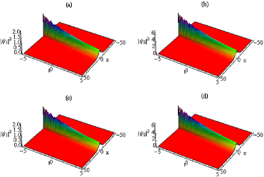
Figure 19: (Color online) (a,b): The analytical soliton solution of Eqs. (120) under the integrability condition (136), with $g(t)$ taken as per Eq. (141) (and $\lambda^{2}=1/16$). (c,d): The numerically generated counterpart of the same solution. The results are reproduced from Ref. add8 .

The model to be studied in this section pertains to two-component BEC, with equal atomic masses and attractive interactions in both components (such as the condensate composed of two hyperfine states of ⁷Li 4.12 or ⁸⁵Rb 4.13 atoms), trapped in the HO potential. The mean-field evolution of the setting is governed by coupled 1D GP equations, written in the scaled form as

$$i\frac{\partial\psi_{j}}{\partial t}=\left(-\frac{1}{2}\frac{\partial^{2}}{\partial x^{2}}+b_{jj}\left|\psi_{j}\right|^{2}+b_{j3-j}\left|\psi_{3-j}\right|^{2}+\frac{1}{2}\Omega_{j}^{2}(t)x^{2}\right)\psi_{j}=0,\text{\ }j=1,2,$$ (119)

where $\psi_{j}$ is the mean-field wave function of the $j$-th component subject to the normalization condition $\int_{-\infty}^{+\infty}\left|\psi_{1}\right|^{2}dx=1$ and $\int_{-\infty}^{+\infty}\left|\psi_{2}\right|^{2}dx=N_{2}/N_{1}$. The intrinsic interactions in Eq. (119) are controlled by the SPM and XPM coefficients, $b_{jj}=4a_{jj}N_{i}/r_{\perp}$ and $b_{jk}=4a_{jk}N_{i}/r_{\perp}$, where $a_{jj}$ and $a_{jk}$ are the respective scattering lengths, and $r_{\perp}$ is the transverse-component radius. In the section, the symmetric system is considered, with $b_{11}=b_{22}=b_{21}=b_{12}\equiv-g$, and $\Omega_{j}^{2}(t)=\omega_{j}^{2}(t)/\omega_{\perp}^{2}$, where $\omega_{j}$ and $\omega_{\perp}$ represent, respectively, frequencies of the trapping potential in the longitudinal and transverse directions. Time $t$ and coordinate $x$ are measured in units of $2/\omega_{\perp}$ and $r_{\perp}$ $=\sqrt{\hbar/\left(m\omega_{\perp}\right)}$, respectively.

Further, assuming $\Omega_{1}^{2}(t)=\Omega_{2}^{2}(t)\equiv-\lambda^{2}(t)$ (i.e., the confining and expulsive signs of the potential correspond to $\lambda^{2}<0$ and $\lambda^{2}>0$, respectively), and allowing the interaction coefficient $g(t)$ and potential strength $\lambda^{2}(t)$ to vary in time, Eq. (119) takes the following form (with additional rescaling $t\rightarrow 2t$):

$$i\frac{\partial\psi_{j}}{\partial t}+\frac{\partial^{2}\psi_{j}}{\partial x^{2}}+2g(t)\left(\left|\psi_{j}\right|^{2}+\left|\psi_{3-j}\right|^{2}\right)\psi_{j}+\lambda^{2}(t)x^{2}\psi_{j}=0,\text{ }j=1,2.$$ (120)

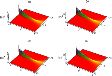
Figure 20: (Color online) The same as in Fig. 19, but $g(t)$ given by Eq. (142), with $\lambda^{2}=1/4$. The results are reproduced from Ref. add8 .

In this system the nonlinearity takes the Manakov’s form 4.14 , which is a well-known necessary condition for the integrability of the system. In what follows, we consider the case of $g(t)>0$, which corresponds to the attractive sign of the SPM and XPM interactions. Under the special integrability condition imposed on $g(t)$ and $\lambda(t)$, system (120) admit a representation in the form of the Lax pair,

$$\left.\begin{array}[]{c}\Phi_{x}+U\Phi=0,\\ \Phi_{t}+V\Phi=0,\end{array}\right.$$ (121)

where $\Phi=(\phi_{1},\phi_{2},\phi_{3})^{T}$ is the three-component Jost function, and the operators are

$$U = \left(\begin{array}[]{ccc}i\zeta(t)&Q_{1}&Q_{2}\\ -Q_{1}^{\ast}&-i\zeta(t)&0\\ -Q_{2}^{\ast}&0&-i\zeta(t)\end{array}\right),$$ (122d)

$$V = \left(\begin{array}[]{ccc}v_{11}&v_{12}&v_{13}\\ v_{21}&v_{22}&v_{23}\\ v_{31}&v_{32}&v_{33})\end{array}\right),$$ (122h)

with

$$v_{11} = -i\zeta^{2}(t)+i\Gamma(t)x\zeta(t)+\frac{i}{2}Q_{1}Q_{1}^{\ast}+\frac{i}{2}Q_{2}Q_{2}^{\ast},$$ (123)

$$v_{12} = \Gamma(t)xQ_{1}-\zeta(t)Q_{1}+\frac{i}{2}\frac{\partial Q_{1}}{\partial x},$$ (124)

$$v_{13} = \Gamma(t)xQ_{2}-\zeta(t)Q_{2}+\frac{i}{2}\frac{\partial Q_{2}}{\partial x},$$ (125)

$$v_{21} = \Gamma(t)xQ_{1}^{\ast}+\zeta(t)Q_{1}^{\ast}+\frac{i}{2}\frac{\partial Q_{1}^{\ast}}{\partial x},$$ (126)

$$v_{22} = i\zeta^{2}(t)-i\Gamma(t)x\zeta(t)-\frac{i}{2}Q_{1}Q_{1}^{\ast},$$ (127)

$$v_{23} = -\frac{i}{2}Q_{2}Q_{1}^{\ast},$$ (128)

$$v_{31} = -\Gamma(t)xQ_{2}^{\ast}+\zeta(t)Q_{2}^{\ast}+\frac{i}{2}\frac{\partial Q_{2}^{\ast}}{\partial x},$$ (129)

$$v_{32} = -\frac{i}{2}Q_{1}Q_{2}^{\ast},$$ (130)

$$v_{33} = i\zeta^{2}(t)-i\Gamma(t)x\zeta(t)-\frac{i}{2}Q_{2}Q_{2}^{\ast},$$ (131)

$$Q_{1} = \frac{1}{\sqrt{g(t)}}\psi_{1}(x,t)\exp\left(\frac{i}{2}\Gamma(t)x^{2}\right),$$ (132)

$$Q_{2} = \frac{1}{\sqrt{g(t)}}\psi_{2}(x,t)\exp\left(\frac{i}{2}\Gamma(t)x^{2}\right).$$ (133)

The compatibility condition, $(\Phi_{x})_{t}=(\Phi_{t})_{x}$, leads to the zero-curvature equation, $U_{t}-V_{x}+[U,V]$ $=0$, which is tantamount to the integrable system (120), provided that the spectral parameter $\zeta(t)$ obeys the following nonisospectral condition:

$$\zeta(t)=\mu\exp\left(-\int\Gamma(t)dt\right),$$ (134)

where $\mu$ is a hidden complex constant and $\Gamma(t)$ is an arbitrary function of time, which is related to the trap’s strength:

$$\lambda^{2}(t)=\Gamma^{2}(t)-\frac{d\Gamma}{dt},$$ (135)

and $\lambda(t)$ is related to the variable interaction strength $g(t)$ by the integrability condition:

$$\lambda^{2}(t)g^{2}(t)=2\left(\frac{dg}{dt}\right)^{2}-g(t)\frac{d^{2}g}{dt^{2}}.$$ (136)

Thus, the system of GP equations (120) is integrable if $\lambda(t)$ and $g(t)$ satisfy the integrability condition (136). For the time-independent trap, $\lambda(t)=$const $\equiv$ $c_{1}$, Eq. (136) yields $g(t)=\exp\left(c_{1}t\right)$. In what follows, we focus on the consideration of the integrable system satisfying this condition. If the rigorous integrability condition is slightly broken, the result depends on the accumulation of the deviation from the integrability over a characteristic time scale, $T$, of the dynamical regime. Namely, if the deviation from the integrability is characterized by difference $\Delta\lambda(t)$ from the value imposed by Eq. (136), the condition for the system to remain close to the integrability is

$$\left|\int_{0}^{T}\Delta\lambda(t)dt\right|\ll 1.$$ (137)

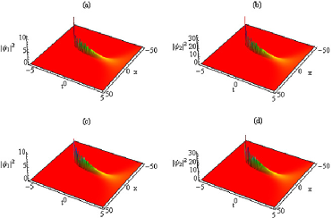
Figure 21: (Color online) The same as in Fig. 19, but for $g(t)$ given by Eq. (143), with $\lambda^{2}=0.81$. The figure is borrowed from Ref. add8 .

It is important to mention that one can convert the integrable system of the coupled GP equations, defined by Eqs. (120) and (136), into the usual Manakov’s model with constant coefficients (120) by a suitable transformation. Nevertheless, the direct formulation of the integrability formalism in the form of Eqs. (122d), (122h), and (136) is quite useful, as it makes it possible to apply the gauge-transformation method for generating multisoliton solutions, and it may also be used for the search of more general integrable systems.

V.2 Analytical and numerical results for two-component bright solitons in the integrable system

With the help of the gauge-transformation approach, bright solitons of the system of GP equations (120), subject to the integrability condition (136), can be looked for as

$$\psi_{1}^{(1)} = \frac{2}{\sqrt{g(t)}}\varepsilon_{1}^{(1)}\frac{\beta_{1}(t)}{\cosh\theta_{1}}\exp\left[i\left(-\xi_{1}+\Gamma(t)x^{2}/2\right)\right],$$ (138a)

$$\psi_{2}^{(1)} = \frac{2}{\sqrt{g(t)}}\varepsilon_{2}^{(1)}\frac{\beta_{2}(t)}{\cosh\theta_{1}}\exp\left[i\left(-\xi_{1}+\Gamma(t)x^{2}/2\right)\right],$$ (138b)

where

$$\theta_{1} = 2\beta_{1}x+4\int\alpha_{1}\beta_{1}dt-2\delta_{1},$$ (139)

$$\xi_{1} = 2\alpha_{1}x+2\int(\alpha_{1}^{2}-\beta_{1}^{2})dt-2\chi_{1},$$ (140)

with $\alpha_{1}=\alpha_{10}\exp\left[\int\Gamma(t)dt\right]$, $\beta_{1}=\beta_{10}\exp\left[\int\Gamma(t)dt\right]$, while $\delta_{1}$ and $\chi_{1}$ are arbitrary parameters, and $\varepsilon_{1,2}^{(1)}$ are coupling coefficients, which are subject to constraint $\left|\varepsilon_{1}^{(1)}\right|^{2}+\left|\varepsilon_{2}^{(1)}\right|^{2}=1$.

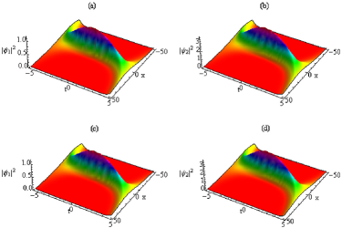
Figure 22: (Color online) (a,b): The analytical soliton solution of Eqs. (120), given by Eqs. (138a) and (138b), with $g(t)$ and $\lambda^{2}(t)$ taken as per Eqs. (144) and (145). (c,d): The numerically generated counterpart of the same solution. The results are reproduced from Ref. add8 .

To start the analysis of particular solutions relevant for the physical realization of the system, one can switch off the time dependence of the HO trap and adopt the dependence of the nonlinearity coefficient in the form of

$$g(t)=0.5\exp\left(-0.25t\right),$$ (141)

for which Eq. (136) renders the HO potential time-independent and expulsive, with $\lambda^{2}=1/16>0$. The corresponding density profile of the analytical solution, given by Eqs. (135) and (138a), (138b), is displayed in Figs. 19(a,b). Its counterpart produced by numerical simulations of Eq. (120) is shown in Figs. 19(c,d). In these figures one observes perfect agreement between the analytical and numerical solutions, which also implies stability of the analytical solution. If the time-modulated interaction strength (141) is replaced by

$$g(t)=0.5\exp\left(-0.5t\right),$$ (142)

for which Eq. (136) yields a stronger expulsive potential, with $\lambda^{2}=1/4$, the condensate quickly spreads out, as shown by the analytical solution in Figs. 20(a,b), and its numerical counterpart in Figs. 20(c,d). As seen in Fig. 21, this trend (including the stability of the analytical solution) continues if the time dependence (142 is replaced by

$$g(t)=0.5\exp\left(-0.9t\right),$$ (143)

for which Eq. (136) yields $\lambda^{2}=0.81$.

Figure 23: The same as in Fig. 22, but for $g(t)$ and $\lambda^{2}(t)$ taken as per Eqs. (146) and (LABEL:lambdar). Note the essential difference of the spatiotemporal shape of the solution in comparison with that displayed in Fig. 22. The results are reproduced from Ref. add8 .

To enhance the stability of the condensates, one can switch on the time dependence of the HO strength, taking

$$g(t)=0.5\exp\left(-0.125t^{2}\right),$$ (144)

for which Eq. (136) yields the expulsive potential with strength

$$\lambda^{2}=1/4+t^{2}/16.$$ (145)

The corresponding analytical solution, generated by Eqs. (138a) and (138b) is displayed in Figs. 22(a,b). The correctness and stability of the analytical solution is corroborated by its numerical counterpart, as shown in Figs. 22(c,d). Further, for the much steeper modulation of the interaction coefficient, with

$$g(t)=0.5\exp\left(-2.5t^{2}\right),$$ (146)

the integrability condition (136) yields

$$\lambda^{2}=5+25t^{2}.$$ (147)

The corresponding analytical solution, given by Eqs. (138a) and (138b), and its numerical counterpart are displayed in Fig. 23. Note that this solution demonstrates non-monotonous evolution in time: the soliton’s wave fields shrink and then expand.

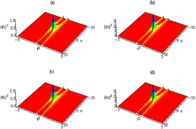
Figure 24: The same as in Fig. 23, but for $g(t)$ and $\lambda^{2}(t)$ given by Eqs. (148) and (149). The results are reproduced from Ref. add8 .

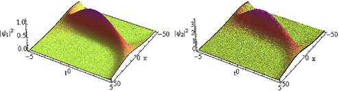
Figure 25: (Color online) The same as in Fig. 22(c,d), but in the case when strong white random noise, with a standard spectral width, is added to the simulations. The results are reproduced from Ref. add8 .

A still steeper modulation of the interaction coefficient, with

$$g(t)=0.5\exp\left(-12.5t^{2}\right),$$ (148)

and

$$\lambda^{2}=5+25t^{2},$$ (149)

given by integrability relation (17), leads to the exact solution displayed in Fig. 24, whose shape remains qualitatively similar to that in Fig. 23.

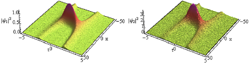
Figure 26: (Color online) The same as in Fig. 23(c,d), but in the case when strong random noise is added to the simulations. The results are reproduced from Fig. add8 .

Thus, the two-component BEC with attractive interactions in the time-dependent expulsive trap, adjusted to the integrable system based on Eqs. (120) and (136), is more long-lived, as its lifetime can be increased by means of the FR management, in comparison with the condensates in the time-independent expulsive trap, which quickly decays in the course of the evolution.

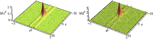
Figure 27: (Color online) The same as in Fig. 24(c,d), but in the case when strong random noise is added to the simulations. The results are reproduced from Ref. add8 .

To further confirm the stability of the exact soliton solution produced by Eqs. (120) and (136), one can add random noise to the simulations (while rigorous stability analysis for these solutions in an experimentally relevant form is not straightforward). The respective numerically simulated density profiles demonstrate, in Figs. 25-27, that the white noise does not break the stability of the evolving condensates. Additional numerical results demonstrate that the stability does not depend on the particular correlation structure of the noise (white or colored), nor on its spectral width. This conclusion further corroborates that the two-component condensate in the time-dependent expulsive HO, governed by the specially devised integrable system, is more robust in comparison with its counterpart in the time-independent trap. The above results indicate the possibility of increasing the life span of the two-component BEC with the time-modulated attractive interactions in the time-dependent HO potential. These predictions may be realized experimentally in condensates composed of ³⁹K 4.15 , ⁸⁵Rb 4.13 and ⁷Li 3.30 atoms.

V.3 Conclusion of the section

It is shown that the temporal modulation of the scattering length by means of FR can be efficiently used to design conditions under which the mean-field dynamics of two-component condensates in the time-dependent expulsive HO potential is governed by the integrable model. The solitons generated by this integrable system stay stable for a reasonably large interval of time, compared to the condensate in the time-independent expulsive HO potential. The analytical results and their stability are corroborated by comparison with numerical simulations, including the case when strong random noise is added to the simulations.

VI Soliton motion in a binary Bose-Einstein condensate

This section deals with the analytical study of dynamics of matter-wave solitons governed by an integrable system of coupled GP equations of the Manakov’s type 4.14 , modeling a two-component BEC. By means of the Darboux transform (DT), analytical solutions of these equations can be obtained for a soliton set on top of a plane-wave background. These solutions with and without the XPM interaction between the two components are considered. In the presence of XPM, the solutions exhibit properties different from those in the single-component GP, such as restriction of MI and soliton splitting.

The results presented in this section are essentially based on Ref. 5.1 .

VI.1 The model and analysis

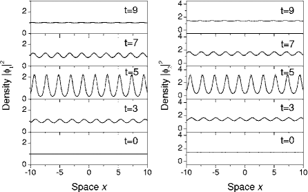
Figure 28: (Color online) A set of snapshots showing exact solution (161a) by dotted curves, and numerical results, obtained under nearly integrable condition (166), by solid curves (in fact, the dotted and solid plots completely overlap). Parameters are $\eta=0.8$, $k=-0.1$,$g=1$, $A_{1}=1$, $A_{2}=1.2$, $\theta_{10}=6$, the latter one representing amplitude (164) of the initial perturbation which triggers the onset of MI, with $\epsilon=2.4788\times 10^{-3}$ and $\varphi_{10}=0$. The results are reproduced from Ref. 5.1 .

The subject on this section is the system of coupled 1D GP equations for two-component self-attractive BEC with negative scattering lengths. In the scaled form, these equations are

$$i\frac{\partial\phi_{j}}{\partial t}=-\frac{1}{2}\frac{\partial^{2}\phi_{j}}{\partial x^{2}}-g\left(\frac{a_{ij}}{a_{12}}\left|\phi_{j}\right|^{2}+\left|\phi_{3-j}\right|^{2}\right)\phi_{j},\text{\ }j=1,2,$$ (150)

where $a_{jj}$ and $a_{12}$ are, respectively, the negative scattering lengths of intra- and inter-component atomic collisions, coordinate $x$ is measured in units of $x_{0}\sim 1~{}\mathrm{\mu}$m, $t$ in units of $mx_{0}^{2}/\hbar$, with atomic mass $m$, $\phi_{j}$ in units of $\sqrt{n_{0}}$ ($n_{0}$ is the maximum density of the initial distribution of the condensate), and the interaction constant is defined as $g=4\pi n_{0}x_{0}^{2}\left|a_{12}\right|$.

As is well known, coupled equations (150) are integrable in the Manakov’s case, with $a_{11}=a_{22}=a_{12}$ 4.14 . In this case, by means of DT, one can generate an exact two-component solution which accounts for a soliton interacting with a plane wave:

$$\phi_{j}=A_{j}\exp\left(i\varphi\right)\left(1+\frac{4i\eta G_{1}}{F}\right)+\frac{2\eta\overline{C}_{j}G_{2}}{\sqrt{g}}\exp\left(\frac{i}{2}\varphi\right),$$ (151)

where $j=1,2$, and

$$F = D\exp\theta_{1}+A^{2}D\exp\left(-\theta_{1}\right)-2iA^{2}\left(L-\overline{L}\right)\sin\varphi_{1}+C\exp\left(-\theta_{2}\right),$$ (152a)

$$G_{1} = L\exp\theta_{1}-A^{2}\overline{L}\exp\left(-\theta_{1}\right)-\left|L\right|^{2}\exp\left(-i\varphi_{1}\right)+A^{2}\exp\left(i\varphi_{1}\right),$$ (152b)

$$G_{2} = L\exp\left[-\frac{i}{2}\left(\varphi_{1}+\varphi_{2}\right)+\frac{1}{2}\left(\theta_{1}-\theta_{2}\right)\right]+A^{2}\exp\left[\frac{i}{2}\left(\varphi_{1}-\varphi_{2}\right)-\frac{1}{2}\left(\theta_{1}+\theta_{2}\right)\right];$$ (152c)

$$\theta_{1} \equiv M_{I}x+\frac{1}{2}\left[\left(\xi-k\right)M_{I}+\eta M_{R}\right]t-\theta_{10},$$ (152d)

$$\theta_{2} \equiv \eta x+\eta\xi t+\theta_{10},$$ (152e)

$$\varphi_{1} \equiv M_{R}x+\frac{1}{2}\left[\left(\xi-k\right)M_{R}-\eta M_{I}\right]t+\varphi_{10},$$ (153)

$$\varphi_{2} \equiv \xi x+\frac{1}{2}\left(\xi^{2}-\eta^{2}\right)t-\varphi_{10},$$ (154)

$$\varphi \equiv kx+\left[g\left(A_{1}^{2}+A_{2}^{2}\right)-\frac{1}{2}k^{2}\right]t;$$ (155)

$$L \equiv M_{R}+\xi+k+i\left(M_{I}+\eta\right),M\equiv\sqrt{\left(k+\xi+i\eta\right)^{2}+A^{2}}=\text{\ }M_{R}+iM_{I},$$ (156)

$$D \equiv \left|L\right|^{2}+A^{2},A\equiv\sqrt{4g\left(A_{1}^{2}+A_{2}^{2}\right)},C=\left|C_{1}\right|^{2}+\left|C_{2}\right|^{2},$$ (157)

$k$, $\theta_{10}$, $\varphi_{10}$, $A_{1,2}$ are arbitrary real constants, and $C_{1,2}$ are arbitrary complex constants subject to constraint

$$A_{1}C_{1}+A_{2}C_{2}=0.$$ (158)

In the case of zero background amplitude, $A_{1}=A_{2}=0$, solution (151) amounts to $\phi_{j}=\left[\eta\epsilon_{j}/\left(\sqrt{g}\cosh\theta\right)\right]\exp\left(-i\varphi_{2}\right)$, where $\theta=\eta\left(x+\xi\right)-\theta_{0}$, $\theta_{0}$ is an arbitrary real constant, and $\epsilon_{1,2}$ are arbitrary complex constants obeying relation $\left|\epsilon_{1}\right|^{2}+\left|\epsilon_{2}\right|^{2}=1$. The latter solution is a stable two-component soliton with velocity $V_{\text{sol}}=-\xi$, width $\eta^{-1}$, and amplitudes $A_{s1,2}=\left|\eta\epsilon_{1,2}\right|/\sqrt{g}$ which satisfy relation $A_{s1}^{2}+A_{s2}^{2}=\eta^{2}/g$. The total norm of the two-component soliton (proportional to the number of atoms in the binary condensate) is $Q\equiv Q_{1}+Q_{2}=\int_{-\infty}^{+\infty}\left(\left|\phi_{1}\right|^{2}+\left|\phi_{2}\right|^{2}\right)dx=2\left|\eta\right|/g,$ with $Q_{j}=2\left|\eta\right|\left|\epsilon_{j}\right|^{2}/g$. Further, its momentum and Hamiltonian of the system are

$$M\equiv M_{1}+M_{2}=-\frac{i}{2}\int_{-\infty}^{+\infty}\left[\left(\overline{\phi}_{1}\phi_{1,x}-\phi_{1}\overline{\phi}_{1,x}\right)+\left(\overline{\phi}_{2}\phi_{2,x}-\phi_{1}\overline{\phi}_{2,x}\right)\right]dx=V_{\text{sol}}Q$$ (159)

and

$$H\equiv\frac{1}{2}\int_{-\infty}^{+\infty}\left[\left(\left|\phi_{1,x}\right|^{2}+\left|\phi_{2,x}\right|^{2}\right)-g\left(\left|\phi_{1}\right|^{2}+\left|\phi_{2}\right|^{2}\right)^{2}\right]dx=\frac{M^{2}}{2Q}-\frac{g^{2}}{24}Q^{3}.$$ (160)

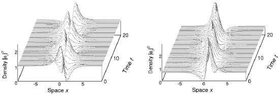
Figure 29: Spatiotemporal distribution of densities of the two components in solution (167), with phase difference $\pi$ between the components. Parameters are $k=-0.1$, $g=1$, $A_{1}=1$, $A_{2}=0.8$, $\theta_{10}=-2$, and $\varphi_{10}=0$. The results are reproduced from Ref.

On the other hand, when the soliton’s amplitudes vanish, $A_{1s,2s}=0$ (e.g., $\eta=0$), solution (151) reduces to the plane wave (alias CW), $\phi_{1,2}=A_{1}\exp\left(i\varphi\right)$, with amplitudes $A_{1,2}$, wave number $k$, and frequency $\Omega=g\left(A_{1}^{2}+A_{2}^{2}\right)-k^{2}/2$. Thus, in the general case exact solution (151) represents a two-component soliton embedded in the CW background. Condition (158) determines the XPM interaction between the two components of the plane-wave background. If $C_{1}=C_{2}=0$, the second term in solution (151) vanishes, each soliton component being embedded in its own background, see a more detailed consideration of this special case below. If $C_{1}C_{2}\neq 0$, the second term in solution (151) is different from zero, hence condition (158) implies that coefficients $C_{1}$ and $C_{2}$ depend on the CW amplitudes $A_{2}$ and $A_{1}$.

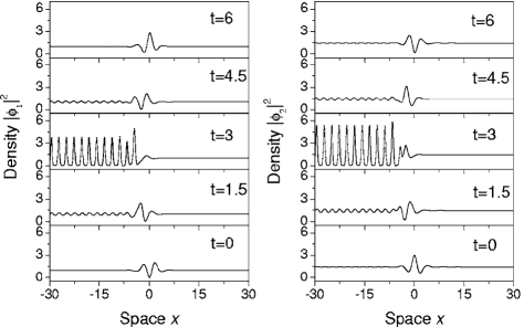
Figure 30: A set of snapshots representing exact solution (169) for $\eta=-1.5$, $k=-0.1$, $g=1$, $A_{1}=1$, $A_{2}=1.2$, $\theta_{10}=-6$, $\varphi_{10}=0$, and $\theta_{20}=-5$, $\varphi_{20}=0$. The results are reproduced from Ref. 5.1 .

To understand the behavior of solution (151), it is relevant to start with the above-mentioned case of $C_{1}=C_{2}=0$, when solution (151) simplifies to

$$\phi_{j} = A_{j}\exp\left(i\varphi\right)\left(1-2\eta W\right),$$ (161a)

$$W \equiv \frac{1}{A}\left(\frac{a\cosh\theta_{1}+\sin\varphi_{1}}{\cosh\theta_{1}+a\sin\varphi_{1}}-i\frac{b\sinh\theta_{1}+c\cos\varphi_{1}}{\cosh\theta_{1}+a\sin\varphi_{1}}\right),$$ (161b)

with $$a=-iA\left(L-\overline{L}\right)/D, b=A\left(L+\overline{L}\right)/D c=\left(A^{2}-\left|L\right|^{2}\right)/D \theta_{2} \varphi_{2} M_{I}\neq 0$$ , and . Note that expressions (161a) and (161b) do not include and , and the two components share a common shape. This solution is similar to that for the single-component BEC. As , from Eq. (161a) one can extract the total norm of the soliton component of the solution, which is defined as the norm above the CW level:

$$\int_{-\infty}^{+\infty}\left[\left(\left|\phi_{1}\right|^{2}-A_{1}\right)^{2}+\left(\left|\phi_{2}\right|^{2}-A_{2}^{2}\right)\right]dx=\frac{\eta\left(b^{2}+c^{2}\right)}{g\left|M_{I}\right|}I,$$ (162a)

$$I\equiv\int_{-\infty}^{+\infty}\frac{\eta+A\left(\cosh x\right)\sin\left(Bx+\Delta\right)}{\cosh x+a\sin\left(Bx+\Delta\right)}dx,$$ (162b)

where $$\Delta=-(1/2)\eta M_{I}\left(1+B^{2}\right)t+B\theta_{10}+\varphi_{10} B=M_{R}/M_{I} \left|\phi_{1}(\pm\infty,t)\right|^{2}=A_{1}^{2} \left|\phi_{2}(\pm\infty,t)\right|^{2}=A_{2}^{2} \Delta$$ and . In deriving the above expression, relations and for asymptotic values of the fields are used. It can be verified that integral (162b) does not depend on , hence the soliton’s total norm is a conserved quantity.

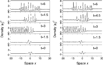
Figure 31: The same as in Fig. 30, but obtained from a numerical solution of Eqs. (150) with the nonlinearity constants taken as per Eq. (166). Other parameters are identical to those in Fig. 30. The results are reproduced from Ref. 5.1 .

When $M_{I}=0$, the soliton’s velocity vanishes, i.e., the CW background completely traps the soliton 5.1 . Setting, in particular, $\xi=-k$ and $A^{2}>\eta^{2}$ yields $M_{I}=0$, and $W$ in solution (161a) becomes

$$W=\frac{1}{A}\frac{\eta\cosh\theta_{1}+A\sin\varphi_{1}-iM_{R}\sinh\theta_{1}}{A\cosh\theta_{1}+\eta\sin\varphi_{1}},$$ (163)

with $\theta_{1}\equiv(1/2)\eta M_{R}t-\theta_{10}$ and $\varphi_{1}\equiv M_{R}\left(x-kt\right)+\varphi_{10}$, where $M_{R}=\sqrt{A^{2}-\eta^{2}},$ and $\theta_{10}$ and $\varphi_{10}$ are arbitrary real constants. Expression (163) is periodic in $x$, with period $\Lambda=2\pi/M_{R}$, and aperiodic in $t$. To better understand the MI development provided by this solution, one may assume that

$$\epsilon=\exp\left(-\theta_{10}\right)$$ (164)

is small (it then plays the role of a small amplitude of the initial perturbation that triggers the onset of the MI), and linearize the initial form of solution (161a) at $t=0$ with respect to $\epsilon$, taking Eq. (163) into account. This yields

$$\phi_{j}(x,0)\approx A_{j}\exp\left(i\varphi\right)\left[\rho-\epsilon\chi\sin\left(M_{R}x+\varphi_{10}\right)\right],$$ (165)

where $\rho\equiv\left(A^{2}-2\eta^{2}-2i\eta M_{R}\right)/A^{2}$ with $\left|\rho\right|^{2}=1$, $\chi\equiv 4\eta M_{R}\left(M_{R}-i\eta\right)/A^{3}$. Direct numerical simulations of the underlying equations (150) demonstrate that the evolution of initial configuration (165), which is a plane wave with a small modulational perturbation added to it, indeed closely follows the exact solution provided by Eqs. (161a) and (163) 5.1 .

VI.2 Results

The above results were obtained under the Manakov integrability conditions $a_{11}=a_{22}=a_{12}$, which may not be exactly satisfied in reality. However, the actual difference of the scattering lengths in a BEC mixture of two different hyperfine states of the same atomic species is very small, therefore the Manakov’s system may be used as a good approximation. For instance, taking

$$a_{11}=-1.03,\text{ }a_{12}=-1,\text{ }a_{22}=-0.97,$$ (166)

numerical solution of Eqs. (150) yields the picture of the MI development shown in Fig. 28. Comparing it with the exact solution obtained for $a_{11}=a_{22}=a_{12}$ demonstrates that the two solutions are virtually indistinguishable.

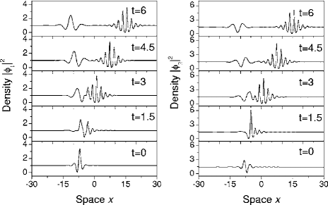
Figure 32: A set of snapshots of the general-form analytical solution (151). Parameters are $\eta=1.5$, $\xi=-0.4$, $k=-0.5$, $g=1$, $A_{1}=1$, $A_{2}=1.2$, $10=5$, $10=0$, $C_{1}=1$, and $C_{2}$ is determined by constraint (158). The results are reproduced from Ref. 5.1 .

The consideration of solution (151) in a more general situation, with nonzero coefficients $C_{1,2}$ and $A_{1,2}$, subject to condition (158), make it possible to explicitly consider effects of the XPM interaction between the plane waves in the two-component BEC. In this case, to satisfy condition (158), one sets $C_{1}=4\sqrt{g}A_{2}C$ and $C_{2}=-4\sqrt{g}A_{1}C$, where $C$ is an arbitrary complex constant. Further, one fixes $\xi=-k$ in solution (151) to analyze two following representative situations in detail.

(i) Setting $A^{2}=\eta^{2}$, i.e., $4\left(A_{1}^{2}+A_{2}^{2}\right)=A_{s1}^{2}+A_{s2}^{2}$, solution (151) can be written as

$$\phi_{j}=-\exp\left(i\varphi\right)\left[A_{j}\tanh\left(\theta_{2}/2\right)+(-1)^{j}\sqrt{2}A_{3-j}\cosh^{-1}\left(\theta_{2}/2\right)\exp\left(i\varphi_{3}\right)\right],$$ (167)

where $\theta_{2}\equiv\eta\left(x-kt\right)+\theta_{10},$ $\varphi\equiv kx+\left(\eta^{2}/4-k^{2}/2\right)t,$ $\varphi_{3}\equiv\eta^{2}t/8+\varphi_{10}$, and $\theta_{10}$ and $\varphi_{10}$ are arbitrary real constants. The density distribution corresponding to this solution is $\left|\phi_{1}\right|^{2}+\left|\phi_{2}\right|^{2}=$ $\left(A_{2}^{2}+A_{1}^{2}\right)\left[1+\mathrm{sech}^{2}\left(\theta_{2}/2\right)\right]$, see Fig. 29. Solution (167) may be regarded as a superposition of bright and dark solitons, produced by the action of XPM. In particular, the solution with $A_{1}=0$ or $A_{2}=0$ is a complex consisting of bright and dark solitons in the first and second species, or vice versa. From the imposed condition $A^{2}=$ $\eta^{2}$, it follows that $\left|\eta\right|=\sqrt{4g\left(A_{1}^{2}+A_{2}^{2}\right)}$, showing that the width of the soliton is controlled by the amplitude of the CW background. In Fig. 29 one observes a shift of the soliton’s peak due to the action of XPM.

(ii) In the case when $A^{2}>\eta^{2}$, i.e.,

$$4\left(A_{1}^{2}+A_{2}^{2}\right)>A_{s1}^{2}+A_{s2}^{2},$$ (168)

solution (151) can be written as

$$\phi_{j}=A_{j}\exp\left(i\varphi\right)\left(1-2\eta W_{1}\right)-\left(-1\right)^{j}2\eta A_{3-j}W_{2},$$ (169)

$$W_{1} = \frac{1}{A}\frac{\eta\cosh\theta_{1}+A\sin\varphi_{1}-iM_{R}\sinh\theta_{1}}{A\cosh\theta_{1}+\eta\sin\varphi_{1}+A\exp\left(-\theta_{2}\right)},$$ (170a)

$$W_{2} = \frac{1}{A}\frac{\left(M_{R}+i\eta\right)\exp\left[\left(-i\varphi_{1}+\theta_{1}\right)/2\right]+A\exp\left[\left(i\varphi_{1}-\theta_{1}\right)\right]}{A\cosh\theta_{1}+\eta\sin\varphi_{1}+A\exp\left(-\theta_{2}\right)}$$ (170b)

$$\times\exp\left[\frac{-\theta_{2}+i\left(\varphi-\varphi_{2}\right)}{2}\right],$$

with $$\theta_{1}\equiv\left(\eta/2\right)M_{R}t-\theta_{10} \theta_{2}\equiv x-kt+\theta_{20} \varphi_{1}\equiv M_{R}\left(x-kt\right) + \varphi_{10} \varphi_{2}\equiv-kx+\frac{1}{2}\left(k^{2}-\eta^{2}\right)t-\varphi_{20} M_{R}=\sqrt{A^{2}-\eta^{2}} \theta_{10} \theta_{20} \varphi_{10} \varphi_{20} W_{2}\rightarrow 0 \theta_{2}\rightarrow\pm\infty W_{1}\rightarrow W \theta_{2}\rightarrow+\infty W_{1}\rightarrow 0 \theta_{2}\rightarrow-\infty \theta_{2}\rightarrow-\infty a_{11} a_{12} a_{22} a_{11}=a_{12}=a_{22}$$, , , , and , while , , , and are arbitrary real constants. From expressions (170a) and (170b) one can see that at , and at , at . Thus, taking into regard the form of solution (161a) and expression (163), one concludes that solution (169) describes partial MI, because the growth of the instability is restrained in the limit of , as illustrated by Fig. 30. However, if the nonlinearity constants , , and slightly deviate from the integrable case , a numerically found counterpart of solution (169) is conspicuously different from it, see Fig. 31.

Finally, one can consider solution (151) in the general case. From expressions (152d) and (152e) one sees that the solution contains terms with different velocities, $V_{1}=-(1/2)\left[\left(\xi-k\right)+\eta M_{R}/M_{I}\right]$ and $V_{2}=-\xi$, which leads to splitting of the soliton part of the solution on top of the CW background in two wave packets, high- and low-frequency ones, as shown in Fig. 32. Further, in Fig. 33 this exact analytical solution, obtained in the integrable case with $a_{11}=a_{12}=a_{22}=1$, is compared to a numerically found one, produced by the generic nonintegrable version of Eqs. (150), with the normalized scattering lengths chosen as in Eq. (166). Figure 33 demonstrates that the soliton part of the numerically found solution, built on top of the CW background, also splits in two packets, stable high-frequency and unstable low-frequency ones.

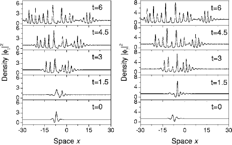
Figure 33: The same as in Fig. 32, but for a numerically found solution of Eqs. (150) with $a_{11}=-1.03$, $a_{12}=-1$, $a_{22}=-0.97$. Other parameters are identical to those in Fig. 32. The results are reproduced from Ref. 5.1 .

VI.3 Conclusion of the section

Exact solutions are presented for coupled GP equations describing binary BEC, in the form of a soliton placed on top of a CW (plane-wave) background. It is shown that, when the intensity of the CW background exceeds a quarter of the soliton’s peak intensity, which is expressed by condition (168), the exact solution, produced by the Manakov system, describes development of MI, which can be used in physical applications to generate a soliton train. This wave complex can be generated, as a robust one, even if parameters of the coupled equations do not exactly satisfy the Manakov’s integrability condition. The XPM interaction in the CW background of the two-components system has been considered too. It was shown that the interaction between two CW amplitudes gives rise to a phase difference between the components, and, in the most general case, it causes splitting of the soliton and formation of a complex pattern. In particular, under condition (168) as mentioned above, the XPM interaction between the two plane waves helps to effectively restrain the MI.

Note that the coupled underlying equations (150) are also integrable in the case of $g<0$ and $a_{11}=a_{22}=a_{12}$ (a binary self-repulsive condensate), and also, with either sign of $g$, for $a_{11}=a_{22}=-a_{12}$ 5.2 , which corresponds to a mixture of two self-repulsive condensates that attract each other, or two self-attractive ones which repel each other. In the former case, when single-component bright solitons are impossible due to the intraspecies repulsion, the so-called symbiotic solitons exist and are stable, being supported by the inter-species attraction 5.3 ; symbio2 . However, direct attempts to construct bound states of plane waves and solitons by means of DT lead to singular solutions in these cases 5.1 .

VII Dynamics of matter-wave solitons in spinor BEC

This section addresses the dynamics of matter-wave solitons in the general nonintegrable model of a three-component spinor BEC, based on a system of three nonlinearly coupled GP equation. First, one-, two-, and three-component solitons of the polar and ferromagnetic (FM) types are produced. Next, BdG equations for small perturbations are used to study the stability of the solitons by means of direct simulations and, in a part, analytically. Global stability of the solitons is considered by means of comparison of energy for different states. As the main result, ground-state and metastable soliton states of the FM and polar types are identified. Considering the special case of the integrable version of the system, DT is applied to find analytical solutions that display full nonlinear evolution of MI of CW states, seeded by a small spatially periodic perturbation. Also, it is demonstrated that solitons of both the polar and FM types, found in the integrable system, are robust against random changes of the nonlinearity coefficient in time (i.e., random deviations form the integrability). The latter result demonstrates structural stability of the solitons.

The results collected in this section are essentially based on Ref. 6.1 .

VII.1 Formulation of the model

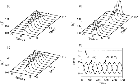
Figure 34: The evolution of the single-component polar soliton (182) with a small random perturbation added, at $t=0$, to the $\phi_{+1}$ and $\phi_{-1}$ components. Parameters are $\nu=1$, $a=-0.5$, and $\mu=-1$. The results are reproduced from Ref. 6.1

The object considered here is an effectively 1D BEC loaded in a cigar-shaped trap, which is elongated in $x$ and tightly confined in the transverse plane $\left(y,z\right)$ 3.5 . In the mean-field approximation, atoms in the hyperfine state with atomic spin $F=1$ are described by a 1D three-component wave function, $\mathbf{\Phi}(x,t)=\left[\Phi_{+1}(x,t),\Phi_{0}(x,t),\Phi_{-1}(x,t)\right]^{\mathrm{T}}$, with the components corresponding to the three values of the vertical spin projection, $m_{F}=+1,$ $0,$ $-1$ Ho . The wave functions obey the corresponding three-component system of GP equations Ho ; Ueda1 ; Ueda2 :

$$i\hslash\frac{\partial\Phi_{\pm 1}}{\partial t} = -\frac{\hslash^{2}}{2m}\frac{\partial^{2}\Phi_{\pm 1}}{\partial x^{2}}+\left(c_{0}+c_{2}\right)\left(\left|\Phi_{\pm 1}\right|^{2}+\left|\Phi_{0}\right|^{2}\right)\Phi_{\pm 1}+\left(c_{0}-c_{2}\right)$$

$$\times\left|\Phi_{\mp 1}\right|^{2}\Phi_{\pm 1}+c_{2}\Phi_{\mp 1}^{\ast}\Phi_{0}^{2},$$

$$i\hslash\frac{\partial\Phi_{0}}{\partial t} = -\frac{\hslash^{2}}{2m}\frac{\partial^{2}\Phi_{0}}{\partial x^{2}}+\left(c_{0}+c_{2}\right)\left(\left|\Phi_{+1}\right|^{2}+\left|\Phi_{-1}\right|^{2}\right)\Phi_{0}$$

$$+c_{0}\left|\Phi_{0}\right|^{2}\Phi_{0}+2c_{2}\Phi_{+1}\Phi_{-1}\Phi_{0}^{\ast},$$

where $c_{0}=\left(g_{0}+2g_{2}\right)/3$ and $c_{2}=\left(g_{2}-g_{0}\right)/3$ denote, respectively, effective constants of the spin-independent and spin-exchange interactions 6.1 ; 6.2 . In terms of similar optics models, $c_{2}$ is the coefficient of the four-wave mixing, while $c_{0}\pm c_{2}$ account for the SPM and XPM interactions. Here $g_{f}$ $=4\hslash^{2}a_{f}/\left[ma_{\bot}^{2}\left(1-ca_{f}/a_{\bot}\right)\right]$ , with $f=0,2$, are effective 1D coupling constants, $a_{f}$ is the s-wave scattering length in the channel with total hyperfine spin $f$, $a_{\bot}$ is the size of the transverse ground state, $m$ is the atomic mass, and $c=-\zeta\left(1/2\right)\approx 1.46$. Redefining the wave function as $\mathbf{\Phi}\rightarrow\left(\phi_{+1},\sqrt{2}\phi_{0},\phi_{-1}\right)^{\mathrm{T}}$ and measuring time and length in units of $\hslash/\left|c_{0}\right|$ and $\sqrt{\hslash^{2}/2m\left|c_{0}\right|}$, respectively, one casts system (VII.1) in the scaled form:

$$i\frac{\partial\phi_{\pm 1}}{\partial t} = -\frac{\partial^{2}\phi_{\pm 1}}{\partial x^{2}}-\left(\nu+a\right)\left(\left|\phi_{\pm 1}\right|^{2}+2\left|\phi_{0}\right|^{2}\right)\phi_{\pm 1}-\left(\nu-a\right)\left|\phi_{\mp 1}\right|_{\pm 1}^{2}\phi_{\pm 1}$$ (172)

$$-2a\phi_{\mp 1}^{\ast}\phi_{0}^{2},$$

$$i\frac{\partial\phi_{0}}{\partial t} = -\frac{\partial^{2}\phi_{0}}{\partial x^{2}}-2\nu\left|\phi_{0}\right|^{2}\phi_{0}-\left(\nu+a\right)\left(\left|\phi_{+1}\right|^{2}+\left|\phi_{-1}\right|^{2}\right)\phi_{0}-2a\phi_{+1}\phi_{-1}\phi_{0}^{\ast},$$

where $\nu\equiv-$sgn$\left(c_{0}\right)$ and $a\equiv-c_{2}/c_{0}$.

System (172) can be derived from the Hamiltonian,

$$H = \int_{-\infty}^{+\infty}dx\left\{\left|\frac{\partial\phi_{+1}}{\partial x}\right|^{2}+\left|\frac{\partial\phi_{-1}}{\partial x}\right|^{2}-\frac{1}{2}\left(\nu+a\right)\left(\left|\phi_{+1}\right|^{4}+\left|\phi_{-1}\right|^{4}\right)\right.$$

$$-\left(\nu-a\right)\left|\phi_{+1}\right|^{2}\left|\phi_{-1}\right|^{2}+2\left[\left|\frac{\partial\phi_{0}}{\partial x}\right|^{2}-\nu\left|\phi_{0}\right|^{4}-\left(\nu+a\right)\right.$$

$$\left.\left.\times\left(\left|\phi_{+1}\right|^{2}+\left|\phi_{-1}\right|^{2}\right)\left|\phi_{0}\right|^{2}-a\left(\phi_{+1}^{\ast}\phi_{-1}^{\ast}\phi_{0}^{2}+\phi_{+1}\phi_{-1}\left(\phi_{0}^{\ast}\right)^{2}\right)\right]\right\},$$

which is a dynamical invariant of the model ($dH/dt=0$). Moreover, system (172) conserve the momentum, i.e.,

$$P=i\int_{-\infty}^{+\infty}\left(\phi_{+1}^{\ast}\frac{\partial\phi_{+1}}{\partial x}+\phi_{-1}^{\ast}\frac{\partial\phi_{-1}}{\partial x}+2\phi_{0}^{2}\frac{\partial\phi_{0}}{\partial x}\right)dx,$$ (174)

the solution’s norm, proportional to total number of atoms,

$$N=\int_{-\infty}^{+\infty}\left[\left|\phi_{+1}(x,t)\right|^{2}+\left|\phi_{-1}(x,t)\right|^{2}+2\left|\phi_{0}(x,t)\right|^{2}\right]dx,$$ (175)

and the total magnetization,

$$\mathbf{M}=\int_{-\infty}^{+\infty}\left[\left|\phi_{+1}(x,t)\right|^{2}-\left|\phi_{-1}(x,t)\right|^{2}\right]dx.$$ (176)

These conservation laws are generated by symmetries of the system of GP equations (172). In particular, the conservation of the magnetization is related to the invariance of the system with respect to rotation of the atomic spin.

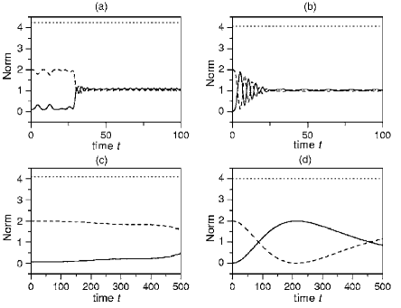
Figure 35: Solid, dashed, and dotted curves show, respectively, the evolution of norms $N_{0}$, $N_{\pm}$ of the $\phi_{0}$ and $\phi_{\pm 1}$ components, and total norm $N$ (see Eqs. (186) and (175)) in the two-component polar soliton (187) perturbed by a small random perturbation introduced in the $\phi_{0}$ component. Parameters are $\nu=1$ and $\mu=-1$ and (a) $a=1.5$ for $\phi_{+1}\phi_{-1}^{\ast}<0$; (b) $a=1.5$ for $\phi_{+1}\phi_{-1}^{\ast}>0$; (c) $a=-1.5$ for $\phi_{+1}\phi_{-1}^{\ast}<0$; (d) $a=-1.5$ for $\phi_{+1}\phi_{-1}^{\ast}>0$. The results are reproduced from Ref. 6.1 .

An obvious reduction of system (172) can be obtained by setting $\phi_{0}=0$. In this case, the model reduces to a system of two equations which are tantamount to those describing light transmission in bimodal nonlinear optical fibers, with the two modes representing either different wavelengths or two orthogonal polarizations 6.1 :

$$i\frac{\partial\phi_{\pm 1}}{\partial t}=-\frac{\partial^{2}\phi_{\pm 1}}{\partial x^{2}}-\left(\nu+a\right)\left|\phi_{\pm 1}\right|^{2}\phi_{\pm 1}-\left(\nu-a\right)\left|\phi_{\mp 1}\right|^{2}\phi_{\pm 1}.$$ (177)

In particular, the case of two linear polarizations in the birefringent fiber corresponds to $\left(\nu-a\right)/\left(\nu+a\right)$ $=2/3$, i.e., $a=\nu/5$ and two different carrier waves of circular polarizations correspond to $\left(\nu-a\right)/\left(\nu+a\right)=2$, i.e., $a=-\nu/3$. The two nonlinear terms in system (177) account for, respectively, the SPM and XPM interactions of the two waves. The MI of CW (uniform) states in the system of two XPM-coupled equations (177) has been studied in detail 6.3 . If the nonlinearity in system (177) is self-defocusing, i.e., $\nu=-1$ and $1\pm a>0$ (in other words, $\left|a\right|<$ $1$), the single NLS equation would of course show no MI, but the XPM-coupled system of NLS equations (177) gives rise to MI, provided that the XPM interaction is stronger than SPM, i.e., $0<a<1$ Agrawal-XPM .

VII.2 Analytical one-, two-, and three-component soliton solutions

As follows from the above derivation, the special case of the integrable model (with $a=\nu=1$ Wadati ) is physically possible, corresponding to $c_{2}=c_{0}$ or, equivalently, $2g_{0}=-g_{2}>0$. The condition $2g_{0}=-g_{2}>0$ can be satisfied by imposing condition

$$a_{\bot}=3ca_{0}a_{2}/\left(2a_{0}+a_{2}\right)$$ (178)

on the scattering lengths, provided that $a_{0}a_{2}\left(a_{2}-a_{0}\right)>0$ holds.

However, it is also possible to find simple exact soliton solutions of both polar and FM types in the general (non-integrable) case $a\neq\nu$. Several soliton species and results for their stability are presented below, following Ref. 6.1 .

VII.2.1 Single-component FM solitons

A one-component FM soliton is given by a straightforward single-component solution (assuming $a+\nu>0$):

$$\phi_{-1}=\phi_{0}=0,\text{ }\phi_{+1}=\sqrt{-\frac{2\mu}{\nu+1}}\frac{\exp\left(-i\mu t\right)}{\cosh\left(\sqrt{-\mu}x\right)},$$ (179)

where chemical potential $\mu<0$ is an intrinsic parameter of the soliton family. While expression (179) corresponds to the zero-velocity soliton, moving ones can be generated from it in an obvious way by means of the Galilean transformation. Note that condition $a+\nu>0$ implies $a>1$ or $a>-1$ in the cases of the, respectively, repulsive ($\nu=-1$) or attractive ($\nu=+1$) spin-independent interaction. Norm (175) and energy (VII.1) of this soliton are

$$N=\frac{4\sqrt{-\mu}}{\nu+a}\text{, }H=-\frac{\left(\nu+a\right)^{2}}{48}N^{3}.$$ (180)

Soliton (179) is stable against small perturbations, as the linearization of system (172) about this solution demonstrates that the BdG equations for small perturbations are decoupled. Then, because the standard soliton of the single NLS equation is always stable, solution (179) cannot be unstable against small perturbations of $\phi_{+1}$. Further, the decoupled BdG equations for small perturbations $\phi_{-1}$ and $\phi_{0}$ of the other fields are

$$\frac{\partial\phi_{-1}}{\partial t} = -\frac{\partial^{2}\phi_{-1}}{\partial x^{2}}-\left(\nu-a\right)\left|\phi_{+1}\right|^{2}\phi_{-1},$$ (181a)

$$\frac{\partial\phi_{0}}{\partial t} = -\frac{\partial^{2}\phi_{0}}{\partial x^{2}}-\left(\nu+a\right)\left|\phi_{+1}\right|^{2}\phi_{0},$$ (181b)

and it is well known that such linear equations, with $$\left|\phi_{+1}\right|^{2}$$ corresponding to the unperturbed soliton (179), give rise to no instabilities either.

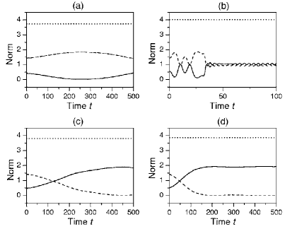
Figure 36: The evolution of the three-component polar soliton (LABEL:eq_7.20) under the action of a small random perturbation initially added to the $\phi_{0}$ component. Parameters are $\nu=1$, $\mu=-0.8$, and $\epsilon=2/\sqrt{5}$ and (a) $a=0.5$; (b) $a=1.5$; (c) $a=-0.5$; (d) $a=-1.5$. The meaning of the solid, dashed, and dotted curves is the same as in Fig. 35. The results are reproduced from Ref. 6.1 .

VII.2.2 Single-component polar solitons

The simplest polar soliton, which has only the $\phi_{0}$ component different from zero, can be found for $\nu=+1$,

$$\phi_{0}(x,t)=\sqrt{-\mu}\frac{\exp\left(-i\mu t\right)}{\cosh\left(\sqrt{-\mu}x\right)},~{}\phi_{\pm 1}(x,t)=0.$$ (182)

The stability problem for this soliton is more involved, as the unperturbed field $\phi_{0}$ gives rise to a coupled system of BdG equations for infinitesimal perturbations $\phi_{\pm 1}$ of the other fields:

$$\left(i\frac{\partial}{\partial t}+\mu\right)\chi_{\pm 1}=-\frac{\partial^{2}\chi_{\pm 1}}{\partial x^{2}}+\frac{2\mu}{\cosh^{2}\left(\sqrt{-\mu}x\right)}\left[\left(1+a\right)\chi_{\pm 1}+a\chi_{\mp 1}^{\ast}\right],$$ (183)

where we have substituted $\nu=+1$ and redefined the perturbation,

$$\phi_{\pm 1}(x,t)\equiv\chi_{\pm 1}(x,t)\exp\left(-i\mu t\right).$$ (184)

The last term in system (183) gives rise to parametric gain, which may be a source of instability. This instability can be easily understood in qualitative terms if one replaces system (183) by simplified equations, which disregard the $x$ dependence, and replace the wave form $\mathrm{sech}^{2}\left(\sqrt{-\mu}x\right)$ by its value at the soliton’s center, $x=0$:

$$i\frac{d\chi_{\pm 1}}{dt}=\mu\left[\left(1+2a\right)\chi_{\pm 1}+2a\chi_{\mp 1}^{\ast}\right].$$ (185)

An elementary consideration shows that the zero solution of linear equations (185) is unstable through a double eigenvalue in the region of $a<-1/4$.

The stability of the single-component polar soliton (182) was checked by means of direct simulations of Eqs. (172), adding a small random perturbation in components $\phi_{+1}$ and $\phi_{-1}$, the value of the perturbation being distributed uniformly between $0$ and $0.03$ (the same random perturbation is used in simulations of the stability of other solitons; see below). The result is that the soliton (182) is, indeed, always unstable, as shown in Fig. 34. In particular, panel (d) in the figure displays the time evolution of

$$N_{0}=\int_{-\infty}^{+\infty}\left|\phi_{0}(x,t)\right|^{2}dx,\text{ \ }N_{\pm 1}=\int_{-\infty}^{+\infty}\left|\phi_{\pm 1}(x,t)\right|^{2}dx.$$ (186)

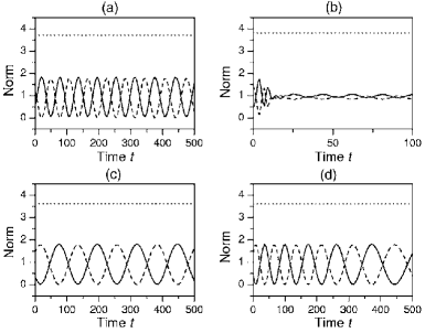
Figure 37: The same as in Fig. 35, but for the three-component polar soliton (LABEL:eq_7.21). Parameters are $\nu=1$, $\mu=-0.8$, $\epsilon=2/\sqrt{5}$, and $a=0.5$ in (a), $a=1.5$ in (b), $a=-0.5$ in (c), and $a=-1.5$ in (d). The meaning of the solid, dashed, and dotted curves is the same as in Figs. 35 and 36. The results are reproduced from Ref. 6.1 .

VII.2.3 Two-component polar solitons

In the same case as considered above, $\nu=+1$, a two-component polar soliton can be easily found too:

$$\phi_{0}(x,t)=0,\text{ }\phi_{+1}(x,t)=\pm\phi_{-1}(x,t)=\sqrt{-\mu}\frac{\exp\left(-i\mu t\right)}{\cosh\left(\sqrt{-\mu}x\right)}.$$ (187)

In this case, instability is possible due to the parametric gain revealed by the BdG equations for small perturbations. Indeed, the corresponding equation for the perturbation in the $\phi_{0}$ component decouples from the other equations and takes the form of

$$\left(i\frac{\partial}{\partial t}+\mu\right)\chi_{0}=-\frac{\partial^{2}\chi_{0}}{\partial x^{2}}+\frac{2\mu}{\cosh^{2}\left(\sqrt{-\mu}x\right)}\left[\left(1+a\right)\chi_{0}+a\chi_{0}^{\ast}\right],$$ (188)

where the perturbation was redefined the same way as in Eq. (184), $\phi_{0}(x,t)\equiv\chi_{0}(x,t)\exp\left(-i\mu t\right)$. Similar to the case of Eq. (183), the origin of the instability may be understood, replacing Eq. (188) by its simplified version that disregards the $x$ dependence, replacing the wave form $\mathrm{sech}^{2}\left(\sqrt{-\mu}x\right)$ by its value at the central point of the soliton, $x=0$:

$$i\frac{d\chi_{0}}{dt}=\mu\left[\left(1+2a\right)\chi_{0}\pm 2a\chi_{0}^{\ast}\right].$$ (189)

Elementary consideration demonstrates that the zero solution of Eq. (189) (for either sign $\pm$) is unstable in exactly the same region as in the case of system (185), viz., $a<-1/4$. While simplified equation (189) illustrates the qualitative mechanism of the parametric instability, the actual stability border may be different from $a=-1/4$. The stability of the soliton (187) was tested by direct simulations of Eqs. (172) with a small uniformly distributed random perturbation added to the $\phi_{0}$ component. The result shows that the soliton is unstable in the region of $\left|a\right|\geq 1$, as shown in Fig. 35, and it is stable at $\left|a\right|<1$ (not shown here).

The change of the stability of this soliton at $a=+1$ can be explained analytically. Indeed, splitting the perturbation into real and imaginary parts, $\chi_{0}\left(x,t\right)\equiv$ $\chi\left({}_{1}x,t\right)$ $+i\chi_{2}\left(x,t\right)$, and looking for a perturbation eigenmode as $\chi_{1,2}\left(x,t\right)=\exp\left(\sigma t\right)U_{1,2}(x)$ with instability growth rate $\sigma$, one arrives at a system of real equations,

$$-\sigma U_{2} = \left(-\frac{d^{2}}{dx^{2}}-\mu+\frac{2\mu\left(1+2a\right)}{\cosh^{2}\left(\sqrt{-\mu}x\right)}\right)U_{1},$$

$$-\sigma U_{1} = \left(-\frac{d^{2}}{dx^{2}}-\mu+\frac{2\mu}{\cosh^{2}\left(\sqrt{-\mu}x\right)}\right)U_{2}.$$

The simplest possibility for the onset of instability of the soliton is the passage of eigenvalue $\sigma$ through zero. At $\sigma=0$, system (LABEL:eq_7.19) decouples, making each equation explicitly solvable and producing the zero eigenvalue at $a=a_{n}\equiv n\left(n+3\right)/4$, $n=0,$ $1,$ $2,...$ . The vanishing of $\sigma$ at $a_{0}=0$ corresponds not to destabilization of the soliton, but to the fact that system (LABEL:eq_7.19) becomes symmetric at this point, while the zero crossings at other points indeed imply stability changes. In particular, the critical point $a_{1}=1$ explains the destabilization of soliton (187) at $a=1$ as observed in the simulations, the corresponding eigenfunctions being

$$U_{1}(x)=\frac{\sinh\left(\sqrt{-\mu}x\right)}{\cosh^{2}\left(\sqrt{-\mu}x\right)},U_{2}(x)=\frac{1}{\cosh\left(\sqrt{-\mu}x\right)}.$$ (191)

Critical points corresponding to $n>1$ imply additional destabilizations through the emergence of new unstable eigenmodes of the already unstable soliton. On the other hand, the destabilization of the soliton at $a=-1$, also observed in the simulations, may be explained by a bifurcation which changes a pair of eigenvalues $\sigma$ from purely imaginary to complex ones, developing an unstable positive real part.

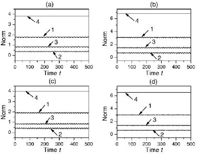
Figure 38: The evolution of the three-component polar soliton (LABEL:eq_7.22) with initially added random perturbations. Parameters are $\nu=1$, $\mu_{+1}=-1.21$, $\mu_{-1}=-0.25$, and $a=0.5$ in (a,c) or $a=-0.5$ in (b,d). In cases (a) and (b), the random perturbation was added to the $\phi_{0}$ component, and in cases (c) and (d) it was added to components $\phi_{\pm 1}$. The curves labelled by $1$, $2$, $3$, and $4$ represent, respectively, the evolution of norms $N_{+1}$, $N_{-1}$, $N_{0}$, and $N$ defined as per Eqs. (186) and (175). The results are reproduced from Ref. 6.1 .

VII.2.4 Three-component polar solitons

In the case of $\nu=+1$, three-component solitons of the polar type can be also found. One of them is

$$\phi_{0} = \sqrt{1-\epsilon^{2}}\sqrt{-\mu}\frac{\exp\left(-i\mu t\right)}{\cosh\left(\sqrt{-\mu}x\right)},$$

$$\phi_{+1} = -\phi_{-1}=\pm\epsilon\sqrt{-\mu}\frac{\exp\left(-i\mu t\right)}{\cosh\left(\sqrt{-\mu}x\right)},$$

where $\epsilon$ is an arbitrary parameter taking values $-1<\epsilon<+1$, and the opposite signs of $\phi_{+1}$ and $\phi_{-1}$ is an essential ingredient of the solution. As well as the one- and two-component polar solitons displayed above, see Eqs. (187) and (191), the solution does not explicitly depend on parameter $a$ in Eq. (172).

There is another three-component polar solution similar to the above one, i.e., containing an arbitrary parameter and independent of $a$, but with identical signs of the $\phi_{\pm 1}$ components and a phase shift of $\pi/2$ in the $\phi_{0}$ component. This solution is

$$\phi_{0} = i\sqrt{1-\epsilon^{2}}\sqrt{-\mu}\frac{\exp\left(-i\mu t\right)}{\cosh\left(\sqrt{-\mu}x\right)},$$

$$\phi_{+1} = \phi_{-1}=\pm\epsilon\sqrt{-\mu}\frac{\exp\left(-i\mu t\right)}{\cosh\left(\sqrt{-\mu}x\right)}.$$

Furthermore, there is a species of three-component polar solitons that explicitly depends on $a$:

$$\phi_{0} = i\left(\mu_{+1}\mu_{-1}\right)^{1/4}\frac{\exp\left(-i\mu t\right)}{\cosh\left(\sqrt{-\mu}x\right)},$$

$$\phi_{\pm 1} = \sqrt{-\mu_{\pm 1}}\frac{\exp\left(-i\mu t\right)}{\cosh\left(\sqrt{-\mu}x\right)},$$

where $\mu_{\pm 1}$ are two arbitrary negative parameters, and the chemical potential is $\mu=-\left(\nu+a\right)\left(\sqrt{-\mu_{+1}}+\sqrt{-\mu_{-1}}\right)^{2}/2$, which implies condition $\nu+a>0$ (note that this solution admits $\nu=-1$, i.e., repulsive spin-independent interaction). Thus, each species of the three-component polar soliton contains two arbitrary parameters: either $\mu$ and $\epsilon$ in solutions (LABEL:eq_7.20) and (LABEL:eq_7.21), or $\mu_{\pm 1}$ in solution (LABEL:eq_7.22).

The stability of all the species of these solitons was tested in direct simulations 6.1 . In the case of solutions (LABEL:eq_7.20) and (LABEL:eq_7.21), it was enough to seed a small random perturbation only in the $\phi_{0}$ component, to observe that both these types are unstable, as shown in Figs. 36 and 37.

On the contrary, the three-component polar soliton (LABEL:eq_7.22) is completely stable. This point was checked in detail by seeding small random perturbations in all the components. The result, illustrated by Fig. 38, is that the perturbation induces only small oscillations of the amplitudes of each component of the soliton.

VII.2.5 Multistability of the solitons

The above results demonstrate remarkable multistability in the system, as the FM soliton (179), two-component polar solitons (187) in the regions of $-1<a<+1$ , and the three-component one (LABEL:eq_7.22) may all be stable in the same parameter region. Then, to identify which solitons are “more stable” and “less stable,” one may fix norm (175) and compare respective values of the Hamiltonian (VII.1) for these solutions, as the ground-state solution should correspond to a minimum of $H$ at given $N$.

The substitution of the solutions in Eq. (VII.1) reveals another remarkable fact: all the solutions which do not explicitly depend on $a$, i.e., the one-, two-, and three-component polar solitons (182), (187), (LABEL:eq_7.20), and (LABEL:eq_7.21), produce identical relations between $N$, $\mu$, and $H$:

$$N=4\sqrt{-\mu},\text{ }H=-\frac{1}{48}N^{3}.$$ (195)

The $N(\mu)$ and $H(N)$ relations are different for the single-component FM soliton (179), see Eq. (180). Finally, for the stable three-component polar soliton (LABEL:eq_7.22), the relations between $\mu$, $N$, and $H$ take exactly the same form as Eq. (180) for the FM soliton.

The comparison of expressions (195) and (180) leads to a simple conclusion: the one-component FM soliton (179) and the stable three-component polar one (LABEL:eq_7.22) simultaneously provide the minimum of energy in the case of $\nu=+1$ and $a>0$, when both the spin-independent and spin-exchange interactions between atoms are attractive. In these cases, each of these two species (179) and (LABEL:eq_7.22) plays the role of the ground state in its own class of the solitons, viz., FM and polar ones, respectively. Simultaneously, the two-component soliton (187) is also stable in the region of $0<a<1$, as shown above, but it corresponds to higher energy, hence it represents a metastable state in this region.

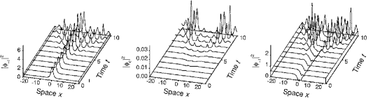
Figure 39: The evolution of the two-component polar soliton on the CW background, given by Eq. (196), under the action of initial random perturbations added to the $\phi_{0}$ and $\phi_{\pm 1}$ components. Parameters are $\nu=+1$, $q=-1/2$, and $\mu=-1$. The results rep4oduced from Ref. 6.1

The FM soliton (179) and three-component polar soliton (LABEL:eq_7.22) also exist in the case of $\nu=-1$ and $a>1$, when $\nu+a$ is positive. In this case too, these two soliton species provide for the energy minimum, simply because the other solitons, (182) , (187) , (LABEL:eq_7.20) , and (LABEL:eq_7.21) do not exist at $\nu=-1$.

For $\nu=+1$ and $-1<a<0$, i.e., attractive spin-independent and repulsive spin-exchange interactions in Eqs. (177), Hamiltonian (195) is smaller than the competing one (180), which means that the two-component polar soliton (187) plays the role of the ground state in this case, as only it, among all the polar solitons whose Hamiltonian is given by expression (195), is dynamically stable in direct simulations (for $-1<a<+1$, see above). As the FM soliton (179) and three-component polar one (LABEL:eq_7.22) also exist and are stable in this region, but correspond to greater energy, they represent metastable states here. Finally, for $\nu$ $=+1$ and $a<-1$, there are no stable solitons.

Dependence $N(\mu)$ for each solution family provides an additional characteristic of the soliton stability. Indeed, the well-known known Vakhitov-Kolokolov criterion 6.4 ; 4.11 states that a necessary stability condition for the soliton family supported by a self-attractive nonlinearity is $dM/d\mu<0$. It guarantees that the soliton cannot be unstable against perturbations with real eigenvalues, but does not say anything about oscillatory perturbations modes appertaining to complex eigenvalues. Obviously, both relations, given by Eqs. (180) and (195), satisfy the criterion, i.e., solitons may be unstable only against perturbations that grow in time with oscillations. Indeed, numerical results which illustrate the evolution of unstable solitons, see Figs. 34-37, clearly suggest that the instability, if any, is oscillatory.

VII.2.6 Finite-background solitons

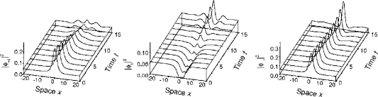
Figure 40: The same as in Fig. 39, but for the finite-background soliton (LABEL:eq_7.25). Parameters are $\nu=a=1$ and $\mu=-0.36$. The results are reproduced from Ref. 6.1 .

In special cases, it is possible to find analytical solutions for solitons sitting on a CW background. Namely, for $\nu=1$ and $a=-1/2$, one can find a two-component polar soliton with a CW background attached to it, in the following form:

$$\phi_{0} = 0,$$

$$\phi_{+1} = \sqrt{-\mu}\left[\frac{1}{\sqrt{2}}\pm\frac{1}{\cosh\left(\sqrt{-\mu}x\right)}\right]\exp\left(-i\mu t\right),$$ (196)

$$\phi_{-1} = \sqrt{-\mu}\left[\frac{1}{\sqrt{2}}\mp\frac{1}{\cosh\left(\sqrt{-\mu}x\right)}\right]\exp\left(-i\mu t\right).$$

For $\nu=a=1$, it is also possible to find a three-component polar solution with the background,

$$\phi_{+1} = \phi_{-1}=\frac{1}{2}\sqrt{-\mu}\left[\frac{1}{\sqrt{2}}\pm\frac{1}{\cosh\left(\sqrt{-\mu}x\right)}\right]\exp\left(-i\mu t\right),$$

$$\phi_{0} = \frac{1}{2}\sqrt{-\mu}\left[\frac{1}{\sqrt{2}}\mp\frac{1}{\cosh\left(\sqrt{-\mu}x\right)}\right]\exp\left(-i\mu t\right).$$

The stability of solutions (196) and (LABEL:eq_7.25) was tested by simultaneously perturbing the $\phi_{0}$ and $\phi_{\pm 1}$ components by small uniformly distributed random perturbations. Figures 39 and 40 show that both solutions are unstable, although the character of the instability is different: in the former case, the soliton’s core seems stable, while the CW background appears to be modulationally unstable. In the latter case, which is shown in Fig. 40, the background is modulationally stable, but the core of the soliton (LABEL:eq_7.25) clearly features oscillatory instability.

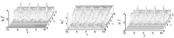
Figure 41: The nonlinear development of the modulation instability, as per exact solution (210), under conditions $k=2\eta$ and $\alpha_{c}^{2}+\beta_{c}^{2}>\xi^{2}$. Parameters are $k=0.6$, $\eta=0.3$, $\xi=1$, $\alpha=\beta=$ $\gamma=\exp\left(-8\right)$, $\alpha_{c}=1.2$, and $\beta_{c}=0$. The results are reproduced from Ref. 6.1 .

MI of the CW background in solution (196) is obvious, as, even without exciting the $\phi_{0}$ field, i.e., in the framework of the reduced equations (177), with $\nu+a=1/2$ and $\nu-a=3/2$, any CW solution is subject to MI. As concerns the excitation of the $\phi_{0}$ field, an elementary consideration shows that the CW part of solution (196) exactly corresponds to the threshold of the parametric instability driven by term $2a\phi_{+1}\phi$ _-1 $\phi_{0}^{\ast}$ in the last equation of system (172). Actually, Fig. 39 demonstrates that the parametric instability sets in, which is explained by a conjecture that the initial development of the above-mentioned MI, that does not involve the $\phi_{0}$ field, drives the perturbed system across the threshold of the parametric instability.

VII.3 The Darboux transform (DT) and nonlinear development of MI

The integrable case, with $\nu=a=1$, which corresponds to the attractive interactions, makes it possible to develop deeper analysis of MI. As mentioned above, the spinor BEC obeys the integrability condition if a special but physically possible constraint (178) is imposed on the scattering lengths of collisions between atoms. Then, Eqs. (172) can be rewritten as a $2\times 2$ matrix NLS equation

$$i\frac{\partial\mathbf{Q}}{\partial t}+\frac{\partial^{2}\mathbf{Q}}{\partial x^{2}}+2\mathbf{QQ}^{{\dagger}}\mathbf{Q=0,}\text{ \ \ }\mathbf{Q\equiv}\left(\begin{array}[]{cc}\phi_{+1}&\phi_{0}\\ \phi_{0}&\phi_{-1}\end{array}\right),$$ (198)

which is a completely integrable system Wadati . DT for Eqs. (198) can be derived from the respective Lax pair, which is 6.5 ; Wadati

$$\frac{\partial\mathbf{\Psi}}{\partial x}=\mathbf{U\Psi,}\frac{\partial\mathbf{\Psi}}{\partial t}=\mathbf{V\Psi.}$$ (199)

Here $\mathbf{U}=\lambda\mathbf{J}+\mathbf{P}$ and $\mathbf{V}=2i\lambda^{2}\mathbf{J}+2i\lambda\mathbf{P}+i\mathbf{W}$, with

$$\mathbf{J} = \left(\begin{array}[]{cc}\mathbf{I}&\mathbf{0}\\ \mathbf{0}&-\mathbf{I}\end{array}\right),\text{ }\mathbf{P}=\left(\begin{array}[]{cc}\mathbf{0}&\mathbf{Q}\\ -\mathbf{Q}^{{\dagger}}&\mathbf{0}\end{array}\right),$$ (200e)

$$\mathbf{W} = \left(\begin{array}[]{cc}\mathbf{QQ}^{{\dagger}}&\frac{\partial}{\partial x}\mathbf{Q}\\ \frac{\partial}{\partial x}\mathbf{Q}^{{\dagger}}&-\mathbf{Q}^{{\dagger}}\mathbf{Q}\end{array}\right),$$ (200h)

where $$\mathbf{I} \mathbf{0} \mathbf{\Psi=}\left(\mathbf{\Psi}_{1},\mathbf{\Psi}_{2}\right)^{\mathrm{T}} \lambda \mathbf{\Psi}_{1} \mathbf{\Psi}_{2} 2\times 2 \lambda \partial\mathbf{U}/\partial r-\partial\mathbf{V}/\partial x+\mathbf{UV}-\mathbf{VU}=0$$ and denote the unit and zero matrices, is the matrix eigenfunction corresponding to , and are matrices, and is the spectral parameter. Accordingly, Eq. (198) is tantamount to the compatibility condition of the overdetermined linear system (199), .

Based on the Lax pair (199), one introduces a transformation in the form of

$$\widetilde{\mathbf{\Psi}}=\left(\lambda-\mathbf{S}\right)\mathbf{\Psi,~{}S}=\mathbf{D\Lambda D}^{-1},~{}\mathbf{\Lambda=}\left(\begin{array}[]{cc}\lambda_{1}\mathbf{I}&\mathbf{0}\\ \mathbf{0}&\lambda_{1}\mathbf{I}\end{array}\right),$$ (201)

where $\mathbf{D}$ is a nonsingular matrix satisfying equation $\partial\mathbf{D/}\partial x=\mathbf{JD\Lambda}+\mathbf{PD}$. Further, letting

$$\frac{\partial\widetilde{\mathbf{\Psi}}}{\partial x}=\widetilde{\mathbf{U\Psi}},\text{ }\widetilde{\mathbf{U}}=\lambda\mathbf{J}+\mathbf{P}_{1}\text{,\ }\mathbf{P}_{1}\equiv\left(\begin{array}[]{cc}\mathbf{0}&\mathbf{Q}_{1}\\ \mathbf{-Q}_{1}^{{\dagger}}&\mathbf{0}\end{array}\right),$$ (202)

one obtains

$$\mathbf{P}_{1}=\mathbf{P}+\mathbf{JS}-\mathbf{SJ}.$$ (203)

One can also verify the following involution property of the linear equations written above: if $\mathbf{\Psi=}\left(\mathbf{\Psi}_{1},\mathbf{\Psi}_{2}\right)^{\mathrm{T}}$ is an eigenfunction corresponding to $\lambda$, where $\mathbf{\Psi}_{j}$ are $2\times 2$ matrices, then $\left(-\mathbf{\Psi}_{2}^{\ast},\mathbf{\Psi}_{1}^{\ast}\right)^{\mathrm{T}}$ is an eigenfunction corresponding to $-\lambda^{\ast}$. Thus one can take $\mathbf{D}$ as

$$\mathbf{D=}\left(\begin{array}[]{cc}\mathbf{\Psi}_{1}&-\mathbf{\Psi}_{2}^{\ast}\\ \mathbf{\Psi}_{2}&\mathbf{\Psi}_{1}^{\ast}\end{array}\right),\text{ }\mathbf{\Lambda=}\left(\begin{array}[]{cc}\lambda\mathbf{I}&\mathbf{0}\\ \mathbf{0}&-\lambda^{\ast}\mathbf{I}\end{array}\right),$$ (204)

to obtain

$$\mathbf{S}=\lambda\left(\begin{array}[]{cc}\mathbf{I}&\mathbf{0}\\ \mathbf{0}&\mathbf{I}\end{array}\right)+\left(\lambda+\lambda^{\ast}\right)\left(\begin{array}[]{cc}-\mathbf{S}_{11}&\mathbf{S}_{12}\\ \mathbf{S}_{21}&-\mathbf{S}_{22}\end{array}\right),$$ (205)

where the matrix elements of $\mathbf{S}$ are given by

$$\mathbf{S}_{11} = \left(\mathbf{I}+\mathbf{\Psi}_{1}\mathbf{\Psi}_{2}^{-1}\mathbf{\Psi}_{1}^{\ast}\mathbf{\Psi}_{2}^{\ast^{-1}}\right)^{-1},\text{ \ }\mathbf{S}_{12}=\left(\mathbf{\Psi}_{2}\mathbf{\Psi}_{1}^{-1}+\mathbf{\Psi}_{1}^{\ast}\mathbf{\Psi}_{2}^{\ast^{-1}}\right)^{-1},$$ (206)

$$\mathbf{S}_{21} = \left(\mathbf{\Psi}_{2}^{\ast}\mathbf{\Psi}_{1}^{\ast^{-1}}+\mathbf{\Psi}_{1}\mathbf{\Psi}_{2}^{-1}\right)^{-1},\text{ }\mathbf{S}_{22}=\left(\mathbf{I}+\mathbf{\Psi}_{2}\mathbf{\Psi}_{1}^{-1}\mathbf{\Psi}_{2}^{\ast}\mathbf{\Psi}_{1}^{\ast^{-1}}\right)^{-1}.$$ (207)

Finally, DT for Eq. (198) follows from Eq. (203), taking the form of

$$\mathbf{Q}_{1}=\mathbf{Q+}2\left(\lambda+\lambda^{\ast}\right)\mathbf{S}_{12}.$$ (208)

From Eqs. (208) and (199) it can be deduced that Eq. (208) generates a new solution $\mathbf{Q}_{1}$ for Eq. (211a), once seed solution $\mathbf{Q}$ is known. In particular, a one-soliton solution can be generated if the seed is a trivial zero state. Next, taking $\mathbf{Q}_{1}$ as the new seed solution, one can derive from Eq. (208) the corresponding two-soliton solution. The procedure can be continued to generate multisoliton solutions.

In what follows, solutions to Eq. (198) are considered under nonzero boundary conditions. The simplest among them is the CW solution with constant densities:

$$\mathbf{Q}_{c}=-\mathbf{A}_{c}\exp\left[i\varphi_{c}\right]\text{, \ \ }\mathbf{A}_{c}\equiv\left(\begin{array}[]{cc}\beta_{c}&\alpha_{c}\\ \alpha_{c}&-\beta_{c}\end{array}\right),\text{ \ }\varphi_{c}\equiv kx+\left[2\left(\alpha_{c}^{2}+\beta_{c}^{2}\right)-k^{2}\right]t,$$ (209)

where $\alpha_{c}$ and $\beta_{c}$ are real constants and $k$ is a wave number. In this solution, the constant densities of components $\phi_{\pm 1}$ are equal, while their signs are opposite.

Applying the above DT to the CW solution $\mathbf{Q}_{c}$, solving Eqs. (199) for this case, and employing Eq. (208), one obtains a new family of solutions of Eq. (198), in the form of

$$\mathbf{Q}_{1}=\left[\mathbf{A}_{c}+4\xi\left(\mathbf{I}+\mathbf{AA}^{\ast}\right)^{-1}\mathbf{A}\right]\exp\left(i\varphi_{c}\right).$$ (210)

Here the following definitions are used:

$$\mathbf{A} = \left[\mathbf{\Pi}\exp\left(\theta-i\varphi\right)+\kappa^{-1}\mathbf{A}_{c}\right]\left[\kappa^{-1}\mathbf{A}_{c}\mathbf{\Pi}\exp\left(\theta-i\varphi\right)+\mathbf{I}\right]^{-1},$$ (211a)

$$\theta = M_{I}x+\left[2\xi M_{R}-\left(k+2\eta\right)M_{I}\right]t,$$ (211b)

$$\varphi = M_{R}x-\left[2\xi M_{I}+\left(k+2\eta\right)M_{R}\right],$$ (211c)

$$M = \sqrt{\left(k+2i\lambda\right)^{2}+4\left(\alpha_{c}^{2}+\beta_{c}^{2}\right)}=M_{R}+iM_{I},$$ (211d)

where $$\kappa\equiv\frac{1}{2}\left(ik-2\lambda+iM\right), \lambda=\xi+i\eta \mathbf{\Pi=}\left(\begin{array}[]{cc}\beta&\alpha\\ \alpha&\gamma\end{array}\right) \xi=0 \phi_{\pm 1}$$ is the spectral parameter, and is an arbitrary complex symmetric matrix. Solution (210) reduces back to CW (209) when . Note that the three-component polar soliton (LABEL:eq_7.25), considered in the previous subsection, is not a special example of solution (210), because the background fields in components in solution (LABEL:eq_7.25) have identical signs.

In particular, with zero background, $\mathbf{A}_{c}=\mathbf{O}$, Eq. (210) yields a soliton solution:

$$\mathbf{Q}_{1}=\frac{4\xi\left[\mathbf{\Pi}_{1}\exp\left(-\theta_{1}\right)+\left(\mathbf{\sigma}^{y}\mathbf{\Pi}_{1}^{\ast}\mathbf{\sigma}^{y}\right)\exp\left(\theta_{s}\right)\det\mathbf{\Pi}_{1}\right]}{\exp\left(-2\theta_{s}\right)+1+\exp\left(2\theta_{s}\right)\left|\det\mathbf{\Pi}_{1}\right|^{2}}\exp\left(i\varphi_{s}\right),$$ (212)

where $\theta_{s}=2\xi\left(x-4\eta t\right)-\theta_{0}$, $\varphi_{s}=2\eta x+4\left(\xi^{2}-\eta^{2}\right)t$, $\theta_{0}$ is an arbitrary real constant which determines the initial position of the soliton, $\mathbf{\sigma}^{y}$ is the Pauli matrix, and $\mathbf{\Pi}_{1}$ is the polarization matrix 6.6 ,

$$\mathbf{\Pi}_{1}=\left(2\left|\alpha\right|^{2}+\left|\beta\right|^{2}+\left|\gamma\right|^{2}\right)^{-1/2}\mathbf{\Pi\equiv}\left(\begin{array}[]{cc}\beta_{1}&\alpha_{1}\\ \alpha_{1}&\gamma_{1}\end{array}\right).$$ (213)

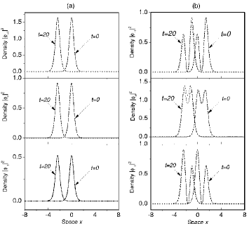
Figure 42: The evolution of the density distribution in the soliton, as obtained from solution (210) by adding a random time-dependent perturbation of the nonlinear-coupling constant $a$, with the perturbation amplitude $\pm 5\%$. Parameters are $\nu=a=1$ (as concerns the unperturbed value of $a$), $\xi=1$, $\eta=-0.03$, and $\theta_{0}=0$. (a) The FM soliton, with $\alpha_{1}=0.48$, $\beta_{1}$ and $\gamma_{1}$ determined by conditions $\alpha_{1}^{2}=\beta_{1}\gamma_{1}$ and $2\left|\alpha_{1}\right|^{2}+\left|\beta_{1}\right|^{2}+\left|\gamma_{1}\right|^{2}=1$; (b) the polar soliton, with $\alpha_{1}=0.53$ and $\beta_{1}=0.43$, $\gamma_{1}$ being determined by condition $2\left|\alpha_{1}\right|^{2}+\left|\beta_{1}\right|^{2}+\left|\gamma_{1}\right|^{2}=1$. Solid and dotted curves show, respectively, the exact solutions and the perturbed ones, produced by numerical simulations. The results are reproduced from Ref. 6.1 .

Solitons (212) are tantamount to ones found in Ref. 6.6 , where they were classified into the above-mentioned types, viz., the FM and polar ones. Indeed, one can see from expression (212) that, when $\det\mathbf{\Pi}_{1}=0$, soliton (212) represents a FM state. However, when $\det\mathbf{\Pi}_{1}\neq 0$, solution (212) may have two peaks, corresponding to a polar state.

Another relevant example of exact solutions (210) describes the onset and nonlinear development of MI of CW states. It can be obtained by noting that, under conditions $k=2\eta$ and $\alpha_{c}^{2}$M $\beta_{c}^{2}$M$\xi^{2}$, Eq. (211d) yields $M_{I}=0$, hence there is no dependence on $x$ in expression (211b), and the solution features no localization. Instead, it is periodic in $x$, through the $x$ dependence of $\varphi$, as given by Eq. (211c); in this connection, note that

$$M_{R}^{2}=4\left(\alpha_{c}^{2}+\beta_{c}^{2}\right)-4\xi^{2}$$ (214)

does not vanish when $M_{I}=0$. This spatially periodic state represents a particular mode of the nonlinear development of MI, in the exact form. To look at it in detail, one can take a special case with $\mathbf{\Pi}=\epsilon\mathbf{E}$, where $\mathbf{E}$ is a matrix with all elements equal to $1$, and $\epsilon$ is a small amplitude of the initial perturbation added to the CW background, with the aim to initiate the onset of MI. Indeed, the linearization of the initial profile of solution (210) with respect to $\epsilon$ yields

$$\mathbf{Q}_{1}(x,0)\approx\left[\mathbf{A}_{c}\rho-\epsilon\chi_{1}\mathbf{E}\cos\left(M_{R}x\right)-\epsilon\chi_{2}\mathbf{\sigma}^{z}\mathbf{\sigma}^{x}\mathbf{A}_{c}\exp\left(iM_{R}x\right)\right]\exp\left(ikx\right),$$ (215)

where $\rho\equiv 1-\xi\left(2\xi+iM_{R}\right)/\left(\alpha_{c}^{2}+\beta_{c}^{2}\right)$ with $\left|\rho\right|=1,$ $\chi_{1}\equiv\xi M_{R}\left(2i\xi-M_{R}\right)/\left(\alpha_{c}^{2}+\beta_{c}^{2}\right)$, $\chi_{2}\equiv\beta_{c}\chi_{1}/\left(\alpha_{c}^{2}+\beta_{c}^{2}\right),$ $M_{R}=2\sqrt{\alpha_{c}^{2}+\beta_{c}^{2}-\xi^{2}}$, and $\mathbf{\sigma}^{x,z}$ are the Pauli matrices. Clearly, the first term in Eq. (215) represents the CW background, while the second and third ones are small spatially modulated perturbations.

Comparing exact solution (210), obtained in this special case, with results of direct numerical simulations of Eqs. (203) with the initial condition (215), one can verify that the numerical solution is very close to the analytical one, both displaying the development of the MI initiated by the small modulational perturbation in expression (215) (not shown here). Figure 41 displays the solution in terms of densities of the three components, as provided by exact result (210). From this picture one concludes that atoms are periodically transferred, in the spinor BEC, from the spin state $m_{F}=0$ into ones $m_{F}=\pm 1$ and vice versa.

As said above, exact solution (210) of Eqs. (172) is only valid under the special condition $a=1$ (i.e., $2g_{0}=-g_{2}$). In the general case ($a\neq 1$), the onset of the MI can be analyzed directly from Eqs. (172) linearized for small perturbations 6.7 . To this end, take the CW solution (209) with $k=0$, which can be fixed by means of the Galilean transformation, and consider its perturbed version

$$\widetilde{\mathbf{Q}}=\left(\mathbf{A}_{c}+\mathbf{B}\right)\exp\left[2i\nu\left(\alpha_{c}^{2}+\beta_{c}^{2}\right)t\right],\text{ \ }\mathbf{B}=\left(\begin{array}[]{cc}b_{+1}(x,t)&b_{0}(x,t)\\ b_{0}(x,t)&b_{-1}(x,t)\end{array}\right),$$ (216)

where $b_{\pm 1}$ and $b_{0}$ are weak perturbations. Substituting this expression in Eqs. (172), linearizing them, and looking for perturbation eigenmodes in the usual form,

$$b_{j}(x,t)=b_{jR}\cos\left(Kx-\omega t\right)+ib_{jI}\sin\left(Kx-\omega t\right),\text{ \ \ }j=+1,-1,0,$$ (217)

where $b_{jR,I}$ are real amplitudes, the BdG equations give rise to two branches of the dispersion relation between wave number $K$ and frequency $\omega$ of the perturbation,

$$\omega^{2} = K^{2}\left(K^{2}-4a\alpha_{c}^{2}-4a\beta_{c}^{2}\right),$$ (218a)

$$\omega^{2} = K^{2}\left(K^{2}-4\nu\alpha_{c}^{2}-4\nu\beta_{c}^{2}\right).$$ (218b)

The MI sets in when $\omega^{2}$ given by either expression ceases to be real and positive. Obviously, this happens if, at least, one condition

$$K^{2}<4a\left(\alpha_{c}^{2}+\beta_{c}^{2}\right),\text{ }K^{2}<4\nu\left(\alpha_{c}^{2}+\beta_{c}^{2}\right)$$ (219)

holds. Note that these conditions agree with the above exact result, which corresponds to $a=\nu=1$. Indeed, in that case one may identify $K\equiv M_{R}$, according to Eq. (215), and then Eq. (214) entails constraint $M_{R}^{2}<4\left(\alpha_{c}^{2}+\beta_{c}^{2}\right)$, which is identical to conditions (219). Note that the MI may occur in the case of the repulsive spin-independent interactions in Eqs. (172), i.e., for $\nu=-1$, provided that the nonlinear-coupling constant $a$, which accounts for the strength of the spin-dependent interaction, is positive.

The stability of the soliton solutions (212) was explored too, of both the polar and FM types, against finite random variations of the coupling constant $a$ in time. The issue is relevant, as the exact solutions are only available for $a=1$; hence, it is necessary to understand if the solitons survive random deviations of $a$ from this value corresponding to the integrability. Physically, this situation may correspond to a case when the scattering length, which determines the nonlinear coefficient $a$ in Eqs. (172), follows random variations of an external magnetic or laser field which affects the scattering length through FR. The evolution of the density profiles in the thus perturbed solitons is displayed in Fig. 42. This figure demonstrates that the solitons of both the FM and polar types are robust against random changes of $a$, once they are dynamically stable as exact solutions to the integrable version of the model. Note also that the FM soliton seems more robust than its polar counterpart.

VII.4 Conclusion of the section

Soliton states have been presented in the model based on the coupled GP equations describing the dynamics of spinor BEC with atomic spin $F=1$. In the general nonintegrable version of the model, several types of elementary exact soliton solutions are reported, which include one, two, or three components, and represent either polar or FM solitons. Their stability is checked by direct simulations and, in some cases, in an exact analytical form, based on BdG equations for small perturbations. The global stability of the solitons is analyzed by comparing the respective values of the energy for a fixed norm. As the main result, stable ground-state solitons of the polar and FM types have been found. Metastable solitons coexisting with the ground-state ones are possible too, in certain parameter regions.

In the special case of the integrable spinor-BEC model Wadati , DT has been introduced and applied to derive a family of exact solutions on top of the CW background. This family includes a solution that explicitly displays full nonlinear evolution of the MI of the CW state, seeded by a small spatially periodic perturbation. Robustness of one-soliton solutions of both the FM and polar types against finite perturbations of the coupling constant (deviations from the integrability) has been verified by means of direct simulations.

VIII Soliton dynamics in one-dimensional spin-orbit-coupled BEC

This section deals with motion of matter-wave solitons in 1D spin-orbit-coupled (SOC) BEC. It is demonstrated that the spin dynamics of solitons in this system is governed by a nonlinear Bloch equation, which affects the orbital motion of solitons, leading to SOC effects in the motion of macroscopic quantum objects. The solitons perform oscillations with a frequency determined by the interplay of SOC, Raman coupling, and intrinsic nonlinearity 7.2 . Analytical predictions are corroborated by numerical simulations of the underlying system of GP equations.

Results collected in this section are based on Ref. 7.2 .

VIII.1 The model

In the presence of SOC, the dynamics of quasi-1D BEC, elongated in the direction of $z$, is modeled by the GP equation for the pseudo-spinor mean-filed wave function,

$$i\frac{\partial}{\partial t}\left(\begin{array}[]{c}\psi_{\uparrow}\\ \psi_{\downarrow}\end{array}\right)=\widehat{h}_{0}\left(\begin{array}[]{c}\psi_{\uparrow}\\ \psi_{\downarrow}\end{array}\right)+\left(\begin{array}[]{cc}g_{\uparrow\uparrow}\left|\psi_{\uparrow}\right|^{2}&g_{\uparrow\downarrow}\left|\psi_{\downarrow}\right|^{2}\\ g_{\downarrow\uparrow}\left|\psi_{\uparrow}\right|^{2}&g_{\downarrow\downarrow}\left|\psi_{\downarrow}\right|^{2}\end{array}\right)\left(\begin{array}[]{c}\psi_{\uparrow}\\ \psi_{\downarrow}\end{array}\right),$$ (220)

where $\psi_{\sigma}$ are pseudospin components, with $\sigma=\uparrow,\downarrow$ labelling the spin states. These can represent, for instance, the hyperfine states $|1,-1\rangle$ and $|1,0\rangle$ of ⁸⁷Rb atoms 7.1 ; SOC-review1 ; SOC-review2 . Here,

$$\widehat{h}_{0}=-\frac{1}{2}\frac{\partial^{2}}{\partial z^{2}}+V(z)+i\lambda\frac{\partial\sigma_{z}}{\partial z}+\Omega\sigma_{x}+\delta\sigma_{z}$$ (221)

is the single-particle Hamiltonian which includes the Raman-induced SOC with frequency $\Omega$ and strength $\lambda$, while $\delta$ is the Zeeman detuning. Further, $V(z)=\gamma^{2}z^{2}/2$ is the 1D HO trapping potential with aspect ratio $\gamma\equiv\omega_{z}/\omega_{\perp}$, where $\omega_{z}$ and $\omega_{\perp}$ are the trapping frequencies along the longitudinal and transverse directions, respectively. The frequencies and lengths are measured here in units $\omega_{\perp}$ and $a_{\perp}=\sqrt{\hslash/\left(m\omega_{\perp}\right)}$, respectively, and the SOC strength is $\lambda=k_{L}a_{\perp}$, with $k_{L}$ being the momentum transfer. Note that, as the scattering lengths characterizing the inter- and intra-species atomic interactions are very close in the experiment, it is reasonable to assume $SU(2)$-symmetric spin interactions, with all strengths $g_{\sigma\sigma^{\prime}}$ taking a single value, $g$. To focus on SOC effects in the dynamics of solitons, the free space is considered first, while effects of the external trap are discussed afterwards. Note that the SOC term $\sim\lambda$ in Eq. (221) breaks the Galilean invariance of the system of GP equations (220) in the free space (although the total momentum remains a dynamical invariant). The latter fact makes mobility of solitons in the SOC system a nontrivial issue, which is a particular motivation for studying them.

For $\lambda=\Omega=0$, the system reduces to the normal binary BEC without SOC. In this case, Eq. (220) with $g_{\sigma\sigma^{\prime}}\equiv g$ is the integrable Manakov’s system 4.14 . In particular, it produces bright-bright solitons $\psi_{\sigma}=\eta\epsilon_{\sigma}\left[\sqrt{-g}\cosh\left(\eta z\right)\right]^{-1}\exp\left(i\eta^{2}t/2\right)$ for the attractive sign of the nonlinearity, $g<0$, where $\eta^{-1}$ is the soliton’s width, and $|\epsilon_{\uparrow}|^{2}+|\epsilon_{\downarrow}|^{2}=-g/(2\eta)$. Such exact soliton solutions may be naturally used as an initial wave function, while SOC is switched on. Note that the effective single-particle Hamiltonian (221) can be rewritten in the frame transformed by the local pseudospin rotation with angle $\vartheta=2\lambda z$ about the $z$ axis. The transformation adds phase factors $\exp\left(\pm i\lambda z\right)$ to the two components of the wave function.

VIII.2 Approximate analytical results (variational approximation)

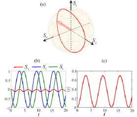
Figure 43: The track of the motion of the spin density on the Bloch sphere (a), and the corresponding evolution of the spin components (b) and center-of-mass coordinate (c) of the soliton for the initially balanced state, with $\theta(t=0)=\pi/4$, and initial phase difference $\varphi_{-}(t=0)=\pi/4$, see Eq. (223). Other parameters are $\Omega=0.5$, $\lambda=0.5\sqrt{\Omega}$, $\delta=0$, and $g=-10$. $z$ and $t$ being measured in units of $a_{\perp}$ and $\omega_{\perp}^{-1}$. The results are reproduced from Ref. 7.2 .

The full GP system (220) is not integrable. Therefore, it is relevant to employ VA for the analysis of the soliton dynamics 3.5 ; 7.2 , making use of the Lagrangian

$$L=\int_{-\infty}^{+\infty}\left\{\frac{i}{2}\sum_{\sigma=\uparrow,\downarrow}\left[\psi_{\sigma}^{\ast}(\psi_{\sigma})_{t}-\psi_{\sigma}(\psi_{\sigma}^{\ast})_{t}\right]-\mathcal{H}\right\}dz,$$ (222)

where $\mathcal{H}$ is the Hamiltonian density of system (220). In the case of the attractive nonlinearity, $g<0$, the following variational ansatz for bright-bright solitons, with the total norm fixed to be $1$, was introduced in Ref. 7.2 :

$$\left(\begin{array}[]{c}\psi_{\uparrow}\\ \psi_{\downarrow}\end{array}\right)=\sqrt{\frac{\eta}{2}}\left(\begin{array}[]{c}\sin\theta\cosh^{-1}\left(\eta z+\xi\right)\exp\left[i\left(k_{\uparrow}z+\varphi_{\uparrow}\right)\right]\\ \cos\theta\cosh^{-1}\left(\eta z+\xi\right)\exp\left[i\left(k_{\downarrow}z+\varphi_{\downarrow}\right)\right]\end{array}\right),$$ (223)

where $\theta$, $\eta$, $\xi$, $k_{\sigma}$, $\varphi_{\sigma}$ are time-dependent variational parameters. Here, $\theta$ determines the population imbalance between the pseudospin components, $\eta^{-1}$ defines their common width, $k_{\sigma}$ is the wave number, and $\varphi_{\sigma}$ the phase.

Inserting ansatz (223) into the Lagrangian and performing the integration, one obtains the effective Lagrangian,

$$L = \frac{\xi}{\eta}\frac{dk_{+}}{dt}-\frac{\xi}{\eta}\cos\left(2\theta\right)\frac{dk_{-}}{dt}-\frac{d\varphi_{+}}{dt}+\cos\left(2\theta\right)\frac{d\varphi_{-}}{dt}$$

$$-\frac{1}{2}\left[k_{+}^{2}-2k_{+}k_{-}\cos\left(2\theta\right)+k_{-}^{2}\right]-\frac{1}{6}\eta^{2}-\frac{1}{6}g\eta$$

$$-\frac{\Omega\pi k_{-}\sin\left(2\theta\right)\cos\left(2\varphi_{-}-2k_{-}\xi/\eta\right)}{\eta\sinh\left(\pi k_{-}/\eta\right)}$$

$$+\delta\cos\left(2\theta\right)-\lambda\left[k_{+}\cos\left(2\theta\right)-k_{-}\right],$$

where $k_{\pm}\equiv(1/2)(k_{\uparrow}\pm k_{\downarrow})$ and $\varphi_{\pm}\equiv(1/2)(\varphi_{\uparrow}\pm\varphi_{\downarrow})$. The evolution of the variational parameters is governed by the corresponding Euler-Lagrangian equations. These equations produce simple results, $\eta\approx-g/2$ and $k_{-}\approx\lambda$, in the case of a weak SOC, $\pi\lambda\ll\eta$. Indeed, in the absence of SOC, relation $\eta=-g/2$ holds for the normalized wave function, indicating that the width of the solitons is determined by the nonlinearity, and $k_{-}$ remains equal to the initial relative momentum $\lambda$ between the components of the soliton. As a result, one arrive at a reduced system of dynamical equations, in which $\eta$ and $k_{-}$ are considered as frozen quantities:

$$\frac{d}{dt}k_{+} = 2\widetilde{\lambda}\sin\left(2\theta\right)\sin\phi,$$ (225a)

$$\frac{d}{dt}\phi = -2\widetilde{\Omega}\cot\left(2\theta\right)\cos\phi+2\lambda k_{+}-2\delta,$$ (225b)

$$\frac{d}{dt}\theta = -\widetilde{\Omega}\sin\phi,$$ (225c)

$$\frac{d}{dt}\left\langle z\right\rangle = k_{+}.$$ (225d)

Here, $$\langle z\rangle=\int_{-\infty}^{+\infty}z(|\psi_{\uparrow}|^{2}+|\psi_{\downarrow}|^{2})dz\equiv-\xi/\eta \widetilde{\Omega}\equiv\pi\lambda/[\eta\sinh\left(\pi\lambda/\eta\right)] \phi\equiv 2\varphi_{-}+2k_{-}\langle z\rangle k_{+} \phi \theta \langle z\rangle$$ is the center-of-mass coordinate, , and is the phase difference between the two components of the soliton. Thus, Eqs. (225a)-(225d) account for the dynamical coupling of the center-of-mass momentum , phase difference , population imbalance , and center-of-mass coordinate .

Next, introduce a normalized complex-valued spinor $\chi=(\chi_{\uparrow},\chi_{\downarrow})$ proportional to the two-component wave function, as $\psi_{\sigma}=\sqrt{\rho(z,t)}\chi_{\sigma}$, where $\rho\equiv|\psi_{\uparrow}|^{2}+|\psi_{\downarrow}|^{2}$ is the total density, hence $\chi$ is subject to normalization $|\chi_{\uparrow}|^{2}+|\chi_{\downarrow}|^{2}=1$. Then, one defines spin density $S=\chi^{T}\sigma\chi$, where $\sigma\equiv\{\sigma_{x},\sigma_{y},\sigma_{z}\}$ is the vector set of the Pauli matrices, and one has

$$\{S_{x},S_{y},S_{z}\}=\{\sin\left(2\theta\right)\cos\left(2\lambda z+2\varphi_{-}\right),-\sin\left(2\theta\right)\sin\left(2\lambda z+2\varphi_{-}\right),-\cos\left(2\theta\right)\}$$ (226)

for the ansatz given by Eq. (223). Focusing the consideration on the center-of-mass motion of the soliton, by setting $z=\langle z\rangle=-\xi/\eta$, the evolution of the atomic spin at the soliton’s center-of-mass is governed by the following equations:

$$\frac{d}{dt}S_{x} = 2(\lambda c_{1}-\delta)S_{y}-2\lambda^{2}S_{z}S_{y},$$ (227a)

$$\frac{d}{dt}S_{y} = -2\widetilde{\Omega}S_{z}-2(\lambda c_{1}-\delta)S_{x}+2\lambda^{2}S_{z}S_{x},$$ (227b)

$$\frac{d}{dt}S_{z} = 2\widetilde{\Omega}S_{y},$$ (227c)

where $$c_{1}\equiv\lambda S_{z,0} S_{\alpha,0} \alpha=x,y,z$$, with () being initial values of the components. These equations of motion for the soliton’s spin can be rewritten as

$$\frac{d}{dt}\mathbf{S}=\mathbf{S}\times\mathbf{B}_{\mathrm{eff}},\text{ \ \ }\mathbf{B}_{\mathrm{eff}}=\{2\widetilde{\Omega},0,2\lambda^{2}S_{z}-2(\lambda c_{1}-\delta)\}.$$ (228)

This is the Bloch equation for the spin precession under the action of the effective magnetic field, $\mathbf{B}_{\mathrm{eff}}$. The macroscopic SOC for the soliton as a quantum body is exhibited by the effect of the evolution of the spin on the soliton’s longitudinal momentum, resulting in coupled nonlinear dynamics of the soliton’s spin and position.

To construct solutions of the nonlinear Bloch equation, one first integrates Eq. (227a), dividing it by Eq. (227c). This yields $S_{x}=c_{2}-(\lambda^{2}/2)\widetilde{\Omega}^{-1}S_{z}^{2}+(c_{1}\lambda-\delta)\widetilde{\Omega}^{-1}S_{z}$, where $c_{2}\equiv S_{x,0}+(\delta-c_{1}\lambda)\widetilde{\Omega}^{-1}S_{z,0}+(\lambda^{2}/2)\widetilde{\Omega}^{-1}S_{z,0}^{2}$ is a constant determined by the initial conditions. Next, the analysis focuses on the case of

$$\delta=c_{1}\lambda,$$ (229)

which implies a particular relation between the strengths of the Zeeman splitting and SOC, making the analysis more explicit. By differentiating Eq. (227c), one arrives at a standard equation for anharmonic oscillations for the single spin component $S_{z}$,

$$\frac{d^{2}S_{z}}{dt^{2}}+\Xi S_{z}+2\lambda^{4}S_{z}^{3}=0,$$ (230)

where $\Xi\equiv 4\widetilde{\Omega}(\widetilde{\Omega}-c_{2}\lambda^{2})$ may be positive or negative. Equation (230) has a usual solution,

$$S_{z}(t)=\frac{\sqrt{1-\Xi\tau^{2}}}{2\lambda^{2}\tau}\mathrm{cn}\left(t/\tau,k\right),\text{ }k^{2}=\frac{1}{2}\left(1-\Xi\tau^{2}\right),$$ (231)

where $\mathrm{cn}$ is the Jacobi’s cosine with modulus $k$, and $\tau$ is an arbitrary parameter taking values $\tau<1/\sqrt{\left|\Xi\right|}$. In the case of $\Xi>0$, the linearized version of Eq. (230), which corresponds to $\tau\rightarrow 1/\sqrt{\left|\Xi\right|}$ in Eq. (231), gives rise to free Rabi oscillations with frequency $\sqrt{\left|\Xi\right|}$. In the general case, the frequency given by solution (231), $\omega_{\mathrm{osc}}=\pi/[2\tau K(k)]$, where $K(k)$ is the complete elliptic integral, exceeds $\sqrt{\left|\Xi\right|}$ due to the nonlinear shift. Note also that the nonlinearity may give rise to oscillations in the case of $\Xi<0$, when the Rabi oscillations are impossible.

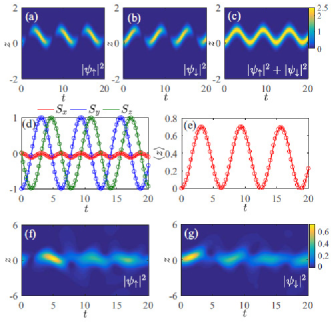
Figure 44: (a-c) The evolution of the density in the two components of the soliton, produced by simulations of Eq. (220) for the initially balanced state with $\theta(t=0)=\pi/4$ and $\varphi_{-}(t=0)=\pi/4$. The parameters are $\Omega=0.5$, $\lambda=0.5\sqrt{\Omega}$, $\delta=0$, and $g=-10$. The spin dynamics and center-of-mass motion of the soliton, generated by these simulations (circles), and by VA based on Eqs. (227a)-(227c) and (232) (solid lines), are depicted in panels (d) and (e). Panels (f) and (g) display decay of the soliton in the case of a weaker atomic interaction, $g=-3$. The results are reproduced from Ref. 7.2 ,

Further, in the spin representation, Eq. (225a) can be written as $dk_{+}/dt=-2\lambda\widetilde{\Omega}S_{y}$, which accounts for the feedback of the evolution of the spin on the center-of-mass momentum (this effect makes the SOC system essentially different from others considered in the present review). This leads to the following equation of motion for the center-of-mass coordinate:

$$\frac{d^{2}\langle z\rangle}{dt^{2}}=-2\lambda\widetilde{\Omega}S_{y}.$$ (232)

In other words, if one considers the soliton as a macroscopic quantum body carrying the intrinsic angular momentum, Eq. (232) represents the driving force, exerted by the intrinsic momentum and acting on the linear momentum. This is, literally, a macroscopic realization of SOC. It is relevant to stress that the mechanism of the soliton’s motion is definitely different from the conventional collective dipole oscillations of BEC in the HO trap. Indeed, in the present case the SOC-induced force which drives the motion of the soliton is the spin precession, rather than the force defined by the external potential.

To illustrate the soliton dynamics in detail, Fig. 44 displays numerical solutions of Eqs. (227a)-(227c) and (232), with initially balanced populations in the two components, which correspond to $\theta(t=0)=\pi/4$ and $\varphi_{-}(t=0)=\pi/4$. First, Fig. 43(a) shows that the soliton’s spin moves along a closed orbit on the Bloch sphere. Accordingly, perfect periodic oscillations of the spin, coupled to the periodic motion of the soliton’s central coordinate, are observed in Figs. 43(b) and (c), respectively. In particular, for weaker SOC, the center-of-mass oscillations can be approximated by $\langle z\rangle\simeq\left(\lambda/\widetilde{\Omega}\right)\sin^{2}\left(\widetilde{\Omega}t\right)$ with amplitude $\lambda/\widetilde{\Omega}$ and period $\pi/\widetilde{\Omega}$, which depend on the strengths of SOC, Raman coupling, and intrinsic BEC nonlinearity.

VIII.3 Numerical results

To test the predictions of VA (i.e., effectively quasi-particle approximation for the motion of the soliton), the system of coupled GP equations (220) was solved numerically in Ref. 7.2 , with the input in the form of the bright-bright soliton,

$$\psi_{\uparrow}=\sqrt{\eta/2}(\sin\theta_{0})\cosh^{-1}\left(\eta z\right)\exp\left[i(\lambda z+\varphi_{\uparrow,0})\right]$$ (233)

$$\psi_{\downarrow}=\sqrt{\eta/2}\left(\cos\theta_{0}\right)\cosh^{-1}\left(\eta z\right)\exp\left[i(-\lambda z+\varphi_{\downarrow,0})\right].$$ (234)

In Figs. 44(a-c), the density of the soliton’s components exhibits robust periodic oscillations, and the soliton maintains its initial hyperbolic-secant profile in the course of many oscillation cycles. Note that, although the initial momenta of the two components are opposite, the soliton does not split. Figures 44(d) and (e) show that results of VA agree very well with the direct GP simulations. For weaker nonlinearity, the simulations show that solitons decay under the action of SOC for $\pi\lambda/\eta>(\pi\lambda/\eta)_{c}\approx 0.4$, as shown in Figs. 44(f) and (g). Furthermore, when condition (229) does not hold, it is found that, besides the SOC-driven oscillations, the soliton exhibits additional linear motion, as can be found, in particular, by simulations for the initially polarized state with $\theta(t=0)=\pi/2$ (not shown here in detail).

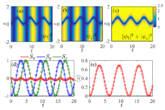
Figure 45: The same as in panels (a)-(e) of Fig. 44, but for the dark soliton, in the case of $g=10$. The results are reproduced from Ref. 7.2 .

Next the case of the repulsive BEC nonlinearity is addressed, which is more relevant to current experiments with SOC condensates 7.1 ; 7.3 . In this case, the following variational ansatz can be used for dark-dark solitons:

$$\left(\begin{array}[]{c}\psi_{\uparrow}\\ \psi_{\downarrow}\end{array}\right)=\sqrt{\frac{\eta}{2}}\left(\begin{array}[]{c}\left(\sin\theta\right)\tanh\left(\eta z+\xi\right)\exp\left(k_{\uparrow}z+\varphi_{\uparrow}\right)\\ \left(\cos\theta\right)\tanh\left(\eta z+\xi\right)\exp\left(k_{\downarrow}z+\varphi_{\downarrow}\right)\end{array}\right),$$ (235)

cf. Eqs. (233) and (234). Inserting ansatz (235) into the Lagrangian, one needs to renormalize the integrals, so as to exclude divergent contributions of the nonvanishing background. The analysis yields the same Euler-Lagrange equations as Eqs. (225b)-(225d), but with $\eta=g/2$ for repulsive $g>0$. The corresponding direct simulations of the GP system were performed in Ref. 7.2 with initial conditions corresponding to the dark-dark soliton,

$$\psi_{\uparrow} = \sqrt{\eta/2}(\sin\theta_{0}\sin)\tanh\left(\eta z\right)\exp\left[i(\lambda z+\varphi_{\uparrow,0})\right],$$ (236)

$$\psi_{\downarrow} = \sqrt{\eta/2}(\cos\theta_{0})\tanh\left(\eta z\right)\exp\left[i(-\lambda z+\varphi_{\downarrow,0})\right].$$ (237)

The results are displayed in Fig. 45, where the dark-dark soliton performs oscillations similar to those displayed above in the case of the bright-bright soliton. Note that the two components of the background alternately disappear and revive, as seen in Figs. 45(a) and (b).

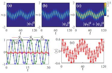
Figure 46: Dynamics of bright-bright solitons in the trapping potential, see Eqs. (238) and (239), with $\gamma=0.1$, the other parameters being the same as in Fig. 44. The results are reproduced from Ref. (7.2 ).

In the experiment, the condensate is trapped in an HO potential, $V(z)=\gamma^{2}z^{2}/2$, which affects the motion of solitons. In this case, the Euler-Lagrange equations for variational parameters $k_{+}$ and $\xi$ are modified to

$$\frac{d}{dt}k_{+}=-2\lambda\widetilde{\Omega}S_{y}+\frac{\gamma^{2}}{\eta}\xi,~{}\frac{d}{dt}\xi=-k_{+}\eta,$$ (238)

with $\eta$ satisfying equation $4\eta^{4}+2g\eta^{3}=\pi^{2}\gamma^{2}$, cf. Eqs. (225a)-(225d). Accordingly, the center-of-mass motion acquires an additional trap-induced term,

$$\frac{d^{2}}{dt^{2}}\langle z\rangle+\gamma^{2}\langle z\rangle=-2\lambda\widetilde{\Omega}S_{y},$$ (239)

which gives rise to additional collective oscillations with period $\simeq 2\pi/\gamma$, as shown in Fig. 46. For a weak trap, the period of the oscillations and the characteristic length scale are much larger than the period and amplitude of the SOC-driven oscillations, therefore the SOC-driven oscillations of the soliton are not conspicuously affected by the trap. Similar results are also produced by the simulations for a dark soliton in the HO trap (oscillations of a trapped single-component dark soliton, in the absence of SOC, were studied in work Busch ).

Finally, it is relevant to briefly discuss conditions for the experimental realization of the predicted dynamical regimes. The Raman-induced SOC has been realized for BEC in the ⁸⁷Rb gas with repulsive atomic interactions. Typically, an elongated condensate of $\sim 10^{4}$ atoms is trapped in a weak HO trap with frequencies $\omega_{\perp}=2\pi\times 85$ $\mathrm{Hz}$ and $\omega_{z}=2\pi\times 5.9$ $\mathrm{Hz}$, and the ratio of the scattering lengths is $a_{\uparrow\uparrow}:a_{\uparrow\downarrow}:a_{\downarrow\downarrow}=1:1$ $:1.005$. In this case, a stationary dark-dark soliton with width $\sim 0.5$ $\mathrm{\mu m}$ can be created at the center of the condensate by means of PIT imprint . Then two $804.1$ nm Raman lasers with intersection angle $20^{\circ}$ are used to induce weak SOC. With the above parameters, the period and amplitude of the SOC-driven oscillations of the dark-dark soliton are about $11$ ms and $2$ $\mathrm{\mu m}$, respectively, which may be further adjusted by varying strengths of the SOC, Raman coupling, and atomic interaction. These estimates clearly suggest that the SOC-driven oscillations can be experimentally observed under available experimental conditions.

VIII.4 Conclusion of the section

In conclusion, it has been shown in this section that the interplay of SOC, Raman coupling, and intrinsic nonlinearity in quasi-1D BEC may realize the mechanism of macroscopic SOC, in the form of a mechanical motion of bright and dark solitons, considered as macroscopic quantum bodies. The soliton’s angular momentum (spin) evolves according to the Bloch equation under the action of an effective magnetic field, and induces a force affecting the motion of the soliton’s central coordinate. The results have been obtained by means of VA and numerical simulations, which demonstrate very good agreement. These findings suggest directions for experimental studies of the motion of matter-wave solitons under the action of SOC.

IX Conclusion of the article

Theoretical and experimental work focused on solitons and other nonlinear modes in BEC and similar physical settings (in particular, nonlinear optics) subject to the temporal, spatial, and spatiotemporal “management”, has grown into a vast research area. In terms of the theory, the central theme is analytical and numerical investigation of the dynamics of solitons and other modes in the framework of the underlying models (chiefly, NLS and GP equations, as well as multicomponent systems of coupled equations), in which coefficients in front of specific linear and nonlinear terms are made functions of time and/or spatial coordinates. Well-known examples are the dispersion management in optics and nonlinearity management in BEC. In this context, basic subjects of the theoretical studies are the existence and stability of solitons and extended nonlinear states in this class of models. In particular, an important direction is search for nontrivial models which may be transformed into well-known integrable equations with constant coefficients, such as the 1D cubic NLS equation and the Manakov’s system. Then, by means of the inverse transformation, one can produce a vast set of exact stable solutions in the original models, using, as inputs, well-known exact solutions of the integrable equations. Search for robust solitons in nonintegrable systems is a still more challenging direction, which has also yielded many nontrivial results. These findings are summarized in the present review. Also included are theoretical results obtained in some other models, which, strictly speaking, do not include spatiotemporal modulation, but the methods and findings elaborated for such models are closely related to those produced in models which explicitly include the spatiotemporal “management”. Particular results, which are collected in the article, are summarized in detail in concluding subsections included in Sections 2-8.

The most essential point which should be stressed to conclude the review is that experimental findings lag far beyond the theoretical predictions. Nevertheless, the remarkable progress in the development of experimental methods in realms of matter waves in BEC, as well as in nonlinear optics, suggest that essential development of the experimental studies in the areas outlined in the present review may be expected. In particular, many theoretical predictions, presented in this review, provide straightforward clues for the experiment.

As concerns further development of the theory, there are many interesting problems to be tackled. In particular, this may be the investigation of 2D and 3D solitons and similar objects, especially solitary vortices and more complex self-trapped modes with an intrinsic topological structure, as well as studies of interactions between two or several solitons, and formation of multi-soliton bound states, in one- and multidimensional settings alike. The study of multidimensional models is most interesting in cases when they cannot be reduced, by means of exact or approximate factorization, to 1D counterparts. As concerns interactions between solitons, they may yield most nontrivial results in models which are not tantamount to integrable equations, hence results of the interactions may be strongly different from familiar elastic collisions.

References

- (1) T. Dauxois and M. Peyrard, Physics of Solitons (Cambridge University Press, Cambridge 2006).
- (2) J. Yang, Nonlinear Waves in Integrable and Nonintegrable Systems (SIAM, Philadelphia, 2010).
- (3) A. Hasegawa and Y. Kodama, Solitons in Optical Communications (Clarendon Press, Oxford, 1995).
- (4) Y. S. Kivshar and G. P. Agrawal, Optical Solitons: From Fibers to Photonic Crystals (Academic Press, San Diego, 2003).
- (5) K. E. Strecker, G. B. Partridge, A. G. Truscott and R. G. Hulet, Bright matter wave solitons in Bose-Einstein condensates, New J. Phys. 5 (2003) 73.
- (6) F. Kh. Abdullaev, A. Gammal, A. M. Kamchatnov, and L. Tomio, Dynamics of bright matter wave solitons in a Bose-Einstein condensate, Int. J. Mod. Phys. B 19 (2005) 3415-3473.
- (7) L. Salasnich, Bright solitons in ultracold atoms, Opt. Quant. Electron. 49 (2017) 409.
- (8) B. A. Malomed, Soliton Management in Periodic Systems, Springer, New York, 2006.
- (9) S. K. Turitsyn, B. G. Bale, and M. P. Fedoruk, Dispersion-managed solitons in fibre systems and lasers, Phys. Rep. 521 (2012) 135-203.
- (10) J. H. B. Nijhof, N. J. Doran, W. Forysiak, and F. M. Knox, Stable soliton-like propagation in dispersion managed systems with net anomalous, zero and normal dispersion, Electron. Lett. 33, 1726-1727 (1997).
- (11) A. N. Niculae, W. Forysiak, A. J. Gloag, J. H. B. Nijhof, and N. J. Doran, Soliton collisions with wavelength-division multiplexed systems with strong dispersion management, Opt. Lett. 23, 1354-1356 (1998).
- (12) D. J. Kaup, B. A. Malomed, and J. Yang, Collision-induced pulse timing jitter in a wavelength-division-multiplexing system with strong dispersion management, J. Opt. Soc. Am. B 16, 1628-1635 (1999).
- (13) C. C. Mak, K. W. Chow and K. Nakkeeran, Soliton pulse propagation in averaged dispersion-managed optical fiber system. J. Phys. Soc. Jpn. 74 (2005) 1449.
- (14) M. Matuszewski, M. Trippenbach, B. A. Malomed, E. Infeld, and M. Skorupski, Two-dimensional dispersion-managed light bullets in Kerr media, Phys. Rev. E 70, 016603 (2004).
- (15) L. Gao, K. H. Wagner, and R. R. McLeod, All-optical Tb/S 3R wavelength conversion using dispersion-managed light bullets, IEEE J. Sel. Topics Quant. Elect. 14, 625-633 (2008).
- (16) M. Desaix, D. Anderson, and M. Lisak, Variational approach to collapse of optical pulses, J. Opt. Soc. Am. B 8 (1991) 2082-2085.
- (17) I. Towers and B. A. Malomed, Stable (2+1)-dimensional solitons in a layered medium with sign-alternating Kerr nonlinearity. J. Opt. Soc. Am. B 19 (2002) 537-543.
- (18) R. Y. Chiao, E. Garmire and C. H. Townes, Self-trapping of optical beams, Phys. Rev. Lett. 13 (1964) 479-482.
- (19) G. Fibich, The Nonlinear Schrödinger Equation: Singular Solutions and Optical Collapse (Springer, Heidelberg, 2015).
- (20) R. J. Valkenburg and A. M. McIvor, Accurate 3D measurement using a structured light system, Image and Vision Computing 16 (1998) 99-110.
- (21) J. Salvi, J. Pages, and L. Batlle, Pattern codification strategies in structured light systems, Pattern Recognition 37 (2004) 827-849.
- (22) S. Zhang, H, Song and S. Peisen, Novel method for structured light system calibration, Optical Engineering 45 (2006) 083601.
- (23) J. Geng, Structured-light 3D surface imaging: a tutorial, Adv. Opt. Phot. 3 (2011) 128-160.
- (24) A. Forbes, A. Dudley, and M. McLaren, Creation and detection of optical modes with spatial light modulators, Adv. Opt. Phot. 8 (2016) 200-227.
- (25) H. Rubinsztein-Dunlop, A. Forbes, M. V. Berry, M. R. Dennis, D. L. Andrews, M. Mansuripur, C. Denz, C. Alpmann, P. Banzer, T. Bauer, E. Karimi, L. Marrucci, M. Padgett, M. Ritsch-Marte, N. M. Litchinitser, N. P. Bigelow, C. Rosales-Guzman, A. Belmonte, J. P. Torres, T. W. Neely, M. Baker, R. Gordon, A. B. Stilgoe, J. Romero, A. G. White, R. Fickler, A. Willner, G. D. Xie, B. McMorran, and A. M. Weiner, Roadmap on structured light, J. Optics 19 (2017) 013001.
- (26) D. L. Andrews, Structured Light and Its Applications: An Introduction to Phase-Structured Beams and Nanoscale Optical Forces, Elsevier Academic Press, San Diego, 2008.
- (27) D. H. Froula, D. Turnbull, A. S. Davies, T. J. Kessler, D. Haberberger, J. P. Palastro, S. W. Bahk, I. A. Begishev, R. Boni, S. Bucht, J. Katz, and J. L. Shaw, Spatiotemporal control of laser intensity, Nature Phot. 12 (2018) 262-265.
- (28) D. Turnbull, S. W. Bahk, I. A. Begishev, R. Boni, J. Bromage, S. Bucht, A. Davies, P. Franke, D. Haberberger, J. Katz, T. J. Kessler,A. L. Milder, J. P. Palastro, J. L. Shaw, and D. H. Froula, Flying focus and its application to plasma-based laser amplifiers, Plasma Phys. Contr. Fusion 61 (2019) 014022.
- (29) T. T. Simpson, D. Ramsey, P. Franke, N. Vafaei-Najafabadi, D. Turnbull, D. H. Froula, and J. P. Palastro, Nonlinear spatiotemporal control of laser intensity, preprint arXiv:2009.11783.
- (30) K. Henderson, C. Ryu, C. MacCormick, and M. G. Boshier, Experimental demonstration of painting arbitrary and dynamic potentials for Bose–Einstein condensates, New J. Phys. 11 (2009) 043030.
- (31) Received 17
- (32) L. P. Pitaevskii and S. Stringari, Bose-Einstein Condensation (Oxford University Press, Oxford, 2003).
- (33) H. Feshbach, A. K. Kerman, and R. H. Lemmer, Intermediate structure and doorway states in nuclear reactions, Annals of Physics 41 (1967) 230-286.
- (34) C. Chin, R. Grimm, P. Julienne, and E. Tiesinga, Feshbach resonances in ultracold gases, Rev. Mod. Phys. 82 (2010) 1225-1286.
- (35) G. Roati, M. Zaccanti, C. D’Errico, J. Catani, M. Modugno, A. Simoni, M. Inguscio, G. Modugno, 39K Bose-Einstein Condensate with Tunable Interactions. Phys. Rev. Lett. 99 (2007) 010403.
- (36) E. R. I. Abraham, W. I. McAlexander, J. M. Gerton, R. G. Hulet, R. Côté, and A. Dalgarno, Singlet s-wave scattering lengths of 6Li and 7Li. Phys. Rev. A 53 (1996) R3713.
- (37) S. E. Pollack, D. Dries, M. Junker, Y. P. Chen, T. A. Corcovilos, and R. G. Hulet, Extreme tunability of interactions in a 7Li Bose-Einstein condensate, Phys. Rev. Lett. 102 (2009) 090402.
- (38) F. Wang, X. Li, D. Xiong, and D. Wang, A double species 23Na and 87Rb Bose-Einstein condensate with tunable miscibility via an inter-species Feshbach resonance, J. Phys. B At. Mol. Opt. Phys. 49 (2016) 015302.
- (39) P. O. Fedichev, Yu. Kagan, G. V. Shlyapnikov, and J. T. M. Walraven, Influence of nearly resonant light on the scattering length in low-temperature atomic gases, Phys. Ref. Lett. 77 (1996) 2913-2916.
- (40) R. Ciuryło, E. Tiesinga, and P. S. Julienne, Optical tuning of the scattering length of cold alkaline-earth-metal atoms. Phys. Rev. A 71 (2005) 030701(R).
- (41) K. Enomoto, K. Kasa, M. Kitagawa, and Y. Takahashi, Optical Feshbach Resonance Using the Intercombination Transition. Phys. Rev. Lett. 101 (2008) 203201
- (42) M. Yan, B. J. DeSalvo, B. Ramachandhran, H. Pu, and T. C. Killian, Controlling condensate collapse and expansion with an optical Feshbach resonance, Phys. Ref. Lett. 110 (2013) 123201.
- (43) D. J. Papoular, G. V. Shlyapnikov, and J. Dalibard, Microwave-induced Fano-Feshbach resonances. Phys. Rev. A 81 (2010) 041603(R).
- (44) B. Marcelis, B. Verhaar, and S. Kokkelmans, Total control over ultracold interactions via electric and magnetic fields, Phys. Rev. Lett. 100 (2008) 153201.
- (45) S. Jochim, M. Bartenstein, A. Altmeyer, G. Hendl, S. Riedl, C. Chin, J. H. Denschlag and R. Grimm, Bose-Einstein condensation of molecules. Science 302 (2003) 2101.
- (46) I. Vidanović, A. Balaž, H. Al-Jibbouri, and A. Pelster, Nonlinear Bose-Einstein-condensate dynamics induced by a harmonic modulation of the s-wave scattering length, Phys. Rev. A 84 (2011) 013618.
- (47) Y. V. Kartashov, B. A. Malomed, and L. Torner, Solitons in nonlinear lattices, Rev. Mod. Phys. 83 (2011) 247-306.
- (48) S.-L. Zhang, Z.-W. Zhou, and B. Wu, Phys. Rev. A 87 (2013) 013633.
- (49) E. Kengne, A. Lakhssassi, and W. M. Liu, Non-autonomous solitons in inhomogeneous nonlinear media with distributed dispersion. Nonlinear Dynamics 97 (2019) 449(R)
- (50) S. L. Cornish, S. T. Thompson, and C. E. Wieman, Formation of bright matter-wave solitons during the collapse of attractive Bose-Einstein condensates, Phys. Rev. Lett. 96 (2006) 170401.
- (51)
- (52) L. W. Clark, A. Gaj, L. Feng and C. Chin, Collective emission of matter-wave jets from driven Bose-Einstein condensates, Nature 551 (2017) 356-359.
- (53) H. Fu, L. Feng, B. M. Anderson, L. W. Clark, J. Hu, J. W. Andrade, C. Chin, and K. Levin, Density waves and jet emission asymmetry in Bose fireworks, Phys. Rev. Lett. 121 (2018) 243001.
- (54) J. H. V. Nguyen, M. C. Tsatsos, D. Luo, A. U. J. Lode, G. D. Telles, V. S. Bagnato, and R. G. Hulet, Parametric excitation of a Bose-Einstein condensate: From Faraday waves to granulation, Phys. Rev. X 9 (2019) 011052.
- (55) F. Kh. Abdullaev, J. G. Caputo, R. A. Kraenkel, and B. A. Malomed, Controlling collapse in Bose-Einstein condensation by temporal modulation of the scattering length, Phys. Rev. A 67 (2003) 013605 (2003).
- (56) H. Saito and M. Ueda, Dynamically stabilized bright solitons in a two-dimensional Bose-Einstein condensate, Phys. Rev. Lett. 90 (2003) 040403.
- (57) G. D. Montesinos, V. M. Pérez-García, and H. Michinel, Stabilized two-dimensional vector solitons, Phys. Rev. Lett. 92 (2004) 133901 (2004).
- (58) A. Itin, T. Morishita, and S. Watanabe, Reexamination of dynamical stabilization of matter-wave solitons, Phys. Rev. A 74 (2006) 033613.
- (59) B. A. Malomed, (INVITED) Vortex solitons: Old results and new perspectives, Physica D 399 (2019) 108-137 (2019).
- (60) M. Matuszewski, E. Infeld, B. A. Malomed, and M. Trippenbach, Fully three dimensional breather solitons can be created using Feshbach resonances, Phys. Rev. Lett. 95 (2005) 050403.
- (61) M.A. Hoefer, J. J. Chang, C. Hamner, P. Engels, Dark-dark solitons and modulational instability in miscible two-component Bose-Einstein condensates. Phys. Rev. A 84 (2011) 041605(R)
- (62) P. G. Kevrekidis and D. J. Frantzeskakis, Solitons in coupled nonlinear Schrödinger models: A survey of recent developments, Reviews in Physics 1 (2016) 140-153.
- (63) C. D’Errico, A. Burchianti, M. Prevedelli, L. Salasnich, F. Ancilotto, M. Modugno, F. Minardi, and C. Fort, Observation of quantum droplets in a heteronuclear bosonic mixture, Phys. Rev. Research 1 (2019) 033155.
- (64) Z. X. Liang, Z. D. Zhang, and W. M. Liu, Dynamics of a bright soliton in Bose-Einstein condensates with time-dependent atomic scattering length in an expulsive parabolic potential, Phys. Rev. Lett. 94 (2005) 050402.
- (65) W.-P. Zhong, R.-H. Xie, M. Belić, N. Petrović, and G. Chen, Exact spatial soliton solutions of the two-dimensional generalized nonlinear Schrödinger equation with distributed coefficients, Phys. Rev. A 78 (2008) 023821.
- (66) Self-trapping of scalar and vector dipole solitary waves in Kerr media W.-P. Zhong, M. R. Belić, G. Assanto, B. A. Malomed, and T. W. Huang, Phys. Rev. A 83 (2011) 043833.
- (67) J. Belmonte-Beitia, V. M. Perez-Garcia, V. Vekslerchik, and V. V. Konotop, Localized nonlinear waves in systems with time- and space-modulated nonlinearities, Phys. Rev. Lett. 100 (2008) 164102.
- (68) S. Rajendrana, P. Muruganandam, and M. Lakshmanan, Bright and dark solitons in a quasi-1D Bose Einstein condensates modelled by 1D Gross Pitaevskii equation with time-dependent parameters, Physica D 239 (2010). 366-386.
- (69) Q.-Y. Li, Z.-D. Li, L. Li, and G.-S. Fu, Nonautonomous bright and dark solitons of Bose-Einstein condensates with Feshbach-managed time-dependent scattering length, Opt. Commun. 283 (2010) 3361-3366.
- (70) B. Li, X.-F. Zhang, Y.-Q. Li, and W. M. Liu, Propagation and interaction of matter-wave solitons in Bose–Einstein condensates with time-dependent scattering length and varying potentials, J. Phys. B At. Mol. Opt. Phys. 44 (2011) 175301.
- (71) W. B. Cardoso, J. Zeng, A. T. Avelar, D. Bazeia, and B. A. Malomed, Bright solitons from the nonpolynomial Schrödinger equation with inhomogeneous defocusing nonlinearities, Phys. Rev. E 88 (2013) 025201.
- (72) R. Radha , P. S. Vinayagam, J. B. Sudharsan, W.-M. Liu, and B. A. Malomed, Engineering bright solitons to enhance the stability of two-component Bose-Einstein condensates, Phys. Lett. A 379, 2977-2983 (2015).
- (73) M. Belić, N. Petrović, W.-P. Zhong, R. H. Xie, and G. Chen, Analytical light bullet solutions to the generalized (3+1)-dimensional nonlinear Schrödinger equation, Phys. Rev. Lett. 101 (2008) 123904.
- (74) N. Petrović, M. Belić, W.-P. Zhong, R. H. Xie, and G. Chen, Exact spatiotemporal wave and soliton solutions to the generalized (3+1)-dimensional Schrödinger equation for both normal and anomalous dispersion, Opt. Lett. 34 (2009) 1609-1611.
- (75) W.-P. Zhong and M. Belić, Three-dimensional optical vortex and necklace solitons in highly nonlocal nonlinear media, Phys. Rev. A 79 (2009) 023804.
- (76) W.-P. Zhong, M. Belić, G. Assanto, and T. Huang, Three-dimensional spatiotemporal vector solitary waves, J. Phys. B: At. Mol. Opt. Phys. 44 (2011) 095403.
- (77) S.-L. Xu, W.-P. Zhong, and M. Belić, Three-dimensional spatiotemporal vector solitary waves in coupled nonlinear Schrödinger equations with variable coefficients, J. Opt. Soc. Am. B 30 (2013) 113-122.
- (78) S. V. Manakov, On the theory of two-dimensional stationary self-focusing of electromagnetic waves. Zh. Eksp. Teor. Fiz. 65 (1973) 505, Sov. Phys. JETP 38 (1974) 248.
- (79) S. K. Suslov, On integrability of nonautonomous nonlinear Schrödinger equations, Proc. Am. Math. Soc. 140 (2012) 3067–3082.
- (80) A. Debnath and A. Khan, On solving cubic-quartic nonlinear Schrödinger equation in a cnoidal trap, Eur. Phys. J. D 74 (2020) 184.
- (81) B. A. Malomed and Yu. A. Stepanyants, The inverse problem for the Gross-Pitaevskii equation, Chaos 20 (2010) 013130.
- (82) L. Salasnich, A. Parola, and L. Reatto, Effective wave equations for the dynamics of cigar-shaped and disk-shaped Bose condensates, Phys. Rev. A 65 (2002) 043614.
- (83) A. Muñoz Mateo and V. Delgado, Effective mean-field equations for cigar-shaped and disk-shaped Bose-Einstein condensates, Phys. Rev. A 77 (2008) 013617.
- (84) V. Dunjko, V. Lorent, and M. Olshanii, Bosons in cigar-shaped traps: Thomas-Fermi Tonks-Girardean regime, and in between, Phys. Rev. Lett. 86 (2001) 5413-5416.
- (85) B. Paredes, A. Widera, V. Murg, O. Mandel, S. Folling, I. Cirac, G. V. Shlyapnikov, T. W. Hansch, and I. Bloch, Tonks-Girardeau gas of ultracold atoms in an optical lattice, Nature 429 (2004) 277-281.
- (86) R. Yamazaki, S Taie, S. Sugawa, and Y. Takahashi, Submicron spatial modulation of an interatomic interaction in a Bose-Einstein condensate, Phys. Rev. Lett. 105 (2010) 050405.
- (87) P. G. Kevrekidis, G. Theocharis, D. J. Frantzeskakis, B. A. Malomed, Feshbach Resonance management for Bose-Einstein condensates, Phys. Rev. Lett. 90 (2003) 230401.
- (88) G. Theocharis, Z. Rapti, P. G. Kevrekidis, D. J. Frantzeskakis, V. V. Konotop, Modulational instability of Gross-Pitaevskii-type equations in 1+1 dimensions, Phys. Rev. A 67, (2003) 063610.
- (89) J. H. V. Nguyen, D. Luo, and R. G. Hulet, Formation of matter-wave soliton trains by modulational instability, Science 356 (2017) 422-426.
- (90) P. J. Everitt, M. A. Sooriyabandara, M. Guasoni, P. B. Wigley, C. H. Wei, G. D. McDonald, K. S. Hardman, P. Manju, J. D. Close, C. C. N. Kuhn, S. S. Szigeti, Y. S. Kivshar, and N. P. Robins, Observation of a modulational instability in Bose-Einstein condensates, Phys. Rev. A 96 (2017) 041601(R).
- (91) S. Raghavan and G. P. Agrawal, Spatiotemporal solitons in inhomogeneous nonlinear media, Opt. Commun. 180, (2000) 377-382.
- (92) F. Chen M. Stepić, C. E. Rüter, D. Runde, D. Kip, V. Shandarov, O. Manela, and M. Segev, Discrete diffraction and spatial gap solitons in photovoltaic LiNbO3 waveguide arrays, Opt. Express 13, (2005) 4314.
- (93) Q. Tian, L. Wu, J.-F. Zhang, B. A. Malomed, D. Mihalache, W. M. Liu, Exact soliton solutions and their stability control in the nonlinear Schrödinger equation with spatiotemporally modulated nonlinearity, Phys. Rev. E 83 (2011) 016602.
- (94) J. Belmonte-Beitia, V. M. Pérez-Garcia, V. Vekslerchik, and P. J. Torres, Lie symmetries and solitons in nonlinear systems with spatially inhomogeneous nonlinearities, Phys. Rev. Lett. 98 (2007) 064102.
- (95) E. T. Whittaker, G. N. Watson, A Course in Modern Analysis, 4th ed., Cambridge University Press, Cambridge, UK, 1990.
- (96) Yu. S. Kivshar, T. J. Alexander, and S. K. Turitsyn, Nonlinear modes of a macroscopic quantum oscillator, Phys. Lett. A 278, (2001) 225–230.
- (97) Y. Zhang and B. Wu, Composition relation between gap solitons and Bloch waves in nonlinear periodic systems, Phys. Rev. Lett. 102, (2009) 093905.
- (98) R. Driben, B. A. Malomed, A. V. Yulin, and D. V. Skryabin, Newton’s cradles in optics: From N-soliton fission to soliton chains, Phys. Rev. A 87 (2013) 063808.
- (99) D. Novoa, B. A. Malomed, H. Michinel, and V. M. Perez-Garcia, Supersolitons: Solitonic excitations in atomic soliton chains, Phys. Rev. Lett. 101 (2008) 144101.
- (100) S. Burger, K. Bongs, S. Dettmer, W. Ertmer, K. Sengstock, A. Sanpera, G. V. Shlyapnikov, and M. Lewenstein, Dark solitons in Bose-Einstein condensates, Phys. Rev. Lett. 83 (1999) 5198-5201.
- (101) S. Stellmer, C. Becker, P. Soltan-Panahi, E. M. Richter, S. Dorscher, M. Baumert, J. Kronjager, K. Bongs, K. Sengstock, Collisions of dark solitons in elongated Bose-Einstein condensates, Phys. Rev. Lett. 101, (2008) 120406.
- (102) N. Meyer, H. Proud, M. Perea-Ortiz, C. O’Neale, M. Baumert, M. Holynski, J. Kronjager, G. Barontini, and K. Bongs, Observation of two-dimensional localized Jones-Roberts solitons in Bose-Einstein condensates, Phys. Rev. Lett. 119 (2017) 150403.
- (103) V. N. Serkin, A. Hasegawa, T. L. Belyaeva, Nonautonomous solitons in external potentials, Phys. Rev. Lett. 98 (2007) 074102.
- (104) L. Wu, J. F. Zhang, and L. Li, Modulational instability and bright solitary wave solution for Bose–Einstein condensates with time-dependent scattering length and harmonic potential, New J. Phys. 9 (2007) 1-13.
- (105) K. D. Moll, A. L. Gaeta, and G. Fibich, Self-similar optical wave collapse: Observation of the Townes profile, Phys. Rev. Lett. 90 (2003) 203902.
- (106) K. Mio, T. Ogino, K. Minami, S. Takeda, A Perturbation method and its application to obliquely propagating nonlinear Alfvén wave, J. Phys. Soc. Jpn. 41, (1976) 2114-2120.
- (107) V. R. Kumar, R. Radha, and M. Wadati, Phase engineering and solitons of Bose–Einstein condensates with two- and three-body interactions. J. Phys. Soc. Jpn., 79 (2010) 074005.
- (108) E. Kengne, A. Lakhssassi, W. M. Liu, and R. Vaillancourt, Phase engineering, modulational instability, and solitons of Gross-Pitaevskii-type equations in 1+1 dimensions, Phys. Rev. E 87, 022914 (2013).
- (109) W. Schopff and W. Zimmermann, Convection in binary fluids: Amplitude equations, codimension-2 bifurcation, and thermal fluctuations. Phys. Rev. E 47 (1993) 1739.
- (110) E. Kengne and W. M. Liu, Exact solutions of the derivative nonlinear Schrödinger equation for a nonlinear transmission line. Phys. Rev. E 73, 026603 (2006).
- (111) M.S. Ruderman, Propagation of solitons of the Derivative Nonlinear Schrödinger equation in a plasma with fluctuating density, Phys. Plasmas 9, (2002) 2940.
- (112) A. M. Kamchatnov, New approach to periodic solutions of integrable equations and nonlinear theory of modulational instability, 286 (1997) 199-270.
- (113) N. Tzoar, M. Jain, Self-phase modulation in long-geometry optical waveguides, Phys. Rev. A 23 (1981) 1266.
- (114) D. Anderson and M. Lisak, Nonlinear asymmetric self-phase modulation and self-steepening of pulses in long optical waveguides, Phys. Rev. A 27 (1983) 1393.
- (115) G. Yang and Y. R. Shen, Spectral broadening of ultrashort pulses in a nonlinear medium, Opt. Lett. 9 (1984) 510-512.
- (116) G. P. Agrawal, Nonlinear Fiber Optics (Academic Press, San Diego, 1995).
- (117) D. J. Kaup and A. C. Newell, Exact solution for a derivative non-linear Schrödinger equation, J. Math. Phys. 19, 798-801 (1978).
- (118) T. B. Benjamin and J. E. Feir, The disintegration of wave trains on deep water, J. Fluid Mech. 27 (1967) 417-430.
- (119) V. Talanov, Focusing of light in cubic media, J. Exp. Theor. Phys. Lett. 11 (1970) 199-201.
- (120) G. Fibich and G. Papanicolaou, Self-focusing in the perturbed and unperturbed nonlinear Schrödinger equation in critical dimension, SIAM J. Appl. Math. 60 (1999) 183-240.
- (121) R. Radhakrishnan, A. Kundu, M. Lakshmanan, Coupled nonlinear Schrödinger equations with cubic-quintic nonlinearity: Integrability and soliton interaction in non-Kerr media, Phys. Rev. E 60, (1999) 3314.
- (122) S.-J. Wang, C.-L. Jia, D. Zhao, H.-G. Luo, J.-H. An, Dark and bright solitons in a quasi-one-dimensional Bose-Einstein condensate, Phys. Rev. A 68, (2003) 015601.
- (123) S. L. Cornish, T. T. Sarah, C. E. Wieman, Formation of Bright Matter-Wave Solitons during the Collapse of Attractive Bose-Einstein Condensates, Phys. Rev. Lett. 96, (2006) 170401.
- (124) P. G. Kevrekidis, G. Theocharis, D. J. Frantzeskakis, B. A. Malomed, Feshbach Resonance Management for Bose-Einstein Condensates, Phys. Rev. Lett. 90 (2003) 230401.
- (125) A. V. Carpentier, H. Michinel, M .I. Rodas-Verde, V. M. Pérez-García, Analysis of an atom laser based on the spatial control of the scattering length, Phys. Rev. A 74 (2006) 013619.
- (126) F. Kh. Abdullaev, Yu. V. Bludov, S. V. Dmitriev, P. G. Kevrekidis, V. V. Konotop, Generalized neighbor-interaction models induced by nonlinear lattices. Phys. Rev. E 77 (2008) 016604.
- (127) H. Sakaguchi and B. A. Malomed, Solitons in combined linear and nonlinear lattice potentials, Phys. Rev. A 81 (2010) 013624.
- (128) W. M. Liu and E. Kengne, Schrödinger equations in nonlinear systems, Springer Nature Singapore Pte Ltd., DOI: https://doi.org/10.1007/978-981-13-6581-2 (2019).
- (129) D. Anderson and M. Lisak, Nonlinear asymmetric self-phase modulation and self-steepening of pulses in long optical waveguides. Phys. Rev. A 27, 1393 (1983).
- (130) I. S. Gradshteyn and I. M. Ryzhik, Table of Integrals, Series, and Products, Seventh Edition, Academic Press, San Diego, 2007.
- (131) E. T. Whittaker and G. N. Watson, A Course of Modern Analysis, Cambridge University Press, Cambridge, 1927.
- (132) F. K. Abdullaev, B. B. Baizakov, and M. Salerno, Stable two-dimensional dispersion-managed soliton, Phys. Rev. E 68 (2003) 066605.
- (133) S. K. Adhikari, Stabilization of bright solitons and vortex solitons in a trapless three-dimensional Bose-Einstein condensate by temporal modulation of the scattering length, Phys. Rev. A 69 (2004) 063613.
- (134) H. W. Schürmann and S. V. Serov, Traveling wave solutions of a generalized modified Kadomtsev-Petviashvili equation. J. Math. Phys. 45 (2004) 2181.
- (135) H. W. Schürmann, Traveling-wave solutions of the cubic-quintic nonlinear Schrödinger equation. Phys. Rev. E 54, (1996) 4312.
- (136) R. A. Battye, N. R. Cooper, and P. M. Sutcliffe, Stable Skyrmions in Two-Component Bose-Einstein Condensates. Phys. Rev. Lett. 88, (2002) 080401.
- (137) D. Anderson, Variational approach to nonlinear pulse propagation in optical fibers, Phys. Rev. A 27 (1983) 3135-3144.
- (138) B. A. Malomed, Variational methods in nonlinear fiber optics and related fields. Prog. Opt. 43 (2002) 71-193.
- (139) V. M. Pérez-García, H. Michinel, J. I. Cirac, M. Lewenstein, and P. Zoller, Dynamics of Bose-Einstein condensates: Variational solutions of the Gross-Pitaevskii equations. Phys. Rev. A 56, (1997) 1424.
- (140) Yu. Kivshar and S. Turitsyn, Spatiotemporal pulse collapse on periodic potentials. Phys. Rev. E 49 (1994) 2536.
- (141) T. S. Yang and W. L. Kath, Analysis of enhanced-power solitons in dispersion-managed optical fibers. Opt. Lett. 22 (1997) 985.
- (142) G. Fibich and G. C. Papanicolaou, A modulation method for self-focusing in the perturbed critical nonlinear Schrödinger equation. Phys. Lett. A 239 (1998) 167.
- (143) F. Kh. Abdullaev and J. G. Caputo, Validation of the variational approach for chirped pulses in fibers with periodic dispersion. Phys. Rev. E 58 (1998) 6637.
- (144) L. Bergé, V. K. Mezentsev, J. J. Rasmussen, P. L. Christiansen, and Yu. B. Gaididei, Self-guiding light in layered nonlinear media. Opt. Lett. 25 (2000) 1037.
- (145) L. Bergé, Wave collapse in physics: principles and applications to light and plasma waves. Phys. Rep. 303, (1998) 259.
- (146) S. L. Cornish, N. R. Claussen, J. L. Roberts, E. A. Cornell, and C. E. Wieman, Stable 85Rb Bose-Einstein Condensates with Widely Tunable Interactions. Phys. Rev. Lett. 85 (2000) 1795.
- (147) L. Li, B. A. Malomed, D. Mihalache, and W. M. Liu, Exact soliton-on-plane-wave solutions for two-component Bose-Einstein condensates, Phys. Rev. E 73 (2006) 066610
- (148) V. G. Makhankov, N. V. Makhaldiani, and O. K. Pashaev, On the integrability and isotopic structure of the one-dimensional Hubbard model in the long wave approximation. Phys. Lett. A 81 (1981) 161
- (149) V. M. Pérez-García and J. B. Beitia, Symbiotic solitons in heteronuclear multicomponent Bose-Einstein condensates. Phys. Rev. A 72 (2005) 033620.
- (150) S. K. Adhikari, Bright solitons in coupled defocusing NLS equation supported by coupling: Application to Bose–Einstein condensation, Physics Letters A 346 (2005) 179-185.
- (151) T.-L. Ho, Spinor Bose condensates in optical traps, Phys. Rev. Lett. 81 (1998) 742-745.
- (152) Y. Kawaguchi and M. Ueda, Spinor Bose-Einstein condensates, Phys. Rep. 520 (2012) 253-381.
- (153) D. M. Stamper-Kurn and M. Ueda, Spinor Bose gases: Symmetries, magnetism, and quantum dynamics, Rev. Mod. Phys. 85 (2013) 1191.
- (154) G. P. Agrawal, Modulation instability induced by cross-phase modulation, Phys. Rev. Lett. 59 (1987) 880-883.
- (155) J. Ieda, T. Miyakawa, and M. Wadati, Exact analysis of soliton dynamics in spinor Bose-Einstein condensates, Phys. Rev. Lett. 93 (2004) 194102.
- (156) L. Li, Zaidong Li, B. A. Malomed, D. Mihalache, and W. M. Liu, Exact soliton solutions and nonlinear modulation instability in spinor Bose-Einstein condensates, Phys. Rev. A 72, (2005) 033611
- (157) H. Pu, C. K. Law, S. Raghavan, J. H. Eberly, and N. P. Bigelow, Spin-mixing dynamics of a spinor Bose-Einstein condensate. Phys. Rev. A 60 (1999) 1463
- (158) N. G. Vakhitov and A. A. Kolokolov, Stationary solutions of the wave equation in a medium with nonlinearity saturation, Radiophys. Quantum Electron. 16 (1973) 783.
- (159) T. Tsuchida and M. Wadati, The Coupled Modified Korteweg-de Vries Equations. J. Phys. Soc. Jpn. 67 (1998) 1175
- (160) J. Ieda, T. Miyakawa, and M. Wadati, Exact Analysis of Soliton Dynamics in Spinor Bose-Einstein Condensates. Phys. Rev. Lett. 93, (2004) 194102
- (161) N. P. Robins, W. Zhang, E. A. Ostrovskaya, and Y. S. Kivshar, Modulational instability of spinor condensates. Phys. Rev. A 64 (2001) 021601(R).
- (162) L. Wen, Q. Sun, Y. Chen, D.-S. Wang, J. Hu, H. Chen, W. M. Liu, G. Juzeliūnas, B. A. Malomed, and A.-C. Ji, Motion of solitons in one-dimensional spin-orbit-coupled Bose-Einstein condensates. Phys. Rev. A 94 (2016) 061602(R).
- (163) Y.-J. Lin, K. Jiménez-García, and I. B. Spielman, Spin-orbit-coupled Bose-Einstein condensates. Nature (London) 471 (2011) 83.
- (164) V. Galitski and I. B. Spielman, Spin-orbit coupling in quantum gases, Nature 494 (2013) 49-54.
- (165) H. Zhai, Degenerate quantum gases with spin-orbit coupling: a review, Rep. Progr. Phys. 78 (2015) 026001.
- (166) L. W. Cheuk, A. T. Sommer, Z. Hadzibabic, T. Yefsah, W. S. Bakr, and M. W. Zwierlein, Spin-injection spectroscopy of a spin-orbit coupled Fermi gas, Phys. Rev. Lett. 109 (2012) 095302.
- (167) T. Busch and J. R. Anglin, Motion of dark solitons in trapped Bose-Einstein condensates, Phys. Rev. Lett. 84 (2000) 2298-2301.