Learning Representations from Audio-Visual
Spatial Alignment

Abstract

We introduce a novel self-supervised pretext task for learning representations from audio-visual content. Prior work on audio-visual representation learning leverages correspondences at the video level. Approaches based on audio-visual correspondence (AVC) predict whether audio and video clips originate from the same or different video instances. Audio-visual temporal synchronization (AVTS) further discriminates negative pairs originated from the same video instance but at different moments in time. While these approaches learn high-quality representations for downstream tasks such as action recognition, their training objectives disregard spatial cues naturally occurring in audio and visual signals. To learn from these spatial cues, we tasked a network to perform contrastive audio-visual spatial alignment of 360°video and spatial audio. The ability to perform spatial alignment is enhanced by reasoning over the full spatial content of the 360°video using a transformer architecture to combine representations from multiple viewpoints. The advantages of the proposed pretext task are demonstrated on a variety of audio and visual downstream tasks, including audio-visual correspondence, spatial alignment, action recognition and video semantic segmentation.

1 Introduction

Human perception is inherently multi-sensory. Since real-world events can manifest through multiple modalities, the ability to integrate information from various sensory inputs can significantly benefit perception. In particular, neural processes for audio and visual perception are known to influence each other significantly. These interactions are responsible for several well known audio-visual illusions such as the “McGurk effect” [39], the “sound induced flash effect” [53] or the “fusion effect” [2], and can even be observed in brain activation studies, where areas of the brain dedicated to visual processing have been shown to be activated by sounds that are predictive of visual events, even in the absence of visual input [14, 59].

In computer vision, the natural co-occurrence of audio and video has been extensively studied. Prior work has shown that this co-occurrence can be leveraged to learn representations in a self-supervised manner, i.e., without human annotations. A common approach is to learn to match audio and video clips of the same video instance [3, 4, 42]. Intuitively, if visual events are associated with a salient sound signature, then the audio can be treated as a label to describe the visual content [50]. Prior work has also demonstrated the value of temporal synchronization between audio and video clips for learning representations for downstream tasks such as action recognition [31, 47].

Since these methods do not need to localize sound sources, they struggle to discriminate visual concepts that often co-occur. For example, the sound of a car can be quite distinctive, and thus it is a good target description for the “car” visual concept. However, current approaches use this audio as a descriptor for the whole video clip, as opposed to the region containing the car. Since cars and roads often co-occur, there is an inherent ambiguity about which of the two produce the sound. This makes it is hard to learn good representations for visual concepts like “cars”, distinguishable from co-occurring objects like “roads” by pure audio-visual correspondence or temporal synchronization. This problem was clearly demonstrated in [52] that shows the poor audio localization achieved with AVC pretext training.

To address this issue, we learn representations by training deep neural networks with 1) 360°video data that contain audio-visual signals with strong spatial cues and 2) a pretext task to conduct audio-visual spatial alignment (AVSA, fig. 1). Unlike regular videos with mono audio recordings, 360°video data and spatial audio formats like ambisonics fully capture the spatial layout of audio and visual content within a scene. To learn from this spatial information, we collected a large 360°video dataset, five times larger than currently available datasets. We also designed a pretext task where audio and video clips are sampled from different viewpoints within a 360°video, and spatially misaligned audio/video clips are treated as negatives examples for contrastive learning. To enhance the learned representations, two modifications to the standard contrastive learning setup are proposed. First, the ability to perform spatial alignment is boosted using a curriculum learning strategy that initially focus on learning audio-visual correspondences at the video level. Second, we propose to reason over the full spatial content of the 360°video by combining representations from multiple viewpoints using a transformer network. We show the benefits of the AVSA pretext task on a variety of audio and visual downstream tasks, including audio-visual correspondence and spatial alignment, action recognition and video semantic segmentation.

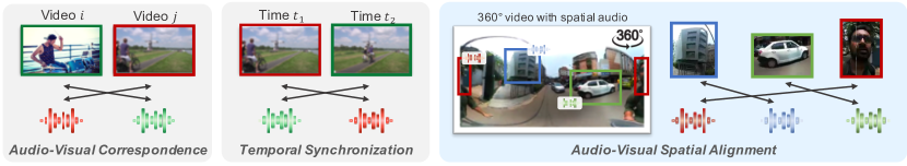
Figure 1: Audio-visual spatial alignment. Prior work on audio-visual representation learning leverages correspondences at the video level. Audio-visual correspondence (AVC) [3, 4, 42] predicts whether a pair of audio and video clips originate from the same video (positive) or different videos (negative). Audio-visual temporal synchronization (AVTS) [47, 31] discriminates negative pairs that are sampled from the same video but different moments in time. However, prior work ignores the spatial cues of audio-visual signals. Instead, we learn representations by performing audio-visual spatial alignment (AVSA) of 360°video and spatial audio. This is accomplished by training a model to distinguish audio and video clips extracted from different viewpoints.

2 Related work

360°media

The increasing availability of 360°data has sparked interest in developing vision systems for 360°imagery. For example, the SUN-360 dataset of static 360°images was collected to learn to recognize viewpoints within a scene [64]. Self-supervised monocular depth and camera motion estimation have also been studied by pairing 360°imagery with depth data [61, 34]. Another common topic of interest is to enhance 360°video consumption by guiding the viewer towards salient viewing angles within a video [66, 10], automating the field-of-view control for 360°video playback [25, 55], or by upgrading mono recordings into spatial sounds [41].

Self-supervised learning

Self-supervised learning methods learn representations without requiring explicit human annotation. Instead of predicting human labels, self-supervision learns representations that are predictive of the input data itself (or parts of it) while imposing additional constraints such as sparsity [35, 45, 44] or invariance [20, 49, 26, 40, 8]. An emergent technique, known as contrastive learning, relies on contrastive losses [20] to learn view invariant representations, where the different views of the data can be generated by data augmentation [63, 40, 23, 9, 24], chunking the input over time or space [46, 21] or using co-occurring modalities [3, 27, 42, 65, 56]. In this work, we also rely on contrastive losses, but utilize contrastive learning to perform audio-visual spatial alignment.

Similarly to the proposed AVSA task, spatial context has previously been used in visual representation learning. For example, [43, 12, 28] try to predict the relative locations of image or video patches, and [21] uses contrastive learning to learn representations that are predictive of their spatio-temporal location. However, as shown in [42], using visual content as both the input and target for representation learning can yield sub-optimal representations, as low-level statistics can be explored to perform the task without learning semantic features. Our approach addresses this issue by leveraging the spatial context provided by a co-occurring modality (audio) that also contains strong spatial cues.

Audio-visual learning

The natural co-occurrence of vision and sound has been successfully used in various contexts such as visually guided source separation and localization [16, 18, 68, 67, 15], and audio spatialization [41, 17]. Audio-visual correspondences [3, 4] have also been used for learning representations for objects and scenes in static images [3, 4, 48], action recognition in video [47, 31, 42, 1], to perform temporal synchronization [11, 22, 47, 31] and audio classification [5]. As discussed in fig. 1, prior work is often implemented either by predicting audio-visual correspondences at the video level [3, 4, 42] or performing temporal synchronization using out-of-sync clips as hard negatives [47, 31]. However, [52] shows that basic audio-visual correspondences are ill-equipped to identify and localize sound sources in the video. We argue that this is because audio-visual correspondences are imposed by matching audio to the entire video clip. Thus, there is little incentive to learn discriminative features for objects that often co-occur. To address this issue, we explore the rich spatial cues present in both the 360°video and spatial audio. By learning to spatially align visual and audio contents, the network is encouraged to reason about the scene composition (i.e. the locations of the various sources of sound), thus yielding better representations for downstream tasks.

3 Audio-visual spatial alignment

We learn audio-visual representations by leveraging spatial cues in 360°media. 360°video and spatial audio encode visual and audio signals arriving from all directions $(\theta,\phi)$ around the recording location, where $\theta$ denotes the longitude (or horizontal) angle, $\phi$ the latitude (or elevation) angle. We adopt the equi-rectangular projection as the 360°video format and first-order ambisonics [19] for the spatial audio. Both formats can be easily rotated and/or decoded into viewpoint specific clips.

3.1 Pretext task

Regressive AVSA

A straight-forward implementation of audio-visual spatial alignment is to generate random rotations $R$ of either the video or audio so as to create an artificial misalignment between them. A model can then be trained to predict the applied transformation by solving

$$\min_{f_{v},f_{a},g}\mathbb{E}_{v,a,R}\left\{d\left[g(f_{v}(v),f_{a}(R(a))),R\right]\right\},$$ (1)

where $f_{v}$ and $f_{a}$ are the video and audio encoders, $g$ a rotation regression head, and $d$ the distance between the predicted and ground-truth rotations $R$. However, this implementation has several disadvantages. Due to the continuous nature of the target variable $R$, the loss of (1) is difficult to optimize. Also, the task is defined on the full 360°video $v$, which limits the use of data augmentation techniques such as aggressive cropping that are critical for self-supervised learning.

Contrastive AVSA

Inspired by recent advances in contrastive learning [20, 46, 63, 56, 42], we propose to solve the audio-visual spatial alignment task in a contrastive fashion. As shown in fig. 1, given a 360°audio-video sample $(v_{i},a_{i})$, $K$ video and audio clips $\{(v_{i}^{k},a_{i}^{k})\}_{k=1}^{K}$ are extracted from $K$ randomly sampled viewing directions $\{(\theta_{k},\phi_{k})\}_{k=1}^{K}$. Video clips $v_{i}^{k}$ are obtained by extracting normal field-of-view (NFOV) crops using a Gnomonic projection [62] centered around $(\theta_{k},\phi_{k})$, and audio clips $a_{i}^{k}$ by realigning the global frame of reference of the ambisonics signal such that the frontal direction points towards $(\theta_{k},\phi_{k})$ [32]. Audio-visual spatial alignment is then encouraged by tasking a network to predict the correct correspondence between the $K$ video $\{v_{i}^{k}\}_{k=1}^{K}$ and the $K$ audio $\{a_{i}^{k}\}_{k=1}^{K}$ signals.

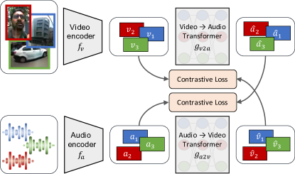
figure[.55][][t] figure[.38][][t]

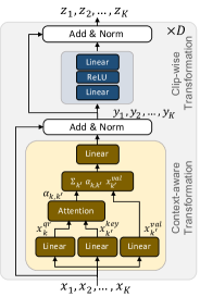
Figure 2: Architecture overview for contrastive audio-visual spatial alignment.

Figure 3: Transformer architecture for context-aware video-to-audio and audio-to-video feature translation.

3.2 Architecture

Figure 3 summarizes the architecture used to solve the spatial alignment task. First, video and audio encoders, $f_{v}$ and $f_{a}$, extract feature representations from each clip independently,

$$\mathbf{v}_{i}^{k}=f_{v}(v_{i}^{k})\mbox{\quad and\quad}\mathbf{a}_{i}^{k}=f_{a}(a_{i}^{k}).$$ (2)

These representations are then converted between the two modalities using audio-to-video $g_{a2v}$ and video-to-audio $g_{v2a}$ feature translation networks

$$\bar{\mathbf{v}}_{i}^{1},\ldots,\bar{\mathbf{v}}_{i}^{K}=g_{a2v}(\mathbf{a}_{i}^{1},\ldots,\mathbf{a}_{i}^{K})\mbox{\quad and\quad}\bar{\mathbf{a}}_{i}^{1},\ldots,\bar{\mathbf{a}}_{i}^{K}=g_{v2a}(\mathbf{v}_{i}^{1},\ldots,\mathbf{v}_{i}^{K}).$$ (3)

One important distinction between audio and video is the spatial localization of the signals. Unlike video, any sound source can be heard regardless of the listening angle. In other words, while an audio clip $a_{i}^{k}$ sampled at position $(\theta_{k},\phi_{k})$ contains audio from all sound sources present in a scene, only those physically located around $(\theta_{k},\phi_{k})$ can be seen on the video clip $v_{i}^{k}$. This implies that, to enable accurate feature translation, networks $g_{v2a}$ and $g_{a2v}$ should combine features from all sampled locations. This is accomplished by using a translation network similar to the transformer of [58]. As shown in Fig. 3, given a set of $K$ features $\{\mathbf{x}_{k}\}_{k=1}^{K}$, a transformer of depth $D$ alternates $D$ times between two modules. The first module combines the $K$ features $\mathbf{x}_{k}$ using attention

$$\alpha_{k,1},\ldots,\alpha_{k,K} = \mbox{\it Softmax}\left(\tfrac{\left\langle W_{key}^{T}\mathbf{x}_{k},W_{qr}^{T}\mathbf{x}_{1}\right\rangle}{\sqrt{d}},\ldots,\tfrac{\left\langle W_{key}^{T}\mathbf{x}_{k},W_{qr}^{T}\mathbf{x}_{K}\right\rangle}{\sqrt{d}}\right)$$ (4)

$$\mathbf{y}_{k} = \mbox{\it Norm}\left(\mathbf{x}_{k}+W_{0}^{T}\textstyle\sum_{k^{{}^{\prime}}}\alpha_{k,k^{{}^{\prime}}}W_{val}^{T}\mathbf{x}_{k^{{}^{\prime}}}\right).$$ (5)

The second module computes a simple clip-wise feed-forward transformation

$$\mathbf{z}_{k} = \mbox{\it Norm}\left(\mathbf{y}_{k}+W_{2}^{T}\max(W_{1}^{T}\mathbf{y}_{k},0)\right).$$ (6)

In (4)-(6), $W_{key},W_{qr},W_{val},W_{0},W_{1}$ and $W_{2}$ are learnable weights and Norm is layer normalization [6]. We omit the biases of linear transformations and layer indices for simplicity of notation. Compared to the original transformer [58], the proposed translation network differs in two aspects. First, motivated by early empirical results which showed no improvements on downstream tasks when utilizing multi-head attention, we simplified the transformer architecture to rely on a single attention head. Second, we removed positional encodings which are used to indicate the position of each token $\mathbf{x}_{k}$. While these encodings could be used to encode the viewing direction $(\theta_{k},\phi_{k})$ of each clip, doing so would allow the model to solve the spatial alignment task without learning semantic representations.

3.3 Learning strategy

AVSA is a difficult task to optimize since it requires discriminating between various crops from the same video. To enhance learning, we employed a curriculum learning strategy [7]. In the first phase, the network is trained to identify audio-visual correspondences (AVC) [3, 42] at the video level. This is accomplished by extracting a single crop $(v_{i},a_{i})$ for each video $i$ from a randomly drawn viewing angle. The visual and audio encoders, $f_{v}$ and $f_{a}$, are then trained to minimize

$$L_{\mbox{\it AVC}}=\sum_{i}L_{\mbox{\it InfoNCE}}\left(\mathbf{v}_{i},\mathbf{a}_{i},\left\{\mathbf{a}_{j}\right\}_{j=1}^{N}\right)+L_{\mbox{\it InfoNCE}}\left(\mathbf{a}_{i},\mathbf{v}_{i},\left\{\mathbf{v}_{j}\right\}_{j=1}^{N}\right)$$ (7)

where $\mathbf{v}_{i}=f_{v}(v_{i})$ and $\mathbf{a}_{i}=f_{a}(a_{i})$ are the video and audio representations. $L_{\mbox{\it InfoNCE}}$ is the InfoNCE loss [46] defined as

$$L_{\mbox{\it InfoNCE}}(\mathbf{x},\mathbf{x}_{t},\mathcal{P}_{\mathbf{x}})=-\log\cfrac{\exp(h(\mathbf{x}_{t},\mathbf{x})/\tau)}{\sum_{\mathbf{x}_{p}\in\mathcal{P}_{\mathbf{x}}}\exp(h(\mathbf{x}_{p},\mathbf{x})/\tau)}$$ (8)

where $h(\mathbf{x},\mathbf{x}_{t})$ is a prediction head that computes the cosine similarity between $\mathbf{x}$ and $\mathbf{x}_{t}$ after linear projection into a low-dimensional space, and $\tau$ is a temperature hyper-parameter. In the case of AVC, the target representation $\mathbf{x}_{t}$ for the InfoNCE loss is the feature from the crop of same video but opposing modality, and the proposal distribution $\mathcal{P}_{\mathbf{x}}$ is composed by the target feature representations of all videos in the batch.

In the second phase, the network is trained on the more challenging task of matching audio and video at the crop level, i.e. matching representations in the presence of multiple crops per video. This is accomplished by augmenting the proposal set $\mathcal{P}_{\mathbf{x}}$ to include representations from multiple randomly sampled viewing angles $\{(v_{i}^{k},a_{i}^{k})\}_{k=1}^{K}$ from the same video. In this phase, we also introduce the feature translation networks $g_{v2a}$ and $g_{a2v}$ and require the translated features ($\bar{\mathbf{v}}_{i}^{k}$ and $\bar{\mathbf{a}}_{i}^{k}$) to match the encoder outputs ($\mathbf{v}_{i}^{k}$ and $\mathbf{a}_{i}^{k}$) obtained for the corresponding viewing angle $k$. Encoders $f_{v}$ and $f_{a}$ and feature translation networks $g_{v2a}$ and $g_{a2v}$ are jointly trained to minimize

$$L_{\mbox{\it AVSA}}=\sum_{i}\sum_{k}L_{\mbox{\it InfoNCE}}\left(\bar{\mathbf{v}}_{i}^{k},\mathbf{v}_{i}^{k},\left\{\mathbf{v}_{j}^{l}\right\}_{j,l=1}^{N,K}\right)+L_{\mbox{\it InfoNCE}}\left(\bar{\mathbf{a}}_{i}^{k},\mathbf{a}_{i}^{k},\left\{\mathbf{a}_{j}^{l}\right\}_{j,l=1}^{N,K}\right).$$ (9)

4 YouTube-360 dataset

We collected a dataset of 360°video with spatial audio from YouTube, containing clips from a diverse set of topics such as musical performances, vlogs, sports, and others. This diversity is critical to learn good representations. Similarly to prior work [41], search results were cleaned by removing videos that 1) did not contain valid ambisonics, 2) only contain still images, or 3) contain a significant amount of post-production sounds such as voice-overs and background music. The resulting dataset, denoted YouTube-360 (YT-360), contains a total of 5 506 videos, which was split into 4 506 videos for training and 1 000 for testing. Since we use audio as target for representation learning, periods of silence were ignored. This was accomplished by extracting short non-overlapping clips whose volume level is above a certain threshold. In total, 88 733 clips of roughly 10s each were collected (246 hours of video content). As shown in fig. 5, the YT-360 dataset contains five times more videos than the largest 360°video dataset previously collected.

To assess the ability of AVSA pre-training to localize objects in a scene, we conduct evaluations on semantic segmentation as a downstream task. Due to the large size of our dataset, collecting ground-truth annotations is impractical. Instead, we used the state-of-the-art ResNet101 Panoptic FPN model [30] trained on the MS-COCO dataset [38] to segment the 32 most frequent objects and background classes on YT-360. A description of the segmentation procedure, including the selected classes, is provided in appendix. These segmentation maps are used to evaluate AVSA representations by knowledge distillation, as discussed in Section 5.3. Examples from the YT-360 dataset are shown in fig. 5 together with the predicted segmentation maps and a heat-map representing the directions of higher audio volume.

table[.4][][t] Spatial Audio Unique Videos Hours Duanmu et al. [13] 12 0.3 Li et al. [36] 73 3.8 Pano2VID [55] 86 7.3 SptAudioGen [41] ✓ 1146 113 YT-360 ✓ 5506 246 figure[.55][][t] Frames Audio energy Segmentation maps

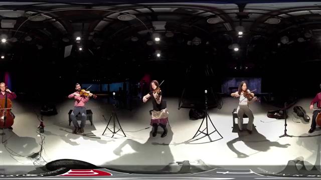
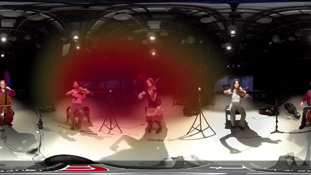
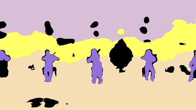
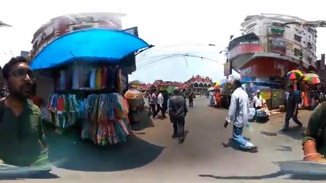
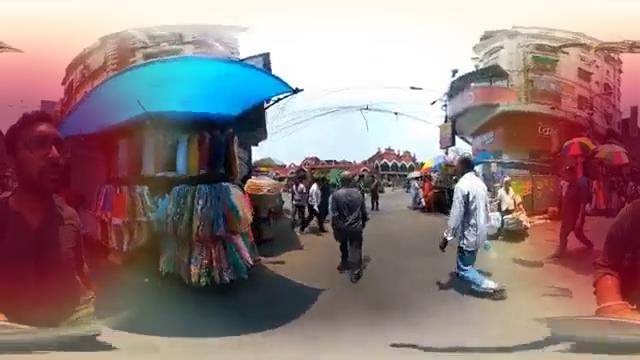
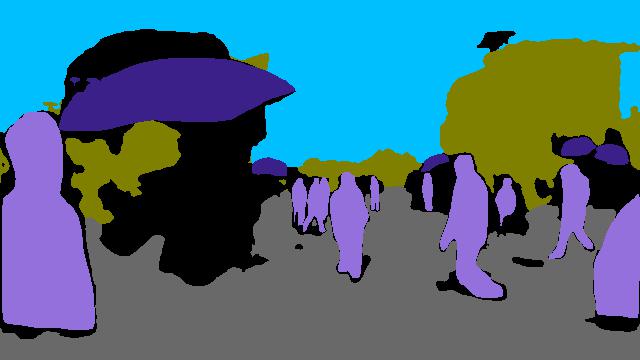
Figure 4: Comparison of 360°video datasets.

Figure 5: Examples from Youtube-360 dataset.

5 Experiments

We evaluate the representations learned by AVSA pre-training on several downstream tasks. We explain the experimental setting below, and refer the reader to appendix for additional details.

5.1 Experimental setting

Video pre-processing

We sampled $K=4$ crops per video at different viewing angles. Since up and down viewing directions are often less informative, we restrict the center of each crop to latitudes $\phi\in\{-60\degree,60\degree\}$. We also ensure that viewing angles are sampled at least 36°apart. Normal field-of-view (NFOV) crops are extracted using a Gnomonic projection with random angular coverage between 25°and 90°wide for data augmentation. If naive equi-rectangular crops were taken, the distortion patterns of these crops at latitudes outside the horizon line could potentially reveal the vertical position of the crop, allowing the network to “cheat” the AVSA task. Following NFOV projection, video clips are resized into $112\times 112$ resolution. Random horizontal flipping, color jittering and Z normalization are applied. Each video clip is $0.5s$ long and is extracted at 16fps.

Audio pre-processing

First-order ambisonics (FOA) are used for spatial audio. Audio clips for the different viewing angles are generated by simply rotating the ambisonics [32]. One second of audio is extracted at 24kHz, and four channels (FOA) of normalized log mel-spectrograms are used as the input to the audio encoder. Spectrograms are computed using an STFT with a window of size 21ms, and hop size of 10ms. The extracted frequency components are aggregated in a mel-scale with 128 levels.

Architecture and optimization

The video encoder $f_{v}$ is the 18-layer R2+1D model [57], and the audio encoder $f_{a}$ is a 9-layer 2D convolutional neural network operating on the time-frequency domain. The translation networks, $g_{v2a}$ and $g_{a2v}$, are instantiated with depth $D=2$. Training is conducted using the Adam optimizer [29] with a batch size of 28 distributed over 2 GPUs, learning rate of $1e-4$, weight decay of $1e-5$ and default momentum parameters $(\beta_{1},\beta_{2})=(0.9,0.999)$. Both curriculum learning phases are trained for 50 epochs. To control for the number of iterations, models trained only on the first or second phases are trained for 100 epochs.

Baseline pre-training methods

We compare AVSA to Audio-Visual Correspondence (AVC) [3, 4, 42] and Audio-Visual Temporal Synchronization (AVTS) [31, 47]. Since prior works perform pretext training on flat video datasets (i.e. without spatial audio), a direct comparison is impossible. Instead, we train AVC and AVTS models on the YouTube-360 dataset. For fair comparisons, we use the architecture and optimization settings described above. AVC is trained to optimize the loss of (7), which only uses negatives from different videos. Note that (7) is similar to the loss used in [3, 4] but considers multiple negatives simultaneously. This has actually been shown to improve generalization in [42]. To implement AVTS, we augment the proposal set $\mathcal{P}_{\mathbf{x}}$ of the InfoNCE loss of (8) with clips sampled from different moments in time. Following [31, 47], we ensure that negative pairs of audio and video clips are sufficiently separated in time. We also use a curriculum learning strategy composed by an AVC pre-training phase as in [31]. In the base AVC and AVTS implementations, we directly match the audio and visual features computed by the encoders $f_{v}$ and $f_{a}$ directly, as done in the original papers [3, 42, 31, 47]. However, to control for the number of seen crops, we also conduct AVC and AVTS pre-training using multiple crops of the same video and the feature translation networks $g_{a2v}$ and $g_{v2a}$. Since AVC requires predictions at the video level (not for each individual clip), clip representations are combined by max-pooling.

5.2 Audio-visual spatial alignment

We start by considering the performance on the AVC and AVSA tasks themselves. AVC performance is measured by randomly generating 50% of audio-video pairs from the same sample (positives), and 50% of pairs from different samples (negatives). Similarly, we designed a binary AVSA evaluation task in which positive audio-video pairs are spatially aligned, while negative pairs were artificially misaligned by randomly rotating the ambisonic audio of a positive pair. Rotations are constrained around the yaw axis (horizontal) to ensure the audio from positive and negative pairs have the same distribution, and thus making the AVSA task more challenging. Since models trained by AVC are not tuned for AVSA evaluation and vice-versa, the pretext models cannot be directly evaluated on the above binary tasks. Instead, we trained a new binary classification head on top of video and audio

Evaluation Task		AVC-Bin		AVSA-Bin
# Viewpoints		1	4	1	4
AVC	no transf.	79.82	82.68	59.48	59.25
	transf.	–	83.87	–	61.20
AVTS	no transf.	80.08	82.77	59.78	60.37
	transf.	–	83.77	–	60.73
AVSA	no transf.	86.19	91.67	64.97	68.87
	transf.	–	89.83	–	69.97

Table 1: Accuracy of binary AVC and AVSA predictions using one or four viewpoints on the YT-360 test set.

features, while keeping pretext representations frozen. Also, since NFOV video crops only cover a small portion of the 360°frame, we also consider predictions obtained by averaging over four viewpoints.

Table 1 shows that the proposed AVSA pretext training mechanism significantly outperforms AVC and AVTS on both evaluation tasks. Remarkably, even though AVC pretext training optimizes for the AVC task directly, representations learned with AVSA outperformed those learned with AVC by more than 6% on the AVC task itself (AVC-Bin). Furthermore, both AVC and AVTS models learned by audio-video correspondence or temporal synchronization do not transfer well to the spatial alignment task (AVSA-Bin). In result, AVSA outperforms AVC and AVTS by more than 5% on spatial alignment. By learning representations that are discriminative of different viewpoints, AVSA also learns a more diverse set of features. This is especially helpful when combining information from multiple viewpoints, as demonstrated by the differences in the gains obtained by 4 crop predictions. For example, AVC and AVTS only benefit by a 2-3% gain from 4 crop predictions on the AVC-Bin task, while AVSA performance improves by 5.5%. On the AVSA-Bin task, 4 crop predictions do not improve AVC or AVTS significantly, while AVSA performance still improves by 4%. We also observe improvements by using the transformer architecture in 5 out of 6 configurations (3 pretext tasks $\times$ 2 evaluations), showing its effectiveness at combining information from different viewpoints.

5.3 Semantic segmentation by knowledge distillation

AVSA representations are also evaluated on semantic segmentation. As shown in fig. 7, the video encoder $f_{v}$ was used to extract features at multiple scales, which were combined using a feature pyramid network (FPN) [37] for semantic segmentation. To measure the value added by audio inputs, we concatenate the features from the audio encoder $f_{a}$ at the start of the top-down pathway of the FPN head. Similarly, to measure the benefits of combining features from multiple viewpoints, we concatenate the context-aware representations computed by the feature translation modules $g_{v2a}$ and $g_{a2v}$. Since the goal is to evaluate the pretext representations, networks trained on the pretext task were kept frozen. The FPN head was trained by knowledge distillation, i.e. using the predictions of a state-of-the-art model as targets. We also compare to a fully supervised video encoder pre-trained on Kinetics for the task of action recognition. Similar to the self-supervised models, the fully supervised model was kept frozen. To provide an upper bound on the expected performance, we trained the whole system end-to-end (encoders, feature translation modules and the FPN head). A complete description of the FPN segmentation head and training procedure is given in appendix.

fig. 7 shows the pixel accuracy and mean IoU scores obtained using video features alone, or their combination with audio and context features. Examples of segmentation maps obtained with the AVSA model with context features are also shown in fig. 8. The results support several observations. AVSA learns significantly better visual features for semantic segmentation than AVC. This is likely due to the fine-grained nature of the AVSA task which requires discrimination of multiple crops within the same video frame. As a result, AVSA improves the most upon AVC on background classes such as rocks (34.7% accuracy vs. 27.7%), window (46.0% vs. 41.2%), pavement (36.8% vs. 33.3%), sand (42.1% vs. 38.8%), sea (50.1% vs. 46.8%) and road (47.1% vs. 45.1%).

AVSA also learns slightly better visual features than AVTS. While the gains over AVTS using visual features alone are smaller, AVTS cannot leverage the larger spatial context of 360°video data. When context features from four viewpoints are combined, using the translation networks $g_{v2a}$ and $g_{a2v}$, further improvements are obtained. With context features, AVSA yields a 3% mIoU improvement over AVC and 1% over AVTS.

Finally, we evaluated two ablations of AVSA. To verify the benefits of curriculum learning, we optimized the AVSA loss of (9) directly. Without curriculum, AVSA achieved 1.5% worse mIoU (see fig. 7 AVSA no curr.). We next verified the benefits of modeling spatial context by disabling the transformer ability to combine information from all viewpoints. This was accomplished by replacing the attention module of fig. 3 with a similarly sized multi-layer perceptron, which forced the translation networks to process each viewpoint independently. While this only produced slightly worse visual representations, the ability to leverage spatial context was significantly affected. Without the transformer architecture, AVSA yielded 1.5% worse mIoU scores when using context features (see fig. 7 AVSA mlp).

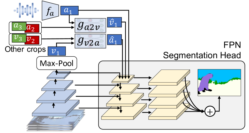
figure[.45][][c] table[.52][][c] Video only +Audio +Audio+Context Pix Acc mIoU Pix Acc mIoU Pix Acc mIoU AVC 71.16 32.85 71.07 32.69 – – AVTS 73.24 34.88 72.97 34.88 – – AVSA 73.44 35.11 73.11 34.63 73.85 35.83 AVSA (no curr.) 71.95 33.66 71.49 33.23 72.06 34.30 AVSA (mlp) 73.10 35.02 73.21 34.83 72.68 34.35 Kinetics (sup) 75.47 36.91 – – – – End-to-end (upper bound) 77.37 41.05 77.93 42.00 79.65 43.21

Figure 6: Architecture used for semantic segmentation. Pre-trained networks are kept frozen. A lightweight FPN segmentation head [37] is trained by knowledge distillation.

Figure 7: Pixel accuracy and mean IoU of semantic segmentation predictions on YT-360 test set. We evaluate the performance of an FPN head that uses 1) visual features alone, 2) visual and audio features, and 3) visual, audio and context features obtained from four viewpoints.

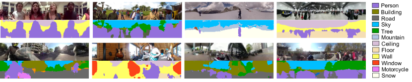
Figure 8: Predictions from an AVSA pre-trained model with an FPN segmentation head on the YT-360 test set.

5.4 Action recognition

	UCF		HMDB
	Clip@1	Video@1	Clip@1	Video@1
Scratch	54.85	59.95	27.40	31.10
Kinetics Sup.	78.50	83.43	46.45	51.90
AVC	64.63	69.68	31.33	34.58
AVTS	65.65	70.34	32.29	35.89
AVSA	68.52	73.80	32.96	37.66

Table 2: Action recognition performance on UCF and HMDB datasets. The top-1 accuracy of single clip and dense predictions are reported.

Action recognition is a common downstream task used to benchmark audio-visual self-supervised approaches. Following standard practices, we finetuned the pretext models either on the UCF [54] or the HMDB [33] datasets, and measure the top-1 accuracies obtained for a single clip or by averaging predictions over 25 clips per video. For comparison, we also provide the performance of our model trained on UCF and HMDB from a random initialization (Scratch), or finetuned from a fully supervised model trained on Kinetics [60] (Kinetics Sup.). Full details of the training procedure are given in appendix. The results shown in table 2 show once more the benefits of AVSA pretext training. AVSA dense predictions outperform AVC by 4% on UCF and 3% on HMDB, and outperform AVTS by 3.5% on UCF and 2% on HMDB.

6 Discussion, future work and limitations

We presented a novel self-supervised learning mechanism that leverages the spatial cues in audio and visual signals naturally occurring in the real world. Specifically, we collected a 360°video dataset with spatial audio, and trained a model to spatially align video and audio clips extracted from different viewing angles. The proposed AVSA task was shown to yield better representations than prior work on audio-visual self-supervision for downstream tasks like audio-visual correspondence, video semantic segmentation, and action recognition. We also proposed to model 360°video data as a collection of NFOV clips collected from multiple viewpoints, using a transformer architecture to combine view specific information. Being able to summarize information from the whole 360°video frame was proven advantageous for downstream tasks defined on 360°video data. For additional parametric and ablation studies, we refer the reader to supplementary material, where we ablate several components of the proposed approach, including the type of audio input provided to the network, the number and type of viewpoints in the AVSA objective, and the influence of curriculum learning and the transformer module.

Since AVSA requires discrimination of different viewpoints within a 360°scene, the learned models are encouraged to localize sound sources in the video and audio signals in order to match them. In addition to better performance on downstream tasks, this pre-training objective also translates into improved localization ability, based on a qualitative analysis. Fig. 9 shows several examples of GradCAM [51] visualizations for AVC and AVSA models (GradCAM is applied to each model’s audio-visual matching score). As can be seen, AVSA models tend to localize sound sources better. Furthermore, while the proposed method relies on randomly extracted video and audio clips, more sophisticated sampling techniques are an interesting direction of future work. For example, sampling can be guided towards objects using objectness scores, towards moving objects using optical flow, or towards sound sources by oversampling viewpoints with high audio energy. Such sampling techniques would better mimic a human learner, by actively choosing which parts of the environment to dedicate more attention. They would also under-sample less informative viewpoints (e.g. crops dominated by background), which are hard to match to the corresponding sound, and thus may harm the quality of learned representations.

Finally, we note that AVSA requires 360°data with spatial audio, which is still less prevalent than regular video. Previous methods, such as AVC and AVTS [3, 47, 31, 42], are often trained on datasets several orders of magnitude larger than YT-360, and can achieve better performance on downstream tasks such as action recognition. However, this work shows that, for the same amount of training data, AVSA improves the quality of the learned representations significantly. Due to the growing popularity of AR/VR, 360°content creation is likely to grow substantially. As the number of available 360°videos with spatial audio increases, the quality of representations learned by AVSA should improve as well.

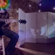
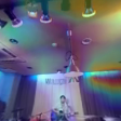
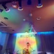
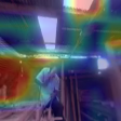
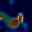
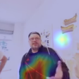
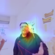
Figure 9: Sound localization maps (GradCAM of audio-visual matching scores) obtained from models trained by AVC (first image of each pair) and AVSA (second of each pair).

Broader Impact

Self-supervision reduces the need for human labeling, which is in some sense less affected by human biases. However, deep learning systems are trained from data. Thus, even self-supervised models reflect the biases in the collection process. To mitigate collection biases, we searched for 360°videos using queries translated into multiple languages. Despite these efforts, the adoption of 360°video cameras is likely not equal across different sectors of society, and thus learned representations may still reflect such discrepancies.

Appendix A Implementation details

In this section, we describe in detail the implementation of the proposed AVSA pre-training as well as the semantic segmentation and action recognition downstream tasks.

A.1 Audio-visual spatial alignment

The architecture of the video and audio encoder networks, $f_{v}$ and $f_{a}$, are shown in table 3. The feature translation networks are described in Section 3.2 and depicted in Figure 3 of the main text. These are transformer networks of base dimension 512 and expansion ration 4. In other words, the output dimensionality of the linear transformations of parameters $W_{key},W_{qr},W_{val},W_{0}$ and $W_{2}$ are 512, and that of $W_{1}$ is 2048. Models are pre-trained to optimize loss (7) for AVC task or (9) for AVTS and AVSA tasks. AVTS models are trained using negatives obtained from the same viewpoint but different moments in time. AVSA models are obtained using negatives obtained from the same moment in time but different viewpoints. All models were trained using the Adam optimized. Pre-training hyper-parameters are summarized in table 4.

A.2 Semantic segmentation

For semantic segmentation, we used a lightweight FPN segmentation head. As originally proposed, lateral connections are implemented with a $1\times{}1$ convolution that maps all feature maps into a 128 dimensional space followed by a $3\times{}3$ convolution for increased smoothing. Since the FPN head is used to perform semantic segmentation of a single frame given a video clip with multiple frames, we perform global temporal pooling of the feature maps before feeding them to the lateral connections. Semantic segmentation predictions are then computed based on the features at all levels. First, features from low-resolution layers are upsampled through a sequence of $3\times{}3$ convolutions with dilation of $2$ into $56\times{}56$ resolution and added together to perform pixel-wise classification. All parameters of the FPN head are trained to minimize the softmax cross-entropy loss average across all pixels. Since we are using the output of a state-of-the-art model as ground truth, we avoid using low-confidence ground-truth labels. Thus, all pixels for which the state-of-the-art model was less than 75% confident were kept unlabeled. These low confidence regions were also ignored while computing evaluation metrics. The model was trained using the Adam optimizer with batch size $20$, learning rate $1e-4$ and weight decay $5e-4$ for 10 epochs. The learning rate was decayed at epochs 5 and 8. Video clips were extracted from random viewpoints within the 360°video, with random angular coverage between 45°and 90°for data augmentation. Color jittering and horizontal flipping was also applied.

A.3 Action recognition

The video encoder network was evaluated on the task of action recognition using UCF and HMDB datasets. We augmented the video encoder with a linear classification layer after the global max-pooling operation, and finetune the whole network. We used Adam optimization for $100$ epochs, with batch size $28$, learning rate $10^{-4}$ decayed at epochs $40$, $60$ and $80$. Performance is reported on first train/test split originally defined for the UCF and HMDB datasets.

Appendix B Ablations and parametric studies

We assess different components of the proposed pre-trained mechanism through several ablation and parameteric studies shown in table 5. All models are evaluated on AVC-Bin, AVSA-Bin, semantic segmentation, and action recognition tasks as introduced in §5.2–5.4 of main text (4 crops per video are used for AVC-Bin and AVSA-Bin). We report accuracies for the AVC-Bin, AVSA-Bin tasks using 4 viewpoints, mean IoU for the semantic segmentation task and clip level accuracy for action recognition on UCF.

Influence of spatial audio

To demonstrate the value of spatial audio, we train the AVSA pretext task using different inputs to the audio network: single channel mono audio, two channel stereo audio, and four channel ambisonic audio. The three versions of the audio input can be easily computed from the full ambisonics signal. The mono version of audio is generated by taking the projection of the ambisonic signal into the spherical harmonics at each viewing angle. To generate stereo, we use a standard ambisonic binauralizer that models a human listener looking at each viewing angle. To generate ambisonics, we simply rotate the original signal to align with each viewing angle. Assuming a typical ambisonics format with 4 channels, this is done by applying a 3D rotation matrix to its first-order spherical harmonic components ($X$, $Y$ and $Z$ channels), while keeping the zeroth-order component ($W$ channel) fixed.

table 5(a) shows substantial improvement ($\sim 7\%$) in AVC and AVSA tasks by using full ambisonics for each crop over mono audio, suggesting that the latter may not be sufficient to encode spatial information of sound sources. Using stereo audio which retains partial spatial information also improves over mono input, but with a smaller margin. For semantic tasks (segmentation and action recognition on UCF), learning with ambisonics also proved to be more effective.

Influence of number of viewpoints

As more viewpoints are extracted from each sample, the difficulty of the AVSA task increases since more options are provided for matching. To investigate whether the increased difficulty correlates with the quality of the learned representation, we vary the number of viewpoints during AVSA pre-training.

table 5(b) shows the AVC and AVSA performance increases monotonically as more viewpoints are used. However, these gains not always translates into better performance on semantic tasks. Semantic segmentation achieved the best performance by training to discriminate 2 or 4 viewpoints, while action recognition peaked at 4 viewpoints.

Influence of type of negative crops

The AVSA pretext tasks uses a combination of easy and hard (spatial) negatives: Easy negatives are clips from different video instances. Hard (spatial) negatives are sampled from different viewpoints, but the same moment in time. We also trained a network with hard spatio-temporal negatives, which can be sampled from any viewpoint and moment in time within the video. table 5(c) shows the performance of models trained with different kinds of negatives crops. As can be seen, the combination of instance-based and spatial negatives (as used by the AVSA approach) yields better performance than using instance-based negatives alone (as used by AVC approaches). This shows the use of spatial negatives is complementary to AVC. However, the results are mixed when combining AVSA with temporal negatives (as used by AVTS approaches), producing slightly better semantic segmentations, but worse UCF performance.

Influence of curriculum learning

Prior work indicates that curriculum learning can benefit training by starting from easier sub-tasks and progressively increase the difficulty of the task being learned. To test this hypothesis in the AVSA context, we evaluate our network trained with and without the curriculum learning strategy (first optimizing for easy negatives, i.e. AVC, then optimizing for easy and hard negatives combined). We also compare to baselines where the model is only optimized for easy or hard negatives.

table 5(d) shows that training on hard negatives directly leads to the best AVC and AVSA performance. However, the learned representations significantly overfit to the pretext task, and do not transfer well to semantic tasks, as seen by the low performance on semantic segmentation and action recognition. Using a combination of easy and hard negatives proved to be beneficial for these two downstream tasks, with the curriculum learning strategy achieving the best results.

Influence of modeling spatial context

We propose to use a transformer network to leverage the rich spatial context of spatial audio and 360°video while translating features across the two modalities. To assess the importance of modeling spatial context, we evaluate models trained with and without the transformer networks. We further vary the depth of transformer module in search of a good trade-off between model complexity and quality of learned representations.

table 5(e) shows that modeling spatial context is not required to predict whether audio and video clips originate from the same sample (achieving lower AVC accuracy). However, the ability to perform spatial alignment is significantly impacted without the transformer network, showing that it is harder to perform spatial alignment without combining information from multiple viewpoints. The lack of spatial context also impacted both semantic segmentation and action recognition on UCF. For semantic tasks, a transformer of depth $D=2$ provided a good trade-off between model complexity and model performance.

Table 3: Architecture details of R(2+1)D video network and Conv2D audio network. The video network is based of R(2+1)D convolutions, and the audio on 2D convolutions. Both video and audio networks use ReLU activations and batch normalization at each layer. $X_{s}$ spatial activation size, $X_{t}$ temporal activation size, $X_{f}$ frequency activation size, $C$ number of channels, $K_{s}$ spatial kernel size, $K_{t}$ temporal kernel size, $K_{f}$ frequency kernel size, $S_{s}$ spatial stride, $S_{t}$ temporal stride, $S_{f}$ frequency stride. The input to the audio network is a $N$-channel spectrogram, where $N=1$ for experiments with mono audio, $N=2$ with stereo and $N=4$ with ambisonics.

Video Network
Layer	$X_{s}$	$X_{t}$	$C$	$K_{s}$	$K_{t}$	$S_{s}$	$S_{t}$
video	112	8	3	-	-	-	-
conv1	56	8	64	7	3	2	1
block2.1	56	8	64	3	3	1	1
	56	8	64	3	3	1	1
block2.2	56	8	64	3	3	1	1
	56	8	64	3	3	1	1
block3.1	28	4	128	3	3	2	2
	28	4	128	3	3	1	1
block3.2	28	4	128	3	3	1	1
	28	4	128	3	3	1	1
block4.1	14	2	256	3	3	2	2
	14	2	256	3	3	1	1
block4.2	14	2	256	3	3	1	1
	14	2	256	3	3	1	1
block5.1	7	1	512	3	3	2	2
	7	1	512	3	3	1	1
block5.2	7	1	512	3	3	1	1
	7	1	512	3	3	1	1
max pool	1	1	512	7	1	1	1

Audio Network
Layer	$X_{f}$	$X_{t}$	$C$	$K_{f}$	$K_{t}$	$S_{f}$	$S_{t}$
audio	129	100	$N$	-	-	-	-
conv1	65	50	64	7	7	2	2
block2.1	65	50	64	3	3	1	1
block2.2	65	50	64	3	3	1	1
block3.1	33	25	128	3	3	2	2
block3.2	33	25	128	3	3	1	1
block4.1	17	13	256	3	3	2	2
block4.2	17	13	256	3	3	1	1
block5.1	17	13	512	3	3	1	1
block5.2	17	13	512	3	3	1	1
max pool	1	1	512	17	13	1	1

Method

bs

nv

lr

wd

cj

hf

$\textrm{hfov}_{\textrm{min}}$

$\textrm{hfov}_{\textrm{max}}$

in

sn

tn

$\tau$

AVC

112

1

1e-4

1e-5

✓

0.5

25

90

✓

0.07

AVTS

28

4

1e-4

1e-5

✓

0.5

25

90

✓

✓

0.07

AVSA

28

4

1e-4

1e-5

✓

0.5

25

90

✓

✓

0.07

Table 4: Pre-training optimization hyper-parameters. AVSA models are initialized by the AVC model obtained at epoch 100. bs–batch size; nv–number of viewpoints; lr–learning rate; wd–weight decay; cj–color jittering; hf–horizontal flip probability; $\textrm{hfov}_{\textrm{min}}$/$\textrm{hfov}_{\textrm{max}}$–minimum/maximum horizontal field-of-view in degrees; in/sn/tn–instance/spatial/temporal negatives; $\tau$–InfoNCE temperature.

	AVC@4	AVSA@4	Segm	UCF
Mono	82.39	62.95	34.21	64.90
Stereo	84.47	71.11	34.54	64.68
Ambisonics	89.83	69.97	35.83	68.52

(a) Spatial audio format.

	AVC@4	AVSA@4	Segm	UCF
1 Viewpoint	84.60	61.77	35.37	64.71
2 Viewpoints	87.70	63.71	36.63	66.64
4 Viewpoints	89.83	69.97	35.83	68.52
8 Viewpoints	91.65	74.64	34.84	66.44

(b) Number of viewpoints.

	AVC@4	AVSA@4	Segm	UCF
Instance	83.87	61.20	34.05	64.09
+ Spatial	89.83	69.97	35.83	68.52
+ Spatial + Temporal	89.65	72.81	36.11	65.77

(c) Negative crop type.

	AVC@4	AVSA@4	Segm	UCF
Easy Only	83.87	61.20	34.05	64.09
Hard Only	93.22	77.71	20.97	59.15
No Curriculum	91.93	71.77	35.29	65.49
Curriculum	89.83	69.97	35.83	68.52

(d) Curriculum learning.

	AVC@4	AVSA@4	Segm	UCF
Direct Prediction	91.67	68.87	34.50	65.59
Transformer (Depth=1)	90.64	72.95	35.77	66.97
Transformer (Depth=2)	89.83	69.97	35.83	68.52
Transformer (Depth=4)	89.86	70.09	35.97	66.88

(e) Modeling spatial context.

Table 5: Ablation studies.

References

- [1] Alwassel, H., Mahajan, D., Torresani, L., Ghanem, B., Tran, D.: Self-supervised learning by cross-modal audio-video clustering. arXiv preprint arXiv:1911.12667 (2019)
- [2] Andersen, T.S., Tiippana, K., Sams, M.: Factors influencing audiovisual fission and fusion illusions. Cognitive Brain Research 21(3), 301–308 (2004)
- [3] Arandjelovic, R., Zisserman, A.: Look, listen and learn. In: International Conference on Computer Vision (ICCV) (2017)
- [4] Arandjelovic, R., Zisserman, A.: Objects that sound. In: European Conference on Computer Vision (ECCV) (2018)
- [5] Aytar, Y., Vondrick, C., Torralba, A.: Soundnet: Learning sound representations from unlabeled video. In: Advances in Neural Information Processing Systems (NeurIPS) (2016)
- [6] Ba, J.L., Kiros, J.R., Hinton, G.E.: Layer normalization. arXiv preprint arXiv:1607.06450 (2016)
- [7] Bengio, Y., Louradour, J., Collobert, R., Weston, J.: Curriculum learning. In: 26th annual international conference on machine learning. pp. 41–48 (2009)
- [8] Caron, M., Bojanowski, P., Joulin, A., Douze, M.: Deep clustering for unsupervised learning of visual features. In: European Conference on Computer Vision (ECCV) (2018)
- [9] Chen, T., Kornblith, S., Norouzi, M., Hinton, G.: A simple framework for contrastive learning of visual representations. arXiv preprint arXiv:2002.05709 (2020)
- [10] Cheng, H.T., Chao, C.H., Dong, J.D., Wen, H.K., Liu, T.L., Sun, M.: Cube padding for weakly-supervised saliency prediction in 360 videos. In: IEEE Conference on Computer Vision and Pattern Recognition. pp. 1420–1429 (2018)
- [11] Chung, J.S., Zisserman, A.: Out of time: automated lip sync in the wild. In: Asian Conference on Computer Vision (ACCV) (2016)
- [12] Doersch, C., Gupta, A., Efros, A.A.: Unsupervised visual representation learning by context prediction. In: International Conference on Computer Vision (ICCV) (2015)
- [13] Duanmu, F., Mao, Y., Liu, S., Srinivasan, S., Wang, Y.: A subjective study of viewer navigation behaviors when watching 360-degree videos on computers. In: 2018 IEEE International Conference on Multimedia and Expo (ICME). pp. 1–6. IEEE (2018)
- [14] Emberson, L.L., Richards, J.E., Aslin, R.N.: Top-down modulation in the infant brain: Learning-induced expectations rapidly affect the sensory cortex at 6 months. National Academy of Sciences 112(31), 9585–9590 (2015)
- [15] Gan, C., Huang, D., Zhao, H., Tenenbaum, J.B., Torralba, A.: Music gesture for visual sound separation. arXiv preprint arXiv:2004.09476 (2020)
- [16] Gao, R., Feris, R., Grauman, K.: Learning to separate object sounds by watching unlabeled video. In: European Conference on Computer Vision (ECCV) (2018)
- [17] Gao, R., Grauman, K.: 2.5d visual sound. In: IEEE Conference on Computer Vision and Pattern Recognition. pp. 324–333 (2019)
- [18] Gao, R., Grauman, K.: Co-separating sounds of visual objects. In: IEEE International Conference on Computer Vision. pp. 3879–3888 (2019)
- [19] Gerzon, M.A.: Periphony: With-height sound reproduction. Journal of the audio engineering society 21(1), 2–10 (1973)
- [20] Hadsell, R., Chopra, S., LeCun, Y.: Dimensionality reduction by learning an invariant mapping. In: IEEE Conference on Computer Vision and Pattern Recognition (CVPR) (2006)
- [21] Han, T., Xie, W., Zisserman, A.: Video representation learning by dense predictive coding. In: Workshop on Large Scale Holistic Video Understanding, ICCV (2019)
- [22] Harwath, D., Torralba, A., Glass, J.: Unsupervised learning of spoken language with visual context. In: Advances in Neural Information Processing Systems (NeurIPS) (2016)
- [23] He, K., Fan, H., Wu, Y., Xie, S., Girshick, R.: Momentum contrast for unsupervised visual representation learning. arXiv preprint arXiv:1911.05722 (2019)
- [24] Ho, C.H., Vasconcelos, N.: Contrastive learning with adversarial examples. In: Advances in Neural Information Processing Systems (NeurIPS) (2020)
- [25] Hu, H.N., Lin, Y.C., Liu, M.Y., Cheng, H.T., Chang, Y.J., Sun, M.: Deep 360 pilot: Learning a deep agent for piloting through 360 sports videos. In: 2017 IEEE Conference on Computer Vision and Pattern Recognition (CVPR). pp. 1396–1405. IEEE (2017)
- [26] Ji, X., Henriques, J.F., Vedaldi, A.: Invariant information distillation for unsupervised image segmentation and clustering. arXiv preprint arXiv:1807.06653 (2018)
- [27] Jiang, H., Larsson, G., Maire Greg Shakhnarovich, M., Learned-Miller, E.: Self-supervised relative depth learning for urban scene understanding. In: European Conference on Computer Vision (ECCV) (2018)
- [28] Kim, D., Cho, D., Kweon, I.S.: Self-supervised video representation learning with space-time cubic puzzles. In: AAAI Conference on Artificial Intelligence (2019)
- [29] Kingma, D.P., Ba, J.: Adam: A method for stochastic optimization. arXiv preprint arXiv:1412.6980 (2014)
- [30] Kirillov, A., He, K., Girshick, R., Rother, C., Dollár, P.: Panoptic segmentation. In: IEEE conference on computer vision and pattern recognition. pp. 9404–9413 (2019)
- [31] Korbar, B., Tran, D., Torresani, L.: Cooperative learning of audio and video models from self-supervised synchronization. In: Advances in Neural Information Processing Systems (NeurIPS) (2018)
- [32] Kronlachner, M., Zotter, F.: Spatial transformations for the enhancement of ambisonic recordings. In: 2nd International Conference on Spatial Audio, Erlangen (2014)
- [33] Kuehne, H., Jhuang, H., Garrote, E., Poggio, T., Serre, T.: HMDB: a large video database for human motion recognition. In: 2011 International Conference on Computer Vision (ICCV). IEEE (2011)
- [34] Payen de La Garanderie, G., Atapour Abarghouei, A., Breckon, T.P.: Eliminating the blind spot: Adapting 3d object detection and monocular depth estimation to 360 panoramic imagery. In: European Conference on Computer Vision (ECCV). pp. 789–807 (2018)
- [35] Lee, H., Battle, A., Raina, R., Ng, A.Y.: Efficient sparse coding algorithms. In: Advances in Neural Information Processing Systems (NeurIPS) (2007)
- [36] Li, B.J., Bailenson, J.N., Pines, A., Greenleaf, W.J., Williams, L.M.: A public database of immersive vr videos with corresponding ratings of arousal, valence, and correlations between head movements and self report measures. Frontiers in psychology 8, 2116 (2017)
- [37] Lin, T.Y., Dollár, P., Girshick, R., He, K., Hariharan, B., Belongie, S.: Feature pyramid networks for object detection. In: IEEE conference on computer vision and pattern recognition. pp. 2117–2125 (2017)
- [38] Lin, T.Y., Maire, M., Belongie, S., Hays, J., Perona, P., Ramanan, D., Dollár, P., Zitnick, C.L.: Microsoft coco: Common objects in context. In: European Conference on Computer Vision (ECCV) (2014)
- [39] McGurk, H., MacDonald, J.: Hearing lips and seeing voices. Nature 264(5588), 746–748 (1976)
- [40] Misra, I., van der Maaten, L.: Self-supervised learning of pretext-invariant representations. In: IEEE Conference on Computer Vision and Pattern Recognition (CVPR) (2020)
- [41] Morgado, P., Vasconcelos, N., Langlois, T., Wang, O.: Self-supervised generation of spatial audio for 360 video. In: Advances in Neural Information Processing Systems (NeurIPS) (2018)
- [42] Morgado, P., Vasconcelos, N., Misra, I.: Audio-visual instance discrimination with cross-modal agreement. arXiv preprint arXiv:2004.12943 (2020)
- [43] Noroozi, M., Favaro, P.: Unsupervised learning of visual representations by solving jigsaw puzzles. In: European Conference on Computer Vision (ECCV) (2016)
- [44] Olshausen, B.A.: Sparse coding of time-varying natural images. In: Proc. of the Int. Conf. on Independent Component Analysis and Blind Source Separation (2000)
- [45] Olshausen, B.A., Field, D.J.: Emergence of simple-cell receptive field properties by learning a sparse code for natural images. Nature 381(6583), 607 (1996)
- [46] Oord, A.v.d., Li, Y., Vinyals, O.: Representation learning with contrastive predictive coding. arXiv preprint arXiv:1807.03748 (2018)
- [47] Owens, A., Efros, A.A.: Audio-visual scene analysis with self-supervised multisensory features. In: European Conference on Computer Vision (ECCV) (2018)
- [48] Owens, A., Wu, J., McDermott, J.H., Freeman, W.T., Torralba, A.: Ambient sound provides supervision for visual learning. In: European Conference on Computer Vision (ECCV) (2016)
- [49] Ranzato, M., Huang, F.J., Boureau, Y.L., LeCun, Y.: Unsupervised learning of invariant feature hierarchies with applications to object recognition. In: IEEE Conference on Computer Vision and Pattern Recognition (CVPR) (2007)
- [50] de Sa, V.R.: Learning classification with unlabeled data. In: Advances in Neural Information Processing Systems (NeurIPS) (1994)
- [51] Selvaraju, R.R., Cogswell, M., Das, A., Vedantam, R., Parikh, D., Batra, D.: Grad-cam: Visual explanations from deep networks via gradient-based localization. In: IEEE international conference on computer vision. pp. 618–626 (2017)
- [52] Senocak, A., Oh, T.H., Kim, J., Yang, M.H., So Kweon, I.: Learning to localize sound source in visual scenes. In: IEEE Conference on Computer Vision and Pattern Recognition (CVPR) (2018)
- [53] Shams, L., Kamitani, Y., Shimojo, S.: What you see is what you hear. Nature 408(6814), 788–788 (2000)
- [54] Soomro, K., Zamir, A.R., Shah, M.: UCF101: A dataset of 101 human actions classes from videos in the wild. Tech. Rep. CRCV-TR-12-01 (2012)
- [55] Su, Y.C., Jayaraman, D., Grauman, K.: Pano2vid: Automatic cinematography for watching 360°videos. In: Asian Conference on Computer Vision (ACCV) (2016)
- [56] Tian, Y., Krishnan, D., Isola, P.: Contrastive multiview coding. In: Workshop on Self-Supervised Learning, ICML (2019)
- [57] Tran, D., Wang, H., Torresani, L., Ray, J., LeCun, Y., Paluri, M.: A closer look at spatiotemporal convolutions for action recognition. In: IEEE Conference on Computer Vision and Pattern Recognition (CVPR) (2018)
- [58] Vaswani, A., Shazeer, N., Parmar, N., Uszkoreit, J., Jones, L., Gomez, A.N., Kaiser, Ł., Polosukhin, I.: Attention is all you need. In: Advances in neural information processing systems. pp. 5998–6008 (2017)
- [59] Vetter, P., Smith, F.W., Muckli, L.: Decoding sound and imagery content in early visual cortex. Current Biology 24(11), 1256–1262 (2014)
- [60] W. Kay, J. Carreira, K. Simonyan, B. Zhang, C. Hillier, S. Vijayanarasimhan, F. Viola, T. Green, T. Back, P. Natsev, M. Suleyman, and A. Zisserman: The kinetics human action video dataset. arXiv:1705.06950 (2017)
- [61] Wang, F.E., Hu, H.N., Cheng, H.T., Lin, J.T., Yang, S.T., Shih, M.L., Chu, H.K., Sun, M.: Self-supervised learning of depth and camera motion from 360°videos. In: Asian Conference on Computer Vision. pp. 53–68. Springer (2018)
- [62] Weisstein, E.W.: Gnomonic projection. From MathWorld–A Wolfram Web Resource. http://mathworld. wolfram. com/GnomonicProjection. html (2020)
- [63] Wu, Z., Xiong, Y., Yu, S.X., Lin, D.: Unsupervised feature learning via non-parametric instance discrimination. In: IEEE Conference on Computer Vision and Pattern Recognition (CVPR) (2018)
- [64] Xiao, J., Ehinger, K.A., Oliva, A., Torralba, A.: Recognizing scene viewpoint using panoramic place representation. In: 2012 IEEE Conference on Computer Vision and Pattern Recognition. pp. 2695–2702. IEEE (2012)
- [65] Zhang, R., Isola, P., Efros, A.A.: Split-brain autoencoders: Unsupervised learning by cross-channel prediction. In: IEEE Conference on Computer Vision and Pattern Recognition (CVPR) (2017)
- [66] Zhang, Z., Xu, Y., Yu, J., Gao, S.: Saliency detection in 360 videos. In: European Conference on Computer Vision (ECCV). pp. 488–503 (2018)
- [67] Zhao, H., Gan, C., Ma, W.C., Torralba, A.: The sound of motions. In: IEEE International Conference on Computer Vision. pp. 1735–1744 (2019)
- [68] Zhao, H., Gan, C., Rouditchenko, A., Vondrick, C., McDermott, J., Torralba, A.: The sound of pixels. In: European Conference on Computer Vision (ECCV) (2018)