Floquet Engineering of a Dynamical $Z_{2}$ Lattice Gauge Field with Ultracold Atoms

Abstract

In this paper, we propose that a simple model, in which fermions coupled to a dynamical lattice gauge field, can be engineered via the Floquet approach. The model possess both a independent Maxwell term and the local $Z_{2}$ gauge symmetry. Our proposal relies on a species dependent optical lattice, and can be achieved in one, two or three dimension. By an unitary transformation, this model can be mapped into a non-interacting composite Fermion system with fluctuating back ground charge. With the help of this composite Fermion picture, two characteristic observations are predicted. One is the radio-frequency spectroscopy, which exhibits no dispersion in all parameter regimes. Second is the the dynamical localization, which depends on the structure of the initial states.

The Gauge field theory is one of the most important footing stone of the modern physics. On one hand, the gauge theory successfully described the fundamental interactions within the standard model of high energy physics. On another hand, lattice gauge theory can also emerges from the low-energy physics of the strongly correlated systems Rev@Kogut.1979 . For example, the $U(1)$ lattice gauge theory can effectively describe the collective fluctuations of the frustrated magnetism fru_mag@Balents.2010 ; fru_mag@Read.1991 ; fru_mag@Sachdev.1991 , quantum spin liquid SL@Anderson.1988 ; SL@Read.1988 ; SL@Affleck.1988 ; SL@Fisher.2000 , quantum dimer model QDM@Kivelson.1987 ; QDM@Fradkin.2001 . In fact, dynamical gauge fields entre the theory naturally in the so-called slave-particle decomposition, whereby the original particles are fractionalized into slave degrees of freedom. The relative phase between the slave particles introduces the local gauge invariance. Understanding the real time dynamics of lattice gauge fields is a notable challenge due to the limit of the classical computational methods. This stimulates the efforts on the quantum simulation of the gauge fields in various engineered systems  U1EXP@Zoller.2016 ; U1EXP@Yuan.2020 ; U1EXP@Jendrzejewski.2020 . LGT_REV@Wiese.2013 ; LGT_CAP@Demler.2018 ; LGT@Grover.2016 ; Z2@Cirac.2017

In cold atom system, static artificial gauge fields has been simulated in recent years, including electrical field Electric@Spielman.2011 , magnetic field Magnetic@Spielman.2009 , and even spin-orbit couplings SOC@Spielman.2011 ; 2DSOC@Chen.Shuai.2016 . However the configuration of those gauge fields is fixed by the external laser or the system geometry. Therefore these fields have no dynamics, and can not mediate the interaction between atoms. Recently, Chicago and ETH group have realized the density-dependent gauge field by periodic modulation of the optical lattice or the interaction DDGF@Chin.2018 ; DDGF@Esslinger.2019 ; while Stanford group has realized a cavity-induced one dimensional spin-orbit-coupled Bose-Einstein condensate Cavity_SOC@Lev.2019 . In these experiments, the artificial gauge fields are no longer static, but can fluctuate with time. However the local gauge invariance, the key ingredient of the gauge theory, is still missing. In 2019, Bloch’s group successfully simulated the dynamical $Z_{2}$ lattice gauge field in a double well potential Z2EXP@Bloch.2019 , where the coupled dynamics of a single boson and the gauge field are observed.

In this paper, inspired by the Bloch’s experiment, we propose that a simplest model, in which fermions interacting with a dynamical lattice gauge field with local $Z_{2}$ invariant, can be engineered via the Floquet approach. Our setup can be applied in one, two or three dimension. By an unitary transformation, this model can be mapped into a non-interacting composite Fermion system with fluctuating back ground charge. With the help of this composite Fermion picture, two characteristic observations are predicted. One is that the radio-frequency spectrum of the Fermions exhibits no dispersion in all parameter regimes, which reflects the local symmetry of the model. Second is the dynamical localization of the Fermions, which depends on the structure of the initial states.

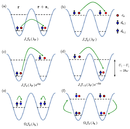
Figure 1: The physical processes keeped in effective Hamiltonian. Red circles represent the spinless $\hat{c}$-fermions hopping in the lattice; while blue circles with arrow represent the spinful localized $\hat{d}$-fermions. (a)(b) The renormalized hopping of $\hat{c}$-fermions in the case of same spins polarize of $\hat{d}$-fermions between the neighbor sites. (c)(d) The shaking assistant hopping of $\hat{c}$-fermions in the case of opposite spin polarizations of $\hat{d}$-fermions. (e) The renormalized spin flip of $\hat{d}$-fermions in the absence of $\hat{c}$-fermions. (f) The shaking assistant spin flip of $\hat{d}$-fermions in the presence of $\hat{c}$-fermions.

Experiment setup. We consider two kinds of atoms, one is mobile spinless fermion noted by $\hat{c}_{\mathbf{r}}$, which is used to simulate the matter field; while another is localized spin-$1/2$ fermions noted by $\hat{d}_{\mathbf{r,\uparrow(\downarrow)}}$ to simulate the gauge field. The fermions are trapped in a species dependent cubic optical lattice. By carefully tuning the optical lattice, one can highly suppress the hopping of the $\hat{d}$-fermions; while keeping the hopping of the $\hat{c}$-fermions. An radio-frequency field is applied to coupled spin up and spin down states of the $\hat{d}$-fermions. The tight-binding Hamiltonian reads $\hat{H}(t)=\hat{H}_{0}+\hat{H}_{\mathrm{I}}+\hat{V}(t)$, where

$$H_{0} = J\sum\limits_{\mathbf{r,}i}\hat{c}_{\mathbf{r}+\mathbf{a}_{i}}^{{\dagger}}\hat{c}_{\mathbf{r}}+\Omega\sum\limits_{\mathbf{r}}\hat{d}_{\mathbf{r,\uparrow}}^{{\dagger}}\hat{d}_{\mathbf{r,\downarrow}}+h.c.,$$ (1)

$$\hat{H}_{\mathrm{I}} = \sum\limits_{\mathbf{r}}(U_{\uparrow}\hat{n}_{\mathbf{r,\uparrow}}^{d}\hat{n}_{\mathbf{r}}^{c}+U_{\downarrow}\hat{n}_{\mathbf{r,\downarrow}}^{d}\hat{n}_{\mathbf{r}}^{c}),$$ (2)

$$\hat{V}(t) = \sum\limits_{\mathbf{r}}\left[\mathbf{F}(t)\mathbf{\cdot r}\hat{n}_{\mathbf{r}}^{c}+h(t)(\hat{n}_{\mathbf{r,\uparrow}}^{d}-\hat{n}_{\mathbf{r,\downarrow}}^{d})\right].$$ (3)

Here $\mathbf{a}_{i}=a\mathbf{e}_{i}$, is the basic vector of the cubic lattice, $U_{\uparrow(\downarrow)}$ is the on-site interaction between the $\hat{c}$-fermions and spin up (down) $\hat{d}$-fermions. The interaction between the spin-up and spin-down $\hat{d}$-fermions is irrelevant in this problem, since we constrain the particle number of $\hat{d}$-fermion at each site to be unit, $\hat{n}_{\mathbf{r,\uparrow}}^{d}+\hat{n}_{\mathbf{r,\downarrow}}^{d}=1$. There are two periodic driving term. One is an oscillating Zeeman field, $h(t)=h\cos(\omega t)$, which is applied on the $\hat{d}$-fermions. Another is an periodic driving force, $\mathbf{F}(t)=F\cos(\omega t+\phi)\sum\limits_{i=1}^{3}\mathbf{e}_{i}$, which can be realized by linear polarized shaking of the optical lattice. The two driving terms have the same frequency with a phase shift $\phi$. We choose the driving frequency to be two-photon resonance with the interaction difference $2\hbar\omega=U_{\uparrow}-U_{\downarrow}$, and the phase shift to be $\phi=\pi/2$.

To deal with this time periodic driven quantum system, we first make a rotating transformation, $\hat{R}(t)=\exp\left\{-\frac{i}{\hbar}\int\nolimits_{0}^{t}d\tau[\hat{H}_{\mathrm{I}}+\hat{V}(\tau)]\right\},$ to eliminate the interaction and the driving terms. One obtains the Hamiltonian in the rotating frame as

$$\hat{H}_{\mathrm{rw}}(t) = J\sum\limits_{\mathbf{r,}i}\hat{c}_{\mathbf{r}+\mathbf{a}_{i}}^{{\dagger}}\hat{P}_{\mathbf{r}+\mathbf{a}_{i}}^{d}\hat{P}_{\mathbf{r}}^{d}\hat{c}_{\mathbf{r}}e^{i\frac{Fa}{\hbar\omega}\sin(\omega t)}+$$ (4)

$$\Omega\sum\limits_{\mathbf{r}}\hat{d}_{\mathbf{r,\uparrow}}^{{\dagger}}\hat{P}_{\mathbf{r,\uparrow}}^{c}\hat{P}_{\mathbf{r,\uparrow}}^{c}\hat{d}_{\mathbf{r,\downarrow}}e^{i\frac{2h}{\hbar\omega}\cos(\omega t)}+h.c.,$$

where $\hat{P}_{\mathbf{r}}^{d}=\hat{n}_{\mathbf{r,\uparrow}}^{d}e^{-iU_{\uparrow}t/\hbar}+\hat{n}_{\mathbf{r,\downarrow}}^{d}e^{-iU_{\downarrow}t/\hbar}$, and $\hat{P}_{\mathbf{r,\uparrow}\left(\mathbf{\downarrow}\right)}^{c}=(1-\hat{n}_{\mathbf{r}}^{c})+\hat{n}_{\mathbf{r}}^{c}e^{-iU_{\mathbf{\uparrow}\left(\downarrow\right)}t/\hbar}$ are oscillating phase factors, depending on the occupation of $\hat{d}$-fermion and $\hat{c}$-fermions respectively.

Then we apply the high frequency expansion to seek the time independent effective Hamiltonian as $\hat{H}_{\mathrm{eff}}=\hat{H}_{\mathrm{rw}}^{(0)}+\sum_{m=1}^{\infty}\frac{\left[\hat{H}_{\mathrm{rw}}^{(m)},\hat{H}_{\mathrm{rw}}^{(-m)}\right]}{m\hbar\omega}+\cdots$, where $\hat{H}_{\mathrm{rw}}^{(m)}=\frac{1}{T}\int\nolimits_{0}^{T}dt\hat{H}_{\mathrm{rw}}(t)e^{-im\omega t}$ is the Fourier component of the Hamiltonian. Here we consider the large frequency limit, such that one can only keep to zeroth order, obtaining

$$\hat{H}_{\mathrm{eff}} \approx J\sum\limits_{\mathbf{r,}i}\left[\mathcal{J}_{0}(\lambda_{F})(\hat{n}_{\mathbf{r}+\mathbf{a}_{i}\mathbf{,\uparrow}}^{d}\hat{n}_{\mathbf{r,\uparrow}}^{d}+\hat{n}_{\mathbf{r}+\mathbf{a}_{i}\mathbf{,\downarrow}}^{d}\hat{n}_{\mathbf{r,\downarrow}}^{d})\right.$$ (5)

$$\left.-\mathcal{J}_{2}(\lambda_{F})(\hat{n}_{\mathbf{r}+\mathbf{a}_{i}\mathbf{,\downarrow}}^{d}\hat{n}_{\mathbf{r,\uparrow}}^{d}+\hat{n}_{\mathbf{r}+\mathbf{a}_{i}\mathbf{,\uparrow}}^{d}\hat{n}_{\mathbf{r,\downarrow}}^{d})\right]\hat{c}_{\mathbf{r}+\mathbf{a}_{i}}^{{\dagger}}\hat{c}_{\mathbf{r}}$$

$$+\Omega\sum\limits_{\mathbf{r}}\left[\mathcal{J}_{0}(\lambda_{h})(1-\hat{n}_{\mathbf{r}}^{c})\right.$$

$$\left.+\mathcal{J}_{2}(\lambda_{h})\hat{n}_{\mathbf{r}}^{c}\right]\hat{d}_{\mathbf{r,\uparrow}}^{{\dagger}}\hat{d}_{\mathbf{r,\downarrow}}+h.c.,$$

where $\lambda_{F}=\frac{Fa}{\hbar\omega}$, $\lambda_{h}=\frac{2h}{\hbar\omega}$, and $\mathcal{J}_{m}\left(\lambda\right)$ is the Bessel function. The corresponding physical processes are illustrated in Fig.1. The lattice shaking largely modifies the hopping of the $\hat{c}$-fermions so that it is depended on the spin configuration of the localized $\hat{d}$-fermions. If the spins polarize to the same direction in the nearest neighbor sites, there is no energy offset for the $\hat{c}$-fermions. So the lattice shaking will only renormalized the bare hopping to $J\mathcal{J}_{0}(\lambda_{F})$, see Fig.1(a)(b). If the spin polarizations are opposite to each other, the energy imbalance is $\pm\left(U_{\uparrow}-U_{\downarrow}\right)$. Then the $\hat{c}$-fermions will absorb(emit) two energy quanta from(to) the shaking to hope. So the amplitude is $J\mathcal{J}_{2}(\lambda_{F})$. Moreover, the phase of these two energy quanta is imprinted to the hopping, see Fig.1(c)(d). Similar to the hopping process, the spin flip of the $\hat{d}$-fermions is also modified by oscillating Zeeman field. It is dependent on the charge density of the $\hat{c}$-fermions. If $n_{\mathbf{r}}^{c}=0$, the Rabi frequency is merely renormalized by the oscillating Zeeman field, see Fig.1(e). If $n_{\mathbf{r}}^{c}=1$, two energy quanta is absorbed(emitted) to assistant the local spin flip, see Fig.1(f).

We fine tune the parameter as $\mathcal{J}_{0}\left(\lambda_{F}\right)=\mathcal{J}_{2}\left(\lambda_{F}\right)$ and $\mathcal{J}_{0}\left(\lambda_{h}\right)=\mathcal{J}_{2}\left(\lambda_{h}\right)$. This can be achieved by choosing $\lambda_{F},\lambda_{h}=1.84118$ or $5.33144$, see Fig.2. Then we use the Pauli matrix to represent the spin degree of freedom of the local $\hat{d}$-fermions as $\sigma_{\mathbf{r}}^{z}=\hat{n}_{\mathbf{r,\uparrow}}^{d}-\hat{n}_{\mathbf{r,\downarrow}}^{d}$, $\sigma_{\mathbf{r}}^{x}=\hat{d}_{\mathbf{r,\uparrow}}^{{\dagger}}\hat{d}_{\mathbf{r,\downarrow}}+\hat{d}_{\mathbf{r,\downarrow}}^{{\dagger}}\hat{d}_{\mathbf{r,\uparrow}}$, and $\sigma_{\mathbf{r}}^{y}=-i(\hat{d}_{\mathbf{r,\uparrow}}^{{\dagger}}\hat{d}_{\mathbf{r,\downarrow}}-\hat{d}_{\mathbf{r,\downarrow}}^{{\dagger}}\hat{d}_{\mathbf{r,\uparrow}})$. So the Hamiltonian can be rewritten into

$$\hat{H}_{\mathrm{eff}}=\tilde{J}\sum\limits_{\mathbf{r,}i}\sigma_{\mathbf{r}+\mathbf{a}_{i}}^{z}\sigma_{\mathbf{r}}^{z}(\hat{c}_{\mathbf{r}+\mathbf{a}_{i}}^{{\dagger}}\hat{c}_{\mathbf{r}}+h.c.)+\sum\limits_{\mathbf{r}}\tilde{\Omega}\sigma_{\mathbf{r}}^{x},$$ (6)

where $\tilde{J}=J\mathcal{J}_{0}\left(\lambda_{F}\right)$ and $\tilde{\Omega}=\Omega\mathcal{J}_{0}\left(\lambda_{h}\right)$. This Hamiltonian describes a dynamic $Z_{2}$ lattice gauge field coupled to spinless fermions. We note that the fermion hopping phase factor $e^{i\theta}$, which is $\sigma_{\mathbf{r}+\mathbf{a}_{i}}^{z}\sigma_{\mathbf{r}}^{z}$, could be $\pm 1$. That means the Peierls phase $\theta$ is either $0$ or $\pi$, rather than a continuous value in the $U(1)$ gauge theory. Moreover, $\sigma_{\mathbf{r}+\mathbf{a}_{i}}^{z}\sigma_{\mathbf{r}}^{z}$ does not commute with the Maxwell term, $\tilde{\Omega}\sum\nolimits_{\mathbf{r}}\sigma_{\mathbf{r}}^{x}$, in the Hamiltonian. As a result, unlike the static gauge field, Peierls phase in this lattice will fluctuate in the real time dynamics.

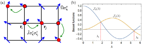
Figure 2: (a) Illustration of the $Z_{2}$ lattice gauge theory given by Hamiltonian (6). Local spins live on each lattice site. Spinless $\hat{c}$-fermions can hope between the lattice sites. The hopping amplitude depends on the configuration of the local spins. (b) Fine tuning of modulations. The solutions of $\mathcal{J}_{0}\left(\lambda\right)=\mathcal{J}_{2}\left(\lambda\right)$ are $\lambda_{1}=1.84118$ and $\lambda_{2}=5.33144$.

The Hamiltonian (6) can also be dualed to the standard $Z_{2}$ lattice gauge theory, where gauge fields $\tau$ are defined on the link, with coupling terms $\hat{c}_{\mathbf{r}+\mathbf{a}_{i}}^{{\dagger}}\hat{c}_{\mathbf{r}}\tau_{\mathbf{r}}^{z}$, star terms $\prod_{+}\tau_{\mathbf{r+a_{i}}/2}^{x}$ and flux terms $\prod_{\square}\tau_{\mathbf{r}}^{z}$ in the Hamiltonian. We could define the duality $\tau_{\mathbf{r+a_{i}}/2}^{z}=\sigma_{\mathbf{r}+\mathbf{a}_{i}}^{z}\sigma_{\mathbf{r}}^{z}$. The the first term in (6) becomes the standard coupling term and the second term becomes the star term. Moreover, the definition imposes that $\prod_{\square}\tau_{\mathbf{r}}^{z}=1$, which is equivalent to having a large flux term.

Symmetry. Unlike the density-dependent gauge fields without local gauge symmetry DDGF@Chin.2018 ; DDGF@Esslinger.2019 ; Cavity_SOC@Lev.2019 , our model possesses a local $Z_{2}$ gauge symmetry at each site. The gauge transformation operator is given by

$$\hat{G}_{\mathbf{r}}=e^{i\pi\hat{n}_{\mathbf{r}}^{c}}\sigma_{\mathbf{r}}^{x}.$$ (7)

It is easy to check $[\hat{G}_{\mathbf{r}},\hat{H}_{\mathrm{eff}}]=0$, and $[\hat{G}_{\mathbf{r}_{2}},\hat{G}_{\mathbf{r}_{1}}]=0$ for any given site. That means the eigenstates of the Hamiltonian is also the eigenstates of $\hat{G}_{\mathbf{r}}$, $\hat{G}_{\mathbf{r}}\left|\psi\left(\mathbf{g}\right)\right\rangle=g_{\mathbf{r}}\left|\psi\left(\mathbf{g}\right)\right\rangle$, where vector $\mathbf{g}=\left(g_{\mathbf{r}_{1}},g_{\mathbf{r}_{2}},\cdots\right)$. Here the eigen value $g_{\mathbf{r}}=\pm 1$. This separates the Hilbert space into different subsectors. In each subsector, $\hat{G}_{\mathbf{r}}$ is a good quantum number, giving $e^{i\pi\hat{n}_{\mathbf{r}}^{c}}g_{\mathbf{r}}=\sigma_{\mathbf{r}}^{x}$, which is nothing but the $Z_{2}$ Gauss’s law similar to the electrodynamics. The $e^{i\pi\hat{n}_{\mathbf{r}}^{c}}$ is the $Z_{2}$ charge carried by matter field, the $g_{\mathbf{r}}$ is the local black ground charge, and $\sigma_{\mathbf{r}}^{x}$ is the electrical field. In real life, we are constrained in one subspace of the $U(1)$ gauge theory, where the background charge is zero. However in our synthetic world, we can prepare the initial states at different subspaces, or even the superposition of several subsectors. That leads richer dynamics of the gauge field.

Making a unitary transformationZ2LGT@Maciejko.2017 , $U=e^{i\frac{\pi}{2}\sum\nolimits_{\mathbf{r}}\sigma_{\mathbf{r}}^{z}\hat{n}_{\mathbf{r}}^{c}}$, we find that the matter field and the gauge field are bound,

$$\hat{c}_{\mathbf{r}} \longrightarrow -i\sigma_{\mathbf{r}}^{z}\hat{c}_{\mathbf{r}},$$ (8)

$$\sigma_{\mathbf{r}}^{z} \longrightarrow \sigma_{\mathbf{r}}^{z},$$ (9)

$$\sigma_{\mathbf{r}}^{x} \longrightarrow \sigma_{\mathbf{r}}^{x}-2\sigma_{\mathbf{r}}^{x}\hat{n}_{\mathbf{r}}.$$ (10)

As a results, the Hamiltonian and $\hat{G}_{\mathbf{r}}$ transforms into

$$\hat{H}^{\prime} = \tilde{J}\sum\limits_{\mathbf{r},i}(\hat{c}_{\mathbf{r}+\mathbf{a}_{i}}^{{\dagger}}\hat{c}_{\mathbf{r}}+h.c.)+\tilde{\Omega}\sum\limits_{\mathbf{r}}\sigma_{\mathbf{r}}^{x}\left(1-2\hat{n}_{\mathbf{r}}\right),$$

$$\hat{G}_{\mathbf{r}}^{\prime} = \sigma_{\mathbf{r}}^{x},$$ (11)

Note that after transformation, Hamiltonian explicitly includes local gauge transformation operator. In one particular subsector, $\hat{G}_{\mathbf{r}}^{\prime}$ is a good quantum number, and can be replaced by its eigen values. So Hamiltonian in this subsector reads

$$\hat{H}_{\mathrm{sub}}\left(\mathbf{g}\right) = \tilde{J}\sum\limits_{\mathbf{r,}i}(\hat{c}_{\mathbf{r}+\mathbf{a}_{i}}^{{\dagger}}\hat{c}_{\mathbf{r}}+h.c.)$$ (12)

$$-2\tilde{\Omega}\sum\limits_{\mathbf{r}}g_{\mathbf{r}}\hat{n}_{\mathbf{r}}^{c}+\tilde{\Omega}\sum\limits_{\mathbf{r}}g_{\mathbf{r}}$$

By constrained in one subsector, this lattice gauge model is mapped into non-interacting fermions moving in the potential of the background charges. These fermions are so-called ”Orthogonal” fermions OF@Sigrist.2010 ; OF@Senthil.2012 ; OF@Sachdev.2019 ; OF@Meng.2020 , which are composite of local spins and $\hat{c}$-fermions. This mapping is similar to the integral out of the longitudinal electrical field to obtain the Coulomb interaction in the Maxwell theory. In our model, there is no Coulomb interaction between the particles, but only the coupling between matter field and the background charges.

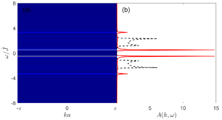
Figure 3: (a) Momentum resolved radio-frequency spectrum function for a half-filled one dimensional lattice at zero-temperature. (b) Radio-frequency spectrum function at a given momentum. The dashed line is the single-particle density-of-state in a spin density wave back ground charge distribution. The calculation is done in a lattice with length $100$, and $\tilde{\Omega}/\tilde{J}=0.6$.

At the half-filling, we numerically found the ground state as $\left|\psi_{\mathrm{gs}}\right\rangle=\hat{U}^{{\dagger}}\left|\varphi_{\mathrm{CDW}}\right\rangle\otimes\left|\mathbf{g}^{\mathrm{SDW}}\right\rangle$ in one dimension. The local spins form a spin density wave (SDW), $g_{\mathbf{r}}^{\mathrm{SDW}}=\left(-1\right)^{\sum\nolimits_{i=1}^{d}r_{i}}$. The ”Orthogonal” fermions form a charge density wave (CDW), $\left|\varphi_{\mathrm{CDW}}\right\rangle$. This ground state can be generalized to two and three dimension. It can be understood in two limits. First if $\tilde{J}\rightarrow 0$, the ground states have $\left\langle\hat{n}_{\mathbf{r}}\right\rangle=1(0)$, as $g_{\mathbf{r}}=+1(-1)$ to lower the on-site energy. There are innumerable states possessing the same energy, but for a finite $\tilde{J}$, the SDW configuration will minimize the kinetic energy at the half-filling. Second, at $\tilde{\Omega}\rightarrow 0$, the ground state is a Fermi sea of the ”Orthogonal” fermions. When openning $\tilde{\Omega}$, the SDW will scattering the ”Orthogonal” fermions by a momentum $\mathbf{Q}=\sum\nolimits_{i=1}^{d}\frac{\pi}{a}\mathbf{e}_{i}$. At the half-filling, it will mach the Fermi surface nesting to open a gap, leading a CDW.

Observations. The first observation is the radio-frequency spectroscopy. Considering the retarder Green’s function of the $\hat{c}$-fermions, $iG_{\mathbf{r}_{2},\mathbf{r}_{1}}^{\mathrm{R}}\left(t\right)=\Theta\left(t\right)\left\langle\{\hat{c}_{\mathbf{r}_{2}}(t),\hat{c}_{\mathbf{r}_{1}}^{{\dagger}}(0)\}\right\rangle$. Transforming into the ”Orthogonal” fermion picture, we have

$$G_{\mathbf{r}_{2},\mathbf{r}_{1}}^{\mathrm{R}}\left(t\right)=\delta_{\mathbf{r}_{2}\mathbf{,r}_{1}}\sum\limits_{\mathbf{g}}S_{\mathbf{r}_{1}}\left(t,\mathbf{g}\right)$$ (13)

Here $iS_{\mathbf{r}}\left(t,\mathbf{g}\right)=\Theta\left(t\right)\sum\limits_{n}\frac{e^{-\beta E_{n}\left(\mathbf{g}\right)}}{Z}\left\langle\varphi_{n}\left(\mathbf{g}\right)\right|\hat{c}_{\mathbf{r}}\times e^{-\frac{i\left[H_{\mathrm{sub}}\left(\mathbf{g}^{\prime}\right)-E_{n}\left(\mathbf{g}\right)\right]t}{\hbar}}\hat{c}_{\mathbf{r}}^{{\dagger}}\left|\varphi_{n}\left(\mathbf{g}\right)\right\rangle+\left(\hat{c}_{\mathbf{r}}\leftrightarrow\hat{c}_{\mathbf{r}}^{{\dagger}},t\leftrightarrow-t\right)$ where $E_{n}\left(\mathbf{g}\right)$ is the eigen energy, $\left|\varphi_{n}\left(\mathbf{g}\right)\right\rangle$ the eigen state of ”Orthogonal” fermion at the given background charge $\mathbf{g}$. The background charge distribution $\mathbf{g}^{\prime}$ is opposite from $\mathbf{g}$ at site $\mathbf{r}$, $\left|\mathbf{g}^{\prime}\right\rangle=\sigma_{\mathbf{r}}^{z}\left|\mathbf{g}\right\rangle$. The prefactor $\delta_{\mathbf{r}_{2}\mathbf{,r}_{1}}$ indicates the single particle(hole) excitations can not propagate, since they are bound with the local spins (8). As a results the momentum resolved radio-frequency spectroscopy, which measured the imaginary part of the retarded Green’s function, shows no dispersion at any given temperature, $A\left(\mathbf{k},\omega\right)=-2\mathrm{Im}G_{\mathbf{0}}^{\mathrm{R}}\left(\omega\right)$. In addition, adding(removing) the $\hat{c}$-fermions to(from) the system, will flip the local spins, which will create an local impurity potential for the ”Orthogonal” fermions, this process is similar to the X-Ray absorption or emission in the solid materials OC@Anderson.1967 ; OC@Mahan.1967 ; OC@Nozieres1 ; OC@Nozieres2 ; OC@Nozieres3 ; OC@Demler.2013 . Using the trace formula OC@Demler.2013 , we calculate the radio-frequency spectrum of a half-filled one dimensional lattice at zero-temperature, see Fig.3. The spectrum exhibits in-gap peaks, which imply bound states of the $\hat{c}$-fermions and local spins.

Second observation is the dynamical localization. Consider the time evolution of the initial states $\left|\psi(0)\right\rangle=\hat{U}^{{\dagger}}\left|\varphi(0)\right\rangle\otimes\prod\limits_{\mathbf{r}}\left|\uparrow\right\rangle_{\mathbf{r}}$, where $\left|\varphi(0)\right\rangle$ is the state of ”Orthogonal” fermions, $\left|\uparrow(\downarrow)\right\rangle_{\mathbf{r}}$ is the local eigenstate of $\sigma_{\mathbf{r}}^{z}$. One can expand $\left|\uparrow\right\rangle_{\mathbf{r}}$ by the local eigenstates of $\hat{G}_{\mathbf{r}}^{\prime}$, $\left|\uparrow\right\rangle_{\mathbf{r}}=\frac{1}{2}\left(\left|+1\right\rangle_{\mathbf{r}}+\left|-1\right\rangle_{\mathbf{r}}\right)$. So the initial state can be rewritten into $\left|\psi(0)\right\rangle=\sqrt{2}^{-N_{\mathrm{s}}}\hat{U}^{{\dagger}}\left|\varphi(0)\right\rangle\otimes\sum_{\mathbf{g}}\left|\mathbf{g}\right\rangle$, where $N_{\mathrm{s}}$ is the number of lattice site. Note that this wave function is a superposition of different subspaces. If we focus on the behavior of the fermions, the expectation value of a fermion operator reads

$$\left\langle O\left(t\right)\right\rangle=\frac{1}{2^{N_{\mathrm{s}}}}\sum_{\mathbf{g}}\left\langle\varphi(0)\right|e^{\frac{iH_{\mathrm{sub}}\left(\mathbf{g}\right)t}{\hbar}}Oe^{-\frac{iH_{\mathrm{sub}}\left(\mathbf{g}\right)t}{\hbar}}\left|\varphi(0)\right\rangle.$$ (14)

We can see that $e^{-\frac{iH_{\mathrm{sub}}\left(\mathbf{g}\right)t}{\hbar}}\left|\varphi(0)\right\rangle$ is the time evolution of the non-interacting ”Orthogonal” fermions in a subsector with given background charge distribution. The summation is identical to the ensemble average of the ”Orthogonal” fermions moving in disorder potential. So this dynamics is similar to the Anderson model, expect the potential here is binary distribution rather than the uniform distribution. In one or two dimension this dynamics exhibits the localization Localization@Moessner.2017 ; Localization@Scardicchio.2018 ; Localization@Kovrizhin.2018 ; Localization@Langari.2019 ; Localization@Zhai.2020 ; Localization@Knolle.2020 . However start with the initial state $\hat{U}^{{\dagger}}\left|\varphi(0)\right\rangle\otimes\prod_{\mathbf{r}}\left|+1\right\rangle_{\mathbf{r}}$, which is in one subsector. The ”Orthogonal” fermions feel a uniform potential, no background charge fluctuations. There will be no localization. We calculate the spreading of a single fermion wavepacket in one dimension, see Fig.4. Starting from the uniform background charges, the width of the wavepacket, $W=\sqrt{\left\langle\sum\nolimits_{\mathbf{r}}\mathbf{r}^{2}\hat{c}_{\mathbf{r}}^{{\dagger}}\hat{c}_{\mathbf{r}}\right\rangle-\left\langle\sum\nolimits_{\mathbf{r}}\mathbf{r}\hat{c}_{\mathbf{r}}^{{\dagger}}\hat{c}_{\mathbf{r}}\right\rangle^{2}}$, grows linear with the time. However if the initial state is a superposition state, the width is saturated at long time. So the disorder effect in the dynamics is led by the background charge fluctuation, which is the consequence of the superposition initial states.

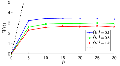
Figure 4: Wavepacket spreading of one fermion in one dimension lattice gauge field. The initial state of the solid lines is $\hat{U}^{{\dagger}}\hat{c}_{\mathbf{0}}^{{\dagger}}\left|0\right\rangle\otimes\prod_{\mathbf{r}}\left|\uparrow\right\rangle_{\mathbf{r}}$, while the initial state of the dashed line is $U^{{\dagger}}\hat{c}_{\mathbf{0}}^{{\dagger}}\left|0\right\rangle\otimes\prod_{\mathbf{r}}\left|+1\right\rangle_{\mathbf{r}}$. The simulation is done on a lattice with length $21$.

Summary. We propose a Floquet approach to simulate a simple lattice gauge model. Our method is feasible with current experiment techniques, and can be implemented in extend system in one, two or three dimensions. The effective Hamiltonian is obtained by keeping to the zeroth order of $1/\omega$ expansion. The next order processes with break the local gauge symmetry. However, those terms are high suppressed in the large driving frequency limit, such that the gauge invariant dynamics will not be affected in the typical time scale of the experiment.

References

(1) J. B. Kogut, Rev. Mod. Phys. 51, 659
(1979).
(2) L. Balents, Nature 464, 199 (2010).
(3) N. Read, and S. Sachdev, Phys. Rev. Lett.
66, 1773 (1991).
(4) R. A. Jalabert, S. Sachdev, Phys. Rev. B
44, 686 (1991).
(5) G. Baskaran and P. W. Anderson, Phys. Rev. B
37, 580 (1988).
(6) N. Read and S. Sachdev, Phys. Rev. B 42,
4568 (1990).
(7) I. Affleck and J. B. Marston, Phys. Rev. B 37, 3774 (1988).
(8) T. Senthil, M. P. A. Fisher, Phys. Rev. B 62, 7850 (2000).
(9) S. A. Kivelson, D. S. Rokhsar, and J. P. Sethna,
Phys. Rev. B 35, 8865 (1987).
(10) R. Moessner, S. L. Sondhi, and E. Fradkin, Phys.
Rev. B 65, 024504 (2001).
(11) E. A. Martinez, C. A. Muschik, P. Schindler, D.
Nigg, A. Erhard, M. Heyl, P.p Hauke, M. Dalmonte, T. Monz, P. Zoller, and R.
Blatt, Nature 534, 516 (2016).
(12) C. Schweizer, F. Grusdt, M. Berngruber, L.
Barbiero, E. Demler, N. Goldman, I. Bloch, M. Aidelsburger, Nat. Phys.
15, 1168 (2019)
(13) B. Yang, H. Sun, R. Ott, H.-Y. Wang, T. V. Zache,
J. C. Halimeh, Z.-S. Yuan, P. Hauke, J.-W. Pan, arXiv:2003.08945v2
(14) A. Mil, T. V. Zache, A. Hegde, A. Xia, R.
P. Bhatt, M. K. Oberthaler, P. Hauke,J. Berges, and F. Jendrzejewski,
Science 367, 1128 (2020)
(15) L. W. Clark, B. M. Anderson, L. Feng, A. Gaj, K.
Levin, and C. Chin, Phys. Rev. Lett. 121, 030402 (2018).
(16) F. Görg, K. Sandholzer, J. Minguzzi, R.
Desbuquois, M. Messer, and T. Esslinger, Nat. Phys. 15, 1161 (2019).
(17) R. M. Kroeze, Y. Guo, and B. L. Lev,
arXiv:1904.08388
(18) U. Wiese, Ann. Phys. (Berlin) 525, 777
(2013).
(19) L. Barbiero, C. Schweizer, M. Aidelsburger, E.
Demler, N. Goldman, Fa. Grusdt, Sci. Adv. 5, 7444 (2019)
(20) F. F. Assaad and Tarun Grover, Phys. Rev. X
6, 041049 (2016).
(21) E. Zohar, A. Farace, B. Reznik, and J. I. Cirac,
Phys. Rev. Lett. 118, 070501 (2017)
(22) Y.-J. Lin, R. L. Compton, K. Jiménez-García, W. D. Phillips,
J. V. Porto, and I. B. Spielman, Nat. Phys. 7, 531 (2011)
(23) Y.-J. Lin, R. L. Compton, K. Jiménez-García, J. V. Porto, and I. B. Spielman,
Nature 46, 628 (2009)
(24) Y.-J. Lin, K. Jiménez-García, and I. B. Spielman, Nature 471, 83 (2011)
(25) Z. Wu, L. Zhang, W. Sun, X.-T. Xu, B.-Z. Wang, S.-C. Ji, Y. Deng, S. Chen, X.-J. Liu, J.-W. Pan,
Science 354, 83 (2016)
(26) M. Aidelsburger, S. Nascimbene, N. Goldman, C. R. Physique 19, 394 (2018)
(27) A. Rüegg, S. D. Huber and M. Sigrist, Phys.
Rev. B 81, 155118 (2010)
(28) R. Nandkishore, M. A. Metlitski and T. Senthil,
Phys. Rev. B 86, 045128 (2012)
(29) S. Gazit, F. F. Assaad and S. Sachdev,
arXiv:1906.11250
(30) C. Chen, X. Y. Xu, Y. Qi, Z. Y. Meng, Chin. Phys.
Lett. 37, 047103 (2020)
(31) C. Prosko, S.-P. Lee, and J. Maciejko, Phys.
Rev. B 96, 205104 (2017).
(32) P. W. Anderson, Phys. Rev. 164, 352
(1967).
(33) G. D. Mahan, Phys. Rev. 153, 882 (1967).
(34) B. Roulet, J. Gavoret, and P. Nozières, Phys.
Rev. 178, 1072 (1969).
(35) P. Nozières, B. Roulet, and J. Gavoret, Phys.
Rev. 178, 1084 (1969).
(36) P. Nozières, and C. T. De Dominicis, Phys. Rev.
178, 1097 (1969).
(37) D. Benjamin, D. Abanin, P. Abbamonte, and E.
Demler, Phys. Rev. Lett. 110, 137002 (2013).
(38) A. Smith, J. Knolle, D. L. Kovrizhin,
and R. Moessner, Phys. Rev. Lett. 118, 266601 (2017).
(39) M. Brenes, M. Dalmonte, M. Heyl, and
A. Scardicchio, Phys. Rev. Lett. 120, 030601 (2018)
(40) A. Smith, J. Knolle, R. Moessner, and
D. L. Kovrizhin, Phys. Rev. B 97, 245137 (2018)
(41) H. Yarloo, M. Mohseni-Rajaee, and A.
Langari, Phys. Rev. B 99, 054403 (2019)
(42) Z. Yao, C. Liu, P. Zhang, H. Zhai, Phys.
Rev. B 102, 104302 (2020)
(43) I. Papaefstathiou, A. Smith, and J.
Knolle, arXiv:2003.12497v1