Study of the axial $U(1)$ anomaly at high temperature with lattice chiral fermions

Abstract

We investigate the axial $U(1)$ anomaly of two-flavor QCD at temperatures 190–330 MeV. In order to preserve precise chiral symmetry on the lattice, we employ the Möbius domain-wall fermion action as well as overlap fermion action implemented with a stochastic reweighting technique. Compared to our previous studies, we reduce the lattice spacing to 0.07 fm, simulate larger multiple volumes to estimate finite size effect, and take more than four quark mass points, including one below physical point to investigate the chiral limit. We measure the topological susceptibility, axial $U(1)$ susceptibility, and examine the degeneracy of $U(1)$ partners in meson/baryon correlators. All the data above the critical temperature indicate that the axial $U(1)$ violation is consistent with zero within statistical errors. The quark mass dependence suggests disappearance of the $U(1)$ anomaly at a rate comparable to that of the $SU(2)_{L}\times SU(2)_{R}$ symmetry breaking.

I Introduction

The two-flavor QCD Lagrangian in the massless limit has a global $SU(2)_{L}\times SU(2)_{R}\times U(1)_{V}\times U(1)_{A}$ symmetry. It is widely believed that its $SU(2)_{L}\times SU(2)_{R}$ part is spontaneously broken to $SU(2)_{V}$ at low temperatures but is restored above some critical temperature, which is called the chiral phase transition. On the other hand, the axial $U(1)_{A}$ part is broken by the chiral anomaly. Since the anomaly refers to symmetry breaking at the cut-off scale where the theory is defined, and the anomalous Ward-Takahashi identity holds at any temperature Itoyama:1982up , it is natural to assume that the anomaly survives the chiral phase transition and the physics of the early universe is not $U(1)_{A}$ symmetric.

However, there is a counter argument to this naive picture. In fact, the $U(1)_{A}$ anomaly is connected to the topology of the gauge field, which is sensitive to the low energy dynamics, and low-lying modes of the Dirac operator affect the strength of the $U(1)_{A}$ violation. In particular, if the Dirac spectrum has a gap at the lowest end of the spectrum, the $U(1)_{A}$ anomaly becomes invisible in two-point mesonic correlation functions in the chiral limit Cohen:1996ng ; Cohen:1997hz . Since the $SU(2)_{L}\times SU(2)_{R}$ symmetry is also related to the Dirac spectrum through the Banks-Casher relation Banks:1979yr , the restoration of $SU(2)_{L}\times SU(2)_{R}$ at the chiral transition may also affect the $U(1)_{A}$ anomaly. Indeed, it was argued that the $U(1)_{A}$ anomaly can completely disappear in correlation functions of scalar and pseudoscalar operators Aoki:2012yj .

If the effect of the $U(1)_{A}$ anomaly is negligible at and above the critical temperature, it may have an impact on our understanding of the phase diagram of QCD Pisarski:1983ms . In the standard effective theory analysis of the chiral phase transition, we expect only the pion and its chiral-partner scalar particle to be the light degrees of freedom that govern the low-energy dynamics of QCD near the phase transition. When the $U(1)_{A}$ symmetry is effectively restored, the $\eta$, isospin singlet pseudoscalar, and its chiral partner may play a nontrivial role Horvatic:2018ztu ; Bass:2018xmz ; Nicola:2019ohb . Since the effective potential can have more complicated structure as the degrees of freedom increase, it was argued that the chiral phase transition likely becomes first order when $U(1)_{A}$ symmetry is recovered (we refer the readers to Yonekura:2019vyz for a different aspect of the first-order scenario from ’t Hooft anomaly matching), though other scenarios are theoretically possible Pelissetto:2013hqa ; Nakayama:2014sba ; Kanazawa:2014cua ; Sato:2014axa ; Nakayama:2016jhq ; Alexandru:2019gdm .

How much the $U(1)_{A}$ anomaly contributes to the dynamics has a significant importance on cosmology. The topological susceptibility is related to the mass and decay constant of the QCD axion, which is a candidate of the dark matter. Its temperature dependence influences the relic abundance of the axion Berkowitz:2015aua ; Kitano:2015fla ; Bonati:2015vqz ; Petreczky:2016vrs ; Borsanyi:2016ksw ; Burger:2018fvb ; Lombardo:2020bvn .

For the nontrivial question of how much the $U(1)_{A}$ anomaly remains and affects the chiral phase transition, only lattice QCD can give a quantitative answer. Good control of chiral symmetry on the lattice Bazavov:2012qja ; Cossu:2013uua ; Buchoff:2013nra ; Chiu:2013wwa is necessary in order to precisely discriminate between the lattice artifact and the physical signal that survives in the continuum limit. Our previous studies Cossu:2015kfa ; Cossu:2016scb ; Tomiya:2016jwr demonstrated that the signal of topological susceptibility is sensitive to the violation of chiral symmetry at high temperature, and the reweighting of the Möbius domain-wall fermion determinant to that of the overlap fermion is essential when the lattice spacing is coarse $a\gtrsim 0.1$ fm. We also found that the use of the overlap fermion only in the valence sector Dick:2015twa ; Sharma:2018syt ; Mazur:2018pjw makes the situation worse, since the lattice artifact due to the mixed action, which is unphysical, is strongly enhanced.

After removing the lattice artifact due to the violation of the Ginsparg-Wilson relation at high temperature, we observed that chiral limit of the $U(1)_{A}$ susceptibility is consistent with zero Tomiya:2016jwr . The disappearance of the $U(1)_{A}$ anomaly (at around 1.2 $T_{c}$) was also reported by other groups simulating non-chiral fermions Brandt:2016daq ; Ishikawa:2017nwl . In Bazavov:2019www , it was found that the $U(1)_{A}$ symmetry shows up at 1.3 $T_{c}$ but not around $T_{c}$ .

In this work, we reinforce the conclusion of Tomiya:2016jwr by 1) reducing the lattice spacing to an extent where we observe consistency between the overlap and Möbius domain-wall fermions, 2) simulating different lattice volume sizes in a range $1.8\leq L\leq 3.6$ fm, and 3) simulating more quark mass points, including one below the physical point, to investigate the chiral limit. In order to study possible artifact due to topology freezing, we also apply the reweighting from a larger quark mass, where topology tunneling is frequent, down to the mass where the topological susceptibility is consistent with zero. We measure the topological susceptibility, axial $U(1)$ susceptibility, meson correlators, and baryon correlators. Some of the results were already reported in our contributions to the conference proceedings Aoki:2017xux ; Suzuki:2017ifu ; Fukaya:2017wfq ; Suzuki:2018vbe ; Suzuki:2019vzy ; Rohrhofer:2019yko ; Suzuki:2020rla .

All the data at temperatures above 190 MeV show that the axial $U(1)$ anomaly is consistent with zero, within statistical errors. Its quark mass dependence indicates that the disappearance of the $U(1)$ anomaly is at a rate comparable to that of the $SU(2)_{L}\times SU(2)_{R}$ symmetry. At higher temperature, we have also observed a further enhancement of symmetry Rohrhofer:2017grg ; Glozman:2017dfd ; Lang:2018vuu ; Rohrhofer:2019qwq .

The rest of the paper is organized as follows. We describe our lattice setup and how to implement the chiral fermions in the simulations in Sec. II. In Sec. III, the numerical results for the Dirac spectrum, topological susceptibility, axial $U(1)$ susceptibility, and meson/baryon screening masses are presented. The conclusion is given in Sec. IV.

II Lattice setup

The setup of our simulations is basically the same as our previous study Tomiya:2016jwr , except for the choice of parameters (larger lattice sizes up to $3.6$ fm, and smaller lattice spacing $a\sim 0.074$ fm). Our naive estimate for the critical temperature of the chiral phase transition in Tomiya:2016jwr is $T_{c}\sim 175$ MeV, which was obtained from the Polyakov loop. Below, we summarize the essential part.

In the hybrid-Monte-Carlo (HMC) simulations, we employ the tree-level improved Symanzik gauge action Luscher:1985zq for the link variables and the domain-wall fermion Kaplan:1992bt with an improvement (the Möbius domain-wall fermions Brower:2005qw ; Brower:2012vk ) for the quark fields. Here we set the size of the fifth direction as $L_{s}=16$. The Möbius kernel is taken as

$$H_{M}=\gamma_{5}\frac{2D_{W}}{2+D_{W}},$$ (1)

where $D_{W}$ is the standard Wilson-Dirac operator with a large negative mass $-1/a$. In the following, we omit $a$, when there is no risk of confusion. The numbers without physical unit, e.g. MeV, are in the lattice unit. The fermion determinant thus obtained corresponds to a four-dimensional effective operator,

$$D_{\rm DW}^{\rm 4D}(m)=\frac{1+m}{2}+\frac{1-m}{2}\gamma_{5}\tanh(L_{s}\tanh^{-1}(H_{M})).$$ (2)

Note that if we take the $L_{s}=\infty$ limit, this operator converges to the overlap-Dirac operator Neuberger:1997fp with a kernel operator $H_{M}$. The stout smearing Morningstar:2003gk is applied three times with the smoothing parameter $\rho=0.1$ for the link variables in the Dirac operator.

The residual mass for our main runs at $\beta=4.30$ is 0.14(6) MeV, which may look small enough for the measurements in this work. However, as we reported in our previous studies, the chiral symmetry breaking due to lattice artifacts is enhanced at high temperature, in particular for the axial $U(1)$ susceptibility. Therefore, we employ an improved Dirac operator, exactly treating the near-zero modes of $H_{M}$ to compute the sign function. With the near-zero modes whose absolute value is less than 0.24 ($\sim 630$ MeV) treated exactly, we find that the residual mass becomes negligible $\sim 10^{-5}$ or $\sim$ 0.01 MeV. Although it is different from the original definition in Neuberger:1997fp , we call this improved Dirac operator the “overlap” Dirac operator $D_{ov}(m)$. Note that our overlap operator has a finite $L_{s}$, i.e. $L_{s}=16$. As we also found in our previous study that the lattice artifact from mixed action is large even though the overlap and Möbius domain-wall fermion actions are very similar to each other, we reweight the gauge configurations of the Möbius domain-wall fermion determinant by that of the overlap fermion. For details of this OV/MDW reweighting, see Tomiya:2016jwr . As we will see below, at $\beta=4.30$ the results with the overlap fermion and those with Möbius domain-wall fermion are consistent with each other, except for the $U(1)$ susceptibility at $T\leq 260$ MeV. For the meson and baryon correlators, we use the Möbius domain-wall fermion without reweighting.

The lattice spacing is estimated from the Wilson flow with a reference flow time $t_{0}=(0.1539\;\mbox{fm})^{2}$ determined in Sommer:2014mea . For our main runs at $\beta=4.30$, the physical point of the bare quark mass is estimated as $m=0.0014(2)$, which is slightly above our lightest quark mass. For this estimate, we used a leading-order chiral perturbation formula, with an input of simulated pion mass $m_{\pi}=0.135(8)$ (in the lattice units) determined from a zero temperature study at $m=0.01$. The choice of the simulation parameters enables us to interpolate the results to the physical point.

The simulation parameters are summarized in Tab. 1. Compared to the previous work Tomiya:2016jwr , we reduce the lattice spacing from $\sim 0.1$ fm to 0.074 fm. At this value of lattice spacing, we change temperatures by varying the temporal extent $L_{t}=8,10,12,14$, which correspond to temperatures $T=$ 190–330 MeV. In order to estimate the finite volume effects, we simulate with four different volume sizes $L^{3}$ with $L=24,32,40$ and 48 at $T=220$ MeV. We also increase the statistics at $\beta=4.24$ ensembles continued from Tomiya:2016jwr to check the consistency between different lattice spacings.

For each ensemble, we simulated more than 20000 trajectories from which we carry out measurements on the configurations separated by 100 trajectories. We then bin the data in every 1000 trajectories, which is longer than autocorrelation lengths we observe. When we use the OV/MDW reweighting, we lose some amount of statistics due to its noise. An estimate for the effective number of statistics $N_{\rm rew}$ in the table is defined as

$$N_{\rm rew}=\frac{\langle R\rangle}{R_{\rm max}},$$ (3)

where $R$ is the reweighting factor or the ratio of the determinant and $R_{\rm max}$ is its maximal value in the ensemble. As discussed in Tomiya:2016jwr , $R$ has a negative correlation with the axial $U(1)$ observables, and the statistical error estimated by the jackknife method are smaller than expected from $1/\sqrt{N_{\rm rew}}$. For the ensembles with small number of $N_{\rm rew}\sim 10$, it is important to check the consistency with the Möbius domain-wall results without reweighting.

$\beta$	$a$(fm)	$L^{3}\times L_{t}$	$T$(MeV)	$L$(fm)	$m$	#trj.	$N_{\rm rew}$	comments
4.24	0.084	$32^{3}\times 12$	195	2.7	0.0025	21200	10(2)
					0.005	20000	10(1)	continuation from Tomiya:2016jwr
					0.01	25300	7(1)
4.30	0.074	$32^{3}\times 14$	190	2.4	0.001	13900	38(2)
					0.0025	16600	8(1)
					0.00375	12500	10(1)
					0.005	10600	9(1)
		$24^{3}\times 12$	220	1.8	0.001	31900	50(1)
					0.0025	33400	49(1)
					0.00375	34600	17(1)
					0.005	36000	16(1)
					0.01	35900	47(2)
		$32^{3}\times 12$	220	2.4	0.001	26500	32(1)
					0.0025	26660	57(2)
					0.00375	26420	28(2)
					0.005	18560	30(1)
					0.01	31000	93(2)
		$40^{3}\times 12$	220	3.0	0.005	28100	13(1)
					0.01	27300	39(2)
		$48^{3}\times 12$	220	3.6	0.001	11200	4(1)
					0.0025	11300	8(1)
					0.00375	12800	10(2)
					0.005	10900	2(1)
		$32^{3}\times 10$	260	2.4	0.005	12780	25(1)	$m_{r}=0.003,0.004$
					0.008	20050	19(1)
					0.01	29000	58(2)	$m_{r}=0.006,0.007,0.008,0.009$
					0.015	12000	20(1)
		$32^{3}\times 8$	330	2.4	0.001	26100	42(2)
					0.005	31700	28(2)
					0.01	24500	37(5)
					0.015	30500	61(2)
					0.02	19100	39(2)	$m_{r}=0.0125,0.015,0.0175$
					0.04	5000	12(1)
		$48^{3}\times 8$	330	3.6	0.01	9000	19(2)
					0.015	13950	17(2)

Table 1: Simulation parameters. The values of $m_{r}$ are taken for the mass reweighting on that particular ensemble. $N_{\rm rew}$ denotes the effective number of configurations after the OV/MDW reweighting (see the main text). The $\beta=4.24$ runs are continuation from Tomiya:2016jwr to check the consistency.

III Numerical results

In this section, we show our numerical results on the axial $U(1)$ anomaly. For meson and baryon correlators, we also present the tests of the $SU(2)_{L}\times SU(2)_{R}$ symmetry for comparison.

III.1 Dirac spectrum

The spectral density of the Dirac operator

$$\rho(\lambda)=\frac{1}{V}\sum_{i}\langle\delta(\lambda-\lambda_{i})\rangle,$$ (4)

in volume $V$ is used as a probe of chiral symmetry breaking. Here, $\lambda_{i}$ denotes the $i$-th eigenvalue of the Dirac operator on a given gauge configuration and $\langle\cdots\rangle$ is the gauge ensemble average. In the chiral limit after taking the thermodynamical limit, we obtain the Banks-Casher relation Banks:1979yr , which relates the chiral condensate $\langle\bar{q}q\rangle$ to the spectrum at $\lambda=0$:

$$\langle\bar{q}q\rangle=\pi\rho(0).$$ (5)

We expect that $\rho(0)=0$ above the critical temperature of the chiral phase transition.

As the vacuum expectation value (vev) $\langle\bar{q}q\rangle$ also breaks the axial $U(1)$ symmetry, the details of $\rho(\lambda)$ in the vicinity of zero is important in this work. It has been shown that if the spectrum has a finite gap at $\lambda=0$, the anomaly becomes invisible in mesonic two-point functions Cohen:1996ng ; Cohen:1997hz . In Ref. Aoki:2012yj , it is argued that the $SU(2)_{L}\times SU(2)_{R}$ symmetry restoration requires $\rho(\lambda)\sim\lambda^{\alpha}$ with the power $\alpha>2$, which is sufficient to show the absence of the axial $U(1)_{A}$ anomaly in multi-point correlation functions of scalar and pseudoscalar operators.

We measure the eigenvalues/eigenfunctions of the Hermitian four-dimensional effective Dirac operator $H_{DW}(m)=\gamma_{5}D_{\rm DW}^{\rm 4D}(m)$ and those of the corresponding overlap-Dirac operator. Each eigenvalue $\lambda_{m}$ is converted to the one of massless Dirac operator by $\lambda=\sqrt{\lambda_{m}^{2}-m^{2}}/\sqrt{1-m^{2}}$. Forty lowest (in their absolute value) modes are stored for gauge configurations separated by 100 trajectories. They cover a range from zero to 300–500 MeV.

In Fig. 1, we present the Dirac eigenvalue density of the overlap-Dirac operator at $T=220$ MeV at $L=32$. Here the OV/MDW reweighting is applied. Compared to the solid line which represents the chiral condensate at $T=0$ Cossu:2016eqs , the low-modes are suppressed by an order of magnitude. We observe a sharp peak near zero, which rapidly disappears as quark mass decreases, as expected from the $SU(2)_{L}\times SU(2)_{R}$ symmetry restoration. Since we find no clear gap, a region of $\lambda$ where $\rho(\lambda)=0$, we are not able to conclude if the axial $U(1)$ symmetry is recovered or not from this observable only.

We also compare these results with the Dirac spectral density of the Möbius domain-wall fermion (dashed symbols) in Fig. 1. The agreement is remarkable. On the other hand, when we switch off the OV/MDW reweighting, which we call the non-reweighted overlap fermion setup, we observe a remarkable peak at the lowest bin, as presented in Fig. 2. Similar peaks were reported in Dick:2015twa ; Sharma:2018syt ; Mazur:2018pjw , with overlap fermion only in the valence sector. Our data clearly show that these peaks are due to the lattice artifact of the mixed action.

In order to grasp possible systematic effects due to the finite lattice size, we compare the accumulated histogram

$$A(\lambda)=\int^{\lambda}_{0}d\lambda^{\prime}\rho(\lambda^{\prime})$$ (6)

at three different volumes, $L=24$ (1.8 fm), 32 (2.4 fm), 40 (3.0 fm) in Fig. 3. Except for $L=24$ at $m=0.01$, whose aspect ratio $LT$ is $2$, which is smallest among the data sets, no clear volume dependence is seen. The point $m=0.01$ is the heaviest mass in our simulation set, which is expected to be least sensitive to the volume, but the Dirac low-mode density is rather high, and some remnants of spontaneous $SU(2)_{L}\times SU(2)_{R}$ breaking and associated pseudo Nambu-Goldstone bosons may be responsible for this volume dependence.

We summarize the results at different temperatures in Fig. 4. The higher the temperature, the stronger the suppression of the low modes is. We find a good consistency between the Möbius domain-wall and reweighted overlap results. We also find that $\beta=4.30$ and $4.24$ results are consistent. The quark mass dependence is not very strong except for the lowest bin near $\lambda=0$.

Finally, the quark mass dependence of the eigenvalue density of the reweighted overlap operator near $\lambda=0$ (with the bin size $\sim$ 10 MeV) is presented in Fig. 5. Here both the chiral zero modes and non-chiral pair of near zero-modes are included. It is remarkable that the density of near-zero modes at different temperatures show a steep decrease towards the massless limit and becomes consistent with zero already at finite quark masses. As will be shown below, this behavior of near zero modes is strongly correlated with the signals of the axial $U(1)$ anomaly.

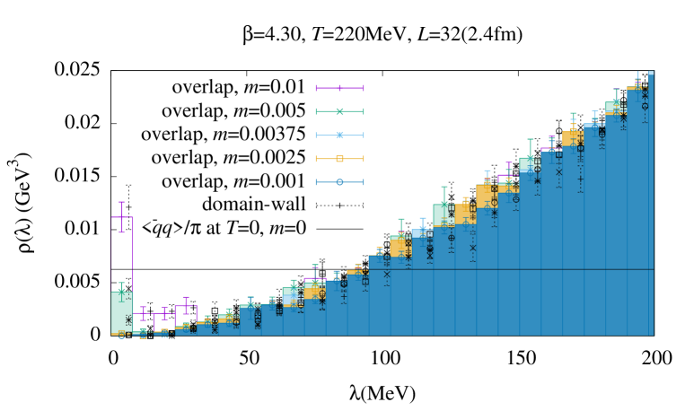
Figure 1: Dirac eigenvalue density at $T=220$ MeV. Solid symbols are the reweighted overlap results and dashed symbols are those of the Möbius domain-wall. Horizontal line shows the chiral limit at $T=0$ Cossu:2016eqs .

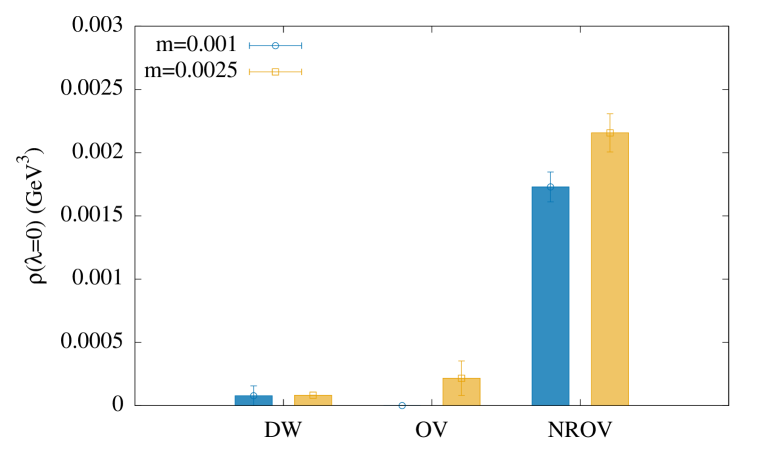
Figure 2: Comparison among Möbius domain-wall (MDW), reweighted overlap (OV), and non-reweighted overlap (NROV) data at the lowest bin with a bin size $\sim$ 10 MeV. A striking enhancement is seen for NROV, which is due to the lattice artifact in the mismatch of the valence and sea actions.

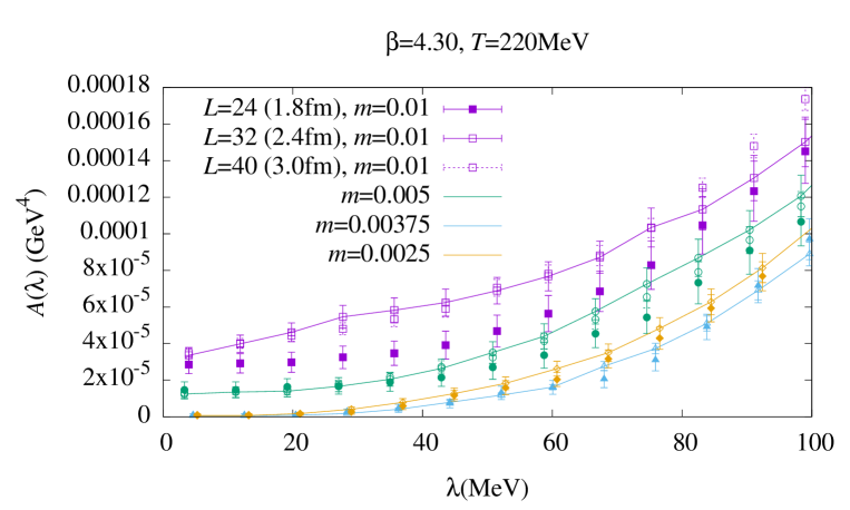
Figure 3: Accumulated Dirac histogram at three different volumes. Data at $m=0.01$ (square symbols), $0.005$ (circles), $0.00375$ (triangles) and $0.0025$ (diamonds) with $L=24$ (filled), $L=32$ (open with solid line) and $L=40$ (open dashed) are shown. Except for $m=0.01$ (squares), the data at different volume sizes are consistent.

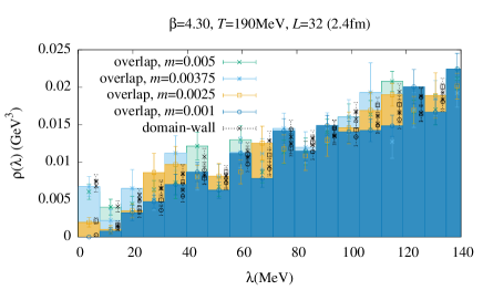
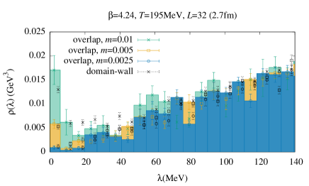
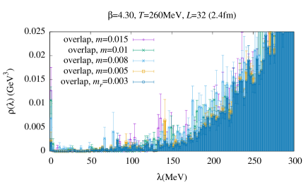
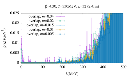
Figure 4: Dirac eigenvalue density at different temperatures.

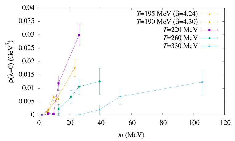
Figure 5: Quark mass dependence of the Dirac eigenvalue density at (near) zero with the bin size $\sim 10$ MeV. All the data look consistent with zero before reaching the chiral limit.

III.2 Topological susceptibility

In order to quantify the topological excitations of gauge fields, we measure the topological charge $Q$ in two different ways. One is the index of the overlap-Dirac operator, or the number of zero modes with positive chirality minus that with negative chirality. For this, we perform the OV/MDW reweighting to avoid possible mixed action artifacts, which is found to be quite significant. The other is a gluonic definition, measured directly on the Möbius domain-wall ensemble, using the clover-like construction of the gauge field strength $F_{\mu\nu}$ after applying the Wilson flow on the gauge configuration with a flow time $ta^{2}=5$.

The results for the topological susceptibility $\chi_{t}=\langle Q^{2}\rangle/V$ obtained at $T=220$ MeV are shown in Fig. 6. The filled symbols show the data for the index of the overlap-Dirac operator with the OV/MDW reweighting, while the dotted symbols are those for gluonic definition without reweighting. Both are consistent with each other. The systematics due to chiral symmetry violating lattice artifacts is therefore under control. We also find that there is no strong volume dependence, except for the heaviest point with $L=1.8$ fm where the aspect ratio is $LT=2$.

In Fig. 8, we present the data at various temperatures. The volume size is fixed to $L=32$ (2.4 fm), except for data at $T=195$ MeV ($\beta=4.24$) (2.7 fm) denoted by diamonds and those at $T=330$ MeV (3.6 fm) by crosses. Here the filled symbols are those obtained with reweighting from the ensemble at a higher mass point shown by open symbols. Even on the configurations where topology fluctuates frequently, the reweighted results decrease towards the chiral limit, which is consistent with the non-reweighted data. See Tab. 1 for the ensembles and masses to which we applied the mass reweighting.

In order to focus on the region near the chiral limit and compare the scale of $\chi_{t}$ compared to the temperature, we plot the same data in Fig. 8 taking the fourth root of $\chi_{t}$ and normalizing it by $T$. It suggests that the topological susceptibility near the chiral limit is suppressed to the level of $O(10)$ MeV with a power $\sim m^{4}$ (or $\chi_{t}^{1/4}\sim m$). The results are not precise enough to determine if $\chi_{t}$ goes to zero at finite quark mass, as predicted in Aoki:2012yj .

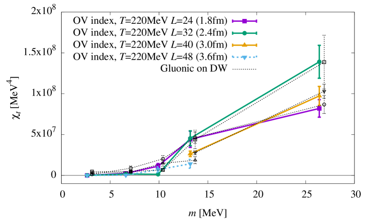
Figure 6: Topological susceptibility at $T=220$ MeV. The filled symbols with solid lines show the data for the index of the overlap-Dirac operator with the OV/MDW reweighting. Those with dashed lines are data at $L=48$ whose statistics may not be good enough after the reweighting. The dotted symbols are those for gluonic definition directly measured on the ensembles generated with the Möbius domain-wall fermions. We confirm that both data with different volumes are consistent.

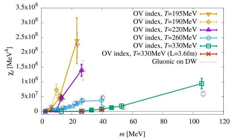
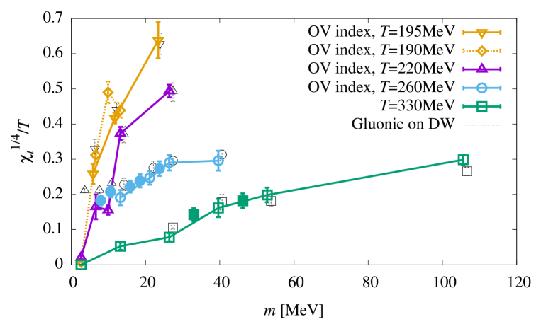
Figure 7: Topological susceptibility at different temperatures. The volume size is fixed to $L=32$ (2.4 fm), except for data at $T=195$ MeV ($\beta=4.24$) (2.7 fm) and those at $T=330$ MeV (3.6 fm) denoted by cross symbols. Filled symbols are obtained with reweighting from the ensemble at a higher mass point shown by open symbols.

Figure 8: The same as Fig. 8 but the fourth root is taken and normalized by $T$. The data suggest that the topological susceptibility near the chiral limit is suppressed to the level of $<10$ MeV as $\chi_{t}^{1/4}/T\sim m$.

III.3 Axial $U(1)$ susceptibility

Let us investigate a more direct measure of the violation of the axial $U(1)$ symmetry, i.e. the axial $U(1)$ susceptibility, defined by the difference between the pseudoscalar ($\pi$) and scalar ($\delta$) correlators integrated over spacetime,

$$\Delta(m)=\sum_{x}\left[\langle\pi(x)\pi(0)\rangle-\langle\delta(x)\delta(0)\rangle\right],$$ (7)

where the ensemble average is taken at a finite quark mass $m$. For the overlap-Dirac operator, we can express $\Delta(m)$ using the spectral decomposition (see Cossu:2015kfa for the details):

$$\Delta(m)=\frac{1}{V(1-m^{2})^{2}}\left\langle\sum_{\lambda_{m}}\frac{2m^{2}(1-\lambda_{m}^{2})^{2}}{\lambda_{m}^{4}}\right\rangle,$$ (8)

where $\lambda_{m}$’s are the eigenvalues of $H_{ov}(m)\equiv\gamma_{5}D_{ov}(m)$. Although this equality holds even in a finite volume, we must take the thermodynamical limit before taking the chiral limit.

In our previous study Tomiya:2016jwr , we found that the contribution from chiral zero modes is quite noisy. As an alternative, we subtract the zero-mode contribution, for which $\lambda_{m}=m$, and define

$$\bar{\Delta}(m)\equiv\Delta(m)-\frac{2\langle|Q|\rangle}{m^{2}(1-m^{2})^{2}V},$$ (9)

where $Q$ is the index of the overlap-Dirac operator. We remind the reader that the index $Q$ is equal to the topological charge of the gauge field. This subtraction is justified because in the thermodynamical limit, while at a fixed temperature, $\langle|Q|\rangle$ scales as $V^{1/2}$ ($=L^{3/2}$), and thus the zero-mode contributions vanish in the large volume limit as $1/V^{1/2}$. We numerically confirm this scaling at $T=220$ MeV as presented in Fig. 9. The $L^{3/2}$ scaling of $\langle|Q|\rangle$ looks saturated for $1/(TL)<0.4$. Therefore, $\bar{\Delta}(m)$ in the thermodynamical limit coincides with $\Delta(m)$.

In this work, we further refine the observable by removing the UV divergence. From a simple dimensional analysis of the spectral expression in Eq. (8), the valence quark mass $m_{v}$ dependence of $\bar{\Delta}(m)$ can be expanded as

$$\frac{A}{m_{v}^{2}}+B+m_{v}^{2}C+O(m_{v}^{4}),$$ (10)

and $C$ has a logarithmic UV divergence. What we are interested in is the divergence free piece $\frac{A}{m_{v}^{2}}+B$ and if it is zero or not in the chiral limit. Note that $A$ and $B$ contain a sea quark mass $m_{sea}$ dependence, and $A$, in particular, should be suppressed as $m_{sea}^{2}$, at least, to avoid possible IR divergence in the limit of $m_{sea}=m_{v}\to 0$. Measuring $\bar{\Delta}(m)$ at three different valence masses $m_{1,2,3}$, we extract the UV finite quantity:

$$\bar{\Delta}^{UVsubt.} = \frac{m_{2}^{2}m_{3}^{2}}{m_{2}^{2}-m_{3}^{2}}\left[\frac{\bar{\Delta}(m_{1})-\bar{\Delta}(m_{2})}{m_{1}^{2}-m_{2}^{2}}-\frac{\bar{\Delta}(m_{1})-\bar{\Delta}(m_{3})}{m_{1}^{2}-m_{3}^{2}}\right]$$ (11)

$$+\frac{(m_{1}^{2}+m_{2}^{2})(m_{1}^{2}+m_{3}^{2})}{m_{3}^{2}-m_{2}^{2}}\left[\frac{m_{1}^{2}\bar{\Delta}(m_{1})-m^{2}_{2}\bar{\Delta}(m_{2})}{m_{1}^{4}-m_{2}^{4}}-\frac{m_{1}^{2}\bar{\Delta}(m_{1})-m^{2}_{3}\bar{\Delta}(m_{3})}{m_{1}^{4}-m_{3}^{4}}\right],$$

while fixing the sea quark mass $m$. By choosing $m_{1}=m$ and $m_{2,3}$ in its vicinity, one can easily confirm that $\bar{\Delta}^{UVsubt.}(m)=A/m^{2}+B+O(m^{4})$. In this work, we choose $m_{2}=0.95m$ and $m_{3}=1.05m$.

We compute $\bar{\Delta}(m)$ through the expressions in Eqs. (8) and (9) truncating the sum at a certain upper limit $\lambda_{cut}$ (around $180-500$ MeV). We then use Eq. (11) to obtain the UV subtracted susceptibility. Figure 10 shows the $\lambda_{cut}$ dependence of $[\bar{\Delta}^{UVsubt.}]^{1/2}$, where the left panel shows data at $T=190$ MeV and $220$ MeV and the right is for $T=260$ and 330 MeV. The data at lower three temperatures are well saturated at $\lambda_{cut}\sim$ 50 MeV, while the data at $T=330$ MeV show a monotonic increase though its magnitude is small. The shadowed bands are stochastic estimates of the two-point functions using the Möbius domain-wall Dirac operator with three different valence quark masses. This estimates contain contributions from all possible modes under the lattice cut-off, and the consistency between the two methods at $T=260$ MeV supports our observation that the low-mode approximation is good for $T=260$ MeV and below. The data also show the consistency between the overlap and Möbius domain-wall fermion formulations at this temperature, in contrast to disagreement at lower temperatures (see below). As shown in the Dirac eigenvalue density, the eigenvalues are pushed up for higher temperatures, which makes the low-mode approximation worse, but makes the violation of the Ginsparg-Wilson relation less crucial. In the following analysis, we use the stochastic Möbius domain-wall results for $T=330$ MeV and the low-mode approximation of the overlap fermion for the other lower temperatures.

In Fig. 11, the results for $[\bar{\Delta}^{UVsubt.}]^{1/2}$ at $T=220$ MeV are shown. Filled symbols with solid lines are data of reweighted overlap fermion and dashed open symbols are those of the Möbius domain-wall fermion. As reported in Tomiya:2016jwr , the Möbius domain-wall fermion results deviate from due to the sensitivity of the observable to the violation of the Ginsparg-Wilson relation. Except for the heaviest two points with $L=1.8$ fm where the aspect ratio $LT$ is 2, the data are consistent among four different volumes. The axial $U(1)$ anomaly is strongly suppressed to a few MeV level at the lightest quark mass.

This strong suppression is also seen at different temperatures, as presented in Fig. 12. For $T=260$ MeV, the overlap and Möbius domain-wall fermion results agree well, in contrast to the lower temperatures. The chiral limit of $[\bar{\Delta}^{UVsubt.}]^{1/2}$ looks consistent with zero, and the value near the physical point is $20$ MeV, at most.

In Tab. 2, we summarize the results for the lowest bin of the eigenvalue density or $\rho(\lambda=0)$, $\langle Q^{2}\rangle=\chi_{t}V$, and axial $U(1)$ susceptibility $\bar{\Delta}^{UVsubt.}$.

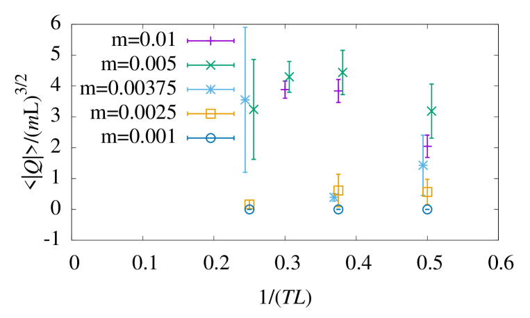
Figure 9: Finite size scaling of the chiral zero modes’ effect. Data at $T=220$ MeV are shown. The expected $L^{3/2}$ scaling of $\langle|Q|\rangle$ is saturated for $1/LT<0.4$.

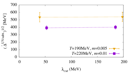
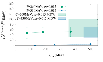
Figure 10: Cut-off $\lambda_{cut}$ dependence of $[\bar{\Delta}^{UVsubt.}]^{1/2}$. The left panel shows data at $T=190$ MeV and $220$ MeV and the right is for $T=260$ and 330 MeV. The lower three temperatures show a good saturation but the data at $T=330$ MeV is monotonically increasing and undershoot the band, which represents the stochastic estimates using the Möbius domain-wall Dirac operator.

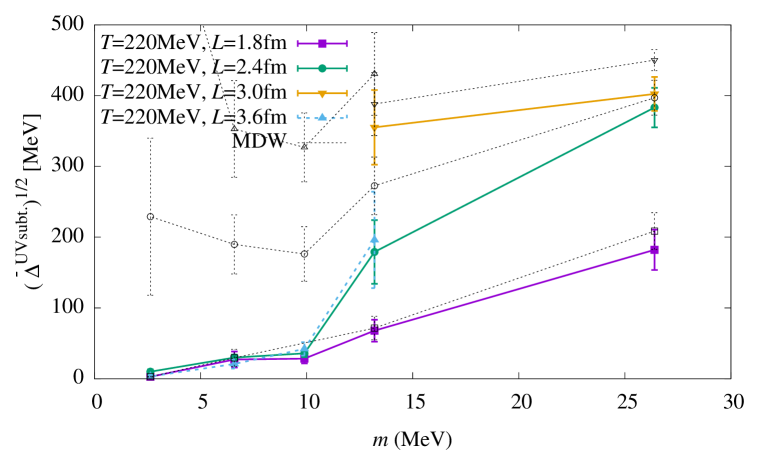
Figure 11: $[\bar{\Delta}^{UVsubt.}]^{1/2}$ as a function of $m$. Data at $T=220$ MeV with four different volumes are shown. at $T=220$ MeV are shown. Filled symbols with solid lines are data of reweighted overlap fermion, those with dashed lines are at $L=48$ whose statistics may be not good enough after the reweighting, and dotted open symbols are those of the Möbius domain-wall fermion.

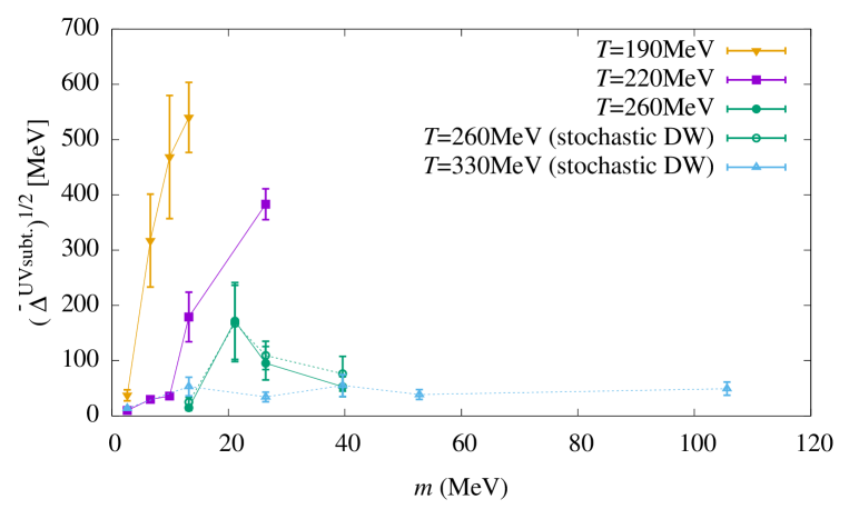
Figure 12: The same as Fig. 11 but at different temperatures.

$\beta$	$L^{3}\times L_{t}$	$T$(MeV)	$m$	$\rho(\lambda=0)$	$\langle Q^{2}\rangle$	$\bar{\Delta}^{UVsubt.}$
4.24	$32^{3}\times 12$	195	0.0025	0.00211(91)	0.084(37)
			0.005	0.0134(22)	0.575(83)
			0.01	0.0393(69)	3.1(10)
4.30	$32^{3}\times 14$	190	0.001	0.9(9)$\times 10^{-9}$	4(4)$\times 10^{-8}$	0.00020(11)
			0.0025	0.0037(11)	0.113(29)	0.0144(77)
			0.00375	0.0126(25)	0.69(17)	0.031(15)
			0.005	0.0113(19)	0.442(83)	0.0419(98)
	$32^{3}\times 12$	220	0.001	0.8(8)$\times 10^{-7}$	4(4)$\times 10^{-6}$	1.4(9)$\times 10^{-5}$
			0.0025	0.00035(22)	0.014(12)	0.000128(35)
			0.00375	0.000262(88)	0.0110(36)	0.000185(57)
			0.005	0.0064(14)	0.367(74)	0.0046(23)
			0.01	0.0160(22)	1.13(16)	0.0211(31)
	$32^{3}\times 10$	260	0.005	0.00104(76)	0.043(20)	3(2)$\times 10^{-5}$
			0.008	0.0031(11)	0.122(38)	0.0042(34)
			0.01	0.0047(13)	0.232(71)	0.00130(83)
			0.015	0.0057(22)	0.251(96)	0.00040(27)
	$32^{3}\times 8$	330	0.001	0(0)	0(0)	3(6)$\times 10^{-5}$
			0.005	1.2(9)$\times 10^{-5}$	0.00049(39)	0.00040(26)
			0.01	6(2)$\times 10^{-5}$	0.0024(14)	0.000169(87)
			0.015	0.00074(62)	0.044(28)	0.00043(31)
			0.02	0.0025(10)	0.099(41)	0.000215(99)
			0.04	0.0044(16)	0.508(97)	0.00035(17)

Table 2: The results for the lowest bin of the eigenvalue density or $\rho(\lambda=0)$, $\langle Q^{2}\rangle=\chi_{t}V$, and axial $U(1)$ susceptibility $\bar{\Delta}^{UVsubt.}$. For $T=330$ MeV, the stochastic Möbius domain-wall results are listed.

III.4 Meson correlators

In the previous subsection we studied the difference between the pseudoscalar and scalar two-point correlation function integrated over the whole lattice. Since we have subtracted the short-range UV divergent part, the quantity is essentially probing physics at the scale of our lattice size $L$, which is sensitive to the near zero modes. In this subsection, we investigate the mesonic two point correlation function itself, which must contain shorter-range information of QCD, as our fitting range is typically $L/4$.

We measure the spatial correlator in the $z$ direction

$$C_{\Gamma}(z)=-\sum_{x,y,t}\langle\mathcal{O}_{\Gamma}(x,y,z,t)\bar{\mathcal{O}}_{\Gamma}(0,0,0,0)\rangle,$$ (12)

with $\mathcal{O}_{\Gamma}=\bar{q}\vec{\tau}\Gamma q$. Here $\vec{\tau}$ are the generators in the flavor space. For $\Gamma$ we choose $\gamma_{5}$($PS$), $1$($S$), $\gamma_{1,2}$($V$), $\gamma_{5}\gamma_{1,2}$($A$), $\gamma_{4}\gamma_{3}$($T_{t}$) and $\gamma_{5}\gamma_{4}\gamma_{3}$($X_{t}$). In this work, we focus on $T_{t}$, and $X_{t}$ channels, which are related by the axial $U(1)$ transformation, as well as the $V$ and $A$ channels to check the recovery of the $SU(2)_{L}\times SU(2)_{R}$ symmetry. We find that the $S$ correlator is too noisy to extract the “mass” and compare it with that of $PS$. For other channels, we will report elsewhere.

Since this quantity represents shorter distance physics than the axial $U(1)$ susceptibility obtained from integration over whole lattice, the violation of the Ginsparg-Wilson relation enhanced by near-zero modes found in Tomiya:2016jwr is less severe. Therefore, we employ the Möbius domain-wall fermion formalism without reweighting. In order to improve the statistics, rotationally equivalent directions are averaged. Also, low-mode averaging Giusti:2004yp ; DeGrand:2004qw using 40 lowest eigenmodes of $H_{DW}(m)$ is performed with four equally spaced source points at temperature $T=220$ MeV.

For the channels other than $S$, the signal is good enough to extract the asymptotic behavior of $C_{\Gamma}(z)$ at large $z$, which should contain the information of the screening mass. However, the correlator at high temperatures may not behave like a single exponential even at large $z$. To circumvent this, recent studies often apply multi-state fits and introduce various source types to extract ground-state values, e.g. in Bazavov:2019www .

The asymptotic behavior depends on the structure of the spectral functions (in the spatial direction) for each channel $\Gamma$:

$$C_{\Gamma}(z)=\int d\omega\rho_{\Gamma}(\omega)\int\frac{dp_{z}}{2\pi}\frac{2\omega e^{ip_{z}z}}{p_{z}^{2}+\omega^{2}}=\int d\omega\rho_{\Gamma}(\omega)e^{-\omega z}.$$ (13)

When the spectral function $\rho_{\Gamma}(\omega)$ starts from a series of delta functions, which represents isolate poles, $C_{\Gamma}(z)$ at large $z$ is dominated by a single exponential. On the other hand, if the correlator is described by deconfined two quarks, $\rho_{\Gamma}(\omega)$ is a continuous function of $\omega$, provided that the volume is sufficiently large. Let us assume that $\rho_{\Gamma}(\omega)$ becomes nonzero at a threshold $2\bar{m}$, where $\bar{m}$ is a constituent screening quark mass. For large $z$, we can expand $\rho_{\Gamma}(\omega)$ as $\theta(\omega-2\bar{m})(c_{0}+c_{1}(\omega-2\bar{m})+\cdots)$ (with a step function $\theta$), which results in $C_{\Gamma}(z)\sim\exp(-2\bar{m}z)(c_{0}/z+O(1/z^{2}))$. In the Appendix A, we show that this form of the spectral function is indeed realized in the free two quark propagators. The essential difference from the single exponential is, thus, the factor $1/z$. In this study we therefore apply two types of fitting functions: the standard cosh function,

$$A_{\Gamma}\frac{\cosh(m_{\Gamma}(z-L/2))}{\sinh(m_{\Gamma}L/2)},$$ (14)

and the two-quark-inspired function (2q),

$$B_{\Gamma}\left(\frac{e^{-m^{\prime}_{\Gamma}z}}{m^{\prime}_{\Gamma}z}+\frac{e^{-m^{\prime}_{\Gamma}(L-z)}}{m^{\prime}_{\Gamma}(L-z)}\right).$$ (15)

In the free quark limit, we obtained more complete form of the two-quark propagations for each channel Rohrhofer:2017grg . Note that in this limit, $\bar{m}=\pi T$, which is the lowest Matsubara mass. It is, therefore, interesting to see how much $m^{\prime}_{\Gamma}$ is close to $2\pi T$ at our simulated temperature.

In order to compare the above fitting functions, it is helpful to plot their effective masses $m_{\Gamma}(z)$ and $m^{\prime}_{\Gamma}(z)$ defined as the solutions of

$$\frac{\cosh(m_{\Gamma}(z)(z-L/2))}{\cosh(m_{\Gamma}(z)(z+1-L/2))} = \frac{C_{\Gamma}(z)}{C_{\Gamma}(z+1)},$$ (16)

and

$$\frac{\frac{e^{-m^{\prime}_{\Gamma}(z)z}}{m^{\prime}_{\Gamma}(z)z}+\frac{e^{-m^{\prime}_{\Gamma}(z)(L-z)}}{m^{\prime}_{\Gamma}(z)(L-z)}}{\frac{e^{-m^{\prime}_{\Gamma}(z)(z+1)}}{m^{\prime}_{\Gamma}(z)(z+1)}+\frac{e^{-m^{\prime}_{\Gamma}(z)(L-z-1)}}{m^{\prime}_{\Gamma}(z)(L-z-1)}} = \frac{C_{\Gamma}(z)}{C_{\Gamma}(z+1)},$$ (17)

respectively, with the lattice data of $C_{\Gamma}(z)/C_{\Gamma}(z+1)$. If the fitting form is good, the effective mass converges to a constant at a shorter value of $z$. In Fig. 13, we plot typical effective mass plots at $T=220$ MeV. Square symbols are data for $m_{\Gamma}(z)$ and the circles are those for $m^{\prime}_{\Gamma}(z)$. The top two panels show the data obtained from $A$ correlators, while the bottom panels are from $T_{t}$ correlators. The left panels are at the heaviest simulated mass $m=0.01$ and the right ones are at the lightest $m=0.001$. The band indicates the fitting result and its range. We find that the 2q function shows longer and more stable plateux.

It is interesting to see that the plateaux are located at a mass lower than $2\pi T$ which is indicated by dashed lines. While we plan to give a detailed analysis in another publication JLQCD:2020 , we show the screening mass $m^{\prime}$ obtained by a fit to the 2q formula Eq. (15). The results are listed in Tab. 3.

In Fig. 15, we plot the difference of the fitted $m^{\prime}$ between $T_{t}$ and $X_{t}$ correlators at $T=220$ MeV at different volumes. They are connected by the $U(1)_{A}$ rotation, and therefore, the difference, denoted by $\Delta m_{\rm screen}$, is a probe of the axial $U(1)$ symmetry. For the reference, we also plot in Fig. 15 the results for the difference between $A$ and $V$ channels, which is an indicator for the $SU(2)_{L}\times SU(2)_{R}$ symmetry.

Although the $U(1)$ data at heavier quark masses are noisier than those for $SU(2)_{L}\times SU(2)_{R}$, their chiral limit looks consistent with zero, and the central values are only a few MeV, at the lightest quark mass. We note that their individual mass is $\sim 1$ GeV. Therefore, the axial $U(1)$ symmetry relation is satisfied at a sub-% level. This behavior is also seen at different temperatures, as shown in Fig. 16, except for $T=190$ MeV (but they are still consistent with zero with large error bars). The disappearance of the axial $U(1)$ anomaly is consistent with other observables obtained using the reweighted overlap fermions.

				$m^{\prime}$(MeV)
$\beta$	size	$T$(MeV)	$ma$	$PS$	$S$	$V$	$A$	$T_{t}$	$X_{t}$
4.30	$32^{3}\times 14$	190	0.001		172(104)	832(66)	872(62)	749(171)	1209(249)
			0.0025	44(41)		1015(216)	928(214)	802(100)	1020(129)
			0.00375	118(20)		747(61)	862(86)	1111(61)	759(125)
			0.005	147(24)		806(99)	923(151)	942(82)	1036(123)
	$24^{3}\times 12$	220	0.001	482(31)	482(32)	1027(41)	1028(41)	1088(22)	1086(22)
			0.0025	413(47)	510(64)	1074(91)	1078(92)	1015(94)	1166(108)
			0.00375	512(31)	590(59)	1055(44)	1068(46)	1138(35)	1108(31)
			0.005	386(39)	640(237)	1103(54)	1109(56)	1011(48)	1153(73)
			0.01	467(26)	772(104)	1070(53)	1040(60)	1093(24)	1160(29)
	$32^{3}\times 12$	220	0.001	433(56)	445(55)	1047(36)	1048(30)	1066(42)	1060(43)
			0.0025	486(25)	538(46)	1031(48)	1030(36)	1122(44)	1156(43)
			0.00375	402(28)	698(269)	978(65)	1006(63)	1024(52)	942(51)
			0.005	403(46)		1054(47)	1073(32)	1252(94)	1094(108)
			0.01	408(24)		967(51)	1062(39)	1128(52)	1096(59)
	$40^{3}\times 12$	220	0.005	334(85)		1022(37)	1021(37)	1068(69)	1146(45)
			0.01	375(35)		1000(21)	1040(33)	1056(55)	1228(77)
	$48^{3}\times 12$	220	0.001	569(35)	571(36)	1001(31)	1001(31)	1126(21)	1125(21)
			0.0025	608(21)	616(21)	1002(34)	1003(34)	1114(40)	1113(40)
			0.00375	577(66)	540(154)	944(51)	946(53)	992(66)	1045(76)
			0.005	425(62)	581(125)	1085(28)	1092(28)	1091(59)	1122(68)
	$32^{3}\times 10$	260	0.005	959(18)	998(20)	1307(7)	1308(7)	1368(7)	1366(7)
			0.008	941(19)	966(22)	1332(11)	1333(11)	1386(10)	1385(10)
			0.01	850(25)	997(69)	1313(11)	1314(11)	1357(15)	1363(14)
			0.015	935(50)	1144(90)	1381(13)	1387(14)	1426(14)	1436(15)
	$32^{3}\times 8$	330	0.001	1486(34)	1486(34)	1781(14)	1781(14)	1837(14)	1837(14)
			0.005	1535(13)	1535(13)	1799(9)	1799(9)	1849(11)	1849(11)
			0.01	1551(12)	1553(12)	1818(10)	1819(10)	1857(9)	1857(9)
			0.015	1526(11)	1528(11)	1792(10)	1793(10)	1853(11)	1854(11)
			0.02	1489(49)	1610(56)	1781(9)	1783(9)	1806(10)	1809(10)
			0.04	1560(19)	1574(20)	1833(12)	1838(12)	1864(11)	1870(11)

Table 3: Meson screening mass determined with two-quark-inspired fit ansatz. Fit range is several lattice spacings around $z=8$ (0.6 fm) depending on parameters.

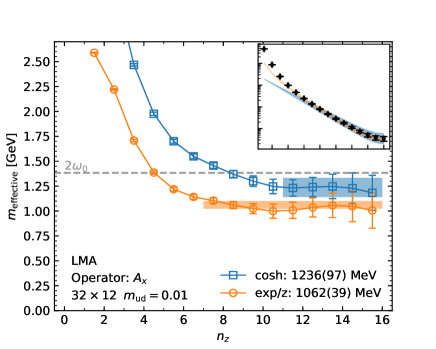
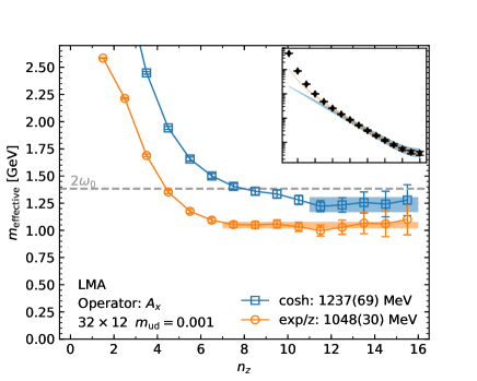
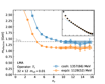
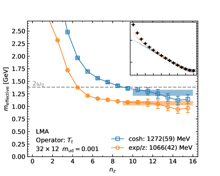
Figure 13: Cosh (squares) and “2-quark”(triangles) effective masses at $T=220$ MeV. The top panels show the data from $A$ correlators, while the bottom panels are $T_{t}$ correlators. The left panels are at the heaviest simulated mass $m=0.01$ and the right ones are at the lightest $m=0.001$. The band indicates the fit result and its range. The dashed line shows the Matsubara frequency $\pi T$ times 2 expected for two free quarks.

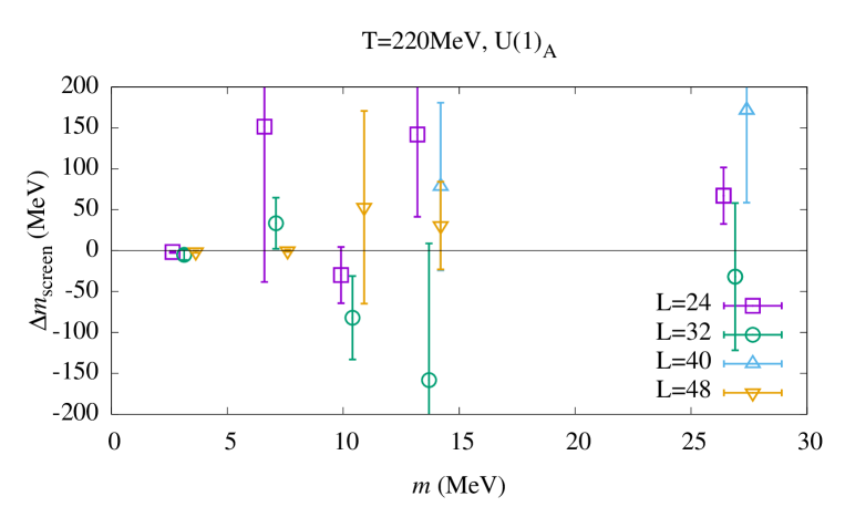
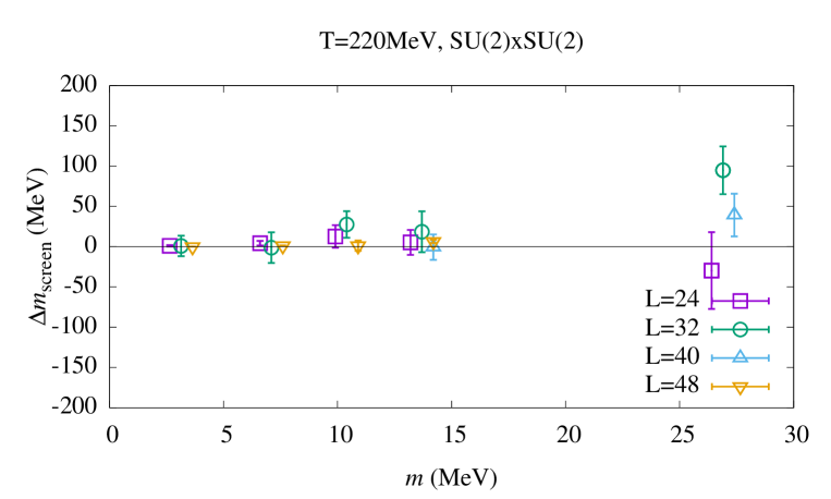
Figure 14: Difference of the fitted $m^{\prime}$ between $T_{t}$ and $X_{t}$ correlators, which are connected by the $U(1)_{A}$ rotation. The data at $T=220$ MeV at different volumes are shown.

Figure 15: The same as Fig. 15 but between $A$ and $V$ correlators, which shows the $SU(2)_{L}\times SU(2)_{R}$ symmetry.

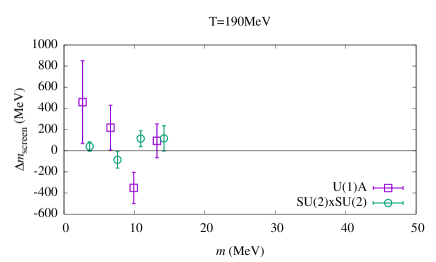
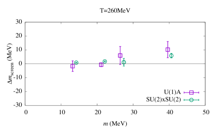
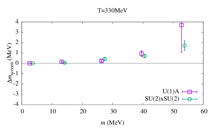
Figure 16: Difference of the fitted $m^{\prime}$ between $T_{t}$ and $X_{t}$ correlators (squares), and that between $A$ and $V$ correlators (circles).

III.5 Baryon correlators

Finally, let us discuss baryon correlators. We calculate the spatial correlation functions of baryon operators projected onto positive $z$-parity (or an even component under the $z$ reflection) and the lowest Matsubara frequency $\omega_{0}=\pi T$, which takes account of the anti-periodic boundary conditions in $t$-direction DeTar:1987xb :

$$C_{j}=\sum_{x,y,t}e^{it\omega_{0}}\langle N^{+}_{j}(x,y,z,t)\bar{N}^{+}_{j}(0,0,0,0)\rangle,$$ (18)

with nucleon operators $N^{+}_{j}=\hat{P}^{z}_{+}(q^{T}i\tau_{2}\Gamma_{j}^{1}q)\Gamma_{j}^{2}q$, and the parity projection operator $\hat{P}^{z}_{+}=(1+\gamma_{3})/2$. The combinations $(\Gamma_{j}^{1},\Gamma_{j}^{2})$ specify the operator channels: $N_{1}=(C\gamma_{5},1),N_{2}=(C,\gamma_{5}),N_{3}=(C\gamma_{4}\gamma_{5},1)$, and $N_{4}=(C\gamma_{4}\vec{\tau},\gamma_{5}\vec{\tau})$ with the charge conjugation matrix $C=i\gamma_{2}\gamma_{4}$. Similar to the case of mesons, $N_{1}$ and $N_{2}$ channels are related by the axial $U(1)$ transformation, and the $N_{3}$ – $N_{4}$ pair probes $SU(2)_{L}\times SU(2)_{R}$ symmetry Nagata:2007di .

Along the lines of the two-quark-inspired function for mesons, we use a three-quark-inspired function

$$B_{j}\frac{e^{-m^{\prime}_{j}z}}{m^{\prime}_{j}z^{2}}$$ (19)

to extract a screening mass $m^{\prime}_{j}$ for each channel by fitting the forward propagating states. This procedure gives qualitatively the same picture as in the previous section: a more stable plateau located at a lower energy value than that from the single $\cosh$ function. We therefore use $m^{\prime}$ to compare masses of different channels. Contrary to the case of mesons, we measure the baryon correlation functions exclusively in $z$-direction without low-mode averaging.

The numerical results presented in Table 4 and in Fig. 18 show the difference of $m^{\prime}$ between the axial $U(1)$ partners. While the uncertainty grows with increasing quark mass, the signal is consistent with zero for all volumes at $T=$220 MeV. A similar restoration pattern is seen for $SU(2)_{L}\times SU(2)_{R}$ symmetry, as shown in Fig. 18, albeit with less fluctuations.

In Fig. 19 the mass difference for pairs of both symmetries is shown at different temperatures. At $T=190$ MeV, closer to the chiral transition, noise dominates all quark masses except the lightest one. All data indicate consistency with zero in the chiral limit. At $T=260$ MeV and $T=330$ MeV some tiny violation at the order of $\mathcal{O}(10)$ MeV can be seen for non-vanishing quark masses. Similar to the meson screening masses, this is $\sim 1\%$ of the individual screening masses $m^{\prime}$.

				$m^{\prime}$(MeV)
$\beta$	size	$T$(MeV)	$ma$	$N_{1}$	$N_{2}$	$N_{3}$	$N_{4}$
4.30	$32^{3}\times 14$	190	0.001	628(227)	619(235)	723(245)	621(335)
			0.0025			1882(409)	1260(852)
			0.00375			1576(403)	1640(292)
			0.005			1173(348)	1410(150)
	$24^{3}\times 12$	220	0.001	1525(83)	1525(83)	1848(48)	1847(48)
			0.0025	1626(39)	1623(41)	1847(37)	1838(45)
			0.00375	1665(45)	1645(46)	1834(35)	1828(36)
			0.005	1351(100)	2291(500)	1863(72)	1745(79)
			0.01	1350(77)	1949(200)	1865(60)	1719(63)
	$32^{3}\times 12$	220	0.001	1563(49)	1572(49)	1700(35)	1697(36)
			0.0025	1440(48)	1484(60)	1647(49)	1640(49)
			0.00375	1507(81)	1469(103)	1687(41)	1687(39)
			0.005	1557(56)	1494(97)	1754(48)	1750(46)
			0.01	1343(95)	1854(160)	1763(50)	1645(50)
	$40^{3}\times 12$	220	0.005	1442(82)	1521(116)	1681(101)	1624(70)
			0.01	1425(93)	1459(166)	1692(52)	1673(44)
	$48^{3}\times 12$	220	0.001	1416(122)	1418(123)	1307(113)	1305(114)
			0.0025			1466(295)	1999(266)
			0.00375			1773(234)	1403(196)
			0.005	1605(56)	1620(50)	1716(59)	1643(52)
	$32^{3}\times 10$	260	0.005	2042(23)	2071(25)	2163(19)	2149(20)
			0.008	2018(32)	2020(32)	2160(29)	2154(29)
			0.01	1950(91)	1902(131)	2226(64)	2061(77)
			0.015	2080(44)	2114(53)	2207(43)	2196(40)
	$32^{3}\times 8$	330	0.001	2847(34)	2847(34)	2948(30)	2948(30)
			0.005	2727(38)	2728(38)	2835(39)	2833(39)
			0.01	2775(45)	2775(45)	2900(50)	2899(49)
			0.015	2773(19)	2776(19)	2873(17)	2869(17)
			0.02	2740(32)	2745(32)	2864(30)	2859(30)
			0.04	2710(28)	2733(30)	2857(23)	2841(22)

Table 4: Baryon screening masses determined with the three-quark-inspired fit ansatz.

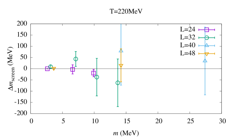
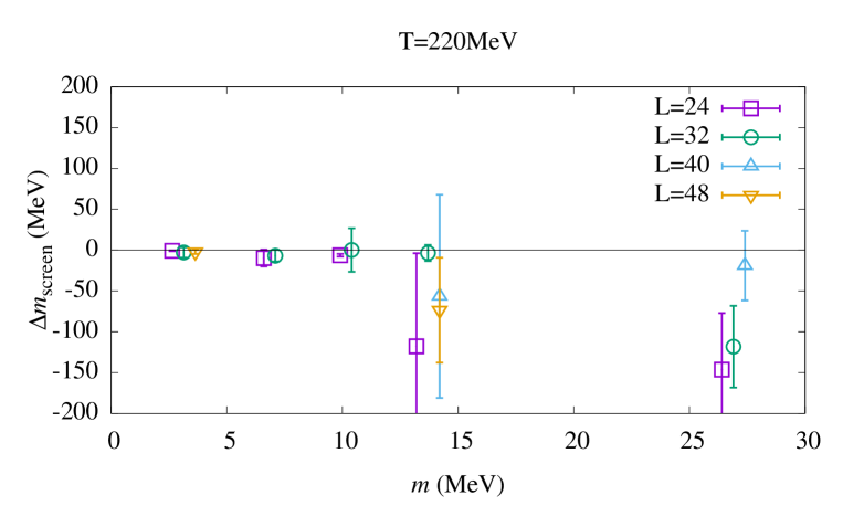
Figure 17: Difference of the fitted $m^{\prime}$ between the baryon $N_{1}$ and $N_{2}$ correlators, which are connected by the $U(1)_{A}$ rotation. The data at $T=220$ MeV at different volumes are shown.

Figure 18: The same as Fig. 18 but between the baryon $N_{3}$ and $N_{4}$ correlators, which shows the $SU(2)_{L}\times SU(2)_{R}$ symmetry.

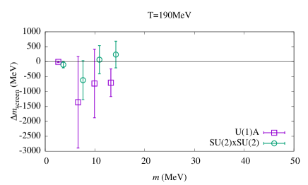
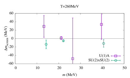
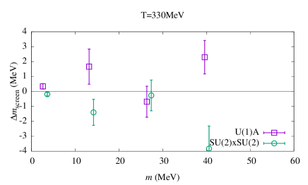
Figure 19: Difference of the fitted $m^{\prime}$ between the baryon $N_{1}$ and $N_{2}$ correlators (squares) and that between the baryon $N_{3}$ and $N_{4}$ correlators (circles).

IV Conclusion

In this work, we simulated two-flavor lattice QCD and tried to quantify how much of the axial $U(1)$ anomaly survives at high temperatures $190$–330 MeV. We employed the Möbius domain-wall fermion action and the overlap fermion action whose determinant is obtained by a stochastic reweighting technique. We fixed the lattice spacing to 0.074 fm, and chose more than four quark masses, including one below the physical point.

We confirmed that our data are consistent with those in the previous works Tomiya:2016jwr extending statistics of ensembles at $\beta=4.24$. We also observed a good consistency between the Möbius domain-wall and overlap fermions, except for the axial $U(1)$ susceptibility, which is very sensitive to the violation of the chiral symmetry at $T=220$ MeV. The discretization effect is therefore well under control. We also confirmed that the systematics due to finite size of the lattice is under control. Our data with various lattice sizes agree, except for those with $L=24$, which has a small aspect ratio $TL=2$ at $T=220$ MeV.

In the Dirac spectrum we found a strong suppression of low but non-zero eigenmodes. The higher temperature, the more suppression of the low lying modes observed. On the other hand, for the chiral zero mode, a peak is found at all four simulated temperatures but its quark mass dependence is steep and the chiral limit is consistent with zero.

As expected from the behavior of the chiral zero mode, a sharp disappearance of the topological susceptibility is found, which suggests a mass dependence starting with a power $\sim m^{4}$ near the chiral limit. Our numerical data for the axial U(1) susceptibility, meson and baryon correlators also indicate that the axial $U(1)$ anomaly is consistent with zero in the chiral limit. From these observations we conclude that the remaining anomaly of the axial $U(1)$ symmetry at the physical point for $T\geq$ 1.1 $T_{c}$ is at most a few MeV level, which is $\sim 1$% of the simulated temperatures.

To examine if the disappearance of the $U(1)_{A}$ anomaly occurs at the same time as the $SU(2)_{L}\times SU(2)_{R}$ symmetry is restored, we need a simulation around the critical temperature, which is beyond the scope of this paper.

Appendix A Spectral function of two and three non-interacting quarks

In this appendix, we compute propagators for two and three non-interacting quarks in $d$-dimensions (to show that $d=4$ is special). To take the finite temperature into account, the spacetime is assumed to be an Euclidean flat continuum space with one direction compactified. Namely, we consider $S^{1}\times\mathbb{R}^{d-1}$, and anti-periodic boundary conditions are imposed on the fermions. We denote the compact direction by $x_{0}$ and consider spatial propagators in the $x_{1}$ direction.

A.1 Two quarks

Let us start with the non-interacting pseudoscalar “meson” propagator, which is expressed by two massless and non-interacting quarks. By the standard Fourier transformation we obtain

$$C_{2q}(x_{1}) \equiv \int_{S^{1}\times\mathbb{R}^{d-2}}d^{d-1}x\langle\bar{d}\gamma_{5}u(x)\bar{u}\gamma_{5}d(0)\rangle$$ (20)

$$= \int_{S^{1}\times\mathbb{R}^{d-2}}d^{d-1}x{\rm tr}[\gamma_{5}D^{-1}(x,0)\gamma_{5}D^{-1}(0,x)]$$

$$= 4\int_{S^{1}\times\mathbb{R}^{d-2}}d^{d-1}x\int\frac{d^{d}p}{(2\pi)^{d}}\int\frac{d^{d}p^{\prime}}{(2\pi)^{d}}\frac{p^{\mu}p_{\mu}^{\prime}}{(p)^{2}(p^{\prime})^{2}}e^{i(p-p^{\prime})_{\nu}x^{\nu}}$$

$$= 4\int\frac{d^{d-1}\bm{p}}{(2\pi)^{d-1}}\int\frac{dp_{1}}{2\pi}\int\frac{dp^{\prime}_{1}}{2\pi}\frac{(p_{1}p^{\prime}_{1}+\bm{p}^{2})}{(p_{1}^{2}+\bm{p}^{2})(p_{1}^{\prime 2}+\bm{p}^{2})}e^{i(p_{1}-p_{1}^{\prime})x_{1}}.$$

Noting that the 0-th component of $\bm{p}$ denoted by $p_{0}$ is discrete, and neglecting higher $p_{0}$ contribution except for the lowest Matsubara frequency $p_{0}=M=\pm\pi T$, we can use the following approximation

$$\int\frac{d^{d-1}\bm{p}}{(2\pi)^{d-1}}\sim 2T\int\frac{d^{d-2}\bm{q}}{(2\pi)^{d-2}},\;\;\;\bm{p}^{2}=M^{2}+\bm{q}^{2},$$ (21)

where the $(d-2)$-dimensional vector $\bm{q}$ is given by $\bm{q}=(p_{2},p_{3},\cdots p_{d-1})$ and the factor two comes from the two possible signs of $M$. Changing the variables as $P_{1}=p_{1}-p^{\prime}_{1}$, $R_{1}=(p_{1}+p^{\prime}_{1})/2$ and explicitly integrating over $R_{1}$ and $P_{1}$, we obtain

$$C_{2q}(x_{1}) = 4T\int\frac{d^{d-2}\bm{q}}{(2\pi)^{d-2}}e^{-2\sqrt{M^{2}+\bm{q}^{2}}x_{1}}=4CT\int dqq^{d-3}e^{-2\sqrt{M^{2}+q^{2}}x_{1}}$$ (22)

$$= CT\int^{\infty}_{2M}d\omega\omega\left(\sqrt{\frac{\omega^{2}}{4}-M^{2}}\right)^{d-4}e^{-\omega x_{1}},$$

where the constant $C$ comes from the solid angle integral. In the last line we have changed the integral variable to $\omega=2\sqrt{M^{2}+q^{2}}$. Note that a fractional power is absent for $d=4$.

From the above integral, we can read off the spectral function for $d=4$ as

$$\rho_{2q}^{\rm free}(\omega)=2CT\theta(\omega-2M)\left[2M+(\omega-2M)\right],$$ (23)

which supports our assumption for the fitting form Eq. (15) of the meson correlators. Here we have chosen the pseudoscalar correlators but it was confirmed in Rohrhofer:2017grg by a full computation including higher Matsubara frequencies that this asymptotic form is universal in all other channels.

A.2 Three quarks

Next let us consider a “baryon” two-point function in which three non-interacting quarks propagate, choosing the $N_{1}$ channel,

$$\int_{S^{1}\times\mathbb{R}^{d-2}}d^{d-1}xe^{iMx_{0}}\langle[(u^{T}C\gamma_{5}d)u](x)[\bar{u}(\bar{d}C\gamma_{5}\bar{u}^{T}](0)\rangle.$$ (24)

One of the contractions leads to

$$C_{3q}(x_{1}) \equiv \int_{S^{1}\times\mathbb{R}^{d-2}}d^{d-1}xe^{iMx_{0}}D^{-1}(x,0){\rm tr}[\gamma_{5}D^{-1}(x,0)\gamma_{5}D^{-1}(0,x)]$$ (25)

$$= 4\int_{S^{1}\times\mathbb{R}^{d-2}}d^{d-1}x\int\frac{d^{d}p}{(2\pi)^{d}}\int\frac{d^{d}p^{\prime}}{(2\pi)^{d}}\int\frac{d^{d}p^{\prime\prime}}{(2\pi)^{d}}\frac{(p_{\mu}p^{\mu})(p^{\prime\prime}_{\nu}\gamma^{\nu})}{(p)^{2}(p^{\prime})^{2}(p^{\prime\prime})^{2}}e^{i(p-p^{\prime}-p^{\prime\prime})_{\nu}x^{\nu}+iMx_{0}}$$

$$= 4\int\frac{d^{d}p}{(2\pi)^{d}}\int\frac{d^{d}p^{\prime}}{(2\pi)^{d}}\int\frac{dp^{\prime\prime}_{1}}{(2\pi)}\frac{(p_{\mu}p^{\mu})(p^{\prime\prime}_{\nu}\gamma^{\nu})}{(p)^{2}(p^{\prime})^{2}(p^{\prime\prime})^{2}}e^{i(p-p^{\prime}-p^{\prime\prime})_{1}x_{1}},$$

where $p^{\prime\prime}_{\mu}=(p_{0}-p^{\prime}_{0}-M,p^{\prime\prime}_{1},\bm{q}-\bm{q}^{\prime})$ with $(d-2)$-momentum vectors $\bm{q}=(p_{2},p_{3},\cdots,p_{d-1})$ and $\bm{q}^{\prime}=(p^{\prime}_{2},p^{\prime}_{3},\cdots,p^{\prime}_{d-1})$. In the same way as the two-quark propagation, let us ignore the summation over $p_{0},p_{0}^{\prime}$ except for the three cases with $p_{0}-p_{0}^{\prime}-M=\pm M$. We then obtain

$$C_{3q}(x_{1}) \sim 12T^{2}\int\frac{d^{d-2}\bm{q}}{(2\pi)^{d-2}}\int\frac{d^{d-2}\bm{q}^{\prime}}{(2\pi)^{d-2}}\int\frac{dp_{1}}{(2\pi)}\int\frac{dp^{\prime}_{1}}{(2\pi)}\int\frac{dp^{\prime\prime}_{1}}{(2\pi)}$$ (26)

$$\frac{(p_{1}p^{\prime}_{1}+M^{2}+\bm{q}\cdot\bm{q}^{\prime})(p^{\prime\prime}_{1}\gamma_{1}+M\gamma_{0}+(\bm{q}-\bm{q}^{\prime})\cdot\bm{\gamma})}{(p_{1}^{2}+M^{2}+\bm{q}^{2})(p_{1}^{\prime 2}+M^{2}+\bm{q^{\prime}}^{2})(p_{1}^{{}^{\prime\prime}2}+M^{2}+(\bm{q}-\bm{q}^{\prime})^{2})}e^{i(p-p^{\prime}-p^{\prime\prime})_{1}x_{1}}$$

$$= \frac{3T^{2}}{2}\int\frac{d^{d-2}\bm{q}}{(2\pi)^{d-2}}\int\frac{d^{d-2}\bm{q}^{\prime}}{(2\pi)^{d-2}}e^{-(\sqrt{M^{2}+\bm{q}^{2}}+\sqrt{M^{2}+\bm{q^{\prime}}^{2}}+\sqrt{M^{2}+(\bm{q}-\bm{q}^{\prime})^{2}})x_{1}}$$

$$\times{\textstyle\frac{(\sqrt{M^{2}+\bm{q}^{2}}\sqrt{p_{1}^{\prime 2}+M^{2}+\bm{q^{\prime}}^{2}}+M^{2}+\bm{q}\cdot\bm{q}^{\prime})(\sqrt{p_{1}^{{}^{\prime\prime}2}+M^{2}+(\bm{q}-\bm{q}^{\prime})^{2}}\gamma_{1}+M\gamma_{0}+(\bm{q}-\bm{q}^{\prime})\cdot\bm{\gamma})}{\sqrt{M^{2}+\bm{q}^{2}}\sqrt{p_{1}^{\prime 2}+M^{2}+\bm{q^{\prime}}^{2}}\sqrt{p_{1}^{{}^{\prime\prime}2}+M^{2}+(\bm{q}-\bm{q}^{\prime})^{2}}}}.$$

As large $\bm{q}^{2},\bm{q}^{\prime 2}$ contributions are exponentially suppressed, let us expand the integrand with $\bm{q}^{2}/M$ and $\bm{q^{\prime}}^{2}/M$ so that the integral is greatly simplified as

$$C_{3q}(x_{1}) \sim 3T^{2}\int\frac{d^{d-2}\bm{q}}{(2\pi)^{d-2}}\int\frac{d^{d-2}\bm{q}^{\prime}}{(2\pi)^{d-2}}(\gamma_{1}+\gamma_{0})e^{-x_{1}(3M+(\bm{q}^{2}+\bm{q^{\prime}}^{2}-\bm{q}\cdot\bm{q^{\prime}})/M)}$$ (27)

$$\propto T^{2}\int_{0}^{\infty}dpp^{d-3}\left(\frac{M}{x_{1}}\right)^{(d-2)/2}e^{-3x_{1}(M+p^{2}/4M)}$$

$$\propto T^{2}\int_{3M}^{\infty}d\omega M^{d-2}(\omega-3M)^{\frac{d-4}{2}}x_{1}^{-\frac{d-2}{2}}e^{-\omega x_{1}}$$

$$\propto T^{2}\int_{3M}^{\infty}d\omega M^{d-2}(\omega-3M)^{d-3}e^{-\omega x_{1}},$$

where the integration over $\bm{q}^{\prime}-\bm{p}/2$ and solid angle in $\bm{q}$ are performed and an unimportant overall dimensionless (matrix-valued) constant is neglected.

From the above integral, we can read off the spectral function for $d=4$ as

$$\rho_{3q}^{\rm free}(\omega)=DT^{4}\theta(\omega-3M)(\omega-3M),$$ (28)

with a constant (matrix) $D$, which supports the asymptotic three-quark form $\exp(-3Mx_{1})/x_{1}^{2}$ corresponding to Eq. (19).

References

- (1) H. Itoyama and A. H. Mueller, “The Axial Anomaly at Finite Temperature,” Nucl. Phys. B 218, 349 (1983) doi:10.1016/0550-3213(83)90370-X.
- (2) T. D. Cohen, “QCD inequalities, the high temperature phase of QCD, and U(1)Asymmetry,” Phys. Rev. D 54, R1867 (1996) doi:10.1103/PhysRevD.54.R1867 [hep-ph/9601216].
- (3) T. D. Cohen, “The Spectral density of the Dirac operator above T(c),” nucl-th/9801061.
- (4) T. Banks and A. Casher, “Chiral Symmetry Breaking in Confining Theories,” Nucl. Phys. B 169, 103 (1980) doi:10.1016/0550-3213(80)90255-2.
- (5) S. Aoki, H. Fukaya and Y. Taniguchi, “Chiral symmetry restoration, eigenvalue density of Dirac operator and axial U(1) anomaly at finite temperature,” Phys. Rev. D 86, 114512 (2012) doi:10.1103/PhysRevD.86.114512 [arXiv:1209.2061 [hep-lat]].
- (6) R. D. Pisarski and F. Wilczek, “Remarks on the Chiral Phase Transition in Chromodynamics,” Phys. Rev. D 29, 338 (1984) doi:10.1103/PhysRevD.29.338.
- (7) D. Horvatić, D. Kekez and D. Klabučar, “ and mesons at high T when the (1) and chiral symmetry breaking are tied,” Phys. Rev. D 99, no. 1, 014007 (2019) doi:10.1103/PhysRevD.99.014007 [arXiv:1809.00379 [hep-ph]].
- (8) S. D. Bass and P. Moskal, “ and mesons with connection to anomalous glue,” Rev. Mod. Phys. 91, no. 1, 015003 (2019) doi:10.1103/RevModPhys.91.015003 [arXiv:1810.12290 [hep-ph]].
- (9) A. Gómez Nicola, J. Ruiz De Elvira and A. Vioque-Rodríguez, “The QCD topological charge and its thermal dependence: the role of the ,” JHEP 1911, 086 (2019) doi:10.1007/JHEP11(2019)086 [arXiv:1907.11734 [hep-ph]].
- (10) K. Yonekura, “Anomaly matching in QCD thermal phase transition,” JHEP 1905, 062 (2019) doi:10.1007/JHEP05(2019)062 [arXiv:1901.08188 [hep-th]].
- (11) A. Pelissetto and E. Vicari, “Relevance of the axial anomaly at the finite-temperature chiral transition in QCD,” Phys. Rev. D 88, no. 10, 105018 (2013) doi:10.1103/PhysRevD.88.105018 [arXiv:1309.5446 [hep-lat]].
- (12) Y. Nakayama and T. Ohtsuki, “Bootstrapping phase transitions in QCD and frustrated spin systems,” Phys. Rev. D 91, no. 2, 021901 (2015) doi:10.1103/PhysRevD.91.021901 [arXiv:1407.6195 [hep-th]].
- (13) T. Kanazawa and N. Yamamoto, “Quasi-instantons in QCD with chiral symmetry restoration,” Phys. Rev. D 91, 105015 (2015) doi:10.1103/PhysRevD.91.105015 [arXiv:1410.3614 [hep-th]].
- (14) T. Sato and N. Yamada, “Linking to model via decoupling,” Phys. Rev. D 91, no. 3, 034025 (2015) doi:10.1103/PhysRevD.91.034025 [arXiv:1412.8026 [hep-lat]].
- (15) Y. Nakayama and T. Ohtsuki, “Conformal Bootstrap Dashing Hopes of Emergent Symmetry,” Phys. Rev. Lett. 117, no. 13, 131601 (2016) doi:10.1103/PhysRevLett.117.131601 [arXiv:1602.07295 [cond-mat.str-el]].
- (16) A. Alexandru and I. Horváth, “Possible new phase of thermal QCD” Phys. Rev. D 100, no. 9, 094507 (2019) doi:10.1103/PhysRevD.100.094507 [arXiv:1906.08047 [hep-lat]].
- (17) E. Berkowitz, M. I. Buchoff and E. Rinaldi, “Lattice QCD input for axion cosmology,” Phys. Rev. D 92, no. 3, 034507 (2015) doi:10.1103/PhysRevD.92.034507 [arXiv:1505.07455 [hep-ph]].
- (18) R. Kitano and N. Yamada, “Topology in QCD and the axion abundance,” JHEP 1510, 136 (2015) doi:10.1007/JHEP10(2015)136 [arXiv:1506.00370 [hep-ph]].
- (19) C. Bonati, M. D’Elia, M. Mariti, G. Martinelli, M. Mesiti, F. Negro, F. Sanfilippo and G. Villadoro, “Axion phenomenology and -dependence from lattice QCD,” JHEP 1603, 155 (2016) doi:10.1007/JHEP03(2016)155 [arXiv:1512.06746 [hep-lat]].
- (20) P. Petreczky, H. P. Schadler and S. Sharma, “The topological susceptibility in finite temperature QCD and axion cosmology,” Phys. Lett. B 762, 498 (2016) doi:10.1016/j.physletb.2016.09.063 [arXiv:1606.03145 [hep-lat]].
- (21) S. Borsanyi et al., “Calculation of the axion mass based on high-temperature lattice quantum chromodynamics,” Nature 539, no. 7627, 69 (2016) doi:10.1038/nature20115 [arXiv:1606.07494 [hep-lat]].
- (22) F. Burger, E. M. Ilgenfritz, M. P. Lombardo and A. Trunin, “Chiral observables and topology in hot QCD with two families of quarks,” Phys. Rev. D 98, no. 9, 094501 (2018) doi:10.1103/PhysRevD.98.094501 [arXiv:1805.06001 [hep-lat]].
- (23) M. P. Lombardo and A. Trunin, “Topology and axions in QCD,” Int. J. Mod. Phys. A 35, no.20, 2030010 (2020) doi:10.1142/S0217751X20300100 [arXiv:2005.06547 [hep-lat]].
- (24) A. Bazavov et al. [HotQCD Collaboration], “The chiral transition and symmetry restoration from lattice QCD using Domain Wall Fermions,” Phys. Rev. D 86, 094503 (2012) doi:10.1103/PhysRevD.86.094503 [arXiv:1205.3535 [hep-lat]].
- (25) G. Cossu, S. Aoki, H. Fukaya, S. Hashimoto, T. Kaneko, H. Matsufuru and J.-I. Noaki, “Finite temperature study of the axial U(1) symmetry on the lattice with overlap fermion formulation,” Phys. Rev. D 87, no. 11, 114514 (2013) Erratum: [Phys. Rev. D 88, no. 1, 019901 (2013)] doi:10.1103/PhysRevD.88.019901, 10.1103/PhysRevD.87.114514 [arXiv:1304.6145 [hep-lat]].
- (26) M. I. Buchoff et al., “QCD chiral transition, U(1)A symmetry and the dirac spectrum using domain wall fermions,” Phys. Rev. D 89, no. 5, 054514 (2014) doi:10.1103/PhysRevD.89.054514 [arXiv:1309.4149 [hep-lat]].
- (27) T. W. Chiu et al. [TWQCD Collaboration], “Chiral symmetry and axial U(1) symmetry in finite temperature QCD with domain-wall fermion,” PoS LATTICE 2013, 165 (2014) doi:10.22323/1.187.0165 [arXiv:1311.6220 [hep-lat]].
- (28) G. Cossu et al. [JLQCD Collaboration], “Violation of chirality of the Möbius domain-wall Dirac operator from the eigenmodes,” Phys. Rev. D 93, no. 3, 034507 (2016) doi:10.1103/PhysRevD.93.034507 [arXiv:1510.07395 [hep-lat]].
- (29) G. Cossu and S. Hashimoto, “Anderson Localization in high temperature QCD: background configuration properties and Dirac eigenmodes,” JHEP 1606, 056 (2016) doi:10.1007/JHEP06(2016)056 [arXiv:1604.00768 [hep-lat]].
- (30) A. Tomiya, G. Cossu, S. Aoki, H. Fukaya, S. Hashimoto, T. Kaneko and J. Noaki, “Evidence of effective axial U(1) symmetry restoration at high temperature QCD,” Phys. Rev. D 96, no. 3, 034509 (2017) Addendum: [Phys. Rev. D 96, no. 7, 079902 (2017)] doi:10.1103/PhysRevD.96.034509, 10.1103/PhysRevD.96.079902 [arXiv:1612.01908 [hep-lat]].
- (31) V. Dick, F. Karsch, E. Laermann, S. Mukherjee and S. Sharma, “Microscopic origin of symmetry violation in the high temperature phase of QCD,” Phys. Rev. D 91, no. 9, 094504 (2015) doi:10.1103/PhysRevD.91.094504 [arXiv:1502.06190 [hep-lat]].
- (32) S. Sharma [HotQCD Collaboration], “The fate of and topological features of QCD at finite temperature,” arXiv:1801.08500 [hep-lat].
- (33) L. Mazur, O. Kaczmarek, E. Laermann and S. Sharma, “The fate of axial U(1) in 2+1 flavor QCD towards the chiral limit,” PoS LATTICE 2018, 153 (2019) doi:10.22323/1.334.0153 [arXiv:1811.08222 [hep-lat]].
- (34) B. B. Brandt, A. Francis, H. B. Meyer, O. Philipsen, D. Robaina and H. Wittig, “On the strength of the anomaly at the chiral phase transition in QCD,” JHEP 1612, 158 (2016) doi:10.1007/JHEP12(2016)158 [arXiv:1608.06882 [hep-lat]].
- (35) K.-I. Ishikawa, Y. Iwasaki, Y. Nakayama and T. Yoshie, “Nature of chiral phase transition in two-flavor QCD,” arXiv:1706.08872 [hep-lat].
- (36) B. B. Brandt, O. Philipsen, M. Cè, A. Francis, T. Harris, H. B. Meyer and H. Wittig, “Testing the strength of the anomaly at the chiral phase transition in two-flavour QCD,” PoS CD2018, 055 (2019) doi:10.22323/1.317.0055 [arXiv:1904.02384 [hep-lat]].
- (37) A. Bazavov et al., “Meson screening masses in (2+1)-flavor QCD,” Phys. Rev. D 100, no. 9, 094510 (2019) doi:10.1103/PhysRevD.100.094510 [arXiv:1908.09552 [hep-lat]].
- (38) H. T. Ding, S. T. Li, S. Mukherjee, A. Tomiya, X. D. Wang and Y. Zhang, “Correlated Dirac eigenvalues and axial anomaly in chiral symmetric QCD,” [arXiv:2010.14836 [hep-lat]].
- (39) S. Aoki et al. [JLQCD Collaboration], “Topological Susceptibility in QCD at Finite Temperature,” EPJ Web Conf. 175, 07024 (2018) doi:10.1051/epjconf/201817507024 [arXiv:1711.07537 [hep-lat]].
- (40) K. Suzuki et al. [JLQCD Collaboration], “Axial symmetry at high temperature in 2-flavor lattice QCD,” EPJ Web Conf. 175, 07025 (2018) doi:10.1051/epjconf/201817507025 [arXiv:1711.09239 [hep-lat]].
- (41) H. Fukaya [JLQCD Collaboration], “Can axial U(1) anomaly disappear at high temperature?,” EPJ Web Conf. 175, 01012 (2018) doi:10.1051/epjconf/201817501012 [arXiv:1712.05536 [hep-lat]].
- (42) K. Suzuki et al. [JLQCD Collaboration], “Axial U(1) symmetry and Dirac spectra in high-temperature phase of lattice QCD,” PoS LATTICE 2018, 152 (2018) doi:10.22323/1.334.0152 [arXiv:1812.06621 [hep-lat]].
- (43) K. Suzuki et al. [JLQCD Collaboration], “Axial U(1) symmetry, topology, and Dirac spectra at high temperature in lattice QCD,” PoS CD2018, 085 (2019) doi:10.22323/1.317.0085 [arXiv:1908.11684 [hep-lat]].
- (44) C. Rohrhofer, Y. Aoki, G. Cossu, H. Fukaya, C. Gattringer, L. Y. Glozman, S. Hashimoto, C. B. Lang and K. Suzuki, “Symmetries of the Light Hadron Spectrum in High Temperature QCD,” PoS LATTICE2019, 227 (2020) doi:10.22323/1.363.0227 [arXiv:1912.00678 [hep-lat]].
- (45) K. Suzuki et al. [JLQCD Collaboration], “Axial U(1) symmetry and mesonic correlators at high temperature in lattice QCD,” PoS LATTICE2019, 178 (2020) doi:10.22323/1.363.0178 [arXiv:2001.07962 [hep-lat]].
- (46) C. Rohrhofer, Y. Aoki, G. Cossu, H. Fukaya, L. Y. Glozman, S. Hashimoto, C. B. Lang and S. Prelovsek, “Approximate degeneracy of spatial correlators in high temperature QCD,” Phys. Rev. D 96, no. 9, 094501 (2017) Erratum: [Phys. Rev. D 99, no. 3, 039901 (2019)] doi:10.1103/PhysRevD.96.094501, 10.1103/PhysRevD.99.039901 [arXiv:1707.01881 [hep-lat]].
- (47) L. Y. Glozman, “Chiralspin symmetry and QCD at high temperature,” Eur. Phys. J. A 54, no. 7, 117 (2018) doi:10.1140/epja/i2018-12560-0 [arXiv:1712.05168 [hep-ph]].
- (48) C. B. Lang, “Low lying eigenmodes and meson propagator symmetries,” Phys. Rev. D 97, no. 11, 114510 (2018) doi:10.1103/PhysRevD.97.114510, [arXiv:1803.08693 [hep-ph]].
- (49) C. Rohrhofer et al., “Symmetries of spatial meson correlators in high temperature QCD,” Phys. Rev. D 100, no. 1, 014502 (2019) doi:10.1103/PhysRevD.100.014502 [arXiv:1902.03191 [hep-lat]].
- (50) G. Cossu, J. Noaki, S. Hashimoto, T. Kaneko, H. Fukaya, P. A. Boyle and J. Doi, “JLQCD IroIro++ lattice code on BG/Q,” [arXiv:1311.0084 [hep-lat]].
- (51) P. Boyle, A. Yamaguchi, G. Cossu and A. Portelli, “Grid: A next generation data parallel C++ QCD library,” [arXiv:1512.03487 [hep-lat]].
- (52) S. Ueda, S. Aoki, T. Aoyama, K. Kanaya, H. Matsufuru, S. Motoki, Y. Namekawa, H. Nemura, Y. Taniguchi and N. Ukita, “Development of an object oriented lattice QCD code ’Bridge++’,” J. Phys. Conf. Ser. 523, 012046 (2014) doi:10.1088/1742-6596/523/1/012046
- (53) M. Luscher and P. Weisz, “Computation of the Action for On-Shell Improved Lattice Gauge Theories at Weak Coupling,” Phys. Lett. 158B, 250 (1985) doi:10.1016/0370-2693(85)90966-9.
- (54) D. B. Kaplan, “A Method for simulating chiral fermions on the lattice,” Phys. Lett. B 288, 342 (1992) doi:10.1016/0370-2693(92)91112-M [hep-lat/9206013].
- (55) R. C. Brower, H. Neff and K. Orginos, “Mobius fermions,” Nucl. Phys. Proc. Suppl. 153, 191 (2006) doi:10.1016/j.nuclphysbps.2006.01.047 [hep-lat/0511031].
- (56) R. C. Brower, H. Neff and K. Orginos, “The Möbius domain wall fermion algorithm,” Comput. Phys. Commun. 220, 1 (2017) doi:10.1016/j.cpc.2017.01.024 [arXiv:1206.5214 [hep-lat]].
- (57) H. Neuberger, “Exactly massless quarks on the lattice,” Phys. Lett. B 417, 141 (1998) doi:10.1016/S0370-2693(97)01368-3 [hep-lat/9707022].
- (58) C. Morningstar and M. J. Peardon, “Analytic smearing of SU(3) link variables in lattice QCD,” Phys. Rev. D 69, 054501 (2004) doi:10.1103/PhysRevD.69.054501 [hep-lat/0311018].
- (59) R. Sommer, “Scale setting in lattice QCD,” PoS LATTICE 2013, 015 (2014) doi:10.22323/1.187.0015 [arXiv:1401.3270 [hep-lat]].
- (60) G. Cossu, H. Fukaya, S. Hashimoto, T. Kaneko and J. I. Noaki, “Stochastic calculation of the Dirac spectrum on the lattice and a determination of chiral condensate in 2+1-flavor QCD,” PTEP 2016, no.9, 093B06 (2016) doi:10.1093/ptep/ptw129 [arXiv:1607.01099 [hep-lat]].
- (61) L. Giusti, P. Hernandez, M. Laine, P. Weisz and H. Wittig, “Low-energy couplings of QCD from current correlators near the chiral limit,” JHEP 04, 013 (2004) doi:10.1088/1126-6708/2004/04/013 [arXiv:hep-lat/0402002 [hep-lat]].
- (62) T. A. DeGrand and S. Schaefer, “Improving meson two point functions in lattice QCD,” Comput. Phys. Commun. 159, 185-191 (2004) doi:10.1016/j.cpc.2004.02.006 [arXiv:hep-lat/0401011 [hep-lat]].
- (63) JLQCD Collaboration, in preparation
- (64) C. E. Detar and J. B. Kogut, “Measuring the Hadronic Spectrum of the Quark Plasma,” Phys. Rev. D 36, 2828 (1987) doi:10.1103/PhysRevD.36.2828.
- (65) K. Nagata, A. Hosaka and V. Dmitrasinovic, “Chiral properties of baryon interpolating fields,” Mod. Phys. Lett. A 23, 2381-2384 (2008) doi:10.1142/S0217732308029423 [arXiv:0705.1896 [hep-ph]].