Causal inference in absence of positivity: the role of overlap weights

Abstract

[Summary] What do we do when violations of the positivity assumption are expected? Several possible solutions exist in the literature. We consider propensity score (PS) methods that are commonly used in observational studies to assess causal treatment effects when the positivity assumption is violated. We focus on and examine four specific alternative solutions to the inverse probability weighting (IPW) trimming and truncation: matching weight (MW), Shannon’s entropy weight (EW), overlap weight (OW) and beta weight (BW) estimators.

In this paper, we demonstrate that these estimators target the same population of interest, the population of patients for whom we have sufficient PS overlap, i.e., where lies clinical equipoise. Then, we establish the nexus among the different corresponding weights (and estimators); this allows us to highlight the share properties and theoretical implications of these estimators. Finally, we introduce their augmented estimators that take advantage of estimating both the propensity score and regression models to enhance the treatment effect estimators in terms of bias and efficiency. We also elucidate the role of OW estimator as the flagship of all these methods that target the overlap population.

Our analytic results demonstrate that OW, MW, and EW are preferable when there is a moderate or extreme violations of the positivity assumption. We then evaluate, compare, and confirm their finite-sample performance of the aforementioned estimators via Monte Carlo simulations. Finally, we illustrate these methods using two real-world data examples marked by expected violations of the positivity assumption.

1 Introduction

A well-designed and well-executed randomized clinical trial (RCT)—with a perfect randomization, large sample size, full adherence, no attrition and no measurement error—is gold standard for causal inference since it leads to comparable treatment groups with respect to both measured and unmeasured covariates. Randomization ensures the comparability between the treatment groups where participants are enrolled based on clearly defined and objective eligibility criteria, which are embedded in the study protocol. Any difference in patients’ baseline covariates between treatment groups is random and their distributions coincide on average, which affords the study its internal validity.¹ This allows a straightforward assessment of the treatment effect: association is causation. More often physicians and investigators in such a trial operate, at least in principle, under the ideal of clinical equipoise, i.e., they would be a priori genuinely uncertain (from a historical or general practice perspective) about the therapeutic merits and the effectiveness of each treatment option.²As a result, randomization ensures positivity, i.e., each study participant has a chance of being assigned to either treatment option.

Unfortunately, it is not always feasible to conduct a randomized clinical trial for practical reasons, ethical concerns, or financial constraints. Furthermore, when feasible, strict eligibility criteria of an RCT do not always allow investigators to adequately enroll patients that are representative of the whole target population to which the treatment of interest, based on its intended purposes, will eventually be applied. For instance, it is well documented that older patients, higher risk patients, women, and patients from racial/ethnic minority groups are often underrepresented in RCTs.¹ Finally, despite their high quality, data from an RCT may not reflect those from a real-world evidence practice since the available hospital resources, logistics, and personnel as well as the treatment effectiveness may be drastically different in tightly-controlled confines of an RCT than in regular day-to-day clinical practice. Therefore, for a number of questions of interest arising in biomedical research, we often resort to observational studies for answers.

Unlike in RCTs, the treatment assignment is not random and usually beyond the investigators’ control in observational studies. Treatment options are either self-selected by patients (via some health-seeking behaviors) or recommended by their physicians following specific diagnosis or outcome prognosis. In most clinical practice, the treatment is assigned based on a range of deciding factors, including patient’s demographics, diagnosis, lab values, prognosis, provider’s preference, practice patterns, and even hospital characteristics (or capabilities). Hence, observational studies can be potentially marred by confounding, which is susceptible to jointly influence the treatment a patient can received and his or her final outcome. In addition, there is a number of potential study-altering factors (e.g., endogeneity, selection bias, collider bias, compliance) we need to sleuth on if we want to conduct a rigorous and reliable study.³ Nevertheless, principled design and analysis of observational studies are conducted with the objective of emulating a randomized clinical trial. ^{4, 5, 6, 7, 8, 9, 10} The goal of causal inference methods is thus to make the treatment groups comparable with respect to the distributions of their baseline covariates. Therefore, estimating the effects of treatment requires that we rule out any confounding due to systematic difference in the distributions of the baseline covariates that may explain the difference in outcome between treatment groups.

For many observational studies, propensity score (PS) methods are used to balance the distributions of the measured covariates, reduce or eliminate selection bias, emulate an RCT-like design, and evaluate the treatment effect. The propensity score is the conditional probability of treatment assignment, given the baseline covariates. It contains all measured information relevant for the treatment–outcome relationship. Furthermore, the PS has the balancing property, i.e., condition on the propensity score, the underlying distributions of covariates of the treatment groups are similar: the PS restores balance between these groups. ^{11, 12} At the heart of all propensity score methods are two fundamental assumptions: unconfoundness and positivity. For the unconfoundness assumption to be deemed acceptable, we assume that an extensive set of relevant and important covariates that are related to the treatment or the outcome of interest has been measured based on subject-matter expertise and can be used to remove or at least reduce confounding. Therefore, condition on the measured covariates, the study is considered as good as if it were a randomized clinical trial (with respect to the treatment assignment).

Once the selection of covariates is done, an important task is thus to ensure that the positivity (or experimental treatment assignment) assumption is satisfied: the propensity score must be bounded away from 0 and 1, given the smallest subset of covariates that make the uncounfoundness assumption valid. When satisfied, the positivity assumption guarantees that there is an appropriate overlap in the measured covariate distributions across the treatment groups. It ensures comparability of treated and control participants, i.e., some measured covariates do not deterministically lead to a specific treatment group (but not the other). Moreover, it helps avoid extrapolation beyond the common overlap region of the covariate distributions where we can reliably estimate the treatment effect. Along with the unconfoundness assumption, the positivity assumption implies that participants from one treatment group can always be used as good proxies (to infer potential outcomes) for the other group. This allows us to leverage the outcomes of treated (resp. untreated) participants to infer the potential outcomes of untreated (resp. treated) participants had they been treated (resp. untreated). Whenever the distributions of the covariates between the two treatment groups are drastically different, this may result in limited overlap of the distribution the propensity scores and violations (or near violations) of the positivity assumption. We will refer to violations or near violations of the positivity assumptions as lack of adequate positivity, as defined by Cheng et al.¹³

1.1 Lack of adequate positivity in observational studies

Different propensity score methods are affected differently by insufficient overlap in the distribution of the propensity scores or by the lack of adequate positivity and, hence, have different requirements. Note that in practice, overlap refers to how well the histograms of propensity scores in each treatment group cover (i.e., overlap with) each other. As opposed to propensity score matching and propensity stratification methods where a good overlap is a must to the success of their implementations, inverse probability weighting (IPW) methods do not impose strict requirements for good overlap of the distributions of the propensity scores per se. The main idea behind weighting methods is to create a pseudo-population, i.e., the target population of interest where, on average, the treatment groups are balanced with respect to their baseline covariates.^{14, 15} They usually lead to adequate covariate balance, sometimes even when there is limited overlap of the distribution of the propensity scores (see, for instance, the Lalonde data set in Ridgeway et al. ¹⁶). Nevertheless, a scrupulous evaluation of the common support has a fundamental implication: it allows us to speculate whether causal inference is advisable, i.e. whether the treatment groups overlap sufficiently well enough to provide reliable and stable estimate of the treatment effect. ^{17, 18, 19}

For inverse propensity score weighting (IPW) methods, lack of adequate positivity or insufficient overlap in the distribution of propensity scores may result in observations with propensity scores near 0 or 1 and lead to extreme weights. When that is the case, the results of statistical analyses may be largely influenced by a few observations, which can then bias the treatment effect estimate and inflate its estimated variance considerably. ^{17, 18, 19, 20, 21, 22} To estimate the average treatment effect (ATE), for instance, the positivity assumption requires that each participant has a positive probability of being assigned to all available treatment options as the target population corresponds to the whole population of participants: every single participants must be eligible (hypothetically) to received either treatment. The ATE targets the average treatment effect in the hypothetical scenario where everyone in the population is assigned to the treatment versus everyone is assigned to the control. Hence the need to assess whether the distribution of the propensity scores in both treatment and control groups overlap well enough to yield reliable and efficient estimate of the treatment effects. Nevertheless, the positivity assumption can be relaxed if we want to estimate the average treatment effect on the treated (ATT) or on the control (ATC) participants. For ATT (resp. ATC), the positivity assumption means that the control (resp. treated) participants have propensity score below 1 (resp. strictly positive). As argued by Heckman and Vytlacil, sometimes, the ATT (resp. the ATC) may be preferred or more appropriate for policy-decision making than the ATE since the latter may include the effect of a treatment on people from whom the treatment under study was never intended. ^{23, 24}

Lack of adequate positivity can occur for several reasons including happenstance, the choice of covariates included in the propensity score model (which may lead to its misspecification), and design flaws or limitations. A plot of the distributions of the propensity scores in both treatment groups may reveal an instance of lack of adequate positivity. The literature distinguished two specific violations of the positivity assumption: random and structural (or deterministic) violations.¹⁴ Random violation of the positivity assumption occurs in studies where we objectively know from experts’ subject-matter knowledge that every individual in the population of patients are eligible to the different treatment options, but the positivity assumption happened to not be satisfied in our specific data sample. Because the true propensity scores are unknown in observational studies and must be estimated, one may have propensity score estimates that are equal to zero or are near zero by chance (especially in small and moderate sample sizes) or due to a (mis)specification or an overfitting of the propensity score model. In practice overfitting leads to a random violation of the positivity assumption if, for example, we decide to include in the propensity score model covariates that are instrument of of the treatment, i.e., strongly associated with the treatment but completely independent from the outcome of interest or those that are mediators of the treatment–outcome relationship. ^{25, 26}

While we can remedy either lack of adequate positivity by increasing the sample size or by re-appraising the propensity score model with the input from substantive area expert knowledge, a third reason for the lack of positivity pertains to the design or the nature of study and requires our careful consideration. Indeed, such structural lack of adequate positivity may arise due to an inherent structural nature of our study of interest and we cannot improve or correct it by increasing the sample size alone, readjusting the propensity model, or knowing the true propensity scores (if it were possible). In this context, there will be regions of the distribution of the patients’ covariates where corresponding propensity scores are equal to (or near) 0 or 1 even as the sample size increases. This lack of adequate positivity signals the presence of individuals in our data set who, based on their baseline covariates, have deterministic treatment choices. In standard practice, clinicians would have a clear indication as to which treatment is most suitable, appropriate, and beneficial for these patients.

Examples of such deterministic treatment choices are common in clinical practice. In disease areas, e.g., in cancer, a well-established treatment regimen may be counter-indicated for certain patients, based on a specific protocol. Thus, for these patients, clinicians will consistently and overwhelmingly assign treatments according to the protocol. Therefore, these individuals would not be among the participants for whom there is a genuine clinical equipoise. In comparative effectiveness studies of newly marketed medications, for instance, it is common for physicians to channel some patients towards these new drugs for factors related to both their expected effectiveness and tolerability. This explains why the first patients to use a new statin agent are those dissatisfied with the existing agents (e.g., they have suffered side effects or did not achieve sufficient low-density lipoprotein cholesterol control); those with atrial fibrillation who uptake a new direct thrombin inhibitor are probably those for whom warfarin treatment was not optimal; and finally patients with rheumatoid arthritis trying a new immunomodulating drug are probably those who have experienced little or no benefit from existing drugs.²⁷

Because patients for whom positivity assumption is violated do not have comparable counterparts in the alternative treatment, the causal effects of treatment for these patients are not really identifiable. Extrapolating results on this subpopulation has little to no additional value; treatment effect estimates based on data that include these patients may be biased and thus questionable. ^{17, 26, 28, 12} This is the case, for instance, if one considers a study on the effect of breastfeeding that includes in the target population women for whom breastfeeding is precluded (due to preexisting or pregnancy-related conditions): the effects of breastfeeding on the subpopulation of infants whose mothers cannot breastfeed is irrelevant.¹² If we put ourselves in the perspective of analyzing observational studies that emulate ideal randomized clinical trials, the presence of such participants annihilates the principle of equipoise (had we conducted an RCT), which results in a type of infeasible intervention. The corresponding ATE would lack a meaningful or informative clinical interpretation since it is estimated on a population that does not reflect a population of genuine scientific interest. More generally, since the choice of the estimand is governed by the underlying scientific question of interest, choosing the ATE as estimand may not adequately answer such a question.

Since the overlap region of the distributions of the propensity score characterizes the amount of common information carried by both treatment groups, the treatment effect estimated on the support of the covariate distributions intersection "would reflect the effect that would be attained in a typical clinical trial population" according to Vansteelandt and Daniel. ²⁹ Thus, for internally valid inference in observational studies, it is important to have a substantial overlap of the covariate distributions between the treatment groups. In this context, with limited overlap or lack of adequate positivity, there is no point in estimating the average treatment effect (ATE) for the whole population since such an estimate will be based purely on extrapolating its value(s) in the regions of the covariate distributions without overlap. ^{30, 28} To preserve internal validity and obtain a meaningful assessment of the treatment effect, it is recommended to limit the estimation of the treatment effect on the region of sufficient overlap of the distribution of the propensity scores, while acknowledging that doing so alters both the population and the estimand(s) of interest.^{20, 21, 17, 22, 31}

"To make causal inference in situations with nonoverlapping densities, we must therefore eliminate the region outside of common support …or attempt to extrapolate to the needed data …such as by using a parametric model …", recommend King and Zeng. ³² Furthermore, generalization and transportability of the treatment effect cannot be made on participant outside of the overlap region or for whom there is lack of adequate positivity.²⁷ Thus, the need to "move the goalpost" by focusing on the treatment effect in regions of common support. ^{20, 21}

1.2 Mitigating the lack of adequate positivity: two schools of thought

Several methods have been proposed in the literature to mitigate the lack of adequate positivity. Two different schools of thought exist in the causal inference literature on how to appropriately handle lack of adequate positivity, beyond increasing the sample size or judiciously selecting the variables to include the propensity score model. The first one evolves around the idea of "fixing" the propensity score estimation as to obtain propensity score estimates exempt of any lack of positivity or focus directly on estimating weights that lead to covariate balance. On a technical level, the ultimate goal of using propensity score methods is to achieve covariate balance between the treatment groups in finite sample since the propensity score is a balancing score that stochastically leads to comparable covariate distributions.¹¹ Therefore, these methods impose a priori the covariate balancing conditions, which modify the propensity score model (see Graham et al. ³³ and Imai and Ratkovic ³⁴) or they directly derive sample weights from the data under some covariate constraints using direct optimization techniques (see Hainmueller ³⁵, Zubizarreta ³⁶, Wong and Chang ³⁷, or Hirshberg and Zubizarreta ³⁸). Such empirical methods to estimate weights can substantially outperform parametric methods (e.g., logistic regression) in reducing bias and variance. However, when there is lack of adequate positivity, especially the lack due to underlying structural nature of the data, these methods can still lead to unstable estimates of treatment effect with larger variances. ³⁹ In several real-world situations, "fixing" the propensity score model or imposing some extraneous constraint to reach covariate balance will not solve the issue introduced by the lack of adequate positivity entirely. Such lack of adequate positivity is sometimes expected, which often necessitates a priori subject-matter or expert knowledge (and not just statistical prowess) to adequately incorporate such an information into the causal analysis, without the need to fix lack of adequate positivity by brute force.^{7, 40} As one might say "if it ain’t broke, don’t fix it" since there are many instances where a deterministic allocation of treatment is expected for some patients, if not welcomed, as we illustrated in Sections 3.2.2 and 4.1. Thus, "fixing" the propensity score estimation might not be the right solution. Instead, acknowledging the inherent limitations of the data, the study design, (or the nature of the target population) that lead to lack of adequate positivity and finding ways around it constitute the acceptable alternative.

The second school of thought aims at building methods that estimate the treatment effect on a subpopulation of interest, without having to "fix" the propensity score estimation or imposing additional covariate constraints. Some, such as the stabilized weights where the weights of treated (resp. controlled) patients are multiplied the proportion of treated (controlled) patients can result in consistent estimates and help improve inference. ^{41, 42} Others, such as truncation (downweighting extreme weights to fixed thresholds, e.g., capping extreme weights to the 5th and 95th percentiles) and trimming (discarding observations with weights outside of the 5th and 95th percentiles) are ad hoc methods since they are somewhat arbitrary (mostly guided by the analyst’s insights, habits, and intuition), often strongly driven by the sample size and the data at hand.^{43, 44} Although they may help improve efficiency by discarding observations with large weights, they can also introduce or increase biases since the choice of specific thresholds varies widely and remains arbitrary, ^{45, 14, 46, 47, 48, 13} which obviously leaves room for cherry-picking.

Crump et al. formalized trimming by providing an optimal thresholds that minimizes the variance of the ATE estimate.^{20, 21} Using beta-distributed propensity scores, Crump et al. showed that a good (optimal) threshold can be approximated by 0.1 and suggested as rule-of-thumb to discard observations whose propensity scores lie outside of the interval $\displaystyle[0.1,0.9]$. However, the rule-of-thumb can still result in inefficient estimates and is not always used consistently in practice. ^{49, 50, 51, 44} Moreover, trimming result in loss of sample size and this can be substantial, especially when the trimming threshold is large. ^{51, 44} Finally, there is no clear guideline as to whether we should use the trimmed data set to derive de novo the propensity score estimates. While some researchers such as Crump et al. ²¹ recommend refitting the propensity model after trimming, other (including Sturmer et al. ⁴⁸) do not recommend such an additional step.

To circumvent the need to discard observations, Li and Green ⁵² and Mao et al., ⁵³ propose the use of matching weights, whereas Li et al. ^{54, 50} recommend using overlap weights. Trimming, truncating, matching weights as well as overlap weights target subpopulations of the overall population of interest. Their respective estimands deviate from the (overall) average treatment effect (ATE), the same way targeting the subpopulation of treatment (resp. untreated) patients leads to the average treatment effect on the treated (ATT) (resp. untreated or controls (ATC)). ^{55, 20, 21} For both trimming and truncation of weights, unfortunately, it is not always clear how this subpopulation—to which the corresponding estimands apply—can be described succinctly to a layman as it corresponds to a subpopulation of patients enclosed between hyperplanes of the covariate space defined by the propensity scores. ⁵¹ Although, Traskin and Small ⁵⁶ and ²² provide a way to (approximately) determine and describe such a subpopulation for trimming using a regression tree approach or a discrete optimization, it is not always feasible, especially when there is a large mixture of discrete and continuous covariates.

Li and Green ⁵² as well as Mao et al. ⁵³ describe the matching weight estimand as an analogue to the one-on-one propensity score matching estimand, while Li et al. ^{54, 50} define the overlap weights as those targeting the subpopulation of patients with the most overlap in observed baseline characteristics between the treatment groups. Nonetheless, the last two methods have not been compared directly even though they, very often, lead to similar results.^{54, 50} Li and Greene ⁵² were the first to attempt to derive doubly robust overlap weight and matching weight estimator. However, even though they do improve efficiency, their augmented estimators were shown not to be doubly robust by Mao et al. ⁵³ and confirmed later by Tao and Fu. ⁵⁷ All these aforementioned weights are components of what constitute the "balancing weights" as they often balance, on average, the distributions of the covariates between treatment groups.

1.3 The objectives of this paper

The goal of this paper is four fold. First, we provide a set of conditions for inverse probability weights to target the subpopulation of patients for whom there exists a clinical equipoise. Using these conditions, we explain why the trimming and truncating weights cannot target such a subpopulation of patients in an observational study. Second, we establish the relationship between matching weights and overlap weights. In fact, we demonstrate that they both target the same subpopulation and thus the same estimand. This means, as a propensity weighting scheme, the matching weights estimator is not the analogue to the one-one-one propensity score matching that has ATT as target of inference, rather an analogue to the overlap weights. We also establish the intrinsic connections that exist among the matching weight (as well as the overlap weight) estimand and the ATE, ATT, or ATC, depending on some empirical conditions that are related to the data at hand. Third, using the beta distribution family of functions we show that the overlap weights are member (and a very special case) of this family of functions. This provides us with the tools to provide a mathematical proof as to why the matching weights are asymptotically less efficient than the overlap weights both in terms of point and variance estimates. Lastly, as they draw from familiar concepts of balance and clinical equipoise that are inherent to randomized clinical trials, the beta distribution family of function appear to be the panacea to the lack of positivity: the further away from the boundaries $\displaystyle\{0,1\}$ of the propensity score range we can get, the better. We demonstrate that there is a diminishing return, in terms of bias-variance trade-off, if we use functions of the beta family other than the overlap weights. In a clinical context, this answer the question as to why, in a search for a perfect overlap population, we cannot limit or aim for the range of eligible participants’ propensity scores in the neighborhood of 0.5.

The rest of this paper is structured as follow. In the next section, we present the statistical characteristics of covariate balancing weights currently used in the propensity score literature and highlight their differences. Section 3 presents some examples of such balancing weights, their estimands, and the rationale for selecting one we deem appropriate to use based on their target populations. Then we introduce, in Section 4, the conditions that versions of (inverse) probability weights must satisfy to target the subpopulation of patients for whom there is clinical equipoise. They allow us to specify which are the weights that are good candidates to aim for such a subpopulation. We also introduce the entropy weights and the beta family of weights. Using the beta family, we establish the relationships between the different weights that aim at estimating the treatment effect for the subpopulation of interest and derive the most efficient. Leveraging the semiparametric augmentation framework, we demonstrate in Section 5 that, while efficient, the weights for clinical equipoise do not satisfy the double robustness property. Nevertheless, their augmented estimators can improve estimation as the regression models play a preeminent role in dealing with bias and efficiency. In Section 7, we conduct Monte-Carlo simulation studies to compare the performances and validate the theoretical results of IPW, matching, entropy, overlap, and some beta weights under diverse scenarios of propensity score overlap. Finally, we illustrate the different methods in Section 8, before we conclude with a brief discussion and some recommendations. Outlines of proofs, technical details as well as additional simulation results are provided in the Appendix .

2 Balancing weights

2.1 Overview

Let $\displaystyle Z=z$ be the treatment indicator ($\displaystyle z=1$ for treatment and $\displaystyle z=0$ for control), $\displaystyle Y$ a continuous outcome, and $\displaystyle{X}=(X_{0},X_{1},\ldots,X_{p})$ a matrix of baseline covariates, where $\displaystyle X_{0}=(1,\ldots,1)^{\prime}$. The observed data $\displaystyle O=\{(Z_{i},X_{i},Y_{i}):i=1\dots,N\}$ are a sample of $\displaystyle N$ participants drawn independently from a large population of interest. We adopt the potential outcome framework of Neyman-Rubin ^{58, 59} and assume that for a randomly chosen subject in the population there is a pair of random variables $\displaystyle(Y(0),Y(1))$, where $\displaystyle Y(z)$ is the potential outcome, i.e., the outcome that would been observed if, possibly contrary to fact, the individual were to receive treatment $\displaystyle Z=z.$ Potential outcomes are related to observed outcomes via $\displaystyle Y=ZY(1)+(1-Z)Y(0),$ i.e., for each individual, the potential outcome $\displaystyle Y(z)$ matches their observed outcome $\displaystyle Y$ for the treatment $\displaystyle Z=z$ they indeed received, by the consistency assumption.

We assume the stable-unit treatment value assumption (SUTVA), i.e., there is only one version of the treatment and the potential outcome $\displaystyle Y(z)$ of an individual does not depend on another individual’s received treatment, as it is the case when participants’ outcomes interfere with one another. ¹¹ To identify causal estimands, we also assume that $\displaystyle Y(0)$ and $\displaystyle Y(1)$ are conditionally independent of $\displaystyle Z$ given the vector of covariates $\displaystyle{X}$, i.e., $\displaystyle E[Y(z)|X]=E[Y(z)|X,Z=z],$ $\displaystyle z=0,1$ (unconfoundness assumption).
More often, the goal is to estimate the average treatment effect (ATE) across all members of a given population $\displaystyle\tau=\displaystyle E[\tau(X)]$ from the data, where $\displaystyle\tau(x)=E[Y(1)-Y(0)|X=x]$ is the conditional average treatment effect (CATE), conditional on covariate values $\displaystyle X=x$. Note that when the CATE is constant, then ATE = CATE and the treatment is said to be homogeneous. Otherwise, it is considered heterogeneous. In the latter case, we may focus our interest on the effect of treatment on specific subgroups of the covariate distributions. Therefore, our goal is to estimate the weighted average treatment effect (WATE)

$$\displaystyle\tau_{g} \displaystyle=\displaystyle\frac{\displaystyle E[g(X)\tau(X)]}{\displaystyle E(g(X))}=C^{-1}\!\displaystyle{\displaystyle\int\tau(x)f(x)g(x)dx},~{}~{}\text{with}~{}~{}C={\displaystyle\int g(x)f(x)dx}$$ (1)

where $\displaystyle f(x)$ represent the marginal density of the covariates with respect to a base measure $\displaystyle\mu,$ which we have equated to the Lebesgue measure, without loss of generality. The expectation is taken over the population of interest and $\displaystyle\tau_{g}$ simplifies to $\displaystyle\tau$ when $\displaystyle g\equiv 1$. Thus, $\displaystyle\tau_{g}$ differs from $\displaystyle\tau$ through the variation in $\displaystyle g(x)$ across levels of $\displaystyle X=x.$ The product $\displaystyle f(x)g(x)$ represents the target population density, where the function $\displaystyle g(X)$, which we refer to as the selection function, is a known function of the covariates ⁵⁵ and can be modeled as $\displaystyle g(X;\beta)$ with parameters $\displaystyle\beta$. It can be fully specified without unknown parameter $\displaystyle\beta$, for instance when $\displaystyle g$ specifies a population of women who are Medicare–Medicaid beneficiary or a population of physicians with a given specialty. The function $\displaystyle g(x)$ is often defined as function of the propensity score.⁴⁴

We define the propensity score $\displaystyle e({x})=P(Z=1|{X=x})$, i.e., the conditional probability of treatment assignment given the observed covariates. Under unconfoundness assumption, Rosenbaum and Rubin demonstrate that the propensity score is a balancing score since $\displaystyle X\mathrel{\text{\scalebox{1.0}{$\displaystyle\perp\mkern-10.0mu\perp$}}}Z|e({X})$. This implies that, for participants with the same propensity score, the distributions of their corresponding observed baseline covariates $\displaystyle{X}$ are similar regardless of their treatment assignment. ^{11, 60, 61} Therefore, instead of controlling for the whole vector of multiple covariates $\displaystyle X$ to estimate treatment effects, one can leverage this property of the propensity score $\displaystyle e({X})$ to derive unbiased estimators of the treatment effect.

Since the propensity score $\displaystyle e(X)$ is usually unknown (except in randomized experiments); it must be estimated. The commonly-used estimation approach is via a logistic regression model

$$\operatorname{logit}\left(e({X};{\beta})\right)=\log\left(\frac{e({X};{\beta})}{1-e({X};{\beta})}\right)={c(X)}\beta,$$ (2)

where $\displaystyle e({X};{\beta})=P(Z=1|{X};{\beta})=\left\{1+\exp(-{c(X)}{\beta})\right\}^{-1}$ and $\displaystyle{c(X)}$ is a function of $\displaystyle{X}$ that may include interactions and higher-order terms of the components of $\displaystyle X$. Henceforth, for ease of notation, we write $\displaystyle{c(X)}$ as just $\displaystyle X$. We say that the model (2) is correctly specified if $\displaystyle P(Z=1|X)=e({X};{\beta})$, for some parameter vector $\displaystyle\beta$. The parameters $\displaystyle\beta$ can be estimated by maximum likelihood estimator $\displaystyle\widehat{\beta}$ solution to the estimating equation

$$\sum_{i=1}^{N}\psi_{{\beta}}({X}_{i},Z_{i})=\displaystyle\sum_{i=1}^{N}[Z_{i}-e({X_{i}};{\beta})]X_{i}=0$$ (3)

Other methods to estimate $\displaystyle e(X)$ exist, including the generalized additive models ⁶² and machine learning techniques such as the generalized boosted regression models, random forest, classification and Bayesian additive regression trees. ^{63, 64, 65}

Consider the weights $\displaystyle w_{z}(x)=g(x)\displaystyle e(x)^{-z}(1-e(x))^{z-1},$ $\displaystyle z=0,1,$ we showed in Appendix A.1.1 that

$$\displaystyle E[Zw_{1}(X)] \displaystyle=E[(1-Z)w_{0}(X)]=E[g(X)];$$ (4)

$$\displaystyle E[Zw_{1}(X)Y] \displaystyle=E[g(X)E(Y(1)|X)]~{}~{}\text{and}~{}~{}E[(1-Z)w_{0}(X)Y]=E[g(X)E(Y(0)|X)].$$

Therefore, $\displaystyle\tau_{g}$ can be estimated by a Hájek-type estimator

$$\displaystyle\widehat{\tau}_{g}=\displaystyle\sum_{i=1}^{N}\left[{Z_{i}\widehat{W}_{1}(x_{i})}-{(1-Z_{i})\widehat{W}_{0}(x_{i})}\right]Y_{i},$$ (5)

$$\displaystyle\text{where}~{}~{}W_{z}(x)=\widehat{w}_{z}(x)/N_{\widehat{w}_{z}},~{}~{}\widehat{w}_{z}(x)=\widehat{g}(x)\widehat{e}(x)^{-z}(1-\widehat{e}(x))^{z-1}~{}~{}\text{and}~{}~{}N_{\widehat{w}_{z}}=\displaystyle\sum_{i=1}^{N}Z_{i}^{z}(1-Z_{i})^{1-z}\widehat{w}_{z}(x_{i}),$$

with $\displaystyle\widehat{g}(x)=g(x;\widehat{\beta})$, $\displaystyle~{}\widehat{e}(x)=e(x;\widehat{\beta}),$ for an an estimator $\displaystyle\widehat{\beta}$ of $\displaystyle\beta$ (see Li and Greene ⁵² as well as Li et al.⁵⁴).

The WATE $\displaystyle\tau_{g}$ generalizes a large class of causal estimands.^{20, 21, 55, 54} The selection function $\displaystyle g$ delimits and specifies the target subpopulation defined in terms of the covariates $\displaystyle X$ as well as the treatment effect estimand of interest and helps define the related weights. Suppose $\displaystyle f({x})$ is the marginal distribution of the covariates $\displaystyle{X}$ and consider $\displaystyle f_{x|Z}(x|z)=P(X=x|Z=z)$ the density of the covariates $\displaystyle X$ in the treatment group $\displaystyle Z=z$. Because $\displaystyle f_{1}(x)w_{1}(x)=f_{0}(x)w_{0}(x)=f(x)g(x),$ as shown in (4), the weights $\displaystyle w_{z}(x)$ balance the distributions of the covariates between the two treatment groups. ⁵⁴ Thus, the name balancing weights.

2.2 Importance sampling perspective

To better understand the aforementioned different estimand of treatment effect, we use the importance sampling perspective (via a change of the underlying probability measure) to provide insights on the role the selection function $\displaystyle g(\cdot)$ plays in targeting the subpopulation of interest.

First, using the pseudo-population analogy, ^{14, 15} the weights $\displaystyle w_{z}(x)$ indicate that two different operations are happening simultaneously. We create a pseudo-population via the inverse probability weights $\displaystyle e(x)^{-z}(1-e(x))^{z-1},~{}z\in\{0,1\},$ where the treated and control patients are exchangeable, i.e., the probability of selection of treatment $\displaystyle Z$ is independent of the covariates $\displaystyle X$. Then, from that pseudo-population and thanks to the selection function $\displaystyle g(x)$, we select a sub-pseudo-population that represents the targeted subpopulation of interest. Therefore, as causal contrast, the WATE represents the potential outcomes difference in the pseudo-(sub-)population. ²⁰

The estimator $\displaystyle\widehat{\tau}_{g}$ in equation (5) uses normalized weights $\displaystyle{\widehat{W}_{z}(x_{i})}$ that sum up to 1 in each treatment group. For the ATE, the use of normalized weights have been first proposed by Hájek ⁶⁶ to stabilize estimators. They have been also advocated by Imbens ²⁴ as they seem to work better and improve the performance of non-normalized weights. ^{67, 28, 13} Sometimes, in lieu of normalized weights, people also use stabilized weights, especially in marginal structural models, where $\displaystyle\widehat{\tau}_{g}$ is defined as $\displaystyle\widehat{\tau}_{g}=\frac{1}{N}\displaystyle\sum_{i=1}^{N}\left[P(Z=1)Z_{i}{\widehat{e}(x_{i})}^{-1}Y_{i}-P(Z=0)(1-Z_{i})(1-\widehat{e}(x_{i}))^{-1}Y_{i}\right]$ instead.^{41, 68} Large-sample properties of the estimator (5) are provided by Hirano et al., ⁵⁵ Crump et al., ^{20, 21} and Li et al. ⁵⁴

The idea of using a selection function to sample a subpopulation deemed to provide a better estimator espouse that of the (self-normalized) importance sampling commonly-used in our introductory Bayesian theory courses. Note that

$$\displaystyle\tau_{g}^{z} \displaystyle=\displaystyle\frac{\displaystyle E[g(X)E(Y(z)|X)]}{\displaystyle E(g(X))}=\displaystyle\frac{\displaystyle\int yf_{Y|X,Z}(y|x,z)w_{z}(x)f_{X|Z}(x|z)f(z)dydxdz}{\displaystyle\int w_{z}(x)f_{X|Z}(x|z)f(z)dxdz},$$

since $\displaystyle E[g(X)E(Y(z)|X)]=\displaystyle\displaystyle\int g(x)yf_{Y|X,Z}(y|x,z)f(x)dydx$ and $\displaystyle g(x)f(x)=\displaystyle\int w_{z}(x)f_{X|Z}(x|z)f(z)dz$. The denominator $\displaystyle E(g(X))$ is the special case of $\displaystyle E[g(X)E(Y(z)|X)]$, where we set $\displaystyle E(Y(z)|X)=1$. Hence, we can view an estimation of $\displaystyle\tau_{g}^{z}$ (and thus of $\displaystyle\tau_{g}=\tau_{g}^{1}-\tau_{g}^{0}$) as a frequentist estimation of the quantity sampled from data using a form of Monte-Carlo procedure where we sample from the original data with respect to the conditional joint density $\displaystyle f_{Y|X,Z}(y|x,z)f_{X|Z}(x|z),$ $\displaystyle z=0,1.$ Therefore, the Monte-Carlo estimator $\displaystyle\widehat{\tau}_{g}$ is thus from a sample from the original data—as these are samples for which $\displaystyle Z=z.$ This generalizes the importance sampling perspective for ATT presented by Moodie et al.⁶⁹

Since for a given selected function $\displaystyle g(x)$, the weights $\displaystyle w_{z}(x)$ re-scale the original study population to create a pseudo-population—for which the treatment groups are balanced on average, with respect to their baseline covariates to obtain a reliable treatment effect—this may result in a loss of precision for the estimator $\displaystyle\widehat{\tau}_{g}$ due to the influence of extreme weights.^{14, 15} In the context of importance sampling, the behavior of the selection function at the tails of the propensity score spectrum is crucial and must be investigated.^{70, 71} The (per group) effective sample size, as measure of the efficiency of the resampling procedure,

$$\displaystyle\widehat{ESS}_{z}=\left(\displaystyle\sum_{i=1}^{N}\widehat{W}_{z}(x_{i})^{2}\right)^{-1}\left(\displaystyle\sum_{i=1}^{N}{\widehat{W}_{z}(x_{i})}\right)^{2}.$$ (6)

provides the approximate number of independent observations drawn from a simple random sample needed to obtain an estimated with a similar sampling variation than that of the weighting observations. It helps characterize the variance inflation or precision loss due to weighting. ⁷² Alternatively, one can also estimate directly the variance inflation based on a “design effect” approximation of Kish ⁷³

$$\displaystyle\widehat{\text{VI}}=(1/N_{1}+1/N_{0})^{-1}\sum_{z=0}^{1}\left[\left(\displaystyle\sum_{i=1}^{N_{z}}{\widehat{W}_{z}(x_{i})}\right)^{-2}\displaystyle\sum_{i=1}^{N_{z}}\widehat{W}_{z}(x_{i})^{2}\right],~{}~{}\text{where}~{}~{}N_{z}=~{}~{}\text{number of participants in group }~{}Z=z\in\{0,1\}.$$

3 Examples of balancing weight estimators

3.1 The average treatment effect (ATE)

The choice of $\displaystyle g$ dictates the nature of the estimand and characterizes the underlying population of interest. Which function $\displaystyle g$ to use depends on several considerations including subject-matter knowledge, the targeted causal estimand of interest, and the structure of the data at hand. For example, choosing $\displaystyle g(x)\equiv 1$ yields the average treatment effect (ATE) in a population where the distribution of the covariates is similar to that of all the study participant. Such an estimand helps answer the question "what would have happened had all participants in the population been treated compared to none of them had been treated?" Thus, the target population is the entire sampling population of interest with weights $\displaystyle e(x)^{-z}(1-e(x))^{z-1}$, i.e., the ATE is the familiar inverse probability weight estimator for the whole population.⁵⁵ To estimate the ATE, via this so-called inverse probability weighting (IPW) method, it is primordial that the positivity assumption be satisfied, i.e., $\displaystyle P(\{x:\zeta_{0}<e(x)<1-\zeta_{0}\})=1$, for some $\displaystyle\zeta_{0}>0$. Otherwise, the estimate will be subject to the "tyranny of the minority", ⁷⁴ especially when the ratio $\displaystyle[e(x)(1-e(x))]^{-1}$ is highly variable. ⁷⁵ That is, on the one hand, the weights will be extremely (and unreasonably) large for few treated participants with $\displaystyle e(x)\approx 0$ or control participants with $\displaystyle e(x)\approx 1$, while on the other hand, the presence of few treated participants with $\displaystyle e(x)\approx 1$ or control participants with $\displaystyle e(x)\approx 0$ may unduly influence the overall treatment effect or its efficiency (even though their weights $\displaystyle w_{z}=1$). In both scenarios, the ATE estimator often leads to numerical instability, relatively high variance, and non-standard rate of convergence (its fastest rate being slower than $\displaystyle N^{1/2}$). ^{18, 24, 43}

3.2 Moving the goalpost

A choice of $\displaystyle g$ other than $\displaystyle g(x)\equiv 1$ changes the estimand of interest from the ATE to an estimand that is defined by the distribution of the propensity score. As argued by Hirano et al. ⁵⁵ and Crump et al., ²¹ using the weighted average treatment effect based on the function $\displaystyle g(\cdot)$ shifts our focus to a subpopulation whose covariate distributions allows a large concentration of observations in both treatment groups. Nevertheless, this "moves the goalpost" from the ATE toward an estimand based on the subpopulation and improves its internal validity.²⁰ Such an emphasis on interval validity over external validity is crucial in many studies, especially when we intend to apply the results of a study to a different environment or population (transportability). ^{65, 76} Furthermore, deviation from the ATE is common in practice, from the exclusion of subjects without adequate matches in matching methods ⁷⁷ to truncation or pruning of observations with extreme inverse probability weights; the objective is to reach a more inclusive subpopulation that provide a better bias-variance trade-off. ^{20, 56, 51, 43}

3.2.1 Two alternatives to the average treatment effect

In many studies, the average treatment effect on the treated (ATT) is the more relevant estimand, when the interest lies solely on a subpopulation of participants who actually received the given treatment. For instance, one may evaluate the impact of a smoking cessation intervention on improving health outcomes among those who actually received the intervention. Thus, when $\displaystyle g(x)=e(x),$ $\displaystyle\tau_{g}$ is the average treatment effect on the treated (ATT), with weights $\displaystyle(1,~{}e(x)/(1-e(x)))$. Its targeted population is a population of participants whose the covariate distribution is similar to that of the the subpopulation of treated study participants. The goal is to weight the control participants as to reach a balanced distribution of their covariates with that of the treatment group, using $\displaystyle g(x)=e(x)$.^{55, 69} Alternatively, the average treatment effect on the controls (ATC) can be of interest if one evaluates the impact of introducing a new treatment (or withholding a harmful exposure) on an outcome if we switch from the standard of care (or control treatment) to the new treatment.⁵⁷ To this regards, $\displaystyle g(x)=1-e(x)$ and the estimand $\displaystyle\tau_{g}$ becomes the average treatment effect on the controls (ATC), i.e., the treatment effect in a population where the distribution of the covariates $\displaystyle X$ is similar to that of the study participants who are in the control group and the corresponding weights are $\displaystyle((1-e(x))/e(x),~{}1)$.

Note that the for these targets of inference we only need weaker versions of the positivity assumption. When we estimate the ATT, the weights of all treated participants is 1; thus we only need $\displaystyle P(\{x:e(x)<1-\zeta_{0}\})=1$, for some $\displaystyle\zeta_{0}>0$ for control participants since for control participants with $\displaystyle e(x)=0,$ their weights is equal to 0. Similarly, to estimate the ATC, we are only required that $\displaystyle P(\{x:e(x)>\zeta_{0}\})=1$, $\displaystyle\zeta_{0}>0$, for treated participants.

3.2.2 Alternatives under lack of adequate positivity

To deal with the lack of adequate positivity, i.e. $\displaystyle P(\{x:\zeta_{0}<e(x)<1-\zeta_{0}\})<1$, for any $\displaystyle\zeta_{0}>0$, other alternatives to ATE have been proposed in the literature. These alternative methods (and estimands) include IPW trimming and IPW truncation, with $\displaystyle g(x)$ equal to, respectively, $\displaystyle\mathds{1}({\{\alpha\leq e(x)\leq 1-\alpha\}})$, and $\displaystyle\alpha^{-1}e(x)\mathds{1}({\{\alpha>e(x)\}})+\mathds{1}({\{\alpha\leq e(x)\leq 1-\alpha\}})+(1-\alpha)^{-1}(1-e(x))\mathds{1}({\{e(x)>1-\alpha\}})$, where $\displaystyle\alpha\in[0,~{}0.5]$ and the indicator function $\displaystyle\mathds{1}({\{\alpha\leq e(x)\leq 1-\alpha\}})=1$ if $\displaystyle\alpha\leq e(x)\leq 1-\alpha$ and 0 otherwise. ^{41, 14, 44} They weaken lack of adequate positivity, reduce variability by making the weights less extreme, and have a positive impact on the effective sample size or the variance inflation. Nevertheless, they are not a panacea since reduce variability comes at a price—in addition to changing the estimand of interest¹⁸—the choice of a threshold is often subjective and both methods are sensitive to the data at hand, its size, and the selected threshold, which can still lead to biased estimators. ⁴³

It is important to remember that there are many versions of trimming,⁵⁰ along with (or not) a re-run of the propensity score model, which play into this subjectivity of the IPW trimming. Furthermore, the rule-of-thumb of choosing $\displaystyle\alpha=0.10$ is not always followed ⁵¹ and when it is, nothing guarantees that it works since it often leads to a substantial sample reduction and possibly limited information. ⁴⁴ The ideal trimming or truncation threshold should be purely data-driven, far from any analyst subjectivity. ^{13, 43} Finally, truncation, in addition to arbitrary altering the weights of participants with initial extreme IPW weights, does not change the weights of participants with initial $\displaystyle\widehat{w}_{z}(x)=1$, i.e., treated participants with $\displaystyle e(x)=1$ or control participants with $\displaystyle e(x)=0.$ While their weights are not extreme, their corresponding outcomes can be drastically different from those of participants for whom $\displaystyle P(\{x:\zeta_{0}<e(x)<1-\zeta_{0}\})=1$, for some $\displaystyle\zeta_{0}>0$. In aortic valve disease, for instance, these are often patients for whom transcatheter aortic valve replacement (i.e., $\displaystyle z=1$) is the only option because of older age, frailty, multiple comorbidities or prohibitive surgical risk while surgical aortic valve surgical (i.e., $\displaystyle z=0$) is mostly administered to younger or less frail patients.⁷⁸

Finally, a number of estimators that do not require the positivity assumption include the overlap weight (OW), matching weight (MW), Shannon’s entropy weight (EW),⁴⁴ and beta weight (BW) estimators. Their respective selection function are $\displaystyle e(x)(1-e(x))$, $\displaystyle\min\{e(x),1-e(x)\}$, $\displaystyle-[e(x)\log(e(x))+(1-e(x))\log(1-e(x))]$, and $\displaystyle[e(x)(1-e(x))]^{\nu-1},\nu\geq 2$. When $\displaystyle e(x)\rightarrow 0$ or 1, these estimators lead to $\displaystyle w_{z}(x)\rightarrow 1$, i.e., they smoothly and gradually downweight the influence of participants whose $\displaystyle e(x)$ is at both ends of the propensity scores spectrum. Thus, with extremely limited influence of participants with $\displaystyle e(x)=0$ or 1 in estimating $\displaystyle\tau_{g}$, i.e., no extreme weights, there is no need to exclude participants arbitrarily (as with trimming). These estimators belong to the family of the estimands of the treatment effect on the subpopulation for whom there is clinical equipoise, which we focus on in the next sections.

Table 1: Examples of selection function, targeted (sub)population, causal estimand, and corresponding weights

[] Target (sub)population $\displaystyle g(x)$ Estimand Method overall $\displaystyle 1$ ATE IPW treated $\displaystyle e(x)$ ATT IPWT control $\displaystyle 1-e(x)$ ATC IPWC restricted $\displaystyle I_{\alpha}(x)=\mathds{1}({\{\alpha\leq e(x)\leq 1-\alpha\}})$ OSATE IPW Trimming truncated $\displaystyle I_{\alpha}(x)+J_{\alpha}(e(x))^{z}J_{\alpha}(1-e(x))^{1-z}$ IPW Truncation trapezoidal $\displaystyle\min\left\{1,Ku(x)\right\},$ $\displaystyle K\geq 1.$ equipoise $\displaystyle u(x)=\min\{e(x),1-e(x)\}$ MW $\displaystyle e(x)\left(1-e(x)\right)$ ATO OW $\displaystyle[e(x)(1-e(x))]^{\nu-1},\nu\geq 2$ BW

• The related weights are $\displaystyle w_{z}(x)=g(x)[e(x)^{-z}(1-e(x))^{z-1}]$, $\displaystyle z\in\{0,1\}$. $\displaystyle~{}g$ is the selection function; $\displaystyle\mathds{1}(\bm{\mathcal{.}})$ is the standard indicator function and $\displaystyle J_{\alpha}(e(x))=e(x)\big{[}{\alpha}^{-1}{\mathds{1}({\{e(x)<\alpha\}})}+{(1-\alpha)}^{-1}\mathds{1}({\{e(x)>1-\alpha\}})\big{]}$, where $\displaystyle\alpha\in(0,0.5),$ $\displaystyle z\in\{0,1\}$.

4 Weights for clinical equipoise

Estimating causal effect in observation studies through a specific selected estimand requires that we specify the target population. As we have alluded to, the selection function plays a key role in determining the estimand and the targeted subpopulation. In this section, we focus on the subpopulation of patients for whom there is a clinical equipoise. Examples of such selection function have been used in the literature by Li and Greene, ⁵² Mao et al., ^{53, 79} Li et al.⁵⁴ and Zhou et al. ⁴⁴ The goal of this section is to characterize the different selection functions that can be used to target such a population and demonstrate that most of these functions are related. In particular, we will present and compare the characteristics of the matching, entropy, and overlap weights functions as equivalent selection functions that target the subpopulation of patients for whom there is equipoise. Henceforth, we will refer to these estimators as equipoise treatment effect estimators. In the next section, we describe through some examples what characterizes their target subpopulation, contextualize related estimand(s), and elucidate what that means in practice.

4.1 Subpopulations of participants for whom there is clinical equipoise

While we have become accustomed to ATE, ATT, and ATC and their target populations, it is not always clear how to define a priori the target populations of the other WATEs as they may intrinsically depend on the data at hand. However, the subpopulation we target via the OW corresponds to the subpopulation where treated and control patients overlap the most in terms of their respective $\displaystyle e(X)$ and for whom there is equipoise. Such a subpopulation is easily described, characterized, and presented using descriptive statistics table from patient population. ⁸⁰ Although Crump et al. ²⁰ think the change of target of inference from ATE (or ATT) to WATE is "…not motivated, per se, by an intrinsic interest in the subpopulation for which we ultimately estimate the average causal effect", the WATE produced by OW and MW target a genuine subpopulation of interest in many areas of scientific investigation. ^{53, 80}

For instance, in clinical settings, the subpopulation targeted by overlap weights corresponds to the subpopulation of participants with great similarities as it comes to their covariate distributions for which clinicians have a genuine uncertainty in deciding over which treatment can be the most beneficial since they appear to be good candidate for either treatment. Zhou, Matsouaka, and Thomas mentioned clinical studies where patients are counter-indicated for some treatment options, frail, or not eligible for surgical procedures (often referred to as exclusion-restriction criteria) and the focus is then to assess the effect of treatment on groups of eligible patients. ⁴⁴ Their example on the study of uterine fibroid—in which women of childbearing age decline hysterectomy and opt for myomectomy, a uterine-sparing treatment option, keeping alive their chances to bear children—is such an example where it is important to judiciously aim at an appropriate subgroup of women if we want to better evaluate the health benefits of either procedures.

In social sciences, this population corresponds to the group of participants for whom a new policy (or a new political campaign), if efficient, can produce a greater shift in policy implementation. In marketing, this population will consist of shoppers who can be persuaded to buy a newly launched product if offered a coupon (or discount) and not those who stick to a specific brand (or despise it) regardless of the incentive. Had all people been influenced equally by all advertisements, the advertisement targeting would not be necessary. Of course, this is not true, and advertisers generally target people who they believe would be most influenced by an advertisement campaign. Finally, in political science, the population targeted by overlap weights corresponds to the group of swing voters, whom a political campaign would like to reach out to, inform or persuade about their policies, and sway them to vote for their candidate to change the political landscape or win an election, beyond their own political strongholds and their own (often increasingly polarized) die-hard fan base.^{81, 82} The US 2020 presidential election is a great illustration of such a realistic approach to targeting voters: candidates chose some key states or even specific cities to aggressively campaign in (eithr in person or via advertisements) to reach as many swing voters as possible. ⁸¹

In all these examples, patients (or participants) for whom the positivity assumption is violated and do not have adequate comparable counterpart in the alternative treatment group, the causal treatment effect is not only unidentifiable (or very uncertain, at best), the treatment effect estimated based on data that include them may be biased and thus questionable.^{17, 26, 28, 83} The choice of estimands based on a subpopulation of participants for whom the treatment effect is more relevant and better estimated (in term of bias and efficiency) is in fact a must. Li and Greene ⁵², Fan Li et al. ⁵⁴ and Mao et al. ⁵³ provide additional reasons (along with several examples) on why such a target subpopulation can be of intrinsic substantive interest. Walker et al. ⁸⁴ introduce the concept of empirical equipoise and propose an algorithm to systematically identify settings in which there is empirical equipoise, i.e., where clinicians (collectively) seem evenly divided regarding the best treatment option(s) for a population of patients. Even better, Thomas et al. recommend that authors provide the descriptive statistics for the participants that compose the overlap population, in addition to the traditional "Table 1", to better understand which randomized clinical trial is thus emulated.⁸⁰ Yoshida et al. extend the algorithm to multiple treatments ⁸⁵. Finally, Vansteelandt and Daniel argue that the WATE derived from this targeted population represents the effect that would have been observed in a randomized trial where participants are selected into the study with probability (proportional to) $\displaystyle e(x)(1-e(x))$. ²⁹ To generalize how one can target such a subpopulation for clinical equipoise, we henceforth expand on these selection functions and their corresponding estimators.

4.2 Selection functions for clinical equipoise

To simplify our notation, in this section, we denote $\displaystyle t=e(x)$ and consider as selection function $\displaystyle\phi:[0,1]\mapsto\mathbb{R}^{+}=\{x\in\mathbb{R}~{}|~{}x\geq 0\},t\longmapsto\phi(t)$. A selection function $\displaystyle\phi(t)$ is good candidate in targeting the subpopulation of participants for whom there is clinical equipoise if it satisfies the following conditions:

1. $\displaystyle\phi$ is defined at $\displaystyle t=0$ and $\displaystyle t=1$ and is equal to 0;

2. $\displaystyle\phi$ is symmetric around the vertical line $\displaystyle t=0.5$;

3. $\displaystyle\phi$ is strictly quasi-concave and reaches its maximum at $\displaystyle t=0.5$ ;

4. $\displaystyle\phi$ is non-negative, continuous and differentiable.

In theory, participants with propensity score near 0 and 1 lack adequate positivity and whose treatment allocation is deterministic while patients in the common region of the propensity score distributions reinforces the positivity assumption and guaranties the internal validity of the findings. ²⁴

Condition (1) allows us to include all the participants, but assigns a value $\displaystyle\approx$ 0 to those who based on their covariates are either certain to receive the active treatment or certain to received the control treatment. These participants for which $\displaystyle\phi(t)=0$ are precisely those with a lack adequate positivity, whose contribution is not needed in estimating the treatment and whom the results we will obtain should not apply to. Thus, condition (1) enforces the positivity assumption by focusing on the regions of the covariate distributions where it is plausible to draw causal inference (see the geometric interpretation of Section 4.3 and its implications on both matching- and overlap-weight estimators).

In a two-treatment randomized clinical trial, for instance, the true propensity score $\displaystyle t=e(Z=1|X)$ is known and constant, usually equal to 0.5, irrespective of the covariate distributions. Similarly, conditions (2) and (3) ensure that we equitably target the subpopulation of participants whose propensity scores are around 0.5, i.e. those with high chance of being randomized if we had conducted a randomized clinical trial— where the covariate distributions of participants in one group overlap best with those for participants in the other group. This guarantees that we over-represent observations with propensity scores around 0.5 and thus target the subpopulation of participants those whose treatment assignment is poorly explained (or deemed unpredictable) given their measured covariates.

Condition (3) smoothly downweights (in combination with (1)) the unduly influence observations with extreme weights (propensity scores near 0 or 1) may exert on the average treatment effect. In other words, the choice of a function $\displaystyle g$ for clinical equipoise allows us to assign more weights to participants in the target subpopulation, while annihilating the impact of participants at the extreme tails of the distributions of the propensity scores of the treatment groups without resorting to an arbitrary decision to discard these outliers. The quasi-concavity of condition (3) and condition (4) ensure that regularity conditions for sandwich variance estimation are satisfied, along variance reduction and improved efficiency. Conditions (1)–(4) allow us to focus on the average treatment effect on the subpopulation of patients (defined on the common support of the joint covariate distribution⁸⁰) for whom there is clinical equipoise and estimate it more precisely, while preserving a good effective sample size.²⁰

Several functions $\displaystyle\phi(t)$ satisfy the conditions (1)–(4), including the sinus function $\displaystyle\sin(\pi t)$, the (scaled) Shannon’s entropy function $\displaystyle\Omega(t)=-[t\ln(t)+(1-t)\ln(1-t)]/\ln(2)$ and the family of (scaled) beta functions $\displaystyle B_{(\nu_{1},\nu_{2})}(t)=2^{\nu_{1}+\nu_{2}-2}t^{\nu_{1}-1}(1-t)^{\nu_{2}-1},$ for which $\displaystyle\nu_{1}=\nu_{2}=\nu\geq 2.$ Note that the selection functions for the ATE, ATT, ATC and OW are all special cases of the beta selection function (up to a multiplying constant), with $\displaystyle(\nu_{1},\nu_{2})$, respectively, equal to $\displaystyle(1,1)$, $\displaystyle(2,1)$, $\displaystyle(1,2)$, and $\displaystyle(2,2)$. According to our definition and criteria (1)–(4), functions $\displaystyle B_{(\nu_{1},\nu_{2})}(t)$ that are good candidate for selecting the subpopulation of participants for whom there is clinical equipoise are those for which $\displaystyle\nu_{1}=\nu_{2}=\nu.$ Hereafter, we adopt the notation $\displaystyle B_{\nu}(t)$ in lieu of the symmetric functions $\displaystyle B_{(\nu_{1},\nu_{2})}(t)$, i.e., whenever $\displaystyle\nu_{1}=\nu_{2}=\nu.$ Strictly speaking, the (scaled) matching function $\displaystyle\Lambda(t)=2\min\{t,1-t\}$ is neither concave nor differentiable (i.e., it does not satisfy the condition (4)), as the other the functions we consider for equipoise hereafter. Nevertheless, Li et al. ⁵² as well as Mao et al. ⁵³ have used a smooth version of $\displaystyle\Lambda(t)$ (smoothed in the neighborhood of $\displaystyle t=0.5$) to obtain the point and variance of the matching weight estimators. For the sake of exposition, we exceptionally use $\displaystyle\Lambda(t)$ to establish the connection between the matching estimator and the overlap weight estimator in Section 4.4. However, when we implement the matching weight estimator, especially for variance estimation, we use its smoothed version. Hence, hereafter, we will also refer to such a smoothed version as the matching weight selection function, without loss of generality.

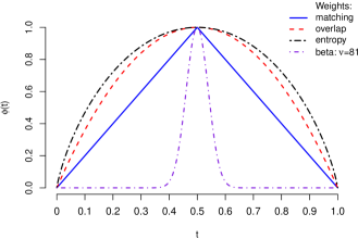
Figure 1: Examples of selection functions for equipoise

Figure 1 shows some of the selection functions for clinical equipoise. We scaled the selection functions such that the maximum $\displaystyle\phi(0.5)=1,$ for better visualization. It can shown that the beta distribution function $\displaystyle B_{1.7}(t)$ approximate the entropy function very well and that the beta functions $\displaystyle B_{\nu}(t)$, where $\displaystyle 3\leq\nu\leq 4$, can be good (and smooth!) approximations of the matching weight function. Clearly, the choice of $\displaystyle\nu$ has a direct impact on the treatment effect estimate. While $\displaystyle\nu>4$, seem to be an interesting choice to target patients with $\displaystyle t$ around 0.5, such an apparent advantage only helps reduce bias when the treatment effect is constant, but with less precision (especially when $\displaystyle\nu$ is large)—as shown by our simulation results. When the treatment effect is heterogeneous, it often leads to both biased and inefficient estimates as shown by our simulations. For instance, with $\displaystyle\nu=81$, $\displaystyle B_{\nu}(t)$ move faster to 0 as $\displaystyle t$ gets further away from 0.5. Most noticeable weights are concentrated among few observations with $\displaystyle t$ around 0.5 and these tends to drive the treatment effect estimate, which unfortunately will have a large variance.

More formally, we can show that $\displaystyle B_{1.8}(t)\leq\Omega(t)\leq B_{1.7}(t)$ and $\displaystyle B_{16}(t)\leq\Lambda(t)\leq B_{2.2}(t)$. This implies that, when the outcome is homoscedastic, the estimators based on the entropy and "matching" weight selection functions $\displaystyle-[t\ln(t)+(1-t)\ln(1-t)]$ and $\displaystyle\max(t,1-t)$ are always asymptotically less efficient that the estimator from the overlap weight selection function $\displaystyle t(1-t)$ since the latter is has the smallest asymptotic variance, under homoscedasticity, among all the selection functions $\displaystyle g$ (see Li et al., ⁵⁴ Corollary 1). In addition, from a practical standpoint, the entropy weights can still be extremely large or undefined whenever the propensity scores for some participants are near (or literally equal to) 0 and 1 while the imperative to smooth out the matching weight function around the maximum 1/2 can be a hindrance to its implementation , especially when dealing with multiple treatments.⁵⁰

While the selection functions for the ATE, ATT, and ATC are also special cases of beta functions, they are not (according to our definition and criteria (1)–(4)) good candidate functions to target the subpopulation of patients for whom there is clinical equipoise in our context. In addition, the indicator selection function $\displaystyle\mathds{1}({\{\alpha\leq t\leq 1-\alpha\}})$, $\displaystyle 0<\alpha<0.5$ of Crump et al., ²¹ the truncation selection function, and the trapezoidal function of Mao et al. ⁵³ defined as $\displaystyle\min\left\{1,K\!\min\{t,1-t\}\right\},$ for $\displaystyle K>1$ do not satisfy some of the above conditions.

Table 2 summarizes the list of selection functions that target the subpopulation of participants for whom there is equipoise we will consider for the remaining of this paper when we evaluate the equipoise treatment effect.

Table 2: Selection functions and weights for clinical equipoise

[] Weights Name $\displaystyle g(x)$ $\displaystyle w_{1}(x)$ $\displaystyle w_{0}(x)$ matching $\displaystyle u(x)$ $\displaystyle\min\left\{1,~{}{(1-e(x))}e(x)^{-1}\right\}$ $\displaystyle\min\left\{1,~{}{e(x)}{(1-e(x))^{-1}}\right\}$ beta $\displaystyle b_{\nu}(x)$ $\displaystyle e(x)^{\nu-2}(1-e(x))^{\nu-1}$ $\displaystyle e(x)^{\nu-1}(1-e(x))^{\nu-2}$ overlap $\displaystyle b_{2}(x)$ $\displaystyle 1-e(x)$ $\displaystyle e(x)$ entropy $\displaystyle\xi(x)$ $\displaystyle{\xi(x)}e(x)^{-1}$ $\displaystyle\xi(x)(1-e(x))^{-1}$

• $\displaystyle u(x)=\min\{e(x),1-e(x)\};$ $\displaystyle~{}b_{\nu}(x)=\left\{e(x)\left(1-e(x)\right)\right\}^{\nu-1}$, $\displaystyle\nu\geq 2$;

• $\displaystyle\xi(x)=-\left\{e(x)\ln(e(x))+\left(1-e(x)\right)\ln\left(1-e(x)\right)\right\}$.

4.3 A geometric interpretation

In the same vein as the importance sampling perspective, conditions (1)–(4) specify the subpopulation of patients we target by using the selection functions for equipoise. Let $\displaystyle\mathcal{S}_{1}(X)$ (resp. $\displaystyle\mathcal{S}_{0}(X)$) be the support of $\displaystyle X$ for the treatment (resp. control) group, i.e., the smallest closed set such as $\displaystyle P(X\in\mathcal{S}_{z}(X)|Z=z)=1$, for $\displaystyle z=0,1.$ Define the intersection $\displaystyle\mathcal{S}(X)=\mathcal{S}_{0}(X)\cap\mathcal{S}_{1}(X)$; every $\displaystyle x\in\mathcal{S}(X)$ belongs to the common support of the distribution of the covariates of participants in both groups. Therefore, $\displaystyle\mathcal{S}(X)$ represents the set of "matchable" participants. Ideally, to estimate ATE we expect to have $\displaystyle\mathcal{S}(X)=\mathcal{S}_{0}(X)=\mathcal{S}_{1}(X),$ which is not always guaranteed. When that is not realistic, we often fix our choice on the common support $\displaystyle\mathcal{S}(X)$ such that $\displaystyle\mathcal{S}(X)\subset\mathcal{S}_{z}(X),$ $\displaystyle z=0,1$ where the estimand $\displaystyle\tau_{g}$ is well defined for some $\displaystyle g$.

It is not always easy to specify $\displaystyle\mathcal{S}(X)$ in terms of the different baseline variables. Nevertheless, suppose that $\displaystyle\mathcal{U}(X)$ is the topological complement of the adherence of the set $\displaystyle\{X=x:g(x)=0\}$ where $\displaystyle g$ satisfies the conditions (1)–(4), then $\displaystyle\mathcal{U}(X)$ is the above common support. Naturally, $\displaystyle\mathcal{U}(X)$ includes $\displaystyle\mathcal{S}(X)$ since, by Bayes theorem,

$$\displaystyle f_{X|z}(x)=\left[p^{-1}e(x)\right]^{z}\left[(1-p)^{-1}(1-e(x))\right]^{z-1}f_{X}(x),~{}~{}\text{where}~{}~{}f_{X|z}(x)=P(X=x|Z=z)~{}~{}\text{and}~{}~{}p=P(Z=z).$$ (7)

As a consequence, the functions $\displaystyle g$ in Table 2 are good candidate functions to target the set of matchable participants. Hence, the above selection functions re-weights treatment and control groups as to potentially provide a large set of participants whose distributions $\displaystyle f_{X|z}(x)$ lead to adequate positivity. Therefore, as long as we can find a function $\displaystyle g$ and a related set $\displaystyle\mathcal{V}(X)$ such that $\displaystyle\mathcal{S}(X)\subset\mathcal{V}(X)\subset\mathcal{U}(X)$ and the influence of the points in $\displaystyle\mathcal{V}(X)\setminus\mathcal{S}(X)$ is minimal, then $\displaystyle\mathcal{V}(X)$ is a viable set to work with. We use the terms "influence" and "minimal" loosely and we will consider the subpopulations targeted via the matching weights function of Li and Greene ⁵², the overlap weights function of Li et al. ⁵⁴, and the above entropy function as good examples of such sets $\displaystyle\mathcal{V}(X)$, where we can estimate the treatment effect on a subpopulation of participants for whom positivity (and thus overlap of propensity scores) holds.

Using a geometric description, Shafer and Kang ¹⁷ demonstrated that patients in the treatment (resp. control) group are localized inside concentric ellipses with the highest concentration of treated (resp. control) individuals found around the center $\displaystyle E(X|Z=1)$ (resp. $\displaystyle E(X|Z=0)$). The further away we move from these center, the more sparse the number of observation becomes. Furthermore, the overall covariate average, $\displaystyle E(X)$, lies along the line segment that connects $\displaystyle E(X|Z=0)$ and $\displaystyle E(X|Z=1)$ with its position depending on the relative sizes of the two treatment groups. Since, $\displaystyle E(Y(z)|X)$, $\displaystyle z=0,1$ can be estimated most reliably for values of the covariates $\displaystyle X$ in the vicinity of $\displaystyle E(X|Z=z)$, better estimation the ATE depends on how well $\displaystyle E(Y(z)|X)$, $\displaystyle z=0,1$ can be predicted near the overall mean $\displaystyle E(X)$. Therefore, when $\displaystyle g(x)=1$ the two distributions $\displaystyle f_{X|z}(x)$ of the covariates are far apart in the sense that few individuals from both treatment groups are in the common region, the estimate of the ATE may require some extrapolation, ¹⁷ which may render the estimation of the ATE unstable and prone to bias. ^{61, 86} In Section 4.5, we demonstrate how and when, for a given function $\displaystyle g,$ the related estimand is closer to an ATT, an ATC or an ATE depending on the sample size of the treated participants and the variability of the propensity scores among the treatment groups.

4.4 Beta, matching, overlap, and Shannon’s entropy weights: close connections

4.4.1 The target population of the matching weights

The matching weights function was proposed by Li and Greene ⁵² as a so-called analogue to pair matching without replacement. However, it is not clear whether the estimand of interest is a deviation from the ATT or from the ATE. Although there are some similarities between the matching weight estimand and ATT (or ATC) estimand obtains via matching ²⁸, we demonstrate in this section that the matching weights by their nature do not solely target these estimand. Instead, they target an ATE-like estimand using the subpopulation of patients for whom there is equipoise.

The selection function for the matching weights of Li et al. ⁵² is the triangular distribution function $\displaystyle u(x)=\min\left(e(x),1-e(x)\right)$. This corresponds to the weights

$$\displaystyle w_{1}(x) \displaystyle=\displaystyle u(x)e(x)^{-1}=\min\left\{1,~{}e(x)^{-1}(1-e(x))\right\}~{}\text{and}~{}w_{0}(x)=\displaystyle u(x)(1-e(x))^{-1}=\min\{1,~{}e(x)(1-e(x))^{-1}\}$$ (8)

Using the above equations and the indicator $\displaystyle\kappa_{i}=\mathds{1}({\{\widehat{e}(x_{i})\leq 0.5\}})$, the estimator $\displaystyle\widehat{\tau}_{g}$ becomes

$$\displaystyle\widehat{\tau}_{g} \displaystyle=\displaystyle\sum_{i=1}^{N}\left[\displaystyle\frac{Z_{i}}{N_{\widehat{w}_{1}}}\min\left\{1,~{}\frac{(1-\widehat{e}(x_{i}))}{\widehat{e}(x_{i})}\right\}-\frac{(1-Z_{i})}{N_{\widehat{w}_{0}}}\min\left\{1,~{}\frac{\widehat{e}(x_{i})}{(1-\widehat{e}(x_{i}))}\right\}\right]Y_{i}$$

$$\displaystyle=\displaystyle\sum_{i=1}^{N}\left[{\kappa_{i}}\left(\frac{Z_{i}}{N_{\widehat{w}_{1}}}-\frac{\widehat{e}(x_{i})}{(1-\widehat{e}(x_{i}))}\frac{(1-Z_{i})}{N_{\widehat{w}_{0}}}\right)+(1-{\kappa_{i}})\left(\frac{(1-\widehat{e}(x_{i}))}{\widehat{e}(x_{i})}\frac{Z_{i}}{N_{\widehat{w}_{1}}}-\frac{(1-Z_{i})}{N_{\widehat{w}_{0}}}\right)\right]Y_{i}.$$ (9)

We can easily recognize the weights inside the square brackets in (4.4.1) . Whether a matching weight estimate differs from the one-to-one PS matching ATT estimate depends on how much treatment effects vary with the covariates X and on the range of values for the propensity scores $\displaystyle e_{i}(x).$ When $\displaystyle\widehat{e}_{i}(x)\leq 0.5$, the weights in (8) are proportional to the ATT weights whereas these weights are proportional to the ATC weights whenever all $\displaystyle\widehat{e}_{i}(x)>0.5$. Thus, the above $\displaystyle\widehat{\tau}_{g}$ is a combination of the estimator of the ATT and that of the ATC: it resembles an ATT estimator if all $\displaystyle e_{i}(x)\leq 0.5$ and an ATC estimator for $\displaystyle e_{i}(x)>0.5$. Namely, whenever $\displaystyle e_{i}(x)\leq 0.5$, matching weight algorithm assigns a weight equal to 1 to all treated participants, but weights control participants as to make them look like treated participants. However, when $\displaystyle e_{i}(x)>0.5$, the matching "weight" algorithm assigns to treated participants—who are usually overrepresented in this propensity score bracket—weights that make them look like those in the control group, just as we do when we estimate the ATC. Finally, when all $\displaystyle e_{i}(x)\approx 0.5$ (which is really unexpected in practice!), $\displaystyle\tau_{g}$ approximates simple mean outcome differences between the treatment groups.

In general, the estimator $\displaystyle\widehat{\tau}_{g}$ is a weighted average of the ATT and ATC. It does not target an ATT-like (or ATC-like) estimand per se as one-on-one propensity score matching does. Therefore, it does not correspond to an analog of an estimator obtained through propensity score "pair matching", as stated by Li and Greene.⁵²

So what does the estimand $\displaystyle\tau_{g}$ evaluate in this case and what does it represent? Based on equation (4.4.1), the matching weight algorithm revolves around group representation in terms of the corresponding propensity scores. Usually, treated patients are underrepresented in the lower half of the propensity score where $\displaystyle\{e_{i}(x)\leq 0.5\}$ and overrepresented when $\displaystyle\{e_{i}(x)>0.5\}$. Therefore, just like when we estimate the ATT, the matching weights (8) assign a weight equal to 1 to all treated participants in this lower range of the propensity scores, but weights control participants as to make them look like treated participants. Similarly, when the propensity scores is greater than 0.5, the matching weight algorithm assigns to treated participants, who are overrepresented in this propensity score bracket, weights that make treated participants to look like those in the control group and assign to control participants a weight equals to 1, just as we do when we estimate the ATC. In sum, the matching weights triage the participants by selecting only those for whom there is clinical equipoise and thus the underlying estimand is target the equipoise treatment effect, just like the overlap weights. Our illustrative example in Section 4.5.2 and the simulation results in Section 7 demonstrate these features of the matching weights.

4.4.2 Unexpected similarities

The aforementioned connections between the matching weights and overlap weights from Section 4.4.1 or among the selection functions of Section 4.2 are not the only unexpected similarities among their corresponding estimands. It is worth mentioning that when $\displaystyle e(x)\in[0.2,0.8],$ for all $\displaystyle x$, the OW estimator is close to the ATE, even when the treatment effect is heterogeneous since the selection function $\displaystyle g(x)=e(x)(1-e(x))\in$ $\displaystyle[0.16,0.25],$ i.e., nearly constant. Moreover, despite their apparent differences, connections between the overlap weight and the matching weight selection functions can be established. Several simulation studies and data applications have shown that matching weights and overlap weights yield similar point estimates for $\displaystyle\tau_{g}$ (see Li and Greene ⁵² and Mao et al. ⁵³). This can be explained by the inequality

$$\displaystyle\min\{t,1-t\}\leq 2t(1-t)\leq 1/8+\min\{t,1-t\},~{}~{}\text{for all }~{}t\in[0,1]$$ (10)

and by the fact that

$$\displaystyle t(1-t)=\displaystyle{\min\{t,1-t\}}\times{\max\{t,1-t\}},~{}~{}\text{for all}~{}t\in[0,1].$$ (11)

Therefore, the results at the end of Section 4.4.1 also applies to overlap weights, i.e., the OW estimator is a combination of the ATT and the ATC. Its estimate is close to ATT when most propensity scores $\displaystyle e(x)$ are less than 0.5 and close to the ATC if a large number of the propensity score $\displaystyle e(x)$ are greater than 0.5. This shed lights on the role of the matching weight estimand and, more generally, on all the estimand that based on selection function for whom there is clinical equipoise as we demonstrate in Section 4.5.

As we mentioned, the overlap weight function is part of the family of beta functions $\displaystyle g(x)=b_{\nu}(x)=[e(x)(1-e(x))]^{\nu-1},$ for which $\displaystyle\nu=2$. While some of these functions do not satisfy all the conditions (1)–(4) of section 4 when $\displaystyle\nu\leq 1$, those for which $\displaystyle\nu>1$ do. However, these functions are concave and strictly concave only when $\displaystyle 1<\nu\leq 2$. When $\displaystyle\nu$ gets larger than 2, these functions are no longer concave and not as roughly proportional to $\displaystyle e(x)(1-e(x))$ as we would expect, in order to obtain results that are similar to those from the overlap weight function.

Just as with the matching weight selection function, the maximum distance between the curves $\displaystyle t(1-t)$ and $\displaystyle-[t\ln(t)+(1-t)\ln(1-t)]$ is small and equal to $\displaystyle-1/4+\ln(2)\simeq 0.44.$ Case in point, using Taylor’s theorem with Cauchy remainder term, we can show that for $\displaystyle t\in[0,1],$

$$-\left[t\ln(t)+(1-t)\ln(1-t)\right]=t(1-t)\!\left(2+\frac{\rho-t}{2\rho^{2}}\right),~{}~{}\rho\in(0,1).$$ (12)

This implies that, in general, the point estimates from both the overlap weights and the entropy weights will also be very similar. In light of the results (11) and (12), we conclude that when the variances of the potential outcomes are homoscedastic, the overlap weight estimator is asymptotically more efficient than the matching weight, the entropy weight, and the beta weight estimators.⁵⁴ When there is heteroscedasticity, we do not guarantee such an efficiency, but expect the estimated variances from these estimators to be fairly similar or in favor of the overlap weights. This question is assessed in the simulation study in the context of finite samples.

That selection functions that are roughly proportional to $\displaystyle e(x)(1-e(x))$ will exhibit the same behavior as the overlap weight function is not fortuitous. In fact, the resemblance of the results from the matching, entropy, and overlap weights functions have been profusely demonstrated in classification and regression trees as well as in information theory where these functions are called, respectively, misclassification or Bayes error, cross-entropy or deviance, and Gini (impurity) index (see Breiman et al. ⁸⁸ or Hastie et al. ⁸⁹) The last two functions are the most commonly-used and, for practical reasons, the Gini index is the most preferred when dealing with categorical categorical variables. ⁸⁸ Finally, we can easily establish the relationship between the beta weights and the other three weights. For the matching weights, we just need to realize that the selection function $\displaystyle u(x)$ is also the so-called triangular distribution function; we can use the relationship between the beta and the triangular distributions to establish the connections between the beta and the matching weights. ⁹⁰

What separates the overlap weight function from the beta functions when $\displaystyle\nu>2$ is that the latter group of functions move faster to 0 as $\displaystyle e(x)$ moves away from the mode 0.5. Most observations will have very small normalized weights $\displaystyle w_{z}(x)/N_{wz}$ and the non-negligible weights will be concentrated on a very few partipants, with a spike around $\displaystyle e(x)=0.5$. This have two direct consequences in the estimation of the treatment effect using the beta weights when $\displaystyle\nu>2$: (1) the treatment effect is mostly driven by few observations with propensity scores around 0.5; (2) its estimated variance will tend to be larger compared to the variance from the other methods because of the presence of few observations with large weights (i.e., $\displaystyle e(x)\approx 0.5$) and a great number of observations with smaller weights, as shown in the illustrative example 4.5.2. While the selection function for $\displaystyle\nu>2$ seem to be a interesting choice when one needs to target participants with propensity scores around 0.5 and reduce bias, such an apparent advantage helps only in reducing bias when the treatment effect is constant. However, even then, it lacks precision and when the treatment effect is heterogeneous, it often leads to bias results.

4.5 Theoretical implications and an illustrative example

4.5.1 Theoretical implications

The inter-connections between the overlap weights, matching weights (10), (11) and entropy weights (12) along with the properties of the entropy weights lead to interesting theoretical implications and attractive features of selection functions $\displaystyle g(x)$ for clinical equipoise and the corresponding weights $\displaystyle w_{z}(x)$, $\displaystyle z=0,1$.

First, it is well-known that OW combine nicely two opposing-effect operations: minimizing the influence of extreme weights while improving the efficiency of the treatment effect estimator.^{20, 54} Therefore, as seen in practice, the overlap weight, matching weight, entropy weight and beta weight estimators achieve high degree of covariate balance for the variables included in the propensity score model, prevent loss of information, and provide efficient analysis results. Nevertheless, this important feature also means that cautious is warranted in selecting variables to include in the propensity score model. The goal is to adequately include all the confounding variables on the treatment-outcome relationship and prognostic variables (predictors of the outcome), using subject-matter knowledge of the study design and the outcome under study. Once such a judicious choice is made, these weights help us obviate the cyclical process of "propensity score tautology" where researchers repeatedly change the propensity score model specifications until they reach covariate balance.³⁴

Second, the above results reveal also an important fact: unless all the participants are such that $\displaystyle e_{i}(x)\leq 0.5$ (resp. $\displaystyle e_{i}(x)\geq 0.5$), the overlap weight, matching weight, and entropy weight estimators do not, in general, estimate the ATT (or ATC) per se. Because these estimators belong to the family of balancing weight estimators targeting the subpopulation of participants for whom there is equipoise, their estimates will be, in general, different from the ATE, ATT and ATC estimates whenever the treatment effect is heterogeneous.

As indicated in Section 4.3, $\displaystyle E(Y(z)|X)$, $\displaystyle z=0,1$ can be estimated most reliably for values of the covariates $\displaystyle X$ in the vicinities of $\displaystyle E(X|Z=z)$. Suppose $\displaystyle f({x})$ is the marginal distribution of the covariates $\displaystyle{X}$ and consider $\displaystyle f_{x|Z}(x|z)=P(X=x|Z=z)$ the density of the covariates $\displaystyle X$ in the treatment group $\displaystyle Z=z$. From (7), we have

$$\displaystyle\displaystyle{f_{X|z=1}(x)f_{X|z=0}(x)} \displaystyle=\frac{e(x)(1-e(x))}{p(1-p)}f_{X}(x),$$

which indicates that the contribution of each subpopulation defined by the covariates $\displaystyle X=x$ into $\displaystyle\widehat{\tau}_{g}$ mirrors directly the covariate joint density in the corresponding treatment $\displaystyle Z=z$ group. Whether $\displaystyle\tau_{g}$ is close to ATT (resp. ATC) can be anticipated by checking $\displaystyle p=P(Z=1)$ and $\displaystyle r(x)={\sigma_{1}^{2}(x)}\sigma_{0}(x)^{-2}$, where $\displaystyle\sigma_{z}^{2}(x)=\text{Var}[e_{i}(x)|Z=z],~{}z=0,1$. Indeed, the conditional density functions $\displaystyle f_{{\!\!e(x)|Z=z}}$ are related to the marginal density $\displaystyle f_{{\!\!e(x)}}$ via (see, for instance, Shaikh et al.⁹¹)

$$\displaystyle f_{{\!e(x)|Z=1}}(u) \displaystyle=\frac{u}{p}f_{{\!e(x)}}(u);~{}~{}f_{{\!e(x)|Z=0}}(u)=\frac{(1-u)}{(1-p)}f_{{}_{\!\!e(x)}}(u);~{}~{}\text{and thus}~{}~{}{f_{{\!e(x)|Z=1}}(u)}=\frac{(1-p)u}{p(1-u)}f_{{\!e(x)|Z=0}}(u)$$ (13)

which means the weights OW, MW, and EW assign to ATT (resp. ATC) decrease (resp. increase) in $\displaystyle p$ and $\displaystyle r(x)$. Thus, if $\displaystyle p$ or $\displaystyle r(x)$ is large, OW, MW, and EW are close to ATC. However, for small $\displaystyle r(x)$ and $\displaystyle p$, OW, MW, and EW approximate ATT. In particular, when $\displaystyle r(x)\approx 1,$ whether we obtain a result close to an ATT or an ATC depends solely on whether the prevalence $\displaystyle p$ is low or high. Using Rubin’s rule-of-thumb, we consider $\displaystyle r(x)\approx 1$ if its estimate $\displaystyle\widehat{r}(x)={\widehat{\sigma}_{1}^{2}(x)}\widehat{\sigma}_{0}(x)^{-2}$ satisfies $\displaystyle 0.5\leq\widehat{r}(x)\leq 2$; otherwise $\displaystyle r(x)$ is considered significantly different from 1.⁹²

Third, the simple case where $\displaystyle r(x)\approx 1$ sheds light on the difference between the weights assignment mechanisms of the overlap weight, matching, and entropy weight estimators compared to that of the IPW to estimate their respective estimator, with respect to the proportion $\displaystyle p$. Just as the overlap weight, matching, and entropy weight estimators are combinations of the ATT and ATC, so is the ATE estimator since $\displaystyle\text{ATE}=E[Y(1)-Y(0)]=pATT+(1-p)ATC$. However, how ATE weights ATT vs. ATT with respect to $\displaystyle p$ is in opposite direction of what the matching, overlap, or entropy weights estimators do. If the treatment effect is heterogeneous and $\displaystyle p$ is small, we can expect the ATE to be close to the ATC whereas the overlap weight, matching weight, and entropy weight estimands will be close to an ATT. On the other hand, if $\displaystyle p$ is relatively large, then ATT receives more weights with the ATE estimator while it is the ATC is weighted heavily with the overlap weight, matching weight, and entropy weight estimators. In short, when there are more treated than control participants overlap weight, matching weight, and entropy weight estimators give more weights to the ATC whereas the ATE estimator put more weights on the ATT instead, and vice-versa. How small (or large) should the proportion $\displaystyle p$ be for the difference between ATE estimated via IPW and the equipoise estimates to be noticeable? While an definitive answer to this question needs further investigations, in the case where $\displaystyle r(x)\approx 1$ we conjecture that difference will be noticeable whenever $\displaystyle p$ is outside of interval [0.2, 0.8] since $\displaystyle p(1-p)$ is fairly constant for $\displaystyle p\in$ [0.2, 0.8].

Of course, when the treatment effect is homogeneous and there is sufficient overlap in the underlying distribution of the covariates, we have $\displaystyle\text{ATE}=ATT=ATC$. In that case, the estimators obtained through the overlap weight, matching weight, or entropy weight framework or any matching algorithm will be asympotically similar. Furthermore, under small or moderate sample size, the overlap weight, matching weight, or entropy weight estimators will be less bias and more efficient than a pairwise PS matching estimator since the former estimation methods target and include a large sample of matchable participants and are more efficient.

4.5.2 Illustrative example

We consider a simple example using $\displaystyle\nu=11$ and $\displaystyle\nu=81$, $\displaystyle X=(X_{1},X_{2})$ with $\displaystyle X_{1}\sim N(2,2)$, $\displaystyle X_{2}\sim N(1,1)$. Let $\displaystyle Z\sim\text{Bernoulli}(e(X))$, where $\displaystyle e(X)=[1+\exp\left\{-(\alpha_{0}+\alpha_{1}X_{1}+\alpha_{2}X_{2})\right\}]^{-1}$, $\displaystyle Y(1)=2+X_{1}+X_{2}+2X_{1}^{2}+0.5X_{2}^{2}+\varepsilon_{1},$ with $\displaystyle\varepsilon_{1}\sim N(0,2)$, and $\displaystyle Y(0)=X_{1}+X_{2}+\varepsilon_{2},$ with $\displaystyle\varepsilon_{2}\sim N(0,1)$. We consider three different proportions $\displaystyle p=P(Z=1)$ of treatment participants, under a limited overlap of the distributions of the propensity scores, by carefully choosing values of $\displaystyle\alpha=(\alpha_{1},\alpha_{2},\alpha_{3})$ as follows: $\displaystyle\alpha=(-2.8,0.2,0.8)$, with $\displaystyle p\approx 20\%$ (Scenario A); $\displaystyle\alpha=(-1.6,0.45,0.6)$, with $\displaystyle p\approx 45\%-50\%$ (Scenario B); and $\displaystyle\alpha=(0.2,0.8,0.2)$, with $\displaystyle p\approx 80\%$ (Scenario C). The "true" estimands, provided in Table 3, are calculated using a "superpopulation" of size $\displaystyle 10^{7}$ participants, based on the true parameters coefficients, covariates, and models.

Table 3: True estimands

	Estimand
Scenario	ATE	ATT	ATC	OW	MW	EW	BW(11)	BW (81)
A	18.99	24.66	17.57	22.46	23.85	21.66	32.84	37.04
B	18.99	25.35	13.12	17.53	17.02	17.81	15.29	14.73
C	18.99	21.61	8.41	8.52	7.50	9.79	3.73	3.43

To investigate the above theoretical implications, we generated $\displaystyle M=1000$ data replicates to estimate the treatment effects under the 3 scenarios for $\displaystyle N=1000$.

Table 4: Estimated treatment effects

[] Scenario A Scenario B Scenario C ($\displaystyle p=0.20;~{}r(x)=1.74$) ($\displaystyle p=0.48;~{}r(x)=1.05$) ($\displaystyle p=0.80;~{}r(x)=0.4$) Est. ARB SE Est. ARB SE Est. ARB SE Crude 25.95 36.65 1.76 27.24 43.44 1.12 24.05 26.65 0.81 ATE 18.94 0.26 1.15 18.95 0.21 0.70 19.00 0.05 0.76 ATT 24.54 0.49 1.64 25.31 0.16 1.08 21.65 0.18 0.88 ATC 17.54 0.17 1.29 13.08 0.30 0.74 8.29 1.43 0.74 OW 22.36 0.44 1.20 17.49 0.23 0.67 8.47 0.57 0.54 MW 23.71 0.59 1.41 16.99 0.18 0.72 7.47 0.40 0.48 EW 21.57 0.42 1.10 17.77 0.22 0.65 9.73 0.61 0.58 BW(11) 32.69 0.46 3.98 15.32 0.20 1.10 3.78 1.34 0.40 BW(81) 36.99 0.13 7.83 14.80 0.48 1.50 3.50 2.04 0.71

• ARB: $\displaystyle 100\times$absolute relative bias

As opposed to the crude estimate, all the other methods (IPW for ATE and ATT, overlap weights, matching weights, entropy weights, and beta weights (for $\displaystyle\nu=11$ and $\displaystyle\nu=81$)) yield estimates that are close to their true values (see Table 4). Both scenarios A and B, correspond to $\displaystyle 0.5\leq\widehat{r}(x)\leq 2$. We see that when $\displaystyle p$ is only 0.20 (scenario A), the estimates of treatament effect for OW, MW, and EW are close the ATT estimated value and are all larger than the ATE estimate. When $\displaystyle p\approx 0.5$, as in scenario B, the true estimand and their estimated values for ATE, OW, MW, and EW are in the same ballpark, but apart from the ATT or ATC estimates. Finally, in scenario C, because $\displaystyle p\approx 0.8$ on average, the ATE estimate is near the estimate of the ATT, whereas the estimates of the treatment effect estimated OW, MW, and EW are close the ATC estimate of 8.29. Overall, this example makes the case for the above theoretical implicatons: (1) MW does not estimate the analogue to the one-on-one matching, but really a standalone estimand; (2) OW, MW, and EW are data-adaptive and naturally depend on the proportion of treated (or control) participants in the sample; (3) MW, OW, and EW are not some knock-off versions the ATE that we happen to estimate due to the lack of positivity. Rather, they are estimand that estimate the treatment effect on a specific subpopulation of participants,i.e., the subpopulation of participants for whom there is sufficient overlap (or clinical equipoise, whenever such a context is more appealing) as we have made clear in this paper.

5 Improving efficiency via augmentation

5.1 Brief overview

While the methods to estimate $\displaystyle\tau_{g}$ we have considered so far are based on estimating both the selection function $\displaystyle g$ and the propensity score $\displaystyle e(X),$ we can also use the selection function $\displaystyle g$ and outcome regression models as well as the combination of the selection function, propensity score, and regression models estimations. The latter is motivated by the need to improve efficiency, provided that we can estimate the propensity scores approximately very well. In addition, augmented estimators tend to be more robust to model misspecification.

Similar to the estimation the ATE, we leverage the augmentation framework of Robins et al. ⁹³ to combine the estimations of the selection function, the propensity score, and the regression models and improve the efficiency of the estimator $\displaystyle\widehat{\tau}_{g}.$

We consider the conditional mean models $\displaystyle m_{z}(X)=E(Y|Z=z,X)$, $\displaystyle z=0,~{}1.$ We have $\displaystyle E[g(X)m_{1}(X)]=E\left[g(X)Y(1)\right]$ and $\displaystyle E[g(X)m_{0}(X)]=E\left[g(X)Y(0)\right]$ (see Appendix A.1.2). Hence,

$$\displaystyle\frac{E[g(X)\left\{m_{1}(X)-m_{0}(X)\right\}]}{E[g(X)]}=\frac{E[g(X)\tau(X)]}{E[g(X)]}=\tau_{g},~{}~{}\text{where}~{}\tau(X)=E[Y(1)-Y(0)|X].$$

If we knew the true conditional expectations $\displaystyle m_{z}(X)$ and propensity scores $\displaystyle e(X)$, then the estimator

$$\displaystyle\displaystyle\left({\displaystyle\sum_{i=1}^{N}g(x_{i})}\right)^{-1}{\displaystyle\sum_{i=1}^{N}g(x_{i})\left\{m_{1}(x_{i})-m_{0}(x_{i})\right\}}$$ (14)

would have been a natural candidate for an unbiased and consistent estimator of the above $\displaystyle\tau_{g}.$ Unfortunately, we don’t usually know the true conditional expectation $\displaystyle m_{z}(X)$ or the true propensity score $\displaystyle e(X)$. Nevertheless, in addition to the propensity score model, we can also postulate a parametric model $\displaystyle m_{z}(X;\alpha_{z})$ for $\displaystyle E(Y|Z=z,X)$ and derive an estimator of $\displaystyle\tau_{g}$.

It is important to mention that the parametric models $\displaystyle m_{z}(X;\alpha_{z})$ are estimated separately and only on the subset of participants for which $\displaystyle Z=z$. Then, using the estimates $\displaystyle\widehat{\alpha}_{z}$ of the regression coefficients $\displaystyle\alpha_{z}$, $\displaystyle z=0,1,$ and the covariate values, we calculate for each participant in the sample (treated and control) the fitted values $\displaystyle\widehat{m}_{z}(x_{i})=m(x_{i};\widehat{\alpha}_{z})$ for $\displaystyle z=0$ and $\displaystyle z=1.$ ⁶⁷ Although not apparent, the conditional mean models $\displaystyle m_{z}(X)$ are well-defined only under the positivity assumption since $\displaystyle m_{z}(X)=\displaystyle\int yf_{Y|X,Z}(y|x,z)f(x)dydx$. Otherwise, whenever $\displaystyle e(x)=0$ or 1, we are conditioning on null event. ^{94, 17} Unfortunately, since estimating $\displaystyle m_{z}(X)$ does not require estimating propensity scores, the lack of adequate positivity or limited overlap may go unnoticed. Nevertheless, when there is a limited overlap in the distribution of covariates between the two treatment groups, the models $\displaystyle\widehat{m}_{z}(x_{i})=m_{z}(x_{i};\widehat{\alpha}_{z})$ extrapolate the relationship between the covariates $\displaystyle X$ and the outcome $\displaystyle Y$, from the overlap region of the distributions to the isolated regions of the distributions—where only observations from one treatment group is present or data are sparse.^{43, 95} However, the success of this extrapolation will depends strongly on how well we specify the model $\displaystyle m_{z}(x_{i};\widehat{\alpha}_{z})$, especially if there are nonlinear continuous variables.⁴³ Such an extrapolation in regions of no overlap, which may be different from the true relationship, can be perilous and drastically affect the efficiency of the estimator $\displaystyle\widehat{\tau}_{g}^{m}$. Moreover, it may lead to a biased and inefficient estimator of $\displaystyle\tau_{g}.$^{17, 18, 19}

5.2 Augmented weighted average treatment effects

For ATE, ATT, and ATC, we can write the corresponding selection function as $\displaystyle g(x)=a+be(x)$ with, respectively, $\displaystyle a=1,b=0$; $\displaystyle a=0,b=1$; and $\displaystyle a=1,b=-1$. The augmentation framework allows us, with $\displaystyle\widehat{w}_{z}(x)=(a+b\widehat{e}(x))\widehat{e}_{i}(x)^{-z}(1-\widehat{e}_{i}(x))^{z-1}$, $\displaystyle z=0,1$, to combine both estimators $\displaystyle\widehat{\tau}_{g}$ from (5) and $\displaystyle\widehat{m}_{z}(x_{i})$ into a more robust defined as

$$\displaystyle\widehat{\tau}_{g}^{DR} \displaystyle=\sum_{i=1}^{N}{Z_{i}\widehat{W}_{1}(x_{i})\left\{Y_{i}-\widehat{m}_{1}(x_{i})\right\}}-\sum_{i=1}^{N}{(1-Z_{i})\widehat{W}_{0}(x_{i})\left\{Y_{i}-\widehat{m}_{0}(x_{i})\right\}}+\sum_{i=1}^{N}\widehat{W}_{3}(x_{i})\left\{\widehat{m}_{1}(x_{i})-\widehat{m}_{0}(x_{i})\right\}$$ (15)

where $\displaystyle{\widehat{W}_{z}(x_{i})=\widehat{w}_{z}(x_{i})}\Big{/}{\displaystyle\sum_{i=1}^{N}\widehat{w}_{z}(x_{i})}$, $\displaystyle z=0,1$, and $\displaystyle{\widehat{W}_{3}(x_{i})=(a+bZ_{i})}\Big{/}{\displaystyle\sum_{i=1}^{N}(a+bZ_{i})}.$

Under the SUTVA, consistency, positivity, and unconfoundness assumptions, $\displaystyle\widehat{\tau}_{g}^{DR}$ is doubly robust, i.e., it is consistent if $\displaystyle\widehat{e}(X)$ or $\displaystyle\widehat{m}_{z}(X)$ is correctly specified, but not necessarily both. When the two models are correctly specified, $\displaystyle\widehat{\tau}_{g}^{DR}$ achieves asymptotic efficiency (see Tsiatis ⁹⁴ and Moodie et al. ⁹⁶).

Nevertheless, the estimator $\displaystyle\widehat{\tau}_{g}^{DR}$ has some drawbacks: (1) it is less efficient than $\displaystyle\widehat{\tau}_{g}$ if $\displaystyle e(X)$ is correctly specified, but $\displaystyle m_{z}(X)$ is misspecified or both the propensity score and regression models are not correctly specified; ^{67, 75} (2) its estimate is also sensitive to the lack of adequate positivity, especially if it is in addition to misspecified propensity score or regression models. The lack of adequate positivity affects directly estimation of the weights $\displaystyle\widehat{w}_{z}(x)$ and the extrapolation of $\displaystyle\widehat{m}_{z}(X)$ in the regions where the data are sparse. Let $\displaystyle\widetilde{e}(X)$ and $\displaystyle\widetilde{m}_{z}(X)$ denote, respectively, possibly misspecified propensity and regression models and consider $\displaystyle\widetilde{\tau}(X)=\widetilde{m}_{1}(X)-\widetilde{m}_{0}(X)$. Following Zhou et al., ⁴⁴ we show in Appendix A.2.2 that the asymptotic bias $\displaystyle\text{ABias}(\widehat{\tau}_{g}^{DR})$ of the estimator $\displaystyle\widehat{\tau}_{g}^{DR}$ is

$$\displaystyle E\left[\frac{(a+b\widetilde{e}(X))}{E\left[a+b\widetilde{e}(X)\right]}\widetilde{\tau}(X)-\frac{(a+be(X))}{E\left[a+be(X)\right]}\tau(X)\right]+E\left[\frac{e(X)(a+b\widetilde{e}(X))}{\widetilde{e}(X)}\right]^{-1}E\left[\frac{e(X)(a+b\widetilde{e}(X))}{\widetilde{e}(X)}\left\{m_{1}(X)-\widetilde{m}_{1}(X)\right\}\right]$$

$$\displaystyle-E\left[\frac{(1-e(X))(a+b\widetilde{e}(X))}{1-\widetilde{e}(X)}\right]^{-1}E\left[\frac{(1-e(X))(a+b\widetilde{e}(X))}{1-\widetilde{e}(X)}\left\{m_{0}(X)-\widetilde{m}_{0}(X)\right\}\right],~{}~{}\text{where}~{}~{}.$$ (16)

This clearly highlights the detrimental impact the combination of lack of adequate overlap and misspecification of the regression model can have on the final estimation of the treatment effect.

As we have argued, there would be little scientific basis to estimate the ATE in such a condition as the treatment effect would be based in part on extrapolation. Thus, the imperative to estimate the treatment effect on the subgroup of participants in the regions of overlap. For OW and MW, the current literature proposes the following augmented estimator ^{52, 53}

$$\displaystyle\widehat{\tau}_{g}^{aug} \displaystyle=\sum_{i=1}^{N}{Z_{i}\widehat{W}_{1}(x_{i})\left\{Y_{i}-\widehat{m}_{1}(x_{i})\right\}}-\sum_{i=1}^{N}{(1-Z_{i})\widehat{W}_{0}(x_{i})\left\{Y_{i}-\widehat{m}_{0}(x_{i})\right\}}+\sum_{i=1}^{N}\widehat{W}_{4}(x_{i})\left\{\widehat{m}_{1}(x_{i})-\widehat{m}_{0}(x_{i})\right\}$$ (17)

where $\displaystyle\widehat{w}_{z}(x_{i})=\widehat{g}(x_{i})\widehat{e}_{i}(x)^{-z}(1-\widehat{e}_{i}(x))^{z-1}$, $\displaystyle{\widehat{W}_{z}(x_{i})=\widehat{w}_{z}(x_{i})}\Big{/}{\displaystyle\sum_{i=1}^{N}\widehat{w}_{z}(x_{i})}$, , $\displaystyle z=0,1$, and $\displaystyle\widehat{W}_{4}(x_{i})=\widehat{g}(x_{i})\Big{/}\displaystyle\sum_{i=1}^{N}\widehat{g}(x_{i})$.

The estimator $\displaystyle\widehat{\tau}_{g}^{aug}$ is not affected by the lack of adequate positivity. When the propensity score and the regression models are correctly specified and $\displaystyle\widehat{\beta}$ and $\displaystyle\widehat{\alpha}_{z}$ are consistent, the estimator $\displaystyle\widehat{\tau}_{g}^{aug}$ is consistent and can achieve asymptotic efficiency, i.e., have the smallest asymptotic variance. Moreover, when the propensity score model is correctly specified and $\displaystyle\widehat{\beta}$ is consistent, the estimator $\displaystyle\widehat{\tau}_{g}^{aug}$ is also consistent. However, since the selection function $\displaystyle g(x)$ depends on $\displaystyle e(x)$, when the propensity score model $\displaystyle\widehat{e}(X)$ is misspecified, $\displaystyle\widehat{\tau}_{g}^{aug}$ is no longer consistent, even if the regression models $\displaystyle\widehat{m}_{z}(X)$ are correctly specified. Nevertheless, it tends to yield satisfactory results,⁵³ since it is commonly known that issues related to both propensity score misspecification and extrapolation of regression models matter most in area of limited covariate distrubitions overlap. ^{26, 13, 50, 18, 19, 97, 43} Its asymptotic bias $\displaystyle\text{ABias}(\widehat{\tau}_{g}^{aug})$, given by

$$\displaystyle\text{ABias}(\widehat{\tau}_{g}^{aug}) \displaystyle=E\left[\frac{\widetilde{g}(X)}{E\left[\widetilde{g}(X)\right]}\widetilde{\tau}(X)-\frac{g(X)}{E\left[g(X)\right]}\tau(X)\right]+E\left[\frac{e(X)\widetilde{g}(X)}{\widetilde{e}(X)}\right]^{-1}E\left[\frac{e(X)\widetilde{g}(X)}{\widetilde{e}(X)}\left\{m_{1}(X)-\widetilde{m}_{1}(X)\right\}\right]$$ (18)

$$\displaystyle-E\left[\frac{(1-e(X))\widetilde{g}(X)}{1-\widetilde{e}(X)}\right]^{-1}E\left[\frac{(1-e(X))\widetilde{g}(X)}{1-\widetilde{e}(X)}\left\{m_{0}(X)-\widetilde{m}_{0}(X)\right\}\right],$$

showcases how the selection function $\displaystyle\widetilde{g}(X)$ helps tremendously in the presence of observations with $\displaystyle\widetilde{e}(X)\approx 0$ or 1 since, in this case, $\displaystyle{e(X)\widetilde{g}(X)}/{\widetilde{e}(X)}$ and $\displaystyle{(1-e(X))\widetilde{g}(X)}/{(1-\widetilde{e}(X))}$ can be negligible.

Models misspecifications are more likely to lead a poor estimation of the regression parameters in these regions of limited overlap since there is a sparsity of treated (or control) participants and the performances of these model parameters are based on extrapolation of the misspecified models. ^{83, 67} The equation (18) indicates that the impact of the misspecifications on the asymptotic bias $\displaystyle\text{ABias}(\widehat{\tau}_{g}^{aug})$ is minor whenever $\displaystyle\widetilde{e}(X)\approx$ 0 or 1 since $\displaystyle\widetilde{g}(X)\left\{\widetilde{m}_{1}(X)-\widetilde{m}_{0}(X)\right\}$, $\displaystyle\frac{e(X)\widetilde{g}(X)}{\widetilde{e}(X)}\left\{m_{1}(X)-\widetilde{m}_{1}(X)\right\},$ and $\displaystyle\frac{(1-e(X))\widetilde{g}(X)}{1-\widetilde{e}(X)}\left\{m_{0}(X)-\widetilde{m}_{0}(X)\right\}$ are all negligible and do not contribute much to the asymptotic bias. Nevertheless, the impact of such misspecification in the asymptotic bias $\displaystyle\text{ABias}(\widehat{\tau}_{g}^{DR})$ of the augmented IPW estimator can be exacerbated by the presence of observations with $\displaystyle\widetilde{e}(X)\approx$ 0 or 1, as it can be seen in equation (5.2). For instance, for the ATE estimator with $\displaystyle a=1$ and $\displaystyle b=0$ the asymptotic bias (5.2) simplifies to

$$\displaystyle E\left[\left(E\left[\frac{e(X)}{\widetilde{e}(X)}\right]^{-1}\frac{e(X)}{\widetilde{e}(X)}-1\right)\left\{m_{1}(X)-\widetilde{m}_{1}(X)\right\}\right]-E\left[\left(E\left[\frac{1-e(X)}{1-\widetilde{e}(X)}\right]^{-1}\frac{1-e(X)}{1-\widetilde{e}(X)}-1\right)\left\{m_{0}(X)-\widetilde{m}_{0}(X)\right\}\right].$$

5.3 Why bother with augmentations if they are not doubly robust?

In light of the above remarks, it becomes clear that regardless of the function used to reach the target subpopulation of patients from whom there is clinical equipoise, their corresponding augmented estimators are not doubly robust. Nevertheless, augmentation provides some additional benefits. Clearly, when the propensity score model is correctly specified, it leads to a correct specification of the selection function $\displaystyle g(x).$ The augmentation yields an unbiased estimator, even when regression models are misspecified. Moreover, if the regression models are also correctly specified, it leads to an efficient estimator. Finally, in practice, since the weights for equipoise estimators smoothly (and gradually) downweight observations outside the overlap regions, augmented estimators tend to be more efficient, if our estimation of the propensity score model is correct or nearly correct.

It is well-known that regression models are effective when the covariate distributions between treated and control participants are similar. ^{17, 92} By smoothly removing observations outside of the overlap regions through OW, MW, or EW, the application regression models $\displaystyle{m}_{z}(X)$ to provide reliable and efficient treatment effects in the population of patients for whom there is clinical equipoise—provided some of the models are correctly specified, if not all. For instance, with misspecified propensity score model $\displaystyle\widetilde{e}(X))$ but correctly specified outcome models $\displaystyle{m}_{z}(X)$, the above asymptotic bias $\displaystyle\text{ABias}(\widehat{\tau}_{g}^{aug})$ in (18) simplifies to

$$\displaystyle E\left[\left(\frac{\widetilde{g}(X)}{E\left[\widetilde{g}(X)\right]}-\frac{g(X)}{E\left[g(X)\right]}\right)\tau(X)\right]$$

compared to the asymptotic bias $\displaystyle\text{ABias}(\widehat{\tau}_{g})$ of the Hájek-type estimator (5)

$$\displaystyle E\left[\left(E\left[\frac{e(X)\widetilde{g}(X)}{\widetilde{e}(X)}\right]^{-1}\frac{e(X)}{\widetilde{e}(X)}m_{1}(X)-E\left[\frac{(1-e(X))\widetilde{g}(X)}{1-\widetilde{e}(X)}\right]^{-1}\frac{1-e(X)}{1-\widetilde{e}(X)}m_{0}(X)\right)\widetilde{g}(X)\right]-E\left[\frac{g(X)\tau(X)}{E\left[g(X)\right]}\right].$$

Their difference

$$\displaystyle E\left[\left(E\left[\frac{e(X)\widetilde{g}(X)}{\widetilde{e}(X)}\right]^{-1}\frac{e(X)}{\widetilde{e}(X)}m_{1}(X)-E\left[\frac{(1-e(X))\widetilde{g}(X)}{1-\widetilde{e}(X)}\right]^{-1}\frac{1-e(X)}{1-\widetilde{e}(X)}m_{0}(X)-\frac{\tau(X)}{E\left[\widetilde{g}(X)\right]}\right)\widetilde{g}(X)\right].$$

indicates clearly the behavior of $\displaystyle\widehat{\tau}_{g}$ vis-à-vis $\displaystyle\widehat{\tau}_{g}^{aug}$. The biases are the same only when $\displaystyle\widetilde{e}(X)\approx e(X)$; in which case $\displaystyle\widetilde{g}(X)\approx g(X)$, i.e., the estimators $\displaystyle\widehat{\tau}_{g}$ and $\displaystyle\widehat{\tau}_{g}^{aug}$ $\displaystyle\longrightarrow\tau_{g}.$ Otherwise, if the distribution of the ratio $\displaystyle\widetilde{e}(X)/e(X)$ or $\displaystyle(1-\widetilde{e}(X))/(1-e(X))$ is skewed, this may drastically impact the overall difference between the two estimators. Therefore, combining OW, MW, and EW with regression models via augmentation can be advantageous.

Furthermore, whenever the regression models are correctly specified, $\displaystyle\widehat{\tau}_{g}^{aug}$ converges in distribution to $\displaystyle E\left[\widetilde{g}(X)(Y(1)-Y(0)\right]/E\left[\widetilde{g}(X)\right],$ for a misspecified propensity score model. Therefore, $\displaystyle\widehat{\tau}_{g}^{aug}$ still retains a causal interpretation provided the outcome regression models are correctly specified, even though it will be different from true estimate of $\displaystyle\tau_{g}$. It can be leverage to test for the (causal) "sharp" null hypothesis of no causal treatment effect. ²⁹

Admittedly, it is important to lay out the asymptotic properties of estimators as we have done so far. Nevertheless, it is equally important (if not more important) to investigate how different estimators behave under a finite sample size. In practice (where sample sizes are finite), combining the propensity score model and the outcome regression models to estimate augmented or doubly-robust estimators is better than dealing with either (5) or (14) alone. It is important to remember that the outcome models $\displaystyle\widehat{m}_{z}(X)$ play a preeminent role, compared to the propensity score model $\displaystyle\widehat{e}(X)$, in reducing bias and improving efficiency.

The estimators (17) improve over their counterparts in (5) by fine-tuning the estimators to substantially reduce bias when the propensity score is misspecified, but the regression models are correctly specified. Moreover, when both models are moderately misspecified, these estimators maintain a good performance compared to the IPW estimator—this matters the most, in practice, since it is not always easy to guarantee correctly specified propensity or regression models.⁶⁷ Our simulations studies indicate that these improvements compare more favorably that the augmented estimators (17).

In the advent of a misspecified propensity score model, it has been our experience that the augmentation framework lead to high efficiency as long as (1) a careful consideration is used in the estimation of both the outcome regression and propensity score models and (2) the covariate balance is reached with the estimated propensity scores. Such an advantage was also mentioned by Mao et al. ⁵³ as well as by Tao and Fu. ⁵⁷ This happens because weighting by $\displaystyle\widetilde{W}_{4}(X)$ in (17) still improves the performances of the augmented estimators for the overlap, "matching", and entropy weights by smoothly downweighting the influence of extreme weights at the tails of the distribution of the propensity scores, while the IPW doubly robust estimator may in fact unduly exacerbates the impact of these influential weights.

Insight into this surprising result can be found if we investigate the asymptotic behaviors of the estimators $\displaystyle\widehat{\tau}_{g}^{aug}.$ The asymptotic variance of $\displaystyle\widehat{\tau}_{g}^{aug}$ is the variance of its influence function $\displaystyle F_{\tau_{g}}$ (see Section A.2.1), i.e., for $\displaystyle\mathcal{W}=(X,Y(1),Y(0)),$

$$\displaystyle\allowdisplaybreaks\text{AVar}(\widehat{\tau}_{g}^{aug})= \displaystyle\,E_{\mathcal{W}}\left[\frac{g(X)^{2}}{E\left[g(X)\right]^{2}}\left\{\frac{\left(Y(1)-\tau_{g}^{1}\right)^{2}}{e(X)}+\frac{\left(Y(0)-\tau_{g}^{0}\right)^{2}}{1-e(X)}\right\}\right]$$ (19)

$$\displaystyle+\left[\frac{g(X)^{2}}{E\left[g(X)\right]^{2}}\left(\sqrt{\frac{1-e(X)}{e(X)}}\left(m_{1}(X)-\tau_{g}^{1}\right)+\sqrt{\frac{e(X)}{1-e(X)}}\left(m_{0}(X)-\tau_{g}^{0}\right)\right)^{2}\right].$$

Whenever $\displaystyle e(X)\approx$ 0 or 1, the contrast between the asymptotic variance of the IPW estimator (where $\displaystyle g(X)=1$) and those of the OW, MW, and EW estimators can be seen through the last equation (19). The four terms have a negligible impact on the asymptotic variance $\displaystyle\text{AVar}(\widehat{\tau}_{g}^{aug})$, since $\displaystyle\allowdisplaybreaks g(X)^{2}e(X)^{-1}\approx 0$, $\displaystyle g(X)^{2}(1-e(X))^{-1}\approx 0$, $\displaystyle g(X)^{2}\sqrt{(1-e(X))e(X)^{-1}}\approx 0$, and $\displaystyle g(X)^{2}\sqrt{e(X)(1-e(X))^{-1}}\approx 0$ in the regions of the propensity score spectrum where $\displaystyle e(X)\approx$ 0 or 1. Hence, the information leading to the estimation of $\displaystyle\tau_{g}^{aug}$ comes primarily from regions with sufficient overlap, i.e., where there is a good amount of common information on the treatment effect, carried out by both treatment groups.

However, for the IPW estimator, $\displaystyle\allowdisplaybreaks g(X)=1$ and thus the terms $\displaystyle\allowdisplaybreaks e(X)^{-1}$, $\displaystyle\allowdisplaybreaks(1-e(X))^{-1}$, $\displaystyle\allowdisplaybreaks\sqrt{(1-e(X))e(X)^{-1}}$, and $\displaystyle\allowdisplaybreaks\sqrt{e(X)(1-e(X))^{-1}}$ may take large values when $\displaystyle e(X)\approx$ 0 or 1, even if the true treatment effect is constant. Moreover, when $\displaystyle e(X)\approx$ 0 or 1, estimations of the regressions models $\displaystyle m_{z}(X),$ $\displaystyle z=0,1,$ are susceptible to extrapolation or model misspecification bias in these regions. Therefore, variance estimation for the IPW estimator depends on whether there is sufficient positivity. When the positivity assumption is satisfied, the estimator is consistent and has an asympotic normal distribution ⁹⁴. Otherwise, the central limit theorem may no longer apply since the variance of the the IPW estimator can be infinite and thus its asymptotic distribution may not be normally distributed.

6 Large sample properties

To estimate the treatment effect $\displaystyle\tau_{g}$, the propensity score or the outcome regression models are first estimated and then plugged into via the estimator (5) or (17). As outlined in the previous section, the uncertainty inherent to the estimation of the propensity score or regression models sips through the derivation of the different estimators. In estimating their variances, we should account for the fact that these models have been estimated. Following the approach of Lunceford and Davidian, ⁹⁸ we can derive the asymptotic distribution of the estimators $\displaystyle\widehat{\tau}_{g}$, $\displaystyle\widehat{\tau}_{g}^{aug}$, and $\displaystyle\widehat{\tau}_{g,\,\text{REF}}^{aug}$ and subsequently estimate their large-sample variances, using the standard M-estimation theory. This allows us to incorporate the uncertainty associated with the estimation of the propensity scores and derive an empirical sandwich variance estimator by replacing all expected values by their corresponding empirical averages (see Stefanski and Boos ⁹⁹ or Wooldridge ¹⁰⁰). In this section, we show how this can be done for $\displaystyle\widehat{\tau}_{g}$. The large-sample variances of $\displaystyle\widehat{\tau}_{g}^{aug}$ and $\displaystyle\widehat{\tau}_{\mathds{{}_{G}}}$ can be derived similarly. We give the detailed proofs for these estimators in the Appendix B.

To derive the large-sample variances, we can view the estimator of interest (i.e., $\displaystyle{\tau}_{g}$, $\displaystyle\tau_{g}^{aug}$, or $\displaystyle\tau_{g,\,\text{REF}}^{aug}$) as linear combination $\displaystyle\tau_{g}^{aug}=c^{\prime}\theta$ of the components of a vector $\displaystyle\theta$, for some $\displaystyle c=(c_{1},c_{2},\dots,c_{J})^{\prime}$. Using the solution $\displaystyle\widehat{\theta}$ to an estimating equation $\displaystyle\displaystyle\displaystyle\sum_{i=1}^{N}\Psi_{\theta}({X}_{i},Z_{i},Y_{i};\theta)=0$, with respect to $\displaystyle{\theta}$, we can determine the asymptotic behavior of the estimator of interest.

First, since $\displaystyle E[\Psi_{\theta}({X}_{i},Z_{i},Y_{i};\theta)]=0$, this implies that $\displaystyle\widehat{\theta}\longrightarrow\theta$ in probability, as $\displaystyle N\longrightarrow\infty$, under some regularity conditions. ⁹⁹ Therefore, by Slutsky’s theorem, the estimator will also be consistent. Moreover, $\displaystyle\sqrt{N}(\widehat{\theta}-{\theta})$ converges in distribution to the normal distribution $\displaystyle N({0},\Sigma({\theta}))$ where $\displaystyle\Sigma({\theta})=A(\theta)^{-1}B(\theta)\{A(\theta)^{\prime}\}^{-1}$. Therefore, a consistent estimator of $\displaystyle\Sigma({\theta})$ is then $\displaystyle\widehat{\Sigma}({\widehat{\theta}})=A_{N}(\widehat{\theta})^{-1}B_{N}(\widehat{\theta})\{A_{N}(\widehat{\theta})^{\prime}\}^{-1}$, where

$$\displaystyle A_{N}(\widehat{\theta}) \displaystyle=N^{-1}\displaystyle\sum_{i=1}^{N}\left[-\frac{\partial}{\partial{\theta^{\prime}}}\Psi_{\theta}({X}_{i},Z_{i},Y_{i})\right]_{\theta={\widehat{\theta}}}~{};~{}~{}A(\theta)=\lim_{N\rightarrow\infty}A_{N}(\widehat{\theta})$$

$$\displaystyle B_{N}(\widehat{\theta}) \displaystyle=N^{-1}\displaystyle\sum_{i=1}^{N}\Psi_{\theta}({X}_{i},Z_{i},Y_{i})\Psi_{\theta}({X}_{i},Z_{i},Y_{i})^{\prime}\big{|}_{\theta=\widehat{\theta}};~{}~{}B(\theta)=\lim_{N\rightarrow\infty}B_{N}(\widehat{\theta})$$

From $\displaystyle\widehat{\Sigma}({\widehat{\theta}})$, we derive an estimator of the variance of the estimator of interest as

$$\widehat{Var}({\widehat{\tau}_{g}})=N^{-1}\left[c^{\prime}\widehat{\Sigma}({\widehat{\theta}})c\right].$$ (20)

For example, for $\displaystyle\tau_{g}^{aug}=c^{\prime}\theta_{aug}=\tau_{1g}^{m}-\tau_{0g}^{m}+\mu_{1g}-\mu_{0g}$, we use the parameter vector $\displaystyle\theta=\theta_{aug}=(\beta^{\prime},\alpha_{1}^{\prime},\alpha_{0}^{\prime},\tau_{1g}^{m},\tau_{0g}^{m},\mu_{1g},\mu_{0g})^{\prime}$ and $\displaystyle c=(0,0,0,1,-1,1,-1)^{\prime}$. Thus, $\displaystyle\widehat{\theta}_{aug}=(\widehat{\beta}^{\prime},\widehat{\alpha}_{1}^{\prime},\widehat{\alpha}_{0}^{\prime},\widehat{\tau}_{1g}^{m},\widehat{\tau}_{0g}^{m},\widehat{\mu}_{1g},\widehat{\mu}_{0g})^{\prime}$, is then the solution to the estimating equation

$$\displaystyle\displaystyle\displaystyle\sum_{i=1}^{N}\Psi_{\theta_{aug}}({X}_{i},Z_{i},Y_{i}) \displaystyle=\displaystyle\sum_{i=1}^{N}\begin{bmatrix}\psi_{\beta}({X}_{i},Z_{i})\\ Z_{i}\psi_{\alpha_{1}}({X}_{i},Y_{i})\\ (1-Z_{i})\psi_{\alpha_{0}}({X}_{i},Y_{i})\\ g(X_{i})\{m_{1}(X_{i})-\tau_{1g}^{m}\}\\ g(X_{i})\{m_{0}(X_{i})-\tau_{0g}^{m}\}\\ Z_{i}w_{1}({X}_{i})(Y_{i}-m_{1}(X_{i})-\mu_{1g})\\ (1-Z_{i})w_{0}({X}_{i})(Y_{i}-m_{0}(X_{i})-\mu_{0g})\\ \end{bmatrix}=0$$

with respect to $\displaystyle\theta_{aug}=(\beta^{\prime},\alpha_{1}^{\prime},\alpha_{0}^{\prime},\tau_{1g}^{m},\tau_{0g}^{m},\mu_{1g},\mu_{0g})^{\prime},$ where $\displaystyle\widehat{\tau}_{zg}=\displaystyle\displaystyle\sum_{i=1}^{N}\widehat{W}_{4}(x_{i})\widehat{m}_{z}(x_{i})$ and $\displaystyle\widehat{\mu}_{zg}=\displaystyle\displaystyle\sum_{i=1}^{N}Z_{i}^{z}(1-Z_{i})^{1-z}\widehat{W}_{z}(x_{i})\{Y_{i}-\widehat{m}_{z}(x_{i})\}$, for $\displaystyle z=0,1.$ The functions $\displaystyle\psi_{\beta}({X}_{i},Z_{i}),$ and $\displaystyle\psi_{\alpha_{z}}({X}_{i},Z_{i},Y_{i})$ are, respectively, the score functions of the propensity score and regression models, which we use to solve for $\displaystyle\beta$ and $\displaystyle\alpha_{z}$.

We have shown in the Appendix B how to derive estimators of these sandwich variances for the estimators $\displaystyle{\tau}_{g}$, $\displaystyle\tau_{g}^{aug}$, and $\displaystyle\tau_{g,\,\text{REF}}^{aug}$ when the propensity score is estimated by a logistic regression model and the outcome models $\displaystyle m_{z}(x)$ are linear regression models. Among the regularity conditions (required to apply M-estimation theory), we need to have a smooth selection function $\displaystyle g$. Because the selection function $\displaystyle u(x)=\min\left(e(x),1-e(x)\right)$ for the "matching" weights is not differentiable at $\displaystyle e(x)=0.5$, Li et al. ⁵² use the smooth version $\displaystyle\widetilde{u}(x)$, which consists in replacing the portion of $\displaystyle u(x)$ around $\displaystyle e(x)=0.5$ by a cubic polynomial to satisfy the regularity conditions for the sandwich variance estimation.

Alternatively, when possible, the variance of $\displaystyle\widehat{\tau}_{g}$ can be estimated using a nonparametric bootstrap estimator. ⁸⁹ This is particularly important when the sample size $\displaystyle N$ is small or moderate, when one wants to estimate a confidence interval that does not rely on the asymptotic normality assumption, or when there is an inherent dependence between some of the observations such as in stratified, clustered, hierarchical or multilevel design. ¹⁰¹ In the latter case, strata or clusters of observations are resampled with repetition to preserve the correlation structure between dependent (or related) observations in each bootstrap sample.

Note, however, that the bootstrap technique can become extremely time-consuming when performing numerical simulations, analyzing a large healthcare claims database or dealing with large electronic health records. Furthermore, for the inverse probability weight (IPW) estimator, standard bootstrap methods are known to fail when there is lack of positivity as resampling with repetition can exacerbate issues related to propensity model convergence. ^{102, 18} Dealing with complex data structures in such a context and using standard bootstrap make inference more challenging, highly unreliable (possible high magnitude of data variations across bootstrap replicates), less optimal, and prone to errors.

7 Monte Carlo simulations

To assess the different estimators and evaluate the finite-sample performance, we considered a number of simulation studies based on a variety of settings via two specific data generating processes (DGPs). Our first DGP followed the design presented by Li and Greene ⁵² under both homogeneous and heterogeneous treatment effect to illustrate the role of overlap weights as well as the similarities, in point estimates, between the different estimates compared to those from the matching weights, the Shannon’s entropy weights and the beta weights. The chosen data generating process also helps highlight the issues inherent to the lack of adequate positivity associated with the inverse probability weighting estimators, the advantage of the equipoise estimators via augmentation, and the efficient of the overlap weights vis-à-vis all the other weights, especially the beta weights.

The second DGP is based on the design developed by Li et Li ⁵⁰ and focuses on the impact of the prevalence of treatment. The goal is to investigate the joint impact of random and structural violations of the positivity assumption while articulating the flexibility of overlap, matching, and Shannon’s entropy weights and the limits of beta weights. Throughout the simulations, we calculated the true estimands for IPW, OW, MW, EW, and BW ($\displaystyle\nu=11$ and $\displaystyle 81$) under heterogeneous treatment effect using "super-populations" of size $\displaystyle 10^{7}$ units, based on the true parameter coefficients, covariates, and models. For both DGPs, we run the simulations using 1000 replications for each scenario and we chose the sample size to be $\displaystyle N=2000$, to evaluate the finite-sample performance of the different estimators using the following measures: absolute relative bias percentage ARB, standard deviation (SD), standard error (SE), root mean squared error (RMSE) as well as the 95% coverage probability (CP).To be concise, we only present the first DGP and its results in this manuscript; the second DGP and the corresponding results are reported in the Appendix C.

7.1 First simulations

7.1.1 Data generating process (DGP)

We generated the covariates $\displaystyle\bm{X}=(X_{1},\dots,X_{4})$ and the treatment indicator $\displaystyle Z$ following the DGP of Li and Greene ⁵², with $\displaystyle X_{4}\sim Ber(0.5)$, $\displaystyle X_{3}\sim Ber(0.4+0.2X_{4})$,

$$\displaystyle\begin{pmatrix}X_{1}\\ X_{2}\end{pmatrix}\!\sim N\!\begin{bmatrix}\begin{pmatrix}X_{4}-X_{3}+0.5X_{3}X_{4}\\ -X_{4}+X_{3}+X_{3}X_{4}\end{pmatrix},\begin{pmatrix}2-X_{3}&0.25(1+X_{3})\\ 0.25(1+X_{3})&2-X_{3}\end{pmatrix}\end{bmatrix},$$

and $\displaystyle Z\sim Ber(e(\bm{X}))$, where $\displaystyle e(\bm{X})=[1+\exp\{-(\beta_{0}+\beta_{1}X_{1}+\dots+\beta_{4}X_{4})\}]^{-1}.$

We considered, respectively, $\displaystyle(\beta_{0},\beta_{1},\dots,$ $\displaystyle\beta_{4})=$ $\displaystyle\allowdisplaybreaks(-0.5,$ $\displaystyle 0.3,$ $\displaystyle 0.4,$ $\displaystyle 0.4,$ $\displaystyle 0.4)$, $\displaystyle(-1,$ $\displaystyle 0.6,$ $\displaystyle 0.8,$ $\displaystyle 0.8,$ $\displaystyle 0.8)$, and $\displaystyle(-1.5,$ $\displaystyle 0.9,$ $\displaystyle 1.2,$ $\displaystyle 1.2,$ $\displaystyle 1.2)$ for good, moderate, and poor overlap of PS distributions (with the average $\displaystyle p=$51.37%, 53.05%, and 52.77%, respectively), as shown in Figure 2.

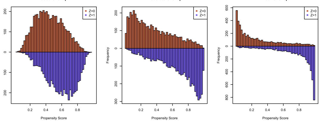
Figure 2: Distribution of propensity scores—with good (left), moderate (middle), and poor (right) overlap.

The first plot shows a good overlap of the distributions of the propensity scores between the two treatment groups, the middle graph indicates a case where the overlap is moderate while the last graph shows a poor overlap, i.e., there is a strong separation in estimated propensity scores between the treated and control participants. Finally, we generated the outcome $\displaystyle Y$ from the linear model $\displaystyle Y=0.5+\Delta Z+X_{1}+0.6X_{2}+2.2X_{3}+1.2X_{4}+\varepsilon$, where $\displaystyle\varepsilon\sim N(0,1)$ and $\displaystyle\Delta$ is the individual treatment effect. We choose, respectively, $\displaystyle\Delta=3$ (homogeneous treatment effect) and $\displaystyle-12e(\bm{X})^{2}+12e(\bm{X})+3$ (heterogeneous treatment effects), to compare the performance of the aforementioned methods.

We first assessed the Hájek estimators $\displaystyle\widehat{\tau}_{g}$ (5) of the weighted average treatment effect $\displaystyle\tau_{g}$ (1). Then, we evaluated the performance of the augmented estimators $\displaystyle\widehat{\tau}_{g}^{aug}$ when both the propensity score and regression models are correctly specified and when at least one of them is misspecified. We misspecified the propensity score or the outcome model by omitting the covariate $\displaystyle X_{1}$ from the original correct model.

Table 5: Treatment effect estimation (without augmentation).

		Homogeneous treatment effect							Heterogeneous treatment effect
Weight	Overlap	True	ARB	RMSE	SD	SE	CP		True	ARB	RMSE	SD	SE	CP
IPW	Good	3.00	0.07	6.54	6.54	6.39	0.94		5.57	0.02	7.08	7.08	7.04	0.95
OW	Good	3.00	0.05	4.72	4.72	4.83	0.95		5.65	0.04	4.90	4.90	5.06	0.95
MW	Good	3.00	0.05	4.86	4.86	5.00	0.95		5.70	0.06	5.07	5.07	5.14	0.94
EW	Good	3.00	0.05	4.80	4.80	4.89	0.94		5.63	0.04	5.00	4.99	5.18	0.95
BW(11)	Good	3.00	0.08	7.29	7.29	7.40	0.96		5.88	0.08	7.67	7.66	7.51	0.95
BW(81)	Good	3.00	0.00	10.80	10.81	12.40	0.98		5.98	0.14	11.49	11.47	12.41	0.97
IPW	Mod	3.00	0.05	21.53	21.54	18.08	0.88		4.94	0.10	24.78	24.79	20.99	0.87
OW	Mod	3.00	0.06	5.55	5.55	5.56	0.95		5.33	0.07	6.56	6.55	6.38	0.94
MW	Mod	3.00	0.10	5.73	5.72	5.76	0.96		5.44	0.04	6.46	6.46	6.35	0.95
EW	Mod	3.00	0.06	5.89	5.89	5.83	0.94		5.26	0.07	7.05	7.04	6.87	0.94
BW(11)	Mod	3.00	0.28	9.20	9.16	9.38	0.95		5.86	0.07	9.18	9.18	9.51	0.96
BW(81)	Mod	3.00	0.36	15.27	15.24	17.42	0.97		5.98	0.09	15.19	15.18	17.51	0.98
IPW	Poor	3.00	1.28	52.00	51.89	36.69	0.77		4.49	1.05	58.47	58.31	42.23	0.77
OW	Poor	3.00	0.07	6.23	6.23	6.35	0.95		5.18	0.03	7.40	7.41	7.64	0.96
MW	Poor	3.00	0.05	6.34	6.34	6.58	0.96		5.32	0.06	7.33	7.32	7.56	0.95
EW	Poor	3.00	0.08	6.73	6.73	6.77	0.95		5.07	0.01	8.05	8.05	8.38	0.96
BW(11)	Poor	3.00	0.07	10.30	10.31	11.21	0.97		5.86	0.17	10.96	10.92	11.39	0.96
BW(81)	Poor	3.00	0.05	18.15	18.16	22.01	0.97		5.98	0.14	18.45	18.44	21.93	0.98

• These results are based on 1000 repetitions of the simulated data. Mod: Moderate; BW($\displaystyle\nu$): BW with $\displaystyle\nu=11$ and $\displaystyle 81$; ARB: absolute relative bias$\displaystyle\times 100$;

• RMSE: root mean-squared error$\displaystyle\times 100$; SD:empirical standard deviation$\displaystyle\times 100$; SE: average estimated standard error$\displaystyle\times 100$; CP: 95% coverage probability.

7.1.2 Simulation results

The treatment effect estimation using the propensity score weighting methods under comparison are shown in Table 5, for the Hajek-type estimators (5). As expected, when the overlap of the distributions of the propensity scores is good, all estimators provide estimates with low bias and small standard errors. The coverage probability (CP) is between 0.94 and 0.96, except for BW(81) for which the CP is greater than or equal to 0.97. Nevertheless, BW(81) have a lower bias compared to BW (11). The differences among estimators are more noticeable instead in the variability of the estimates, with OW, MW, and EW being the most efficient (SE $\displaystyle\approx 5$), followed by IPW, BW(11), and finally BW(81), for which SE $\displaystyle\approx 12.40$.

Under moderate overlap, IPW, OW, MW and EW have mostly smaller biases compared to BW(11) and BW (11). OW, MW and EW have the smaller variability ($\displaystyle SE<6$) and adequate CPs, while BW (11) has SEs around 9 and CPs below or equal to 0.96 and BW(81) has SEs around 17.40 and CP $\displaystyle>96$. IPW has a lower ARB than BW(11) and BW (11) with a constant treatment, but not when the treatment is heterogeneous. Both BW(11) and BW (11) are more efficient than IPW. In addition, the CPs of IPW are below the 0.90. The above trend in the performance of the estimators remain under poor overlap where the ARB of IPW is more than 16 times higher than those of the other estimators and its CP is now equal to 0.77. The only exception is that BW(81) is less bias than BW(11). Unfortunately, the gain in bias for BW(81) does not make up the loss in efficiency, as seen throughout all the scenarios we considered since its SEs are almost twice has much than those from BW(11).

Overall, under moderate and poor overlap, IPW is the most sensitive estimator due to the lack of adequate positivity. The corresponding relative bias and standard error of IPW estimates increase rapidly and can be much higher than those of the other methods as lack of overlap worsens from moderate to poor. In contrast, the family of balancing weights that target clinical equipoise perform stably, even under poor overlap, yielding treatment effect estimates with small biases and variances. However, the selected BW estimators (using the beta function with a relatively large $\displaystyle\nu=11$ and $\displaystyle 81$) are shown to be less accurate and less efficient compared to OW, MW, and EW, which are special cases or approximations of the beta function with smaller $\displaystyle\nu$ $\displaystyle(1\leq\nu\leq 4)$. The higher the value of $\displaystyle\nu$ (i.e., far away from 4), the less efficient the BW($\displaystyle\nu$) estimator.

The results for OW, MW, and EW are fairly consistent across treatment effects and different level of lack of positivity. Compared to IPW, the gains in RMSE are often substantial. For instance, in moderate (resp. poor) overlap the RMSEs of OW, MW, and EW are about 3.7 (resp. 7) times lower than that of IPW, for both homogeneous and heterogeneous treatment effects. Oddly enough, even the worst case of beta weights (with $\displaystyle\nu=81$) was doing better in terms of RMSE than the IPW under moderate and poor overlap.

Table 6: Homogeneous treatment effect estimation (with and without model misspecification).

			Model misspecification
			None					PS model misspecified
Weight	Overlap	True	ARB	RMSE	SD	SE	CP	ARB	RMSE	SD	SE	CP
IPW	Good	3.00	0.05	5.00	5.00	4.95	0.96	0.05	4.93	4.93	4.90	0.96
OW	Good	3.00	0.04	4.83	4.83	4.83	0.95	0.05	4.83	4.83	4.83	0.95
MW	Good	3.00	0.04	4.86	4.86	4.89	0.95	0.04	4.83	4.83	4.88	0.95
EW	Good	3.00	0.05	4.84	4.84	4.83	0.95	0.05	4.84	4.84	4.83	0.95
BW(11)	Good	3.00	0.02	5.79	5.79	5.82	0.95	0.02	5.49	5.49	5.66	0.96
BW(81)	Good	3.00	0.03	8.99	9.00	9.12	0.95	0.09	8.47	8.47	8.75	0.95
IPW	Mod	3.00	0.01	7.24	7.25	6.93	0.94	0.02	6.41	6.42	6.18	0.95
OW	Mod	3.00	0.04	5.58	5.58	5.56	0.95	0.03	5.55	5.55	5.52	0.95
MW	Mod	3.00	0.03	5.65	5.65	5.66	0.95	0.03	5.61	5.61	5.61	0.96
EW	Mod	3.00	0.03	5.64	5.64	5.58	0.96	0.03	5.59	5.60	5.54	0.95
BW(11)	Mod	3.00	-0.01	7.80	7.81	7.77	0.95	0.00	7.33	7.33	7.37	0.95
BW(81)	Mod	3.00	-0.04	13.18	13.18	12.74	0.94	0.11	11.68	11.68	11.87	0.94
IPW	Poor	3.00	0.01	12.69	12.69	10.35	0.93	-0.01	8.25	8.25	8.02	0.96
OW	Poor	3.00	0.05	6.32	6.32	6.35	0.95	0.06	6.16	6.16	6.19	0.95
MW	Poor	3.00	0.03	6.43	6.44	6.48	0.96	0.06	6.25	6.25	6.29	0.95
EW	Poor	3.00	0.05	6.36	6.36	6.40	0.95	0.06	6.17	6.17	6.22	0.95
BW(11)	Poor	3.00	-0.04	9.32	9.32	9.42	0.95	0.06	8.57	8.57	8.64	0.95
BW(81)	Poor	3.00	-0.11	14.95	14.95	15.59	0.96	-0.01	13.82	13.83	13.97	0.95
			Outcome model misspecified					Both models misspecified
Weight	Overlap	True	ARB	RMSE	SD	SE	CP	ARB	RMSE	SD	SE	CP
IPW	Good	3.00	0.07	5.24	5.24	5.22	0.95	13.90	42.35	7.39	7.53	0.00
OW	Good	3.00	0.06	4.83	4.83	4.83	0.95	13.80	42.02	7.23	7.37	0.00
MW	Good	3.00	0.05	4.95	4.95	4.95	0.95	13.76	41.92	7.31	7.43	0.00
EW	Good	3.00	0.06	4.85	4.85	4.85	0.95	13.82	42.09	7.24	7.38	0.00
BW(11)	Good	3.00	0.03	6.93	6.93	6.81	0.95	13.60	41.71	8.60	8.61	0.00
BW(81)	Good	3.00	0.06	12.45	12.45	12.38	0.95	13.63	43.11	13.63	13.37	0.14
IPW	Mod	3.00	0.24	10.93	10.91	9.55	0.92	26.82	81.09	10.07	9.55	0.00
OW	Mod	3.00	0.05	5.59	5.59	5.56	0.95	25.97	78.35	8.42	8.11	0.00
MW	Mod	3.00	0.04	5.72	5.72	5.76	0.95	25.77	77.77	8.48	8.21	0.00
EW	Mod	3.00	0.07	5.75	5.75	5.65	0.95	26.11	78.80	8.51	8.17	0.00
BW(11)	Mod	3.00	-0.00	9.73	9.74	9.57	0.94	24.97	75.72	11.05	10.86	0.00
BW(81)	Mod	3.00	-0.09	18.05	18.06	17.37	0.94	24.77	76.45	17.99	17.74	0.02
IPW	Poor	3.00	1.04	22.84	22.64	16.44	0.83	38.62	116.70	14.09	12.66	0.00
OW	Poor	3.00	0.07	6.31	6.31	6.36	0.95	35.91	108.09	8.88	8.73	0.00
MW	Poor	3.00	0.07	6.53	6.53	6.60	0.95	35.45	106.73	8.95	8.83	0.00
EW	Poor	3.00	0.08	6.45	6.44	6.53	0.95	36.33	109.37	9.05	8.84	0.00
BW(11)	Poor	3.00	0.11	11.56	11.56	11.64	0.95	33.69	101.85	12.46	12.30	0.00
BW(81)	Poor	3.00	0.23	20.29	20.29	20.95	0.96	33.37	102.13	20.18	20.25	0.00

• These results are based on 1000 repetitions of the simulated data. Mod: Moderate; BW($\displaystyle\nu$): BW with $\displaystyle\nu=11$ and $\displaystyle 81$; ARB: absolute relative bias$\displaystyle\times 100$;

• RMSE: root mean-squared error$\displaystyle\times 100$; SD:empirical standard deviation$\displaystyle\times 100$; SE: average estimated standard error$\displaystyle\times 100$; CP: 95% coverage probability.

Table 7: Heterogeneous treatment effect (with and without model misspecification).

			Model misspecification
			None					PS model misspecified
Weight	Overlap	True	ARB	RMSE	SD	SE	CP	ARB	RMSE	SD	SE	CP
IPW	Good	5.57	0.03	5.42	5.42	5.45	0.95	0.60	6.20	5.23	5.30	0.91
OW	Good	5.65	0.02	5.02	5.02	5.10	0.96	0.08	5.06	5.04	5.12	0.95
MW	Good	5.70	0.00	5.00	5.01	5.10	0.96	-0.14	5.09	5.03	5.12	0.95
EW	Good	5.63	0.03	5.05	5.05	5.10	0.96	0.19	5.16	5.05	5.11	0.95
BW(11)	Good	5.88	-0.06	5.83	5.82	5.84	0.95	-0.88	7.80	5.81	5.75	0.85
BW(81)	Good	5.98	-0.10	8.90	8.89	9.12	0.95	-1.16	11.09	8.68	8.82	0.87
IPW	Mod	4.94	0.25	12.44	12.39	11.45	0.92	3.69	20.57	9.59	9.14	0.45
OW	Mod	5.33	0.07	6.73	6.72	6.66	0.95	0.55	7.40	6.80	6.71	0.92
MW	Mod	5.44	0.04	6.60	6.60	6.50	0.95	-0.07	6.74	6.73	6.60	0.95
EW	Mod	5.26	0.09	6.98	6.97	6.74	0.94	1.04	8.83	6.93	6.75	0.87
BW(11)	Mod	5.86	-0.08	8.20	8.19	7.83	0.94	-2.36	16.06	8.17	7.87	0.57
BW(81)	Mod	5.98	-0.14	13.38	13.36	12.75	0.93	-2.88	21.44	12.74	12.41	0.71
IPW	Poor	4.49	1.03	31.06	30.73	20.72	0.81	8.14	40.19	16.76	14.18	0.26
OW	Poor	5.18	0.09	8.36	8.36	8.07	0.94	0.66	8.86	8.17	7.90	0.92
MW	Poor	5.32	0.03	7.92	7.93	7.79	0.94	-0.43	8.24	7.91	7.75	0.93
EW	Poor	5.07	0.14	9.10	9.08	8.27	0.93	1.64	11.88	8.47	8.03	0.80
BW(11)	Poor	5.86	-0.20	9.62	9.56	9.49	0.94	-4.54	28.29	9.64	9.57	0.21
BW(81)	Poor	5.98	-0.33	16.42	16.30	15.60	0.94	-5.48	36.11	15.16	15.15	0.42
			Outcome model misspecified					Both models misspecified
Weight	Overlap	True	ARB	RMSE	SD	SE	CP	ARB	RMSE	SD	SE	CP
IPW	Good	5.57	0.03	5.80	5.80	5.81	0.95	7.68	43.44	7.63	7.81	0.00
OW	Good	5.65	0.03	5.00	5.00	5.09	0.96	7.02	40.34	7.40	7.58	0.00
MW	Good	5.70	0.01	5.06	5.07	5.14	0.96	6.72	39.05	7.48	7.60	0.00
EW	Good	5.63	0.03	5.04	5.04	5.10	0.95	7.16	41.01	7.41	7.59	0.00
BW(11)	Good	5.88	-0.05	6.88	6.87	6.78	0.95	5.70	34.72	8.93	8.66	0.04
BW(81)	Good	5.98	-0.09	12.07	12.06	12.12	0.95	5.31	34.70	14.02	13.35	0.33
IPW	Mod	4.94	0.36	16.03	15.94	13.91	0.90	17.57	87.54	11.75	11.25	0.00
OW	Mod	5.33	0.08	6.66	6.65	6.57	0.95	13.02	70.01	9.06	8.79	0.00
MW	Mod	5.44	0.05	6.57	6.57	6.49	0.94	12.07	66.27	9.01	8.70	0.00
EW	Mod	5.26	0.11	7.00	6.98	6.69	0.93	13.75	72.91	9.20	8.88	0.00
BW(11)	Mod	5.86	-0.07	9.57	9.56	9.23	0.94	8.59	51.65	11.32	10.79	0.01
BW(81)	Mod	5.98	-0.16	16.67	16.65	16.31	0.94	7.74	49.67	18.06	17.36	0.24
IPW	Poor	4.49	1.54	39.45	38.86	25.50	0.75	28.78	130.52	18.88	16.10	0.01
OW	Poor	5.18	0.09	8.19	8.18	7.91	0.94	17.29	90.21	9.84	9.56	0.00
MW	Poor	5.32	0.04	7.85	7.86	7.75	0.94	15.58	83.42	9.54	9.39	0.00
EW	Poor	5.07	0.14	8.98	8.95	8.16	0.93	18.83	96.10	10.28	9.78	0.00
BW(11)	Poor	5.86	-0.13	11.11	11.09	11.01	0.95	9.32	55.95	12.19	11.95	0.01
BW(81)	Poor	5.98	-0.19	19.56	19.54	19.22	0.94	8.01	51.69	19.47	19.40	0.31

• These results are based on 1000 repetitions of the simulated data. Mod: Moderate; BW($\displaystyle\nu$): BW with $\displaystyle\nu=11$ and $\displaystyle 81$; ARB: absolute relative bias$\displaystyle\times 100$;

• RMSE: root mean-squared error$\displaystyle\times 100$; SD:empirical standard deviation$\displaystyle\times 100$; SE: average estimated standard error$\displaystyle\times 100$; CP: 95% coverage probability.

For the augmented estimators $\displaystyle\widehat{\tau}_{g}^{aug}$, the results are given in in Tables 6 and 7. When at least one model is correctly specified and the overlap is good, augmentation tends to improve bias and efficiency, overall. For instance, under homogeneous treatment, there is a substantial reduction in standard errors for IPW, BW(11), and BW(81) compared to the case without augmentation. The OW, MW, and EW estimators are still the most efficient, while IPW is more efficient than BW(11) and BW(81) under good and moderate overlap. When the overlap is poor, IPW is only better than BW(81), but not BW(11). Compared to IPW, the gains in RMSE under homogeneous treatment effect are less substantial. For instance, in moderate (resp. poor) overlap the RMSEs of OW, MW, and EW are about 1.2 (resp. 1.63) times lower than that of IPW, when both models or the outcome model is correctly specified. There are about 1.7 (resp. 2.5) when the propensity model is correctly specified. When both models are misspecified, there is an excessive amount of bias for all the estimators and, judging by the their corresponding coverage probabilities, it is very difficult to pick the best performing estimators.

Under heterogeneous treatment effect, the trends are similar to those from the homogeneous treatment as expected, with OW, MW, and EW being the most efficient, IPW is more efficient than BW(11) and BW(81) only when the overlap is good. When the overlap is moderate or poor, IPW is more efficient than BW(81), but less efficient than BW(11). The gain in RMSE vis-á-vis IPW for OW, MW, and EW for moderate (resp. poor) overlap, under heterogeneous treatment effect, is about 1.8 (resp. 2.6) when both models are correctly specified, 1.4 (resp. 1.8) when the outcome models are correctly specified, and 2.1 (resp. 3.3) when the propensity score model is correctly specified. Again, the RMSE of IPW is worse than that of the BW(81), in bias and RMSE, when the overlap is poor. This again highlight the inability of IPW estimator to handle violations of the positivity assumption.

Overall, OW, MW, and EW are more efficient that IPW despite the fact that the latter is doubly-robust. Of the trio OW, MW, EW, the OW estimator has best RMSE in most the scenarios we considered under homogeneous treatment effect, while MW is the best under heterogeneous treatment effect. IPW is better than BW(81) almost everywhere, but not better than BW(11) in a good number of scenarios.

7.2 Second simulations

The second simulation study also consider three degrees of propensity score distributions overlap (poor, moderate and good), but focuses on the impact of the proportion of treated participants (i.e., prevalence of treatment) in the sample, as explained in the Appendix C, under both homogeneous and heterogeneous treatment effects. The results, summarized in Tables C.1.2 and C.1.3, indicate that the prevalence of treatment heightens the differences in bias and efficiency across the methods; the smaller the prevalence of treatment the higher the bias and the variance of the estimators. We see similar trend as in the first set of simulations, when we compare the different estimators, for a given prevalence of treatment and whether the treatment is homogeneous or not: OW, MW, and EW are the most efficient (with similar SEs) compared to IPW, BW(11) and BW(81). There is not a case where IPW has a small ARB and its RMSE was better than those from BW(11) and BW(81) only when the overlap was good. Otherwise, when the overlap was moderate or poor, both BW(11) and BW(81) have better RMSE. For instance, under constant treatment and median (resp. low) prevalence, the RMSE of BW(11) is equal to 15.25 (resp. 24.07), that of BW (81) equal to 24.79 (resp. 40.43) whereas IPW shows 55.46 (resp. 124.92). We observe a similar pattern under heterogeneous treatment effect. For more details, please, see Tables C.1.2 and C.1.3 in the Appendix.

8 Data illustrations

To illustrate the methods we have discussed, we present 2 examples with different levels of overlap in propensity scores between treatment groups. In the first example, we assess the effects of fish consumption on blood mercury level using data from the National Health and Nutrition Examination Survey (NHANES) 2013–2014 (see Zhao et al.¹⁰³). The data set can be obtained through the R package CrossScreening. In the second example, we evaluate the effects of children smoking on their pulmonary function using data from the Childhood Respiratory Disease Study (see Rosner ¹⁰⁴), which can be obtained through the R package covreg. For parsimony, we do not present the results from the beta selection function with $\displaystyle\nu=81$ as the simulation studies indicate that for such a high of $\displaystyle\nu$ the performance of the methods is poor in these two contexts.

8.1 Fish consumption and blood mercury level

The binary exposure $\displaystyle Z=1$ (high fish consumption) if the person had more than 12 servings of fish or shellfish in the previous month. The NHANES data consist 1107 adults with 234 (21%) of them had high fish consumption. The data include participants’ total blood mercury levels (in microgram per liter) as well as their age, sex, income (with missing values imputed by the median), the indicator of missing income, race, education, ever smoked, and number of cigarettes smoked last month. The outcome variable is defined as $\displaystyle\log_{2}$(total blood mercury level).

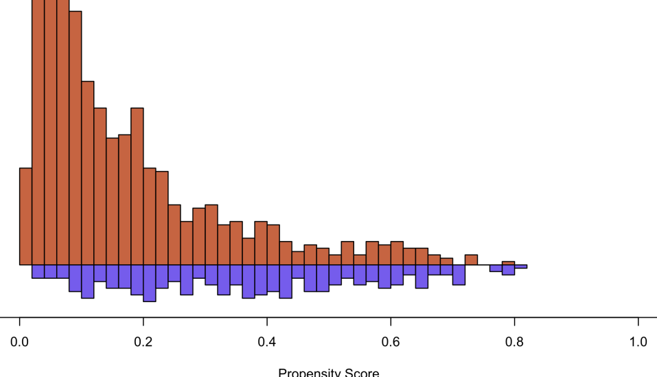
((a)) Propensity scores

	$\displaystyle N$	Min.	1st Qu.	Median	Mean	3rd Qu.	Max.
High fish consumption	234	0.02	0.23	0.37	0.36	0.49	0.77
Low fish consumption	873	0.004	0.05	0.12	0.17	0.24	0.75

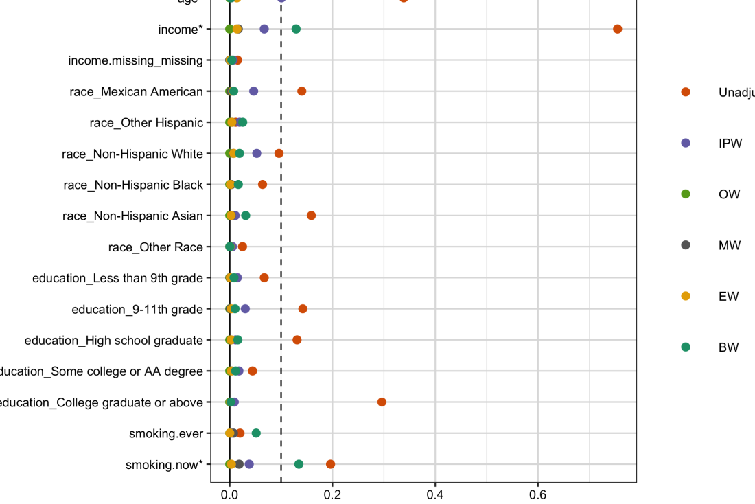
((b)) Covariate balance

Figure 3: NHANES data: Estimated propensity scores and covariate balance

((c)) Covariate balance in the unweighted sample and the sample weighted by inverse probability weights (IPW), overlap weights (OW), matching weights (MW), entropy weights (EW), and beta weights (BW).

The estimated propensity scores range from 0.004 to 0.77 with moderate level of overlap between the treated and control groups (Figure 3(a)). There is substantial imbalance in age, income, race, education, and number of cigarettes smoked, which can be mitigated by propensity score weighting (Figure 3(b)). The causal effects of fish consumption on blood mercury level, for the different weighting methods, are summarized in Table 8. While the point estimates of OW (1.99), MW (2.04), and EW (1.94) are similar, those of IPW (1.77) and BW (2.24) are slightly different. OW, MW, and EW are more efficient than IPW and BW in terms of standard error, effective sample size, and variance inflation. Augmentation improves the point estimation and the efficiency of IPW and BW estimators.

Table 8: NHANES data: Effect of fish consumption on $\displaystyle\log_{2}$(total blood mercury)

Estimator	Measure	IPW	OW	MW	EW	BW(11)
$\displaystyle\widehat{\tau}_{g}$	Estimate	1.77	1.99	2.04	1.94	2.24
	SE	0.13	0.10	0.10	0.09	0.18
$\displaystyle\widehat{\tau}_{g}^{aug}$	Estimate	1.80	2.00	2.04	1.95	2.22
(augmentation)	SE	0.10	0.10	0.09	0.10	0.10
	ESS	304.99	595.03	574.16	581.17	282.31
	VI	2.42	1.24	1.29	1.27	2.61

• SE: standard error; ESS: effective sample size; VI: variance inflation function

8.2 Smoking and force expiratory volume among children

The data consist of 654 children, aged 3–19, and include the children’s forced expiratory volume (FEV), age, sex, height, and smoking status. In total, 65 children (about 10%) were smokers, with the youngest smoker being 9 years old.

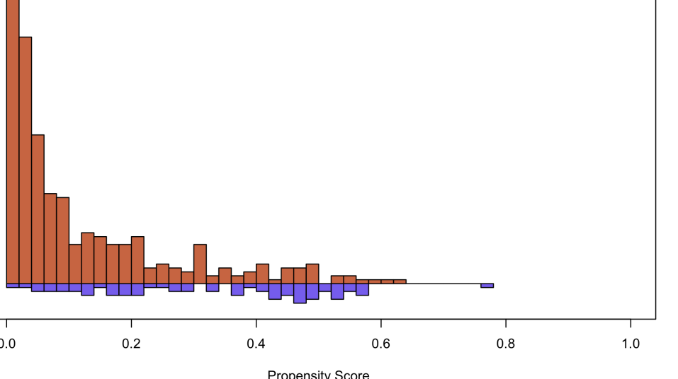
((a)) Propensity scores

	$\displaystyle N$	Min.	1st Qu.	Median	Mean	3rd Qu.	Max.
Smokers	65	0.0022	0.20	0.34	0.32	0.46	0.63
Non-smokers	374	0.0009	0.01	0.06	0.12	0.19	0.68

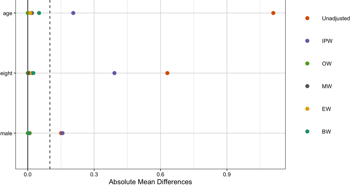
((b)) Covariate balance

Figure 4: FEV data: Estimated propensity scores and covariate balance.

((c)) Covariate balance in the unweighted sample and the sample weighted by inverse probability weights (IPW), overlap weights (OW), matching weights (MW), entropy weights (EW), and beta weights (BW).

We present the results for the subgroup of 439 children who are 9 years old or older. The estimated propensity scores range from 0.0009 to 0.68 with moderate to poor overlap between treatment groups (Figure 4(a)). Standard inverse probability weighting (IPW) fails to bring satisfactory balance in the three covariates (Figure 4(b)). Causal effect estimation for FEV data are summarized in Table 9. Due to the existence of extreme weights and poor overlap, the point estimates of IPW ($\displaystyle-0.58$) and BW ($\displaystyle-0.30$) are substantially different compares to those from OW ($\displaystyle-0.10$), MW ($\displaystyle-0.13$), and EW ($\displaystyle-0.12$) estimators, i.e., the class of weights targeting treatment equipoise. In addition, IPW and BW result in large standard error around the point estimates, 0.81 and 0.13 respectively compared to 0.07 for the equipoise estimators. Augmentation improves efficiency of IPW ($\displaystyle 0.07$) and BW ($\displaystyle 0.08$), and also pulls the point estimate of IPW (($\displaystyle-0.13$)) away from the non-parametric estimate ($\displaystyle-0.58$). The magnitude of the point estimate for BW decreased but remain high (more than twice the estimate of AW, MW, and EW). Nevertheless, the augmentation has drastically improve the variance estimation, going from 0.13 to 0.08. The point estimates and variances of the equipoise estimators for the augmented estimators barely budged from the non-augmented inference. Across both examples, OW and the class of weights targeting treatment equipoise maintain their efficiency compared to IPW and BW, regardless of the level of overlap.

Table 9: FEV data: Effect of smoking on FEV

[] Estimator Measure IPW OW MW EW BW(11) $\displaystyle\widehat{\tau}_{g}$ Estimate -0.58 -0.10 -0.13 -0.12 -0.30 SE 0.81 0.07 0.07 0.07 0.13 $\displaystyle\widehat{\tau}_{g}^{aug}$ Estimate -0.13 -0.11 -0.13 -0.11 -0.28 (augmented) SE 0.07 0.08 0.08 0.07 0.08 ESS 10.88 177.73 170.93 167.92 72.79 VI 20.37 1.25 1.30 1.32 3.04

• SE: standard error; ESS: effective sample size; VI: variance inflation function

9 Conclusion

This paper acknowledges that structural lack of positivity assumption is ubiquitous and should be handled appropriately. Whether lack of adequate positivity is expected or not, IPW with (or without) stabilized weights, trimming, or truncation can lead to bias and unstable results.^{43, 105} Furthermore, we have provided a number of examples where lack of adequate positivity is expected and sometimes welcomed. Our statistical analyses of these data structures cannot ignore lack of positivity, treat it as random, or even worse just use simple conventional methods. Handling structural lack of positivity often requires appropriate methods to yield accurate estimates and robust inference. These estimators have now risen in popularity, sparked lot of curiosity among a wide range of stakeholders, been implemented in many studies, and even have software packages made freely accessible for whomever want to use them. ^{80, 44, 106} In this paper, we have presented alternative methods that do not require the positivity assumption per se and handle treatment estimation appropriately, provided we focus our inference on the population of participants for whom there clinical equipoise. Therefore, the central role of this paper is to shed light on the role of the overlap weight estimator along with the three other related weighting estimators, i.e., the matching weight, the entropy weight, and the beta weight estimators.

Using mathematical derivations and large-sample properties, we have demonstrated that overlap weights, matching weights, Shannon’s entropy weights, and beta weights target indeed the same underlying estimand of interest: the equipoise average treatment effect, i.e., the treatment effect on the participants for whom there is clinical equipoise. The beta weights are a family of weights that target a wide range of estimands and that have, as special cases, the average treatment effect (ATE), the average treatment effect on the treated (ATT), the average treatment effect on the controls (ATC), and the average treatment effect of the overlap (ATO). The family can also approximate the matching weights (MW) and entropy weights (EW) very well. In this paper, we selected two specific beta weights, notably BW(11) and BW(81) to prove a point and answer questions we have been asked in our daily practices by clinical investigators: if $\displaystyle e(x)=0.5$ represent equipoise and since overlap weights focuses on participants whose propensity is around 0.5, could we make the windows where we select the participants in the neighborhood of 0.5? We have demonstrated that while such an inquiry is legitimate, there is a bias-variance trade-off we need to take into consideration. The choice of BW($\displaystyle\nu$) with $\displaystyle\nu$ far and far away from 4, achieves that desired neighborhood of $\displaystyle e(x)=0.5$, but often with biased and less efficient results.

The implementation of the methods presented in this paper is straightforward. What is challenging is the assessment of the underlying assumptions, which aid with correct estimation and inference of treatment effect. The use of the inverse probability weighting (IPW) methods (with truncation, trimming, or not) in the presence of lack of adequate positivity makes additional assumptions about the data that are not always elucidated or target an estimand, the ATE, when it is no longer valid since the assumptions are no longer valid—especially the positivity assumption.^{43, 44} The paucity of these key assessments of the assumptions creates lots of confusion, leads to controversy, and undermines the appreciation of innovative method, often deemed too complicated and fancy, with less motivation to adopt them. We have emphasized that a best practice to implementing the methods presented in this paper is to formulate the scientific questions of interest appropriately, define the goals of the study clearly, understand the structure of data pretty well, and elicit subjet-matter knowledge if necessary. In some cases, just drawing a directed acyclic graph (DAG) to decipher what variables to include in the propensity score or outcome regression models can help tremendously. More importantly, DAGs can aid to identify variables we should not include in our regression models (e.g., instrumental variables, mediators, and colliders).^{107, 108} As shown by the simulation study, variable selection and model specification are primordial to obtain reliable estimates of the treatment effect and reach sensible statistical inference.

While the methods presented in this paper focus on studies where a large number participants are eligible to either treatment, we recognize that the proportion of participants assigned to either treatment groups can influence directly the estimated treatment effect. Whether the proportion $\displaystyle p$ of participants assigned to the treatment group is small (resp. large) in the population, we know that the ATE is close to the average treatment effect on the control (ATC) (resp. the average treatment effect on the treated (ATT)) since $\displaystyle ATE=pATT+(1-p)ATC$. In this paper, we have demonstrated that the equipoise estimators would yield point estimates that are close the ATT (resp. ATC). We have illustrated such a phenomenon through simulation studies, which confirms the heuristic proof provided by Li et al.⁵⁴. Nevertheless, further investigations are warranted to assess the performance of different methods under finite sample size and maybe explain such a stark contrast in targeting specific (sub)population. Nevertheless, as we have demonstrated in this paper, deciding whether we need to estimate ATE or if it is even appropriate should not be limited to making sure that the SUTVA, uncounfoundness, and poistivity assumptions are satisfied, we need also to ensure that we have a balanced number of participants in both treatment groups. Otherwise, in addition to the issues inherent to propensity score methods at large, comparing different propensity score methods (matching, weighting, stratification) may not afford us to expect the results to be similar, especially when the underlying treatment effect we want to estimate is heterogeneous. We recommend the use of equipoise estimators as we gaining deeper understanding of their statistical properties—they are adaptive, data-sensible, flexible, and lead to efficient estimates. In addition, they always balance the distributions of the covariates included in the propensity score model.

We hope this paper will help those who would like to expand their statistical toolsets as the equipoise estimators (OW, MW, EW, and BW) offer an unprecedented opportunity to explore complex studies where lack of adequate positivity is not just by happenstance. Rather it is an integral part of the data underlying structure which should be acknowledged and handled appropriately. Whenever possible assessment of the assumptions and model specifications should always be conducted, but this cannot be done at the price of ignoring important tenets of causal inference: run observational studies that emulate randomized clinical trials and elicit experts’ opinion when necessary. Although we mainly focus on continuous outcomes, the methods presented in this paper can be extended to other types of outcomes and can easily be implemented using the PSweight R-package.¹⁰⁶

10 Acknowledgments

The authors are indebted to Yi Liu who read later versions of the manuscript and made valuable comments and suggestions, which helped improve the content of this paper.

Appendix A Technical details

A.1 The weighted estimator

A.1.1 Inverse weighted mean estimation

$$\displaystyle\allowdisplaybreaks E[Zw_{1}(X)] \displaystyle=E[Zg(X)e(X)^{-1}]=E[E\{Zg(X)e(X)^{-1}|X\}]$$

$$\displaystyle=E[g(X)e(X)^{-1}E(Z|X)]=E[g(X)]$$

Similarly, $\displaystyle E[(1-Z)w_{0}(X)]=E[(1-Z)g(X)(1-e(X))^{-1}]=E[E\{(1-Z)g(X)(1-e(X))^{-1}|X\}]=E[g(X)].$
Combining these results, lead to

$$\displaystyle E[Zw_{1}(X)+(1-Z)w_{0}(X)] \displaystyle=2E[g(X)]$$ (A.1.1)

Moreover,

$$\displaystyle\allowdisplaybreaks E[Zw_{1}(X)Y] \displaystyle=E[Zw_{1}(X)Y(1)]=E[Zg(X)e(X)^{-1}Y(1)]$$

$$\displaystyle=E\left[E\left\{Zg(X)e(X)^{-1}Y(1)\big{|}X,Y(1)\right\}\right]=E[g(X)e(X)^{-1}Y(1)E(Z|X,Y(1))]$$

$$\displaystyle=E[g(X)e(X)^{-1}Y(1)E(Z|X)]$$

$$\displaystyle=E[g(X)Y(1)]$$

$$\displaystyle E[(1-Z)w_{0}(X)Y] \displaystyle=E[(1-Z)w_{0}(X)Y(0)]=E[(1-Z)g(X)(1-e(X))^{-1}Y(0)]$$

$$\displaystyle=E\left[E\left\{(1-Z)g(X)(1-e(X))^{-1}Y(0)\big{|}X,Y(0)\right\}\right]$$

$$\displaystyle=E[g(X)(1-e(X))^{-1}Y(0)E(1-Z|X,Y(0))]=E[g(X)(1-e(X))^{-1}Y(0)E(1-Z|X)]$$

$$\displaystyle=E[g(X)Y(0)]$$

A.1.2 Estimation via regression models

By the SUTVA, $\displaystyle m_{z}(X)=E(Y|Z=z,X)=E[Y(z)|Z=z,X]$ while by the unconfoundness assumption $\displaystyle E(Y(z)|X)=E[Y(z)|Z=z,X],~{}z=0,1$. Therefore,

$$\displaystyle E[g(X)m_{1}(X)] \displaystyle=E\left[g(X)E(Y|Z=1,X)\right]=E\left[g(X)E(Y(1)|Z=1,X)\right]$$

$$\displaystyle=E\left[E(g(X)Y(1)|Z=1,X)\right]=E\left[E(g(X)Y(1)|X)\right]$$

$$\displaystyle=E\left[g(X)Y(1)\right].$$

Similarly,

$$\displaystyle E[g(X)m_{0}(X)] \displaystyle=E\left[g(X)E(Y|Z=0,X)\right]=E\left[g(X)E(Y(0)|Z=0,X)\right]$$

$$\displaystyle=E\left[E(g(X)Y(0)|Z=0,X)\right]=E\left[E(g(X)Y(0)|X)\right]$$

$$\displaystyle=E\left[g(X)Y(0)\right].$$

Thus,

$$\displaystyle\frac{E[g(X)\left\{m_{1}(X)-m_{0}(X)\right\}]}{E[g(X)]}=\frac{E\left[g(X)\left\{Y(1)-Y(0)\right\}\right]}{E[g(X)]}=\tau_{g}$$ (A.1.2)

Finally,

$$\displaystyle E\left[\left(Zw_{1}(X)+(1-Z)w_{0}(x)\right)m_{1}(X)\right] \displaystyle=E\left[\displaystyle\left\{Zg(X)e(X)^{-1}+(1-Z)g(X)(1-e(X))^{-1}\right\}m_{1}(X)\right]$$

$$\displaystyle=E\left[E\left\{\displaystyle Zg(X)e(X)^{-1}m_{1}(X)+\displaystyle(1-Z)g(X)(1-e(X))^{-1}m_{1}(X)|X\right\}\right]$$

$$\displaystyle=E\left[\displaystyle g(X)m_{1}(X)\left\{e(X)^{-1}E\left(Z|X\right)+\left(1-e(X)\right)^{-1}\displaystyle E\left((1-Z)|X\right)\right\}\right]$$

$$\displaystyle=E\left[\displaystyle g(X)m_{1}(X)\left\{e(X)^{-1}E\left(Z|X\right)+(1-e(X))^{-1}\displaystyle E\left((1-Z)|X\right)\right\}\right]$$

$$\displaystyle=2E\left[\displaystyle g(X)m_{1}(X)\right]$$ (A.1.3)

and

$$\displaystyle E\left[\left(Zw_{1}(X)+(1-Z)w_{0}(x)\right)m_{0}(X)\right] \displaystyle=E\left[\displaystyle\left\{Zg(X)e(X)^{-1}+(1-Z)g(X)(1-e(X))^{-1}\right\}m_{0}(X)\right]$$

$$\displaystyle=E\left[E\left\{\displaystyle Zg(X)e(X)^{-1}m_{0}(X)+\displaystyle(1-Z)g(X)(1-e(X))^{-1}m_{0}(X)|X\right\}\right]$$

$$\displaystyle=E\left[\displaystyle g(X)m_{0}(X)\left\{e(X)^{-1}E\left(Z|X\right)+\left(1-e(X)\right)^{-1}\displaystyle E\left((1-Z)|X\right)\right\}\right]$$

$$\displaystyle=E\left[\displaystyle g(X)m_{0}(X)\left\{e(X)^{-1}E\left(Z|X\right)+(1-e(X))^{-1}\displaystyle E\left((1-Z)|X\right)\right\}\right]$$

$$\displaystyle=2E\left[\displaystyle g(X)m_{0}(X)\right]$$ (A.1.4)

The results (A.1.1), (A.1.2), and (A.1.2) put together imply that

$$\displaystyle\frac{E[\left(Zw_{1}(X)+(1-Z)w_{0}(x)\right)\left\{m_{1}(X)-m_{0}(X)\right\}]}{E[\left(Zw_{1}(X)+(1-Z)w_{0}(x)\right)]}=\frac{E[g(X)\left\{m_{1}(X)-m_{0}(X)\right\}]}{E[g(X)]}=\frac{E[g(X)\tau(X)]}{E[g(X)]}=\tau_{g}$$ (A.1.5)

A.2 The augmented estimators

To demonstrate the results related to the augmentation of the estimator $\displaystyle\widehat{\tau}_{g}$, we consider that the SUTVA, consistency, positivity, and unconfoundness assumptions are satisfied.

Consider

$$\displaystyle\widehat{\tau}_{g}^{aug}=\displaystyle\sum_{i=1}^{N}Z_{i}\widehat{W}_{1}(x_{i})\left\{Y_{i}-\widehat{m}_{1}(x_{i})\right\}-\displaystyle\sum_{i=1}^{N}(1-Z_{i})\widehat{W}_{0}(x_{i})\left\{Y_{i}-\widehat{m}_{0}(x_{i})\right\}+\displaystyle\sum_{i=1}^{N}\widehat{g}(x_{i})\left\{\widehat{m}_{1}(x_{i})-\widehat{m}_{0}(x_{i})\right\}\big{/}\displaystyle\sum_{i=1}^{N}\widehat{g}(x_{i}).$$ (A.2.1)

Note that $\displaystyle\widehat{\tau}_{g}^{aug}$ is similar to the double robust estimator for normalized inverse probability weights given by Robins et al. ⁷⁵ (see the second version of their equation (1)).

If the selection function is affine, i.e., $\displaystyle g(x)=a+be(x)$, $\displaystyle a,b\in\mathbb{R},$ we use the following estimator instead

$$\displaystyle\widehat{\tau}_{g}^{DR} \displaystyle=\displaystyle\sum_{i=1}^{N}Z_{i}\widehat{W}_{1}(x_{i})\left\{Y_{i}-\widehat{m}_{1}(x_{i})\right\}-\displaystyle\sum_{i=1}^{N}(1-Z_{i})\widehat{W}_{0}(x_{i})\left\{Y_{i}-\widehat{m}_{0}(x_{i})\right\}+\displaystyle\sum_{i=1}^{N}\left(W_{3}(x_{i})\left\{\widehat{m}_{1}(x_{i})-\widehat{m}_{0}(x_{i})\right\}\right)$$ (A.2.2)

where $\displaystyle\allowdisplaybreaks\widehat{w}_{z}(x_{i})=(a+b\widehat{e}(x))\left[z_{i}\widehat{e}_{i}(x)^{-1}+(1-z_{i})(1-\widehat{e}_{i}(x))^{-1}\right]$ and $\displaystyle W_{3}(x_{i})={(a+bZ_{i})}\big{/}{\displaystyle\sum_{i=1}^{N}(a+bZ_{i})}.$

Notice that the ATE, ATT, and ATC correspond to the affine functions $\displaystyle g(x)=a+be(x)$ with, respectively, $\displaystyle b=0$; $\displaystyle a=0$; and $\displaystyle a=-b$. Their respective estimators via $\displaystyle\widehat{\tau}_{g}^{aug}$ are doubly robust and can achieve asymptotic efficiency (see Tsiatis ⁹⁴, Tan ¹⁰⁹, and Mercatanti and Li ¹¹⁰). We will demonstrate later that $\displaystyle\widehat{\tau}_{g}^{DR}$ is doubly robust.

A.2.1 General case

In general, how good of an estimator is $\displaystyle\widehat{\tau}_{g}^{aug}$ depends on how we specify the parametric models for $\displaystyle\widehat{e}(x),\widehat{g}(x)$ and $\displaystyle\widehat{m}_{z}(x)$, $\displaystyle z=0,1.$

First, suppose that the selection function $\displaystyle\widehat{g}(x)$ and the propensity score $\displaystyle\widehat{e}(x)$ are correctly specified, but the regression models $\displaystyle\widehat{m}_{z}(x)$ are misspecified, i.e., $\displaystyle\widehat{m}_{z}(X)\longrightarrow\widetilde{m}_{z}(X)\neq m_{z}(X)$. Using the results from Appendix A.1.1, we have

$$\displaystyle N^{-1}\displaystyle\sum_{i=1}^{N}Z_{i}\widehat{w}_{1}(x_{i}) \displaystyle\longrightarrow E(Zw_{1}(X))=E\left[g(X)\right]~{}~{}~{}\text{and}~{}~{}N^{-1}\displaystyle\sum_{i=1}^{N}(1-Z_{i})\widehat{w}_{0}(x_{i})\longrightarrow E((1-Z)w_{0}(X))=E\left[g(X)\right].$$ (A.2.3)

Also,

$$\displaystyle N^{-1}\displaystyle\sum_{i=1}^{N}Z_{i}\widehat{w}_{1}(x_{i})\left\{Y_{i}-\widehat{m}_{1}(x_{i})\right\}\longrightarrow E\left[g(X)\left\{Y(1)-\widetilde{m}_{1}(X)\right\}\right]$$ (A.2.4)

since $\displaystyle N^{-1}\displaystyle\sum_{i=1}^{N}Z_{i}\widehat{w}_{1}(x_{i})\left\{Y_{i}-\widehat{m}_{1}(x_{i})\right\}=N^{-1}\displaystyle\sum_{i=1}^{N}\frac{Z_{i}\widehat{g}(X_{i})}{\widehat{e}(X)}\left\{Y_{i}-\widehat{m}_{1}(x_{i})\right\}$ converges in probability to

$$\displaystyle E\left[\frac{Zg(X)}{e(X)}\left\{Y(1)-\widetilde{m}_{1}(X)\right\}\right] \displaystyle=E\left[E\left[\frac{Zg(X)}{e(X)}\left\{Y(1)-\widetilde{m}_{1}(X)\right\}\Big{|}Y(1),X\right]\right]=E\Bigg{[}g(X)\{Y(1)-\widetilde{m}_{1}(X)\}\frac{E(Z|Y(1),X)}{e(X)}\Bigg{]}$$

$$\displaystyle=E\left[g(X)\left\{Y(1)-\widetilde{m}_{1}(X)\right\}\frac{E(Z|X)}{e(X)}\right]=E\left[g(X)\left\{Y(1)-\widetilde{m}_{1}(X)\right\}\right],$$

since by the unconfoundness assumption, $\displaystyle E(Z|Y(1),X)=E(Z|X)=e(X).$

Similarly,

$$\displaystyle N^{-1}\displaystyle\sum_{i=1}^{N}(1-Z_{i})\widehat{w}_{0}(x_{i})\left\{Y_{i}-\widehat{m}_{0}(x_{i})\right\}\rightarrow E\left[g(X)\left\{Y(0)-\widetilde{m}_{0}(X)\right\}\right]$$ (A.2.5)

In addition,

$$\displaystyle N^{-1}\displaystyle\sum_{i=1}^{N}\widehat{g}(x_{i})\left\{\widehat{m}_{1}(x_{i})-\widehat{m}_{0}(x_{i})\right\}\longrightarrow \displaystyle E(g(X)\left\{\widetilde{m}_{1}(x_{i})-\widetilde{m}_{0}(x_{i})\right\})$$ (A.2.6)

We combine the equations (A.2.3)–(A.2.6) to conclude that $\displaystyle\widehat{\tau}_{g}^{aug}\longrightarrow\tau_{g}$, by the Slutsky’s Theorem ¹¹¹.

Therefore, whenever $\displaystyle g(X)$ is correctly specified, $\displaystyle\widehat{\tau}_{g}^{aug}\longrightarrow\tau_{g}$ if either the propensity score or the selection function are correctly specified. This proves that $\displaystyle\widehat{\tau}_{g}^{aug}$ is doubly robust, whenever $\displaystyle g(X)$ is correctly specified.

Furthermore, when the selection function, the propensity score model, and the regression models are all correctly specified, we can use the efficient influence function of the weighted average treatment effect to derive the asymptotic variance of $\displaystyle\widehat{\tau}_{g}^{aug}$ (as in Newey ¹¹²) given by $\displaystyle A\mathbb{V}(\widehat{\tau}_{g}^{aug})=\mathbb{V}(F_{\tau_{g}}(X,Z,Y))$ where $\displaystyle F_{\tau_{g}}(X,Z,Y)$ is the efficient influence function.
Using semiparametric theory ⁹⁴, the class of all influence functions of estimators of $\displaystyle\tau_{g}$ that are regular asymptotically linear (RAL) are given by $\displaystyle\displaystyle\frac{g(X)}{E\left[g(X)\right]}\left\{\bigg{[}\frac{Z(Y-\tau_{g}^{1})}{e(X)}\left.~{}-\frac{(1-Z)(Y-\tau_{g}^{0})}{1-e(X)}\right]+\left\{Z-e(X)\right\}h(X)\right\}$ for any arbitrary function $\displaystyle h(X).$ Therefore, following Theorem 13.1 (page 333) of Tsiatis ⁹⁴, there exist a unique efficient influence function $\displaystyle F_{\tau_{g}}(X,Z,Y)$, i.e., the one with the smallest variance among all the influences functions of RAL estimators of $\displaystyle\tau_{g}$ given by

$$\displaystyle F_{\tau_{g}}(X,Z,Y) \displaystyle=\displaystyle\frac{g(X)}{E\left[g(X)\right]}\bigg{[}\frac{Z(Y-\tau_{g}^{1})}{e(X)}-\frac{(1-Z)(Y-\tau_{g}^{0})}{1-e(X)}\bigg{]}-\displaystyle\frac{g(X)}{E\left[g(X)\right]}\Bigg{[}(Z-e(X))\left\{\frac{m_{1}(X)-\tau_{g}^{1}}{e(X)}+\frac{m_{0}(X)-\tau_{g}^{0}}{1-e(X)}\right\}\Bigg{]}$$

$$\displaystyle=\displaystyle\displaystyle\frac{g(X)}{E\left[g(X)\right]}\bigg{[}\frac{Z(Y-m_{1}(X))}{e(X)}-\frac{(1-Z)(Y-m_{0}(X))}{1-e(X)}+\left\{m_{1}(X)-m_{0}(X)\right\}-\tau_{g}\Bigg{]}.$$ (A.2.7)

We can calculate the asymptotic variance of $\displaystyle\widehat{\tau}_{g}^{aug}$ using the law of iterative variance, conditional with respect to $\displaystyle\mathcal{W}=(X,Y(1),Y(0))$ as $\displaystyle\text{AVar}(\widehat{\tau}_{g}^{aug})=Var_{\mathcal{W}}\left(E(F_{\tau_{g}}(X,Z,Y)|\mathcal{W})\right)+E_{\mathcal{W}}\left(Var(F_{\tau_{g}}(X,Z,Y)|\mathcal{W})\right),$ which is equal to

$$\displaystyle E_{\mathcal{W}}\left(\frac{g(X)^{2}}{\left(E\left[g(X)\right]\right)^{2}}\left\{{\frac{\left(Y(1)-\tau_{g}^{1}\right)^{2}}{e(X)}}+{\frac{\left(Y(0)-\tau_{g}^{0}\right)^{2}}{1-e(X)}}\right\}\right)$$

$$\displaystyle-E_{\mathcal{W}}\left[\left(\frac{g(X)}{E\left[g(X)\right]}\left\{\sqrt{\frac{1-e(X)}{e(X)}}\left(m_{1}(X)-\tau_{g}^{1}\right)+\sqrt{\frac{e(X)}{1-e(X)}}\left(m_{0}(X)-\tau_{g}^{0}\right)\right\}\right)^{2}\right].$$

It achieves the minimum variance when the regression models are correctly specified. However, if the selection function depends on the propensity score, it is crucial to have it correctly specified. Unless the selection function $\displaystyle g$ is an affine function of the propensity score, i.e., it is of the form $\displaystyle g(x)=a+be(x)$, $\displaystyle a,b\in\mathbb{R}$ (see A.2.3 ). Otherwise, whenever the propensity score is misspecified, i.e., $\displaystyle\widehat{e}(X)\longrightarrow\widetilde{e}(X)\neq e(x)=P(Z=1|X)$, the selection function is also misspecified, i.e., $\displaystyle\widehat{g}(X)\longrightarrow\widetilde{g}(X)\neq g(X)$. Therefore, $\displaystyle\widehat{\tau}_{g}^{aug}$ does not converges to $\displaystyle\tau_{g}$, even if the conditional regression models $\displaystyle\widehat{m}_{z}(X)$ are correctly specified.

A.2.2 Bias under model misspecifications

Suppose that $\displaystyle g(x)$ is not an affine function of $\displaystyle e(x)$ and that $\displaystyle\widehat{e}(X)\longrightarrow\widetilde{e}(X)$, possibly different from the true propensity score $\displaystyle e(X)=P(Z=1|X)$ and $\displaystyle\widehat{m}_{z}(X)\longrightarrow\widetilde{m}_{z}(X)$ and possibly different from $\displaystyle m_{z}(X)$. By the law of large numbers, $\displaystyle N^{-1}\displaystyle\sum_{i=1}^{N}Z_{i}\widehat{w}_{1}(x_{i})\left\{Y_{i}-\widehat{m}_{1}(x_{i})\right\}$ converges to $\displaystyle E\left[\frac{Z\widetilde{g}(X)}{\widetilde{e}(X)}\left\{Y(1)-\widetilde{m}_{1}(X)\right\}\right]=E\left[E\left[\frac{Z\widetilde{g}(X)}{\widetilde{e}(X)}\left\{Y(1)-\widetilde{m}_{1}(X)\right\}\Big{|}X\right]\right]$.

Thus, $\displaystyle N^{-1}\displaystyle\sum_{i=1}^{N}Z_{i}\widehat{w}_{1}(x_{i})\left\{Y_{i}-\widehat{m}_{1}(x_{i})\right\}\longrightarrow E\left[\frac{e(X)\widetilde{g}(X)}{\widetilde{e}(X)}\left\{m_{1}(X)-\widetilde{m}_{1}(X)\right\}\right]$ by the SUTVA and the unconfoundness assumption. Similarly, $\displaystyle N^{-1}\displaystyle\sum_{i=1}^{N}(1-Z_{i})\widehat{w}_{0}(x_{i})\left\{Y_{i}-\widehat{m}_{0}(x_{i})\right\}\longrightarrow E\left[\frac{(1-e(X))\widetilde{g}(X)}{1-\widetilde{e}(X)}\left\{m_{0}(X)-\widetilde{m}_{0}(X)\right\}\right].$

Finally, by the law of large numbers, we also have the following results:

$$\displaystyle N^{-1}\displaystyle\sum_{i=1}^{N}\widehat{g}(x_{i})\longrightarrow E\left[\widetilde{g}(X)\right];~{}~{}N^{-1}\displaystyle\sum_{i=1}^{N}Z_{i}\widehat{w}_{1}(x_{i})\longrightarrow E\left[Z\frac{\widetilde{g}(X)}{\widetilde{e}(X)}\right]=E\left[\frac{e(X)\widetilde{g}(X)}{\widetilde{e}(X)}\right];$$

$$\displaystyle N^{-1}\displaystyle\sum_{i=1}^{N}(1-Z_{i})\widehat{w}_{0}(x_{i})\longrightarrow E\left[(1-Z)\frac{\widetilde{g}(X)}{1-\widetilde{e}(X)}\right]=E\left[\frac{(1-e(X))\widetilde{g}(X)}{1-\widetilde{e}(X)}\right];$$

$$\displaystyle N^{-1}\displaystyle\sum_{i=1}^{N}\widehat{g}(x_{i})\left\{\widehat{m}_{1}(x_{i})-\widehat{m}_{0}(x_{i})\right\}\longrightarrow E(\widetilde{g}(X)\left\{\widetilde{m}_{1}(X)-\widetilde{m}_{0}(X)\right\})=E(\widetilde{g}(X)\widetilde{\tau}(X)),~{}~{}\text{with}~{}~{}\widetilde{\tau}(X)=E(\widetilde{g}(X)\left\{\widetilde{m}_{1}(X)-\widetilde{m}_{0}(X)\right\}).$$

Therefore, putting all together, we have

$$\displaystyle\widehat{\tau}_{g}^{aug}-\tau_{g} \displaystyle\longrightarrow E\left[\frac{\widetilde{g}(X)}{E\left[\widetilde{g}(X)\right]}\widetilde{\tau}(X)-\frac{g(X)}{E\left[g(X)\right]}\tau(X)\right]+E\left[\frac{e(X)\widetilde{g}(X)}{\widetilde{e}(X)}\right]^{-1}E\left[\frac{e(X)\widetilde{g}(X)}{\widetilde{e}(X)}\left\{m_{1}(X)-\widetilde{m}_{1}(X)\right\}\right]$$ (A.2.8)

$$\displaystyle-E\left[\frac{(1-e(X))\widetilde{g}(X)}{1-\widetilde{e}(X)}\right]^{-1}E\left[\frac{(1-e(X))\widetilde{g}(X)}{1-\widetilde{e}(X)}\left\{m_{0}(X)-\widetilde{m}_{0}(X)\right\}\right],~{}~{}\text{with}~{}~{}\tau_{g}=E\left[\frac{g(X)}{E\left[g(X)\right]}\tau(X)\right],$$

where $\displaystyle\widetilde{\tau}(X)=\widetilde{m}_{1}(X)-\widetilde{m}_{0}(X)$ and $\displaystyle\tau(X)=E[Y(1)-Y(0)|X]=m_{1}(X)-m_{0}(X).$

A.2.3 Special cases: affine selection functions

When the selection function $\displaystyle g$ is an affine function of the propensity score, i.e., $\displaystyle g(x)=a+be(x)$, $\displaystyle a,b\in\mathbb{R},$ however, we can re-define the augmentation au $\displaystyle\widehat{\tau}_{g}$ to obtain a doubly robust estimator. To do this, first notice that the sample average $\displaystyle N^{-1}\displaystyle\sum_{i=1}^{N}(a+bZ_{i})$ converges in probability to $\displaystyle E[(a+bZ)]=a+bE[E(Z|X)]=E[g(X)].$ Similarly, for any function $\displaystyle\zeta(.)$, the average $\displaystyle N^{-1}\displaystyle\sum_{i=1}^{N}(a+bZ_{i})\zeta(X_{i})$ also converges in probability to $\displaystyle E[(a+bZ)\zeta(X)]=a+bE[\zeta(X)E(Z|X)]=E[g(X)\zeta(X)].$

Thus, we can replace $\displaystyle\widehat{g}(x)=a+b\widehat{e}(x)$ in the first term of $\displaystyle\tau_{g}^{aug}$ by $\displaystyle a+bZ$ to obtain, for $\displaystyle a,b\in\mathbb{R}$,

$$\displaystyle\widehat{\tau}_{g}^{DR} \displaystyle=\displaystyle\sum_{i=1}^{N}(a+bZ_{i})\left\{\widehat{m}_{1}(x_{i})-\widehat{m}_{0}(x_{i})\right\}\Big{/}\displaystyle\sum_{i=1}^{N}(a+bZ_{i})+\displaystyle\sum_{i=1}^{N}\left[\frac{Z_{i}\widehat{w}_{1}(x_{i})}{N_{\widehat{w}_{1}}}\left\{Y_{i}-m_{1}(x_{i})\right\}-\frac{(1-Z_{i})\widehat{w}_{0}(x_{i})}{N_{\widehat{w}_{0}}}\left\{Y_{i}-\widehat{m}_{0}(x_{i})\right\}\right]$$

As defined, $\displaystyle\widehat{\tau}_{g}^{DR}$ is doubly robust as it converges to $\displaystyle\tau_{g}$ whenever the propensity model or the regression models are correctly specified. To prove this, first suppose that the regression models $\displaystyle\widehat{m}_{z}(X)$ are correctly specified, but the propensity score is not. In that case, the first term of $\displaystyle\widehat{\tau}_{g}^{DR}$ converges to $\displaystyle\tau_{g}.$ In addition, the second term in $\displaystyle\widehat{\tau}_{g}^{DR}$ converges to 0, using an approach similar to those leading to (A.2.8), even though $\displaystyle\widetilde{g}(x)\longrightarrow a+b\widetilde{e}(x)$. On the other hand, if the propensity model $\displaystyle\widehat{e}(X)$ is correctly specified, but the regression models $\displaystyle\widehat{m}_{z}(x)$ are not, both $\displaystyle N^{-1}\displaystyle\sum_{i=1}^{N}Z_{i}w_{1}(x_{i})$ and $\displaystyle N^{-1}\displaystyle\sum_{i=1}^{N}(1-Z_{i})w_{0}(x_{i})$ converge to $\displaystyle E[g(X)].$

Plus, $\displaystyle N^{-1}\displaystyle\sum_{i=1}^{N}(a+bZ_{i})\widehat{m}_{z}(x_{i})\longrightarrow E\left[E\left[(a+bZ)\widetilde{m}_{z}(X)|X\right]\right]=E\left[(a+bE(Z|X))\widetilde{m}_{z}(X)\right]=E\left[g(X)\widetilde{m}_{z}(X)\right]$ as well as

$$\displaystyle\allowdisplaybreaks N^{-1}\displaystyle\sum_{i=1}^{N}\widehat{g}(x_{i})\left[\frac{Z_{i}}{\widehat{e}_{i}(x)}\left\{Y_{i}-\widehat{m}_{1}(x_{i})\right\}\right] \displaystyle\longrightarrow E\left[\frac{Z}{e(X)g(X)}\left\{Y-\widetilde{m}_{1}(X)\right\}\right]=E\left[E\left[\frac{Zg(X)}{e(X)}\left\{Y(1)-\widetilde{m}_{1}(X)\right\}\Big{|}X\right]\right]$$ (A.2.9)

$$\displaystyle=E\left[g(X)\left\{\frac{E(Z|X)}{e(X)}E(Y(1)|X)-\frac{E(Z|X)}{e(X)}\widetilde{m}_{1}(X)\right\}\right]$$

$$\displaystyle=E\left[g(X)\left\{E[Y(1)|X]-\widetilde{m}_{1}(X)\right\}\right]=E\left[E[g(X)Y(1)|X]\right]-E\left[g(X)\widetilde{m}_{1}(X)\right]$$

$$\displaystyle=E\left[g(X)Y(1)\right]-E\left[g(X)\left\{\widetilde{m}_{1}(X)\right\}\right]=E\left[g(X)\left\{Y(1)-\widetilde{m}_{1}(X)\right\}\right]$$

$$\displaystyle\allowdisplaybreaks N^{-1}\displaystyle\sum_{i=1}^{N}\widehat{g}(x_{i})\left[\frac{(1-Z_{i})Y_{i}}{1-\widehat{e}_{i}(x)}\left\{Y_{i}-\widehat{m}_{0}(x_{i})\right\}\right] \displaystyle\longrightarrow E\left[g(X)\left\{\frac{(1-Z)Y}{1-e(X)}-\frac{(1-Z)}{1-e(X)}\widetilde{m}_{0}(X)\right\}\right]$$ (A.2.10)

$$\displaystyle=E\left[g(X)\left\{\frac{(1-Z)Y(0)}{1-e(X)}-\frac{(1-Z)}{1-e(X)}\widetilde{m}_{0}(X)\right\}\right]$$

$$\displaystyle=E\left[g(X)E\left\{\frac{(1-Z)Y(0)}{1-e(X)}-\frac{(1-Z)}{1-e(X)}\widetilde{m}_{0}(X)\Big{|}X\right\}\right]$$ (A.2.11)

$$\displaystyle=E\left[g(X)\left\{\frac{1-E(Z|X)}{1-e(X)}E(Y(0)|X)-\frac{1-E(Z|X)}{1-e(X)}\widetilde{m}_{0}(X)\right\}\right]$$

$$\displaystyle=E\left[E\left\{g(X)(Y(0)-\widetilde{m}_{0}(X)|X\right\}\right]=E\left[g(X)\left\{Y(0)-\widetilde{m}_{0}(X)\right\}\right]$$ (A.2.12)

Therefore, if we combine the above results, we conclude that $\displaystyle\widehat{\tau}_{g}^{DR}\longrightarrow\tau_{g}.$

Appendix B Variance estimation

Following Lunceford and Davidian, ⁹⁸ we estimate the variance of $\displaystyle\widehat{\tau}_{g}$ using the standard theory of M-estimation (see Stefanski and Boos ⁹⁹ or Wooldridge ¹⁰⁰). In general, the sandwich variance any of the estimators we considered in this paper is derived using an estimating equation of the form $\displaystyle\displaystyle 0=\displaystyle\sum_{i=1}^{N}\Psi_{\theta}({X}_{i},Z_{i},Y_{i})$ for which $\displaystyle\theta$ is solution to the equation and where the estimator is a linear combination of the components of the component of $\displaystyle\theta$, for some matrix $\displaystyle\Psi_{\theta}({X}_{i},Z_{i},Y_{i}).$

Using $\displaystyle E[\Psi_{\theta}({X}_{i},Z_{i},Y_{i})]=0$ $\displaystyle\Longrightarrow\widehat{\theta}\overset{p}{\longrightarrow}\theta$ when $\displaystyle N\longrightarrow\infty$, under some regularity conditions, ⁹⁹ we can conclude that the estimator $\displaystyle\widehat{\theta}$ is consistent, by Slutsky’s theorem. In addition, $\displaystyle\sqrt{N}(\widehat{\theta}-{\theta})\overset{d}{\longrightarrow}N({0},\Sigma({\theta})),$ with $\displaystyle\Sigma({\theta})=A(\theta)^{-1}B(\theta)\{A(\theta)^{\prime}\}^{-1}$. A consistent estimator of variance $\displaystyle\Sigma({\theta})$ of $\displaystyle\widehat{\theta}$ is $\displaystyle\widehat{\Sigma}({\widehat{\theta}})=A_{N}(\widehat{\theta})^{-1}B_{N}(\widehat{\theta})\{A_{N}(\widehat{\theta})^{\prime}\}^{-1}$, where $\displaystyle A(\theta),B(\theta),$ $\displaystyle A_{N}(\widehat{\theta})$ and $\displaystyle B_{N}(\widehat{\theta})$ are the following matrices:

$$\displaystyle A_{N}(\widehat{\theta}) \displaystyle=N^{-1}\displaystyle\sum_{i=1}^{N}\left[-\frac{\partial}{\partial{\theta^{\prime}}}\Psi_{\theta}({X}_{i},Z_{i},Y_{i})\right]_{\theta={\widehat{\theta}}};~{}~{}A(\theta)=\lim_{N\rightarrow\infty}A_{N}(\widehat{\theta})$$

$$\displaystyle B_{N}(\widehat{\theta}) \displaystyle=N^{-1}\displaystyle\sum_{i=1}^{N}\Psi_{\theta}({X}_{i},Z_{i},Y_{i})\Psi_{\theta}({X}_{i},Z_{i},Y_{i})^{\prime}\big{|}_{\theta=\widehat{\theta}};~{}\text{and}~{}~{}B(\theta)=\lim_{N\rightarrow\infty}B_{N}(\widehat{\theta})=E\left[\Psi_{\theta}({X}_{i},Z_{i},Y_{i})\Psi_{\theta}({X}_{i},Z_{i},Y_{i})^{\prime}\right]$$

In this section, we describe the corresponding matrices $\displaystyle\Psi_{\theta}({X}_{i},Z_{i},Y_{i}),$ $\displaystyle A_{N}(\widehat{\theta})$, and $\displaystyle B_{N}(\widehat{\theta})$ respectively for $\displaystyle\widehat{\tau}_{g}$, $\displaystyle\widehat{\tau}_{g}$, $\displaystyle\widehat{\tau}_{g,\,\text{REF}}^{aug}$. We assume that the propensity score model $\displaystyle e({x_{i}};{\beta})=P(Z=1|{X_{i}=x_{i}};{\beta}))$ and the regression models $\displaystyle\widehat{m}_{z}(x_{i})=m(x_{i};\widehat{\alpha}_{z})$ for $\displaystyle z=0$ and $\displaystyle z=1$ are estimated by maximum likelihood using, respectively, the logistic and linear regression models.

Finally, as we specified in Section 2.1, the notation $\displaystyle X$ represents the baseline covariates as well as their possible transformations including quadratic terms and interactions terms, if needed. To be more granular, we can consider that different combinations (or subsets) of covariates $\displaystyle X$ enter the (treatment) logistic and (outcome) regression models, which we denote $\displaystyle V$ and $\displaystyle W$ respectively.

B.1 Sandwich variance for the weighted mean estimator

The propensity score parameters $\displaystyle\widehat{\beta}$ and the estimator $\displaystyle(\widehat{\mu}_{1g},~{}\widehat{\mu}_{0g}$) are derived as solutions to the estimating equation

$$\displaystyle\displaystyle 0=\displaystyle\sum_{i=1}^{N}\Psi_{\theta}({X}_{i},Z_{i},Y_{i})=\displaystyle\sum_{i=1}^{N}\begin{bmatrix}\psi_{\beta}({X}_{i},Z_{i})\\ \psi_{\mu_{1g}}({X}_{i},Z_{i},Y_{i})\\ \psi_{\mu_{0g}}({X}_{i},Z_{i},Y_{i})\\ \end{bmatrix}=\displaystyle\sum_{i=1}^{N}\begin{bmatrix}\psi_{\beta}({X}_{i},Z_{i})\\ Z_{i}w_{1}({X}_{i})(Y_{i}-\mu_{1g})\\ (1-Z_{i})w_{0}({X}_{i})(Y_{i}-\mu_{0g})\\ \end{bmatrix}$$

with respect to $\displaystyle{\theta}=({\beta}^{\prime},\mu_{1g},\mu_{0g})^{\prime}$ where $\displaystyle\widehat{\tau}_{g}=c^{\prime}{\theta}=\widehat{\mu}_{1g}-\widehat{\mu}_{0g}$ and $\displaystyle c=(0,1,-1)^{\prime}$. The matrices $\displaystyle A(\theta)$, $\displaystyle A_{N}(\widehat{\theta})$, $\displaystyle B(\theta)$ and $\displaystyle B_{N}(\widehat{\theta})$ are

$$\displaystyle A_{N}(\widehat{\theta}) \displaystyle=N^{-1}\displaystyle\sum_{i=1}^{N}\left[-\frac{\partial}{\partial{\theta^{\prime}}}\Psi_{\theta}({X}_{i},Z_{i},Y_{i})\right]_{\theta={\widehat{\theta}}}=\begin{bmatrix}\widehat{A}_{11}&0&0\\ \widehat{A}_{21}&\widehat{A}_{22}&0\\ \widehat{A}_{31}&0&\widehat{A}_{33}\end{bmatrix};~{}~{}A(\theta)=\lim_{N\rightarrow\infty}A_{N}(\widehat{\theta})=\begin{bmatrix}A_{11}&0&0\\ A_{21}&A_{22}&0\\ A_{31}&0&A_{33}\end{bmatrix}$$

$$\displaystyle B_{N}(\widehat{\theta}) \displaystyle=N^{-1}\displaystyle\sum_{i=1}^{N}\Psi_{\theta}({X}_{i},Z_{i},Y_{i})\Psi_{\theta}({X}_{i},Z_{i},Y_{i})^{\prime}\big{|}_{\theta=\widehat{\theta}};~{}\text{and}~{}B(\theta)=\lim_{N\rightarrow\infty}B_{N}(\widehat{\theta})=E\left[\Psi_{\theta}({X}_{i},Z_{i},Y_{i})\Psi_{\theta}({X}_{i},Z_{i},Y_{i})^{\prime}\right]$$

where

$$\displaystyle A_{11} \displaystyle=-E\left(\frac{\partial}{\partial{\beta^{\prime}}}\psi_{\beta}({X}_{i},Z_{i})\right);$$

$$\displaystyle A_{21} \displaystyle=-E\left(\frac{\partial}{\partial{\beta^{\prime}}}\psi_{\mu_{1g}}({X}_{i},Z_{i},Y_{i})\right)=-E\left(\frac{\partial w_{1}({X}_{i})}{\partial{\beta^{\prime}}}Z_{i}(Y_{i}-\mu_{1g})\right);~{}A_{22}=-E\left(\frac{\partial}{\partial{\mu_{1g}}}\psi_{\mu_{1g}}({X}_{i},Z_{i},Y_{i})\right)=E\left(Z_{i}w_{1}({X}_{i})\right)$$

$$\displaystyle A_{31} \displaystyle=-E\left(\frac{\partial}{\partial{\beta^{\prime}}}\psi_{\mu_{0g}}({X}_{i},Z_{i},Y_{i})\right)=-E\left(\frac{\partial w_{0}({X}_{i})}{\partial{\beta^{\prime}}}(1-Z_{i})(Y_{i}-\mu_{0g})\right);~{}A_{33}=-E\left(\frac{\partial}{\partial{\mu_{0g}}}\psi_{\mu_{0g}}({X}_{i},Z_{i},Y_{i})\right)=E\left((1-Z_{i})w_{0}({X}_{i})\right).$$

If we estimate the propensity scores via a logistic regression model $\displaystyle e(X_{i})=[1+\exp(-V_{i}^{\prime}\beta)]^{-1}$, we have $\displaystyle\psi_{{\beta}}({X}_{i},Z_{i})=[Z_{i}-e(V_{i};{\beta})]V_{i}$. The components of the matrix $\displaystyle A_{N}$ are given by

$$\displaystyle\widehat{A}_{11} \displaystyle=N^{-1}\displaystyle\sum_{i=1}^{N}\widehat{e}_{i}(\mathrm{v})(1-\widehat{e}_{i}(\mathrm{v}))V_{i}V_{i}^{\prime};~{}~{}\widehat{A}_{21}=-N^{-1}\displaystyle\sum_{i=1}^{N}Z_{i}\left[\frac{\partial w_{1}(V_{i})}{\partial{\beta}}\right]_{\beta=\widehat{\beta}}\left(\widehat{Y}_{i}-\widehat{\mu}_{1g}\right);~{}~{}\widehat{A}_{22}=N^{-1}\displaystyle\sum_{i=1}^{N}Z_{i}\widehat{w}_{1}(\mathrm{v}_{1});$$

$$\displaystyle\widehat{A}_{31} \displaystyle=-N^{-1}\displaystyle\sum_{i=1}^{N}(1-Z_{i})\left[\frac{\partial w_{0}(V_{i})}{\partial{\beta}}\right]_{\beta=\widehat{\beta}}\left(\widehat{Y}_{i}-\widehat{\mu}_{0g}\right);~{}~{}\widehat{A}_{33}=N^{-1}\displaystyle\sum_{i=1}^{N}(1-Z_{i})\widehat{w}_{0}(\mathrm{v}_{i}).$$

The partial derivatives $\displaystyle\displaystyle\left[\displaystyle{\partial w_{z}(V_{i})}/{\partial{\beta}}\right]_{\beta=\widehat{\beta}}$ are given in Table B.1.1. The selection function $\displaystyle u(x)=\min\{e(x),1-e(x)\}$ is not differentiable at $\displaystyle e(x)=0.5.$ To calculate the corresponding partial derivatives $\displaystyle\displaystyle\left[\displaystyle{\partial w_{z}(V_{i})}/{\partial{\beta}}\right]_{\beta=\widehat{\beta}},$ we replace the portion of $\displaystyle u(x)$ in the neighborhood of 0.5 with a cubic polynomial function that connects smoothly with $\displaystyle u(x)$ at boundaries of the neighborhood. ⁵² An estimator of the variance of $\displaystyle\widehat{\tau}_{g}$ is thus $\displaystyle\widehat{Var}({\widehat{\tau}_{g}})=N^{-1}c^{\prime}\widehat{\Sigma}({\widehat{\theta}})c$, where $\displaystyle c=(0,1,-1)^{\prime}$.

Table B.1.1: Partial derivatives of the weights and selection function by estimand

	ATE	OW	MW			EW
			$\displaystyle e(\mathrm{v})<0.5-\delta$	$\displaystyle 0.5-\delta\leq e(\mathrm{v})\leq 0.5+\delta$	$\displaystyle e(\mathrm{v})>0.5+\delta$
$\displaystyle\displaystyle\frac{\partial w_{1}(V_{i})}{\partial{\beta}}$	$\displaystyle\eta_{1}(\mathrm{v}_{i})V_{i}^{\prime}$	$\displaystyle-\eta_{2}(\mathrm{v}_{i})V_{i}^{\prime}$	0	$\displaystyle\eta_{3}(\mathrm{v})\eta_{2}(\mathrm{v}_{i})V_{i}^{\prime}$	$\displaystyle\eta_{1}(\mathrm{v}_{i})V_{i}^{\prime}$	$\displaystyle\ln(1-e(\mathrm{v}))\eta_{1}(\mathrm{v}_{i})V_{i}^{\prime}$
$\displaystyle\displaystyle\frac{\partial w_{0}(V_{i})}{\partial{\beta}}$	$\displaystyle\eta_{0}(\mathrm{v}_{i})V_{i}^{\prime}$	$\displaystyle\eta_{2}(\mathrm{v}_{i})V_{i}^{\prime}$	$\displaystyle\eta_{0}(\mathrm{v}_{i})V_{i}^{\prime}$	$\displaystyle\eta_{4}(\mathrm{v}_{i})\eta_{2}(\mathrm{v}_{i})V_{i}^{\prime}$	0	$\displaystyle\ln(e(\mathrm{v}))\eta_{0}(\mathrm{v}_{i})V_{i}^{\prime}$
$\displaystyle\displaystyle\frac{\partial g(V_{i})}{\partial{\beta}}$	0	$\displaystyle[1-2e_{i}(\mathrm{v}_{i})]\eta_{2}(\mathrm{v}_{i})V_{i}^{\prime}$	$\displaystyle\eta_{2}(\mathrm{v}_{i})V_{i}^{\prime}$	$\displaystyle\eta_{5}(\mathrm{v}_{i})\eta_{2}(\mathrm{v}_{i})V_{i}^{\prime}$	$\displaystyle-\eta_{2}(\mathrm{v}_{i})V_{i}^{\prime}$	$\displaystyle\log(\eta_{0}(\mathrm{v}_{i}))\eta_{2}(\mathrm{v}_{i})V_{i}^{\prime}$

• $\displaystyle\eta_{0}(\mathrm{v}_{i})=\displaystyle\frac{e_{i}(\mathrm{v})}{1-e_{i}(\mathrm{v})}$;  $\displaystyle\eta_{1}(\mathrm{v}_{i})=-\displaystyle\frac{1-e_{i}(\mathrm{v})}{e_{i}(\mathrm{v})}$;  $\displaystyle\eta_{2}(\mathrm{v}_{i})=b_{2}(\mathrm{v})=\displaystyle{e_{i}(\mathrm{v})}{[1-e_{i}(\mathrm{v})]}$;  $\displaystyle\eta_{3}(\mathrm{v})=a_{11}+2a_{12}e_{i}(\mathrm{v})+3a_{13}e_{i}(\mathrm{v})^{2}$;  $\displaystyle\eta_{4}(\mathrm{v})=a_{21}+2a_{22}e_{i}(\mathrm{v})+3a_{23}e_{i}(\mathrm{v})^{2}$;  $\displaystyle\eta_{5}(\mathrm{v})=a_{10}+2a_{11}e_{i}(\mathrm{v})+3a_{12}e_{i}(\mathrm{v})^{2}+4a_{13}e_{i}(\mathrm{v})^{3}$, where the vectors $\displaystyle(a_{10},a_{11},a_{12},a_{13})^{\prime}=\mathbf{D}^{-1}\left(1,0,\frac{1-2\delta}{1+2\delta},\frac{-4}{(1+2\delta)^{2}}\right)^{\prime}$ and $\displaystyle(a_{20},a_{21},a_{22},a_{23})^{\prime}=\mathbf{D}^{-1}\left(\frac{1-2\delta}{1+2\delta},\frac{4}{(1+2\delta)^{2}},1,0\right)^{\prime},$ with the matrix $\displaystyle\mathbf{D}=\begin{pmatrix}1&0.5-\delta&(0.5-\delta)^{2}&(0.5-\delta)^{3}\\ 0&1&2(0.5-\delta)&3(0.5-\delta)^{2}\\ 1&0.5+\delta&(0.5-\delta)^{2}&(0.5-\delta)^{3}\\ 0&1&2(0.5+\delta)&3(0.5+\delta)^{2}\end{pmatrix}$ and $\displaystyle\delta=0.002.$⁵²

B.2 Sandwich variance for the augmented estimator

For the augmented estimator $\displaystyle\widehat{\tau}_{g}^{aug}$, we also consider the estimating functions $\displaystyle\psi_{\alpha_{z}}(X)$ for the regression models $\displaystyle m_{z}(X)=m_{z}(X;\alpha_{z}),$ $\displaystyle z=0,1$. Let $\displaystyle c=(0,0,0,1,-1,1,-1)^{\prime}$; we can derive the estimator $\displaystyle\widehat{\tau}_{g}^{aug}=c^{\prime}\widehat{\theta}_{aug}=\widehat{\tau}_{1g}^{m}-\widehat{\tau}_{0g}^{m}+\widehat{\mu}_{1g}-\widehat{\mu}_{0g}$ through $\displaystyle\widehat{\theta}_{aug}=(\widehat{\beta}^{\prime},\widehat{\alpha}_{1}^{\prime},\widehat{\alpha}_{0}^{\prime},\widehat{\tau}_{1g}^{m},\widehat{\tau}_{0g}^{m},\widehat{\mu}_{1g},\widehat{\mu}_{0g})^{\prime}$, the solution to the estimating equation $\displaystyle\displaystyle\displaystyle\sum_{i=1}^{N}\Psi_{\theta_{aug}}({X}_{i},Z_{i},Y_{i})=0$ with respect to $\displaystyle\theta_{aug}=(\beta^{\prime},\alpha_{1}^{\prime},\alpha_{0}^{\prime},\tau_{1g}^{m},\tau_{0g}^{m},\mu_{1g},\mu_{0g})^{\prime},$ where

$$\displaystyle\Psi_{\theta_{aug}}({X}_{i},Z_{i},Y_{i}) \displaystyle=\begin{bmatrix}\Psi_{\beta}({X}_{i},Z_{i})\\ \Psi_{\alpha_{1}}({X}_{i},Z_{i},Y_{i})\\ \Psi_{\alpha_{0}}({X}_{i},Z_{i},Y_{i})\\ \Psi_{\tau_{1g}^{m}}({X}_{i},Z_{i},Y_{i})\\ \Psi_{\tau_{0g}^{m}}({X}_{i},Z_{i},Y_{i})\\ \Psi_{\mu_{1g}}({X}_{i},Z_{i},Y_{i})\\ \Psi_{\mu_{0g}}({X}_{i},Z_{i},Y_{i})\\ \end{bmatrix}=\begin{bmatrix}\psi_{\beta}({X}_{i},Z_{i})\\ Z_{i}\psi_{\alpha_{1}}({X}_{i},Y_{i})\\ (1-Z_{i})\psi_{\alpha_{0}}({X}_{i},Y_{i})\\ g(X_{i})\{m_{1}(X_{i})-\tau_{1g}^{m}\}\\ g(X_{i})\{m_{0}(X_{i})-\tau_{0g}^{m}\}\\ Z_{i}w_{1}({X}_{i})(Y_{i}-m_{1}(X_{i})-\mu_{1g})\\ (1-Z_{i})w_{0}({X}_{i})(Y_{i}-m_{0}(X_{i})-\mu_{0g})\\ \end{bmatrix}$$

We also consider the matrices,

$$\displaystyle A_{N}(\widehat{\theta}_{aug})=N^{-1}\displaystyle\sum_{i=1}^{N}\left[-\frac{\partial}{\partial{\theta}}\Psi_{\theta_{aug}}({X}_{i},Z_{i},Y_{i})\right]_{{\theta_{aug}}={\widehat{\theta}_{aug}}}\!\!;~{}~{}A({\theta_{aug}})=\lim_{N\rightarrow\infty}A_{N}(\widehat{\theta}_{aug})$$

$$\displaystyle B_{N}({\widehat{\theta}_{aug}})=N^{-1}\displaystyle\sum_{i=1}^{N}\Psi_{\theta_{aug}}({X}_{i},Z_{i},Y_{i})\Psi_{\theta_{aug}}({X}_{i},Z_{i},Y_{i})^{\prime}\big{|}_{{\theta_{aug}}=\widehat{\theta}_{aug}}~{}~{}B(\theta)=\lim_{N\rightarrow\infty}B_{N}(\widehat{\theta})=E\left[\Psi_{\theta_{aug}}({X}_{i},Z_{i},Y_{i})\Psi_{\theta_{aug}}({X}_{i},Z_{i},Y_{i})^{\prime}\right]$$

When we estimate the propensity score $\displaystyle e(X)$ and the regression models $\displaystyle m_{z}(X)$ using, respectively, a logistic regression model and a linear regression model, i.e., $\displaystyle e(V_{i})=[1+\exp(-V_{i}^{\prime}\beta)]^{-1}$ and the regression models $\displaystyle m_{z}(W_{i})=W_{i}^{\prime}\alpha_{z}$, $\displaystyle z=0,1$. Hence, $\displaystyle\psi_{{\beta}}({X}_{i},Z_{i})=[Z_{i}-e({V_{i}};{\beta})]V_{i}$ and $\displaystyle\psi_{{\alpha}_{z}}({X}_{i},Z_{i})=W_{i}(Y_{i}-W_{i}^{\prime}{\alpha}_{z})$. Assuming that the same covariates appear as predictors in the regression models $\displaystyle m_{z}(W)$, the non-zero components $\displaystyle\widehat{A}_{ij}$ of the matrix $\displaystyle A_{N}$ are given by

$$\displaystyle\widehat{A}_{11} \displaystyle=N^{-1}\displaystyle\sum_{i=1}^{N}\widehat{e}_{i}(\mathrm{v})(1-\widehat{e}_{i}(\mathrm{v}))V_{i}V_{i}^{\prime};~{}\widehat{A}_{22}=N^{-1}\displaystyle\sum_{i=1}^{N}Z_{i}W_{i}W_{i}^{\prime};~{}~{}\widehat{A}_{33}=N^{-1}\displaystyle\sum_{i=1}^{N}(1-Z_{i})W_{i}W_{i}^{\prime};$$

$$\displaystyle\widehat{A}_{41} \displaystyle=-N^{-1}\displaystyle\sum_{i=1}^{N}\left[\frac{\partial g(V_{i})}{\partial{\beta}}\right]_{\beta=\widehat{\beta}}\{\widehat{m}_{1}(W_{i})-\widehat{\tau}_{1g}^{m}\};~{}~{}\widehat{A}_{42}=\widehat{A}_{53}=-N^{-1}\displaystyle\sum_{i=1}^{N}\widehat{g}(V_{i})W_{i}^{\prime};~{}\widehat{A}_{44}=\widehat{A}_{55}=N^{-1}\displaystyle\sum_{i=1}^{N}\widehat{g}(V_{i})$$

$$\displaystyle\widehat{A}_{51} \displaystyle=-N^{-1}\displaystyle\sum_{i=1}^{N}\left[\frac{\partial g(V_{i})}{\partial{\beta}}\right]_{\beta=\widehat{\beta}}\{\widehat{m}_{0}(W_{i})-\widehat{\tau}_{0g}^{m}\};$$

$$\displaystyle\widehat{A}_{61} \displaystyle=-N^{-1}\displaystyle\sum_{i=1}^{N}Z_{i}\left[\frac{\partial w_{1}(V_{i})}{\partial{\beta}}\right]_{\beta=\widehat{\beta}}\left(\widehat{Y}_{i}-\widehat{m}_{1}(W_{i})-\widehat{\mu}_{1g}\right);~{}~{}\widehat{A}_{62}=N^{-1}\displaystyle\sum_{i=1}^{N}Z_{i}\widehat{w}_{1}(\mathrm{v})W_{i}^{\prime};~{}~{}\widehat{A}_{66}=N^{-1}\displaystyle\sum_{i=1}^{N}Z_{i}\widehat{w}_{1}(\mathrm{v});$$

$$\displaystyle\widehat{A}_{71} \displaystyle=-N^{-1}\displaystyle\sum_{i=1}^{N}(1-Z_{i})\left[\frac{\partial w_{0}(V_{i})}{\partial{\beta}}\right]_{\beta=\widehat{\beta}}(\widehat{Y}_{i}-\widehat{m}_{0}(W_{i})-\widehat{\mu}_{0g});~{}~{}\widehat{A}_{73}=N^{-1}\displaystyle\sum_{i=1}^{N}(1-Z_{i})\widehat{w}_{0}(\mathrm{v})W_{i}^{\prime};~{}~{}\widehat{A}_{77}=N^{-1}\displaystyle\sum_{i=1}^{N}(1-Z_{i})\widehat{w}_{0}(\mathrm{v}).$$

An estimator of $\displaystyle\Sigma({\theta}_{aug})$ is then $\displaystyle\widehat{\Sigma}({\theta}_{aug})=A_{N}(\widehat{\theta}_{aug})^{-1}B(\widehat{\theta}_{aug})\{A(\widehat{\theta}_{aug})^{\prime}\}^{-1},$ from which we can derive the variance of $\displaystyle\widehat{\tau}_{g}^{aug}=c^{\prime}\theta_{aug}$ as $\displaystyle\widehat{Var}(\widehat{\tau}_{g}^{aug})=N^{-1}c^{\prime}\widehat{\Sigma}({\widehat{\theta}_{aug}})c.$

Appendix C Additional simulations

C.1 Data generating process (DGP)

We generated covariates $\displaystyle\bm{X}=(X_{1},\dots,X_{6})$ and treatment assignment $\displaystyle Z$ following the data generating process of Li et al. ⁵⁰. We first generated $\displaystyle X_{1},\dots,X_{6}$ from a multivariate normal distribution with zero mean, unit marginal variance, and pairwise covariance of $\displaystyle 0.5$. Then, we dichotomized $\displaystyle X_{4},\dots,X_{6}$ at $\displaystyle 0$. Finally, we generated the treatment assignment indicator $\displaystyle Z\sim Ber(e(\bm{X}))$, where $\displaystyle e(\bm{X})=[1+\exp\{-(\beta_{0}+\beta_{1}X_{1}+\dots+\beta_{6}X_{6})\}]^{-1}.$

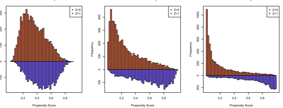
Figure C.1.1: Distributions of propensity scores under medium treatment prevalence, with good (left), moderate (middle), and poor (right) overlap.

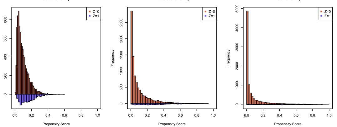
Figure C.1.2: Distributions of propensity scores under low prevalence of treatment, with good (left), moderate (middle), and poor (right) overlap.

We considered $\displaystyle(\beta_{1},\dots,$ $\displaystyle\beta_{6})=$ $\displaystyle\allowdisplaybreaks(0.15\gamma,$ $\displaystyle 0.3\gamma,$ $\displaystyle 0.3\gamma,$ $\displaystyle-0.2\gamma,$ $\displaystyle-0.25\gamma,$ $\displaystyle-0.25\gamma)$ and varied $\displaystyle\gamma$ from $\displaystyle 1$ to $\displaystyle 3$ for good, moderate, and poor overlap of PS distributions, as shown in Figure C.1.1. The intercept $\displaystyle\beta_{0}$ was chosen to reflect the prevalence of treatment as shown in Table C.1.1. We selected $\displaystyle\beta_{0}$ such that the prevalence is around $\displaystyle 0.10$ for low prevalence ($\displaystyle\beta_{0}=$ -2.1, -2.2, and -2.8 for good, moderate, and poor overlap respectively under low treatment prevalence), and the prevalence is around 0.40 for medium prevalence ($\displaystyle\beta_{0}=$ -0.1, 0, and 0.2 for good, moderate, and poor overlap respectively under medium treatment prevalence). The corresponding distributions of propensity scores is shown in Figure C.1.2. We generate $\displaystyle Y$ from the linear model $\displaystyle Y=0+\Delta Z-0.5X_{1}-0.5X_{2}-1.5X_{3}+0.8X_{4}+0.8X_{5}+X_{6}+\varepsilon$, where $\displaystyle\varepsilon\sim N(0,1.5)$ and $\displaystyle\Delta$ is the individual treatment effect. We choose, respectively, $\displaystyle\Delta=0.75$ (homogeneous treatment effect) and $\displaystyle e(\bm{X})^{2}+2e(\bm{X})+1$ (heterogeneous treatment effects), to compare the performance of the aforementioned methods. The results are summarized in Table C.1.2 (resp. Table C.1.3) for medium (resp. low) prevalence of treatment.

Table C.1.1: Average treatment prevalence for different levels of PS overlap.

	Overlap
Prevalence	Good	Moderate	Poor
Medium	40.08%	39.81%	39.63%
Low	10.26%	10.79%	10.24%

Table C.1.2: Treatment effect estimation (medium prevalence of treatment).

		Homogeneous treatment effect							Heterogeneous treatment effect
Weight	Overlap	True	ARB	RMSE	SD	SE	CP		True	ARB	RMSE	SD	SE	CP
IPW	Good	0.75	1.18	9.08	9.05	8.96	0.94		2.00	0.12	9.05	9.05	8.79	0.94
OW	Good	0.75	0.46	7.35	7.35	7.31	0.94		2.06	0.07	7.55	7.55	7.42	0.95
MW	Good	0.75	0.32	7.60	7.60	7.53	0.95		2.09	0.08	7.67	7.67	7.65	0.95
EW	Good	0.75	0.59	7.40	7.39	7.37	0.94		2.04	0.05	7.61	7.61	7.46	0.95
BW(11)	Good	0.75	0.06	10.73	10.74	10.74	0.95		2.20	0.05	10.40	10.40	10.85	0.96
BW(81)	Good	0.75	0.29	15.72	15.73	18.03	0.98		2.24	0.02	15.81	15.81	18.25	0.98
IPW	Mod	0.75	1.54	24.19	24.17	21.16	0.90		2.00	0.57	21.84	21.83	19.29	0.90
OW	Mod	0.75	1.05	8.36	8.33	8.40	0.94		2.13	0.05	8.92	8.93	8.73	0.94
MW	Mod	0.75	1.12	8.61	8.57	8.66	0.95		2.15	0.03	9.09	9.10	8.98	0.94
EW	Mod	0.75	0.91	8.57	8.54	8.67	0.95		2.11	0.05	9.18	9.18	8.94	0.94
BW(11)	Mod	0.75	1.43	13.08	13.04	13.28	0.96		2.24	0.08	13.14	13.15	13.57	0.96
BW(81)	Mod	0.75	0.15	20.87	20.88	24.83	0.98		2.25	0.25	20.82	20.82	25.15	0.98
IPW	Poor	0.75	6.49	55.46	55.27	41.21	0.79		2.05	2.34	49.06	48.85	36.51	0.81
OW	Poor	0.75	0.11	9.44	9.44	9.51	0.95		2.20	0.18	10.20	10.20	10.05	0.95
MW	Poor	0.75	0.36	9.74	9.75	9.79	0.95		2.21	0.22	10.51	10.50	10.31	0.95
EW	Poor	0.75	0.16	10.01	10.01	9.97	0.95		2.19	0.16	10.47	10.47	10.44	0.95
BW(11)	Poor	0.75	1.17	15.25	15.23	15.58	0.95		2.25	0.40	16.03	16.02	15.99	0.94
BW(81)	Poor	0.75	1.16	24.79	24.79	30.92	0.98		2.25	0.68	25.76	25.73	31.05	0.98

• These results are based on 1000 repetitions of the simulated data. Mod: Moderate; BW($\displaystyle\nu$): BW with $\displaystyle\nu=11$ and $\displaystyle 81$; ARB: absolute relative bias$\displaystyle\times 100$;

• RMSE: root mean-squared error$\displaystyle\times 100$; SD:empirical standard deviation$\displaystyle\times 100$; SE: average estimated standard error$\displaystyle\times 100$; CP: 95% coverage probability.

Table C.1.3: Treatment effect estimation (low prevalence of treatment).

		Homogeneous treatment effect							Heterogeneous treatment effect
Weight	Overlap	True	ARB	RMSE	SD	SE	CP		True	ARB	RMSE	SD	SE	CP
IPW	Good	0.75	1.18	25.59	25.59	24.55	0.93		1.21	0.91	25.54	25.53	24.31	0.92
OW	Good	0.75	0.59	11.28	11.27	11.47	0.96		1.31	0.06	11.83	11.83	11.57	0.94
MW	Good	0.75	0.59	11.72	11.72	11.99	0.96		1.34	0.03	12.34	12.34	12.00	0.95
EW	Good	0.75	0.52	11.87	11.87	12.02	0.96		1.29	0.08	12.35	12.36	12.14	0.95
BW(11)	Good	0.75	1.35	50.17	50.18	52.18	0.96		1.78	0.44	48.93	48.95	49.40	0.96
BW(81)	Good	0.75	6.74	167.78	167.79	151.60	0.80		2.16	2.21	162.19	162.20	142.24	0.80
IPW	Mod	0.75	11.33	70.11	69.63	51.24	0.78		1.26	7.40	64.79	64.15	48.29	0.76
OW	Mod	0.75	0.86	11.98	11.97	11.87	0.96		1.57	0.25	12.12	12.12	12.12	0.94
MW	Mod	0.75	0.68	12.51	12.50	12.50	0.95		1.64	0.25	12.87	12.87	12.61	0.94
EW	Mod	0.75	1.06	13.38	13.36	12.92	0.95		1.51	0.36	12.92	12.92	13.09	0.95
BW(11)	Mod	0.75	0.14	24.48	24.49	24.75	0.95		2.10	0.16	25.22	25.23	25.04	0.94
BW(81)	Mod	0.75	0.11	41.02	41.04	51.10	0.97		2.23	0.02	43.93	43.95	52.03	0.97
IPW	Poor	0.75	69.11	124.92	113.72	63.01	0.51		1.25	40.01	118.23	107.22	59.63	0.51
OW	Poor	0.75	0.50	13.54	13.54	13.58	0.94		1.71	0.46	13.88	13.86	13.98	0.96
MW	Poor	0.75	0.51	13.99	13.99	14.14	0.94		1.79	0.56	14.19	14.17	14.46	0.95
EW	Poor	0.75	0.17	14.75	14.76	14.72	0.94		1.64	0.52	15.14	15.12	15.04	0.95
BW(11)	Poor	0.75	0.24	24.07	24.09	25.45	0.96		2.16	1.06	24.89	24.80	26.04	0.96
BW(81)	Poor	0.75	2.08	40.43	40.42	53.75	0.99		2.24	1.52	41.84	41.72	54.04	0.98

• These results are based on 1000 repetitions of the simulated data. Mod: Moderate; BW($\displaystyle\nu$): BW with $\displaystyle\nu=11$ and $\displaystyle 81$; ARB: absolute relative bias$\displaystyle\times 100$;

• RMSE: root mean-squared error$\displaystyle\times 100$; SD:empirical standard deviation$\displaystyle\times 100$; SE: average estimated standard error$\displaystyle\times 100$; CP: 95% coverage probability.

References

- 1 Fonarow GC. Randomization—there is no substitute. JAMA cardiology 2016; 1(6): 633–635.
- 2 Freedman B. Equipoise and the ethics of clinical research. In: Routledge. 2017 (pp. 427–431).
- 3 Delgado-Rodríguez M, Llorca J. Bias. Journal of Epidemiology & Community Health 2004; 58(8): 635–641.
- 4 Dorn HF. Some problems arising in prospective and retrospective studies of the etiology of disease. New England Journal of Medicine 1959; 261(12): 571–579.
- 5 Fanaroff AC, Califf RM, Harrington RA, et al. Randomized trials versus common sense and clinical observation: JACC review topic of the week. Journal of the American College of Cardiology 2020; 76(5): 580–589.
- 6 Rubin DB. Matched sampling for causal effects. Cambridge University Press . 2006.
- 7 Hernán MA. With great data comes great responsibility: publishing comparative effectiveness research in epidemiology. Epidemiology (Cambridge, Mass.) 2011; 22(3): 290.
- 8 Hernán MA, Robins JM. Using big data to emulate a target trial when a randomized trial is not available. American journal of epidemiology 2016; 183(8): 758–764.
- 9 Hernán MA. Does water kill? A call for less casual causal inferences. Annals of epidemiology 2016; 26(10): 674–680.
- 10 Dahabreh IJ. Randomization, randomized trials, and analyses using observational data: A commentary on Deaton and Cartwright.. Social science & medicine (1982) 2018; 210: 41.
- 11 Rosenbaum PR, Rubin DB. The central role of the propensity score in observational studies for causal effects. Biometrika 1983; 70(1): 41–55.
- 12 Goetghebeur E, Cessie lS, De Stavola B, Moodie EE, Waernbaum I, and the topic group Causal Inference (TG7) of the STRATOS initiative . Formulating causal questions and principled statistical answers. Statistics in medicine 2020; 39(30): 4922–4948.
- 13 Ju C, Schwab J, Laan v. dMJ. On adaptive propensity score truncation in causal inference. Statistical methods in medical research 2018: 0962280218774817.
- 14 Cole SR, Hernán MA. Constructing inverse probability weights for marginal structural models. American journal of epidemiology 2008; 168(6): 656–664.
- 15 Hernan MA, Robins JM. Causal inference. CRC Boca Raton, FL: in press . 2023. Accessed: 2022-05-21.
- 16 Ridgeway G, McCaffrey D, Morral A, Burgette L, Griffin BA. Toolkit for Weighting and Analysis of Nonequivalent Groups: A tutorial for the twang package. Santa Monica, CA: RAND Corporation 2017.
- 17 Schafer JL, Kang J. Average causal effects from nonrandomized studies: a practical guide and simulated example.. Psychological methods 2008; 13(4): 279.
- 18 Khan S, Tamer E. Irregular identification, support conditions, and inverse weight estimation. Econometrica 2010; 78(6): 2021–2042.
- 19 Canavire-Bacarreza G, Castro Peñarrieta L, Ugarte Ontiveros D. Outliers in Semi-Parametric Estimation of Treatment Effects. Econometrics 2021; 9(2): 19.
- 20 Crump R, Hotz VJ, Imbens G, Mitnik O. Moving the goalposts: Addressing limited overlap in the estimation of average treatment effects by changing the estimand. 2006.
- 21 Crump RK, Hotz VJ, Imbens GW, Mitnik OA. Dealing with limited overlap in estimation of average treatment effects. Biometrika 2009; 96(1): 187–199.
- 22 Fogarty CB, Mikkelsen ME, Gaieski DF, Small DS. Discrete optimization for interpretable study populations and randomization inference in an observational study of severe sepsis mortality. Journal of the American Statistical Association 2016; 111(514): 447–458.
- 23 Heckman JJ, Vytlacil E. Policy-relevant treatment effects. American Economic Review 2001; 91(2): 107–111.
- 24 Imbens GW. Nonparametric estimation of average treatment effects under exogeneity: A review. Review of Economics and statistics 2004; 86(1): 4–29.
- 25 Einbeck J, Augustin T. On design-weighted local fitting and its relation to the Horvitz-Thompson estimator. Statistica Sinica 2009: 103–123.
- 26 Kang J, Chan W, Kim MO, Steiner PM. Practice of causal inference with the propensity of being zero or one: assessing the effect of arbitrary cutoffs of propensity scores. Communications for Statistical Applications and Methods 2016; 23(1): 1–20.
- 27 Schneeweiss S, Gagne J, Glynn R, Ruhl M, Rassen J. Assessing the comparative effectiveness of newly marketed medications: methodological challenges and implications for drug development. Clinical Pharmacology & Therapeutics 2011; 90(6): 777–790.
- 28 Busso M, DiNardo J, McCrary J. New evidence on the finite sample properties of propensity score reweighting and matching estimators. Review of Economics and Statistics 2014; 96(5): 885–897.
- 29 Vansteelandt S, Daniel RM. On regression adjustment for the propensity score. Statistics in medicine 2014; 33(23): 4053–4072.
- 30 Frölich M. Finite-sample properties of propensity-score matching and weighting estimators. Review of Economics and Statistics 2004; 86(1): 77–90.
- 31 Petersen ML, Porter KE, Gruber S, Wang Y, Laan v. dMJ. Diagnosing and responding to violations in the positivity assumption. Statistical methods in medical research 2012; 21(1): 31–54.
- 32 King G, Zeng L. The dangers of extreme counterfactuals. Political Analysis 2006; 14(2): 131–159.
- 33 Graham BS, Xavier Pinto dCC, Egel D. Inverse probability tilting for moment condition models with missing data. The Review of Economic Studies 2012; 79(3): 1053–1079.
- 34 Imai K, Ratkovic M. Covariate balancing propensity score. Journal of the Royal Statistical Society: Series B (Statistical Methodology) 2014; 76(1): 243–263.
- 35 Hainmueller J. Entropy balancing for causal effects: A multivariate reweighting method to produce balanced samples in observational studies. Political Analysis 2012; 20(1): 25–46.
- 36 Zubizarreta JR. Stable weights that balance covariates for estimation with incomplete outcome data. Journal of the American Statistical Association 2015; 110(511): 910–922.
- 37 Wong RK, Chan KCG. Kernel-based covariate functional balancing for observational studies. Biometrika 2017; 105(1): 199–213.
- 38 Hirshberg DA, Zubizarreta JR. On two approaches to weighting in causal inference. Epidemiology 2017; 28(6): 812–816.
- 39 Zhao Q. Covariate balancing propensity score by tailored loss functions. arXiv preprint arXiv:1601.05890 2016.
- 40 Hernán MA. Comment: Spherical cows in a vacuum: data analysis competitions for causal inference. Statistical Science 2019; 34(1): 69–71.
- 41 Robins JM, Hernan MA, Brumback B. Marginal Structural Models and Causal Inference in Epidemiology. Epidemiology 2000; 11(5): 550–560.
- 42 Hernán MÁ, Brumback B, Robins JM. Marginal structural models to estimate the causal effect of zidovudine on the survival of HIV-positive men. Epidemiology 2000: 561–570.
- 43 Ma X, Wang J. Robust inference using inverse probability weighting. Journal of the American Statistical Association 2020; 115(532): 1851–1860.
- 44 Zhou Y, Matsouaka RA, Thomas L. Propensity score weighting under limited overlap and model misspecification. Statistical Methods in Medical Research 2020; 29(12): 3721–3756.
- 45 Cole SR, Hernán MA, Robins JM, et al. Effect of highly active antiretroviral therapy on time to acquired immunodeficiency syndrome or death using marginal structural models. American Journal of Epidemiology 2003; 158(7): 687–694.
- 46 Stürmer T, Rothman KJ, Glynn RJ. Insights into different results from different causal contrasts in the presence of effect-measure modification. Pharmacoepidemiology and drug safety 2006; 15(10): 698–709.
- 47 Kurth T, Walker AM, Glynn RJ, et al. Results of multivariable logistic regression, propensity matching, propensity adjustment, and propensity-based weighting under conditions of nonuniform effect. American Journal of Epidemiology 2005; 163(3): 262–270.
- 48 Stürmer T, Rothman KJ, Avorn J, Glynn RJ. Treatment effects in the presence of unmeasured confounding: dealing with observations in the tails of the propensity score distribution—a simulation study. American journal of epidemiology 2010; 172(7): 843–854.
- 49 Lee BK, Lessler J, Stuart EA. Weight trimming and propensity score weighting. PloS one 2011; 6(3): e18174.
- 50 Li F, Thomas LE, Li F. Addressing extreme propensity scores via the overlap weights. American journal of epidemiology 2018; 188(1): 250–257.
- 51 Yang S, Ding P. Asymptotic inference of causal effects with observational studies trimmed by the estimated propensity scores. Biometrika 2018; 105(2): 487–493.
- 52 Li L, Greene T. A weighting analogue to pair matching in propensity score analysis. The international journal of biostatistics 2013; 9(2): 215–234.
- 53 Mao H, Li L, Greene T. Propensity score weighting analysis and treatment effect discovery. Statistical Methods in Medical Research 2018: 0962280218781171.
- 54 Li F, Morgan KL, Zaslavsky AM. Balancing covariates via propensity score weighting. Journal of the American Statistical Association 2018; 113(521): 390–400.
- 55 Hirano K, Imbens GW, Ridder G. Efficient estimation of average treatment effects using the estimated propensity score. Econometrica 2003; 71(4): 1161–1189.
- 56 Traskin M, Small DS. Defining the study population for an observational study to ensure sufficient overlap: a tree approach. Statistics in Biosciences 2011; 3(1): 94–118.
- 57 Tao Y, Fu H. Doubly robust estimation of the weighted average treatment effect for a target population. Statistics in medicine 2019; 38(3): 315–325.
- 58 Neyman J. Sur les applications de la théorie des probabilités aux experiences agricoles: Essai des principes. Roczniki Nauk Rolniczych 1923; 10: 1–51.
- 59 Imbens GW, Rubin DB. Causal inference in statistics, social, and biomedical sciences. Cambridge University Press . 2015.
- 60 Rosenbaum PR, Rubin DB. Reducing bias in observational studies using subclassification on the propensity score. Journal of the American statistical Association 1984; 79(387): 516–524.
- 61 Rubin DB. Estimating causal effects from large data sets using propensity scores. Annals of internal medicine 1997; 127(8_Part_2): 757–763.
- 62 Woo MJ, Reiter JP, Karr AF. Estimation of propensity scores using generalized additive models. Statistics in medicine 2008; 27(19): 3805–3816.
- 63 Lee BK, Lessler J, Stuart EA. Improving propensity score weighting using machine learning. Statistics in medicine 2010; 29(3): 337–346.
- 64 Kern HL, Stuart EA, Hill J, Green DP. Assessing methods for generalizing experimental impact estimates to target populations. Journal of research on educational effectiveness 2016; 9(1): 103–127.
- 65 Stuart EA, Rhodes A. Generalizing treatment effect estimates from sample to population: A case study in the difficulties of finding sufficient data. Evaluation review 2017; 41(4): 357–388.
- 66 Hájek J. Comment on a paper by D. Basu In: Godambe VP and Sprott DA (eds) Foundations of Statistical Inference. 1971.
- 67 Kang JD, Schafer JL, others . Demystifying double robustness: A comparison of alternative strategies for estimating a population mean from incomplete data. Statistical science 2007; 22(4): 523–539.
- 68 Robins JM. Marginal structural models versus structural nested models as tools for causal inference. In: Springer. 2000 (pp. 95–133).
- 69 Moodie EE, Saarela O, Stephens DA. A doubly robust weighting estimator of the average treatment effect on the treated. Stat 2018; 7(1): e205.
- 70 Geweke J. Bayesian inference in econometric models using Monte Carlo integration. Econometrica: Journal of the Econometric Society 1989: 1317–1339.
- 71 Robert CP, Casella G. Monte Carlo Statistical Methods. Springer Publishing Company, Incorporated . 2010.
- 72 McCaffrey DF, Ridgeway G, Morral AR. Propensity score estimation with boosted regression for evaluating causal effects in observational studies.. Psychological methods 2004; 9(4): 403.
- 73 Kish L. Survey sampling. 1965. New Yory: Wiley Pty Ltd 1985.
- 74 Lin W, others . Agnostic notes on regression adjustments to experimental data: Reexamining Freedman’s critique. The Annals of Applied Statistics 2013; 7(1): 295–318.
- 75 Robins J, Sued M, Lei-Gomez Q, Rotnitzky A. Comment: Performance of double-robust estimators when" inverse probability" weights are highly variable. Statistical Science 2007; 22(4): 544–559.
- 76 Westreich D, Edwards JK, Lesko CR, Stuart E, Cole SR. Transportability of trial results using inverse odds of sampling weights. American journal of epidemiology 2017; 186(8): 1010–1014.
- 77 Stuart EA. Matching methods for causal inference: A review and a look forward. Statistical science: a review journal of the Institute of Mathematical Statistics 2010; 25(1): 1.
- 78 Brennan JM, Thomas L, Cohen DJ, et al. Transcatheter versus surgical aortic valve replacement: propensity-matched comparison. Journal of the American College of Cardiology 2017; 70(4): 439–450.
- 79 Mao H, Li L. Flexible regression approach to propensity score analysis and its relationship with matching and weighting. Statistics in Medicine 2020.
- 80 Thomas LE, Li F, Pencina MJ. Overlap Weighting: A Propensity Score Method That Mimics Attributes of a Randomized Clinical Trial. Jama 2020.
- 81 Lockhart M, Hill SJ, Merolla J, Romero M, Kousser T. America’s electorate is increasingly polarized along partisan lines about voting by mail during the COVID-19 crisis. Proceedings of the National Academy of Sciences 2020; 117(40): 24640–24642.
- 82 Butters R, Hare C. Polarized Networks? New Evidence on American Voters’ Political Discussion Networks. Political Behavior 2020: 1–25.
- 83 Barsky R, Bound J, Charles KK, Lupton JP. Accounting for the black–white wealth gap: a nonparametric approach. Journal of the American statistical Association 2002; 97(459): 663–673.
- 84 Walker AM, Patrick AR, Lauer MS, et al. A tool for assessing the feasibility of comparative effectiveness research. Comp Eff Res 2013; 3: 11–20.
- 85 Yoshida K, Solomon DH, Haneuse S, et al. A tool for empirical equipoise assessment in multigroup comparative effectiveness research. Pharmacoepidemiology and drug safety 2019.
- 86 Dehejia RH, Wahba S. Causal effects in nonexperimental studies: Reevaluating the evaluation of training programs. Journal of the American statistical Association 1999; 94(448): 1053–1062.
- 87 Schneider EC, Cleary PD, Zaslavsky AM, Epstein AM. Racial disparity in influenza vaccination: does managed care narrow the gap between African Americans and whites?. Jama 2001; 286(12): 1455–1460.
- 88 Breiman L, Friedman J, Stone C, Olshen R. Classification and Regression Trees. The Wadsworth and Brooks-Cole statistics-probability seriesTaylor & Francis . 1984.
- 89 Hastie T, Tibshirani R, Friedman J. The Elements of Statistical Learning: Data mining, Inference and Prediction. New York: Springer. 2nd ed ed. 2009.
- 90 Johnson D. The triangular distribution as a proxy for the beta distribution in risk analysis. Journal of the Royal Statistical Society: Series D (The Statistician) 1997; 46(3): 387–398.
- 91 Shaikh AM, Simonsen M, Vytlacil EJ, Yildiz N. A specification test for the propensity score using its distribution conditional on participation. Journal of Econometrics 2009; 151(1): 33–46.
- 92 Rubin DB. Using propensity scores to help design observational studies: application to the tobacco litigation. Health Services and Outcomes Research Methodology 2001; 2(3-4): 169–188.
- 93 Robins JM, Rotnitzky A, Zhao LP. Estimation of regression coefficients when some regressors are not always observed. Journal of the American statistical Association 1994; 89(427): 846–866.
- 94 Tsiatis A. Semiparametric theory and missing data. Springer Science & Business Media . 2007.
- 95 Léger M, Chatton A, Le Borgne F, Pirracchio R, Lasocki S, Foucher Y. Causal inference in case of near-violation of positivity: comparison of methods. Biometrical Journal 2022.
- 96 Moodie EE, Stephens DA, Wallace MP. G-Estimation. Wiley StatsRef: Statistics Reference Online 2014: 1–8.
- 97 Ma S, Kosorok MR. Robust semiparametric M-estimation and the weighted bootstrap. Journal of Multivariate Analysis 2005; 96(1): 190–217.
- 98 Lunceford JK, Davidian M. Stratification and weighting via the propensity score in estimation of causal treatment effects: a comparative study. Statistics in medicine 2004; 23(19): 2937–2960.
- 99 Stefanski LA, Boos DD. The calculus of M-estimation. The American Statistician 2002; 56(1): 29–38.
- 100 Wooldridge JM. Inverse probability weighted M-estimators for sample selection, attrition, and stratification. Portuguese Economic Journal 2002; 1(2): 117–139.
- 101 Cheng G, Yu Z, Huang JZ. The cluster bootstrap consistency in generalized estimating equations. Journal of Multivariate Analysis 2013; 115: 33–47.
- 102 Romano JP, Wolf M. Subsampling inference for the mean in the heavy-tailed case. Metrika 1999; 50(1): 55–69.
- 103 Zhao Q, Small DS, Bhattacharya BB. Sensitivity analysis for inverse probability weighting estimators via the percentile bootstrap. Journal of the Royal Statistical Society: Series B (Statistical Methodology) 2019; 81(4): 735–761.
- 104 Rosner B. Fundamentals of biostatistics. 2016.
- 105 Hong H, Leung MP, Li J. Inference on finite-population treatment effects under limited overlap. The Econometrics Journal 2020; 23(1): 32–47.
- 106 Zhou T, Tong G, Li F, Thomas LE. PSweight: An R package for propensity score weighting analysis. arXiv preprint arXiv:2010.08893 2020.
- 107 Digitale JC, Martin JN, Glymour MM. Tutorial on directed acyclic graphs. Journal of Clinical Epidemiology 2022; 142: 264–267.
- 108 Diemer EW, Hudson JI, Javaras KN. More (adjustment) is not always better: How directed acyclic graphs can help researchers decide which covariates to include in models for the causal relationship between an exposure and an outcome in observational research. Psychotherapy and Psychosomatics 2021; 90(5): 289–298.
- 109 Tan Z. Comment: Understanding or, ps and dr. Statistical Science 2007; 22(4): 560–568.
- 110 Mercatanti A, Li F, others . Do debit cards increase household spending? Evidence from a semiparametric causal analysis of a survey. The Annals of Applied Statistics 2014; 8(4): 2485–2508.
- 111 Gut A. Probability: a graduate course. 75. Springer Science & Business Media . 2012.
- 112 Newey WK. The asymptotic variance of semiparametric estimators. Econometrica: Journal of the Econometric Society 1994: 1349–1382.