Sim-to-Real Learning of All Common Bipedal Gaits
via Periodic Reward Composition

Abstract

We study the problem of realizing the full spectrum of bipedal locomotion on a real robot with sim-to-real reinforcement learning (RL). A key challenge of learning legged locomotion is describing different gaits, via reward functions, in a way that is intuitive for the designer and specific enough to reliably learn the gait across different initial random seeds or hyperparameters. A common approach is to use reference motions (e.g. trajectories of joint positions) to guide learning. However, finding high-quality reference motions can be difficult and the trajectories themselves narrowly constrain the space of learned motion. At the other extreme, reference-free reward functions are often underspecified (e.g. move forward) leading to massive variance in policy behavior, or are the product of significant reward-shaping via trial-and-error, making them exclusive to specific gaits. In this work, we propose a reward-specification framework based on composing simple probabilistic periodic costs on basic forces and velocities. We instantiate this framework to define a parametric reward function with intuitive settings for all common bipedal gaits - standing, walking, hopping, running, and skipping. Using this function we demonstrate successful sim-to-real transfer of the learned gaits to the bipedal robot Cassie, as well as a generic policy that can transition between all of the two-beat gaits.

I Introduction

Using reinforcement learning (RL) to learn all of the common bipedal gaits found in nature for a real robot is an unsolved problem. A key challenge of learning a specific locomotion gait via RL is to communicate the gait behavior through the reward function. In general, a specific gait can be viewed as a dynamic process that has a characteristic periodic structure, but is also able to flexibly adapt to moderate environment disturbances. This suggests two considerations when designing a gait reward function. First, the reward must be specific enough to produce the desired gait characteristic when optimized. Second, to account for the fact that there is uncertainty about the exact details of a gait in the context of specific terrain and dynamic conditions, the reward should not be overly constraining.

The common use of reference trajectories to specify gait-specific rewards, e.g., [1, 2, 3, 4, 5], partly addresses the first consideration above, but mostly ignores the second. In particular, a reference trajectory only captures a small part of the variation needed to realize a gait characteristic under varying conditions. Thus, attempting to adhere to such a trajectory can prevent learning a characteristic gait that is more robust and/or efficient, not to mention that deriving feasible reference trajectories for a particular desired gait can be very challenging in the first place.

Reference-free approaches to specifying reward functions for locomotion are often highly underspecified, for example, those used in the OpenAI Gym [6] locomotion benchmarks. With this starting point, achieving a specific gait characteristic requires iterations of heuristic reward-function adjustments, based on observed RL performance, until arriving at a desired behavior. This approach can be tedious when it works and is unreliable as a general framework. Other reference-free approaches structure the reward around a specific type of locomotion behavior [7] without being easily extended to other behaviors.

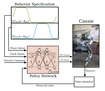
Figure 1: In this work, we present a reward design framework which makes it easy to learn policies which can stand, walk, run, gallop, hop, and skip on hardware. We condition the reward function based on a number of gait parameters, and also provide these parameters to the LSTM policy, which outputs PD joint position targets and PD gains to the robot.

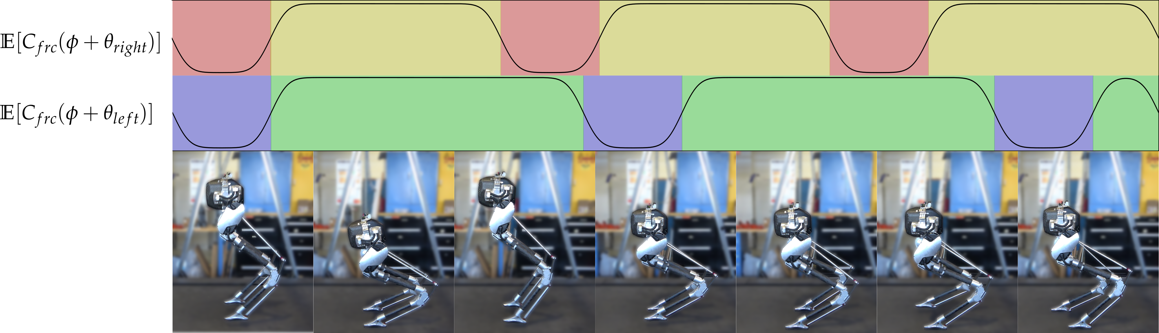
Figure 2: A series of images showing a neural network policy controlling Cassie and continuously transitioning from hopping to galloping to walking. We present a simple reward design paradigm which makes use of probabilistic intervals to apply cost functions at specific times, allowing policies to learn all common bipedal gaits exhibited by animals in nature.

The first contribution of our work is to present a principled framework for designing reward functions that can naturally capture all of the periodic bipedal locomotion gaits. We are motivated by the fact that all common bipedal gaits can be defined by periodic swing phases (foot swinging in the air) and stance phases (foot planted on the ground) for each foot [8]. A fundamental distinction between swing and stance phases is the complementary presence and absence of foot forces and foot velocities for a given foot. We can create principled reward functions based on this observation by using the magnitudes of foot forces and velocities such that during a swing phase, forces are penalized while velocities are allowed, prompting the policy to learn to lift the foot. Thus, our framework describes gaits as a sequence of periodic phases, each of which rewards or penalizes a particular measurement of the physical system. Our hypothesis is that this framework will allow for a more natural specification of reward functions that sufficiently constrain RL to learn the desired gait characteristics, while allowing for flexible adaptation to specific environmental disturbances.

Our second contribution is to demonstrate this framework for sim-to-real RL of all common bipedal gaits, including walking, running, galloping, skipping, and hopping, without using a motion capture dataset or reference trajectories. We train policies for each of these behaviors in simulation and successfully demonstrate them on hardware. Further, by providing the framework’s gait parameters as a command input to the policy, we are able to learn a multi-gait policy which can hop, gallop, run, and walk.

II Background

The practice of synthesizing locomotion behaviors has been studied in a variety of fields. In character animation, kinematics-based approaches (i.e., those using motion capture data) are commonly used to synthesize locomotion [9] [10] [11], with some newer approaches using deep learning [1] to train neural networks to solve problems like adapting realistically to varying ground geometries [12] [13] or blending several types of actions into one realistic body motion [2]. Physics-based character animation, wherein the pose of a character is controlled through the application of torques and motions are simulated using a physics engine, has also come into prominence in recent years [14], though is notably more difficult to use effectively for complicated motions [15] when compared to kinematics-based methods.

Approaches which use reinforcement learning to synthesize locomotion bear heavy similarities to the aforementioned methods used in character animation. Much recent work uses trajectory-matching reward functions to train policies to imitate some reference trajectory (akin to a motion capture) while subjecting the policies to simulated physics, resulting in policies that behave realistically while imitating some reference trajectory [16] [5] [3] [17] [4]. Reinforcement learning has also been used for synthesizing locomotion without the use of reference trajectories, but these approaches often place little emphasis on subjective quality of behaviors, resulting in behaviors which maximize some objective while producing policies which are often inefficient, infeasible or unsafe to execute in the real world, and not usually visually pleasing [6] [18]. Methods which do prioritize physically realistic behavior without using a reference trajectory exist [19] [20] [7], but their reward functions are specific to single behaviors and are not trivial to extend to other behaviors.

III Learning Bipedal Gaits with Periodic Reward Composition

III-A Reinforcement Learning Framework

We formulate our problem in the framework of reinforcement learning (RL) [21], for which we assume basic familiarity. The world is modeled as a discrete-time Markov Decision Process (MDP) with continuous state space $S$, continuous action space $A$, transition function $T(s,a,s^{\prime})$, and reward function $R(s,t)$. Here $T(s,a,s^{\prime})$ gives the probability density over the next state $s^{\prime}$ after taking action $a$ in state $s$, and $R(s,t)$ gives the non-stationary reward for being in state $s$ at time step $t$.

A control policy is a possibly stochastic mapping $\pi(a\;|\;s)$ from states to actions, which dictates behavior. Given a policy the expected $T$-horizon discounted return is given by $J(\pi)=\mathbb{E}\left[\sum_{t=0}^{T}\gamma^{t}R(S_{t},t)\right]$, where $\gamma\in[0,1]$ is a discount factor and $S_{t}$ is a random variable representing the state at time $t$ when following policy $\pi$ under transition dynamics $T$. The goal of RL is to learn a policy $\pi$ that maximizes $J(\pi)$ based on trial-and-error training experience in the world. In this work, we follow a sim-to-real RL paradigm where training is done in simulation to identify a policy, which is then used in the real-world.

III-B Periodic Reward Composition

Since our framework is targeted toward periodic behaviors, we index time via a cycle time $\phi$ variable, which repeatedly cycles over a normalized time period of $[0,1]$ at discrete time steps rather than increasing monotonically. Accordingly, the non-stationary reward function $R(s,\phi)$ is periodic and defined in terms of $\phi$ rather than absolute time.

As motivated in the introduction, our framework specifies rewards in terms of compositions of rewards on periodic intervals. We define the reward as a biased sum of $n$ reward components $R_{i}(s,\phi)$, where each component $R_{i}(s,\phi)$ captures a desired characteristic of the gait during a particular phase.

$$R(s,\phi)=\beta+\sum_{i}R_{i}(s,\phi)$$

Each reward component $R_{i}(s,\phi)$ is a product of a phase coefficient $c_{i}$, a phase indicator $I_{i}(\phi)$, and a real-valued phase reward measurement $q_{i}(s)$ (e.g. norm of a foot force).

$$R_{i}(s,\phi) =c_{i}\cdot I_{i}(\phi)\cdot q_{i}(s)$$

The phase coefficient $c_{i}$ is a scalar whose sign determines the effect that the phase measurement $q_{i}(s)$ has on the total reward during cycle times when the reward component is active. The phase indicator function $I_{i}(\phi)$ is a binary-valued random variable denoting whether the target phase is active or not at cycle time $\phi$. In this work, the distribution of each $I_{i}$ is described by random variables $A_{i}$ and $B_{i}$ representing the start and end times of the period respectively. Since $A_{i}$ and $B_{i}$ represent intervals on a cycle, we use Von Mises distributions (approximations of the wrapped Normal distribution) described by the parameter tuple $(a_{i},b_{i},\kappa)$, which gives the means $a_{i}$ and $b_{i}$ and shared variance parameter $\kappa$. The distribution of the binary phase indicator $I_{i}(\phi)$ is then simply:

$$P\left(I_{i}(\phi)=x\right)= \begin{cases}P(A_{i}<\phi<B_{i})&\text{if $x=1$}\\ 1-P(A_{i}<\phi<B_{i})&\text{if $x=0$}\end{cases}$$ (1)

where $$P(A_{i}<\phi<B_{i})=P(A_{i}<\phi)(1-P(B_{i}<\phi))$$

$$A_{i}\sim\boldsymbol{\Phi}(2\pi a_{i},\kappa)\text{ and }B_{i}\sim\boldsymbol{\Phi}(2\pi b_{i},\kappa)$$

$$\boldsymbol{\Phi}\text{ is the Von Mises distribution }$$

Note that this formulation allows for uncertainty about the exact start and end of each phase to be captured via the variance parameter $\kappa$ of the Von Mises distributions. This has a smoothing effect on the reward function at phase boundaries, which we have found to usefully encourage more stable and consistent learning. While we could directly use this probabilistic reward function $R(s,\phi)$ for RL training by sampling from the reward distribution at each step, we instead apply RL to the deterministic expectation of $R(s,\phi)$.

$$\mathbb{E}\left[R(s,\phi)\right] =\sum_{i}^{n}c_{i}\cdot\mathbb{E}[I_{i}(\phi)]\cdot q_{i}(s)+\beta$$

Due to the linearity of expectations, for any policy $\pi$ the expected cumulative return $J(\pi)$ is the same regardless of whether we use stochastic rewards or their expectations.

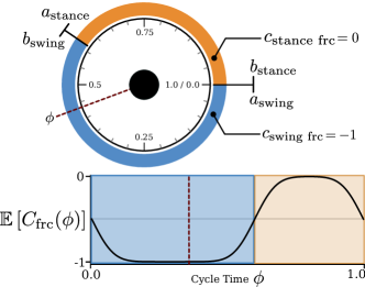
Figure 3: The circular intervals of two phases, swing and stance, are shown on a polar plot. The expected sum of the phase indicators and phase coefficients for foot force $C_{\text{frc}}(\phi)$ is shown below.

III-C Describing Bipedal Gaits

For simplicity, we begin by describing repeatedly lifting and placing a single foot, or equivalently, cycling between swing and stance phases with our framework. As our phase reward measurements, we select the norm of foot force $q_{\text{frc}}(s)$ and the norm of foot velocity $q_{\text{spd}}(s)$. During the swing phase we want to penalize foot forces and ignore foot velocities, so we choose $c_{\text{swing frc}}=-1$ and $c_{\text{swing spd}}=0$. Similarly, we choose $c_{\text{stance spd}}=-1$ and $c_{\text{stance frc}}=0$ to penalize foot velocities and ignore foot forces during the stance phase. We constrain the swing and stance phases to follow immediately after one another and together last the entire cycle time by defining a ratio $r\in(0,1)$ and setting the intervals for both phases such that the swing phase lasts length $r$, while the stance phase lasts length $1-r$ and starts directly afterwards. Finally, by choosing a common scale $\kappa$, we can define the indicator functions $I_{\text{frc}}(\phi)$ and $I_{\text{spd}}(\phi)$ by using Equation 1.

For convenience, we define $C_{\text{frc}}(\phi)$ and $C_{\text{spd}}(\phi)$ as the expected sum of the product of all the phase indicators and phase coefficients for the swing and stance phases:

$$\mathbb{E}\left[C_{\text{frc}}(\phi)\right] = c_{\text{swing frc}}\cdot\mathbb{E}[I_{\text{swing frc}}(\phi)]$$

$$+ c_{\text{stance frc}}\cdot\mathbb{E}[I_{\text{stance frc}}(\phi)]$$

$$\mathbb{E}\left[C_{\text{spd}}(\phi)\right] = c_{\text{swing spd}}\cdot\mathbb{E}[I_{\text{swing spd}}(\phi)]$$

$$+ c_{\text{stance spd}}\cdot\mathbb{E}[I_{\text{stance spd}}(\phi)]$$

Refer to Fig.3 for a visual explanation of the phase start and end times, $\phi$, and the expected value of $C_{\text{frc}}$. For more complicated behaviors, we find that visualizing $C_{\text{frc}}(\phi)$ can be useful for understanding how the reward function changes over the cycle to guide the learning of a particular behavior.

Putting the force and speed components together, the expected overall reward for repeatedly lifting and placing a single foot is

$$\mathbb{E}\left[R_{\text{unipedal}}(s,\phi)\right] = \mathbb{E}\left[C_{\text{frc}}(\phi)\right]\cdot q_{\text{frc}}(s)$$

$$+ \mathbb{E}\left[C_{\text{spd}}(\phi)\right]\cdot q_{\text{spd}}(s)$$

Bipedal gaits are behaviors where the left and right feet both follow the same sequence of phases described above, but offset relative to each other in phase time. For instance, in a walking behavior the timings of the swing and stance phases are shifted apart by half of the period length (one leg in swing, the other in stance), while a hopping behavior is one where both feet synchronously enter the swing and stance phases. To expand the simple behavior of lifting and placing a single foot into the full spectrum of bipedal gaits, we need only introduce two cycle offset parameters $\theta_{\text{left}},\theta_{\text{right}}$ which define the exact timing shift between the identical sequence of behavioral phases for the left and right feet, and differentiate between the norms of left and right foot forces, $q_{\text{left frc}}(s),\ q_{\text{right frc}}(s)$ and norms of left and right foot velocities $q_{\text{left spd}}(s),\ q_{\text{right spd}}(s)$. The expected overall reward for a bipedal behavior is

$$\mathbb{E}[R_{\text{bipedal}}(s,\phi)] = \mathbb{E}[C_{\text{frc}}(\phi+\theta_{\text{left}})]\cdot q_{\text{left frc}}(s)$$ (2)

$$+ \mathbb{E}[C_{\text{frc}}(\phi+\theta_{\text{right}})]\cdot q_{\text{right frc}}(s)$$

$$+ \mathbb{E}[C_{\text{spd}}(\phi+\theta_{\text{left}})]\cdot q_{\text{left spd}}(s)$$

$$+ \mathbb{E}[C_{\text{spd}}(\phi+\theta_{\text{right}})]\cdot q_{\text{right spd}}(s)$$

Introducing $\theta_{\text{left}},\theta_{\text{right}}$ for two phase behaviors allows us to define reward functions for walking, galloping, and hopping. Additionally, by using four phases rather than two in each component, we can derive a skipping reward function, as shown in Fig. 4.

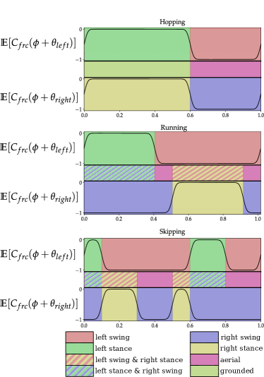
Figure 4: Plot of the expected value of the force phase coefficient for each foot for some example bipedal gaits. In hopping there is a $|\theta_{\text{left}}-\theta_{\text{right}}|\approx 0$ shift between the left and right feet. For walking and running, $|\theta_{\text{left}}-\theta_{\text{right}}|\approx 0.5$, with transitional shifts resulting in galloping. Four phases are necessary for describing skipping, as well as a $|\theta_{\text{left}}-\theta_{\text{right}}|\approx 0.5$ shift between the left and right feet. The shaded region between the phase coefficient plots show the hybrid phases from combining the left and right foot behaviors together.

IV Method

Network Architecture and Action Space: For all policies, we use a Long Short-Term Memory neural network [22] with two recurrent hidden layers of size 128 each, and a simple linear output projection of size 30, corresponding to 10 desired joint positions, and 10 sets of PD gains, as seen in Fig. 1. The desired joint positions are added to a set of constant offsets corresponding to a neutral standing position, such that an output vector of zeroes results in a standing pose. Similarly, the P gains and D gains are also summed with a fixed ’neutral’ set of gains. The policy is evaluated at 40Hz, and the robot’s PD controllers are run at 2000Hz. A similar system is used in [3] and [4], though without PD gain deltas.

State Space: To prevent the reinforcement learning environment from becoming a non-stationary Markov decision process, some information about the periodic reward function must be present in the state provided to the policy. Specifically, the policy must receive some sort of encoding of the current cycle time $\phi$, an encoding of the cycle offset parameters, $\theta_{\text{left}},\theta_{\text{right}}$, and information about the start and end times of the phases of the phase reward components.

In order to encode the current cycle time $\phi$ and the cycle offset parameters $\theta_{\text{left}},\theta_{\text{right}}$, we condition the policies on two clock inputs:

$$p=\left\{\sin\left(\frac{2\pi(\phi+\theta_{\text{left}})}{L}\right),\sin\left(\frac{2\pi(\phi+\theta_{\text{right}})}{L}\right)\right\}$$

where $L$ is the number of discrete timesteps in the entire cycle. To encode information about the start and end times of the phases into the state, we derive a vector of ratios from the sequence of phase timings; each ratio represents the proportion out of the total period that a phase occupies. For instance, a phase $j$ with start time $a_{i,j=0.3}$ and end time $b_{i,j}=0.7$ should occupy 40% of the total period time (plus or minus some uncertainty); thus, we can derive a ratio $r_{j}=0.4$. Each phase’s ratio is calculated and provided to the policy.

Thus, the policy’s input consists of:

$$X_{t}=\left\{\begin{array}[]{ll}\hat{q},\ \hat{\dot{q}}&\text{robot state}\\ \vskip 3.0pt plus 1.0pt minus 1.0pt\dot{x}_{\text{desired}},\dot{y}_{\text{desired}}&\text{desired velocity}\\ r,p&\text{phase ratios and clock inputs}\\ \end{array}\right.$$

Where $\hat{q},\hat{\dot{q}}$ are estimates of the pelvis orientation, rotational velocity, joint positions and joint velocities. $\dot{x}_{\text{desired}}$ and $\dot{y}_{\text{desired}}$ are speed commands randomized during training, and manually controlled by the user during evaluation.

Reward Formulation: We use the set of reward components from $R_{\text{bipedal}}$ defined in Equation 2 to learn single-gait policies. In addition, we also use a variety of auxiliary cost components to further constrain the path of viable exploration towards stable locomotion and facilitate successful sim-to-real transfer as well as command the policy to match a desired orientation, forward speed, and sidespeed. These rewards do not need to vary as a function of time, and can be seen as a special case of the reward component framework, wherein the random variable $c_{i}$ has only one phase, and thus one possible value (in this case, $-1$, to show that we wish to penalize these quantities $q_{i}$ for the entire period).

$$R_{\text{cmd}}(s) = (-1)\cdot q_{\dot{x}}(s)$$

$$+ (-1)\cdot q_{\dot{y}}(s)$$

$$+ (-1)\cdot q_{\text{orientation}}(s)$$

$$R_{\text{smooth}}(s) = (-1)\cdot q_{\text{action diff}}(s)$$

$$+ (-1)\cdot q_{\text{torque}}(s)$$

$$+ (-1)\cdot q_{\text{pelvis acc}}(s)$$

$$\mathbb{E}[R(s,\phi)]=\mathbb{E}[R_{\text{bipedal}}(s,\phi)]+R_{\text{smooth}}(s)]+R_{\text{cmd}}(s)+\beta$$ (3)

Where $q_{\dot{x}}$ and $q_{\dot{y}}$ are measures of error between the commanded velocity and the actual pelvis velocity, and $q_{\text{orientation}}$ is the negative exponent of quaternion difference between the pelvis orientation and an orientation which faces straight, which can be used to change the heading of the robot. $q_{\text{pelvis acc}}$ is a cost for aggressive pelvis motion, which helps reduce noise in the state estimator, while $q_{\text{action diff}}$ is a cost for aggressive actions and $q_{\text{torque}}$ is an overall joint torque cost to encourage efficient motions. For general policies which can learn and transition between a continuum of bipedal gaits, we specify additional reward terms which are discussed in Section V.

Dynamics Randomization: In order to facilitate successful sim-to-real transfer, we use dynamics randomization [23] [24] to expose the policies to a wide variety of possible real-world dynamics. Specifically, we randomize the execution rate of the policy, the mass and damping of the joints, the friction of the ground, the slope of the ground, and joint position encoder noise. Details on the ranges and distributions used to randomize these parameters can be found in Table I. These parameters are randomized at the beginning of every rollout during training and remain constant throughout each rollout.

Parameter	Unit	Range
Joint damping	Nms/rad	$[0.3,4.0]\times\text{default values}$
Joint mass	kg	$[0.5,1.5]\times\text{default values}$
Ground Friction	–	$[0.35,1.1]$
Ground Slope	rad	$[-0.03,0.03]$
Joint Encoder Offset	rad	$[-0.05,0.05]$

Table I: The ranges for randomization of several dynamics parameters during training. We use a uniform distribution over the given ranges for all listed parameters.

Proximal Policy Optimization: To train our policies, we use a common model-free reinforcement learning algorithm known as Proximal Policy Optimization (PPO) [25]. More specifically, we use the recurrent adaptation described in [4], which samples batches of trajectories from a replay buffer, rather than batches of individual timesteps. In our case, we use a recurrent critic with exactly the same dimensions as the actor with the exception of the final linear output vector, which in the case of the critic is a scalar. We use a fixed exploration action noise, with standard deviation $e^{-1}$. In addition, we incorporate a mirror loss term [26] into our policy gradient algorithm with the aim of achieving more symmetric locomotion behavior.

V Experimental Results

Training Details. Policies were trained using PPO with a batch size of 32 trajectories of up to 300 timesteps each, a learning rate of $0.0001$ for both the actor and critic, a replay buffer of 50,000 samples, and 4 epochs per iteration. Training was terminated after 150,000,000 samples, which took between 24 and 36 hours per policy. We use the cassie-mujoco-sim [27] simulator, based on MuJoCo [28], to simulate Cassie during training.

Single-Gait Policy Results. We found that it was straightforward to use the probabilistic framework to train policies to learn standalone gaits, such as hopping, walking, running, or even skipping. These behaviors can be learned simply by holding the values of ratios $r$ and cycle offset parameters $\theta_{\text{left}},\theta_{\text{right}}$ to be constant throughout training (we refer the reader to Fig. 4 for examples of gait specifications). Videos of single-gait policies which learn skipping hopping, and walking can be found in our submission video.

Multi-Gait Policy Results By keeping the cycle offsets fixed and varying the phase ratios over some range during training, we are able to train policies that can learn to hop with more or less time in the air, and policies that can transition from walking to running. However, learning to transition between gaits by varying both the cycle offsets and phase ratios during training appears to be a challenging learning problem: policies which are trained in this fashion can end up asymmetrically walking instead of hopping, or learn other undesirable behaviors that resemble a fusion of all the different commanded gaits. To avoid these issues, we introduce additional reward terms called transition penalties to further distinguish each of the desired behaviors from each other during training. Transition penalties are behavior-specific costs which are only active when specific behaviors are being commanded. For hopping, which is commanded when cycle offsets are very close to each other, we activate a cost for constraining the feet positions to be close together. Similarly, by adding another transition penalty for standing, we can train a generic controller to transition between all steady state two-beat gaits and standing in place. Full details of the reward function for generic controllers are described in detail in the Appendix.

Outdoor Experiments We demonstrate the robustness of policies learned with our approach in a variety of outdoor experiments, shown in our submission video . Given that the robot is effectively blind to the external world, the behaviors we observe in response to disturbances are surprisingly robust. We show the multi-gait policy hopping on and off a sidewalk, walking with one foot elevated on a curb, and running over small bumps in its path. The policy is also shown smoothly transitioning between all of the 2-beat gaits while moving forward on a crowned road, and while turning in a small circle on a turf field. We also show a multi-gait policy descending down 5 steps of stairs while in a running gait. In the staircase and sidewalk tests, we observe the foot slipping off of small ledges and being compliant to the slope of the ground. This indicates a priority on force profile, as opposed to position only.

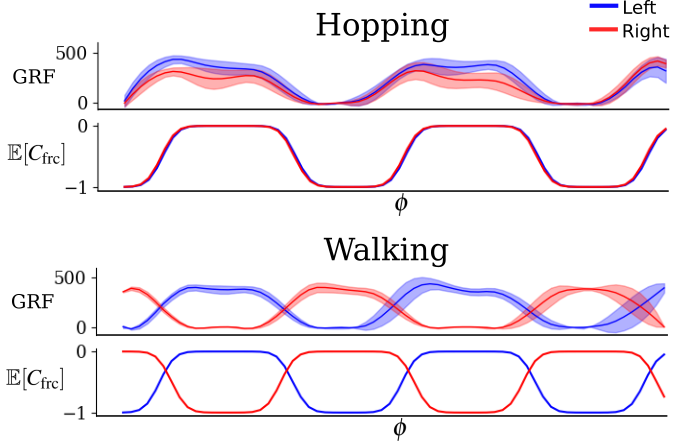
Figure 5: Comparison between the mean measured simulation ground reaction forces (GRFs) in newtons and the corresponding expected values of $C_{\text{frc}}$ over multiple policies. When the expectation is close to -1, the policies refrain from applying foot forces. When the expectation is close to 0, the policies apply foot forces.

VI Conclusion

In this work, we introduced a probabilistic reward framework which allows for learning of all of the common bipedal gait behaviors observed in animals. This framework requires no reference trajectories, enabling policies to explore a rich space of possible interaction with the world during training without artificial constraints to some arbitrary trajectory through space. We showed that not only are we able to train policies to learn all common bipedal gaits individually, including walking, running, hopping, galloping, and skipping, but also that we can learn all 2-beat behaviors on single policies and transition between them continuously, even while in motion. Some questions which remain unanswered include how easily this framework might be applied to the space of possible quadrupedal gaits, or other bipedal morphologies. A modified version of this framework could also be applied to aperiodic motions to learn one-off behaviors.

Appendix

Full Reward Functions for Generic 2-Beat Policies

When learning the continuum of 2-beat gaits, we find that policies often learn to stutter rather than hop with their feet together, which is not observed when training hopping standalone. To combat this, we introduce a hop symmetry term, a cost which becomes active when the cycle offsets of both legs match closely and punishes large distances between the feet in the sagittal and transverse planes, $\text{err}_{\text{sym}}$,

$$q_{\textit{hop sym}}(s)=1-\exp(-\text{err}_{\text{sym}}\exp(-5\left|sin(2\pi(\theta_{\text{left}}-\theta_{\text{right}}))\right|))$$

To learn a standing behavior in addition to the rest of the 2-beat gaits, the reward function must be modified to reflect our wish for the policy to remain very still when commanded. First, we define the standing region of gait parameter space as one where the swing-to-stance phase ratio is close to 0.

We define $\omega=(1+\exp(-50(r_{\text{swing}}-0.15)))^{-1}$, which is a coefficient close to one during normal locomotion (when the swing and stance ratios are in the range [0.35, 0.7], and close to zero during standing (where the swing phase ratio is close to zero). Now we define an additional standing cost, which applies an additional action difference cost and a foot symmetry cost (similar to the hopping symmetry) when the command inputs are in the standing region.

$$q_{\text{standing cost}}(s)=1-\exp(-((\text{err}_{\text{sym}})+20q_{\text{action diff}}(s)))$$

Now we define the full reward for a generic policy which includes standing:

$$\mathbb{E}[R_{\text{multi}}(s,\phi)] = 0.400 \cdot\mathbb{E}[R_{\text{bipedal}}(s,\phi)]$$

$$\ + 0.300 \cdot\mathbb{E}[R_{\text{cmd}}(s)]$$

$$\ + 0.100 \cdot\mathbb{E}[R_{\text{smooth}}(s)]$$

$$\ + 0.100 \cdot(\omega-1)\cdot q_{\text{standing cost}}(s)$$

$$\ + 0.100 \cdot(-1)\cdot q_{\text{hop sym}}(s)$$

$$\ + 1$$

Quantity $q_{i}$	Detail
$q_{\text{left/right frc}}$	$1-\exp(-\omega\|\text{raw\_foot\_frc}\|_{2}^{2}/100)$
$q_{\text{left/right spd}}$	$1-\exp(-2\cdot\omega\|\text{raw\_foot\_spd}\|_{2}^{2})$
$q_{\dot{x}}$	$1-\exp(-2\cdot\omega|\dot{x}_{\text{desired}}-\dot{x}_{\text{actual}}|)$
$q_{\dot{y}}$	$1-\exp(-2\cdot\omega|\dot{y}_{\text{desired}}-\dot{y}_{\text{actual}}|)$
$q_{\text{orientation}}$	$1-\exp(-3\cdot(1-((\text{quat}_{\text{actual}})^{T}(\text{quat}_{\text{des}}))^{2})$
$q_{\text{action diff}}$	$1-\exp(-5\cdot\|a_{t}-a_{t-1}\|)$
$q_{\text{torque}}$	$1-\exp(-0.05\cdot\|\tau\|)$
$q_{\text{pelvis acc}}$	$1-\exp(-0.10\cdot(\|\text{pelvis}_{\text{rot}}\|+\|\text{pelvis}_{\text{acc}}\|)$

Table II:

Where $\dot{x}_{\text{actual}}$ and $\dot{y}_{\text{actual}}$ are the current forward and lateral speeds of the pelvis. $\text{quat}_{\text{actual}}$ and $\text{quat}_{\text{des}}$ are the actual pelvis orientation and the desired pelvis orientation, in quaternion format. $a_{t}$ is the current timestep’s action, and $a_{t-1}$ is the previous timestep’s action. $\tau$ is the net torque applied to all joints across the robot. $\text{pelvis}_{\text{rot}}$ is the rotational velocity of the pelvis, and $\text{pelvis}_{\text{acc}}$ is the translational acceleration of the pelvis. Note that certain terms are multiplied by $\omega$, signifying that these terms should not be respected by the policy when $\omega\approx 0$ (i.e., the policy is somewhere inside the standing region of the gait parameter space), to prevent the policy from (for example) attempting to match a desired speed while standing. The choice of $1-\exp(-|x|)$ as a kernel function was influenced by a desire to have a reward bounded by 0 and 1.

References

- [1] He Zhang, Sebastian Starke, Taku Komura and Jun Saito “Mode-adaptive neural networks for quadruped motion control” In ACM Transactions on Graphics 37.4, 2018, pp. 1–11 DOI: 10.1145/3197517.3201366
- [2] Sebastian Starke, Yiwei Zhao, Taku Komura and Kazi Zaman “Local motion phases for learning multi-contact character movements” In ACM Transactions on Graphics 39.4, 2020 DOI: 10.1145/3386569.3392450
- [3] Zhaoming Xie et al. “Learning Locomotion Skills for Cassie: Iterative Design and Sim-to-Real” 100, Proceedings of Machine Learning Research PMLR, 2020, pp. 317–329 URL: http://proceedings.mlr.press/v100/xie20a.html
- [4] Jonah Siekmann et al. “Learning Memory-Based Control for Human-Scale Bipedal Locomotion”, 2020 arXiv: http://arxiv.org/abs/2006.02402
- [5] Xue Bin Peng, Pieter Abbeel, Sergey Levine and Michiel Panne “DeepMimic” In ACM Transactions on Graphics 37.4, 2018, pp. 1–14 DOI: 10.1145/3197517.3201311
- [6] Greg Brockman et al. “Openai gym” In arXiv preprint arXiv:1606.01540, 2016
- [7] Jemin Hwangbo et al. “Learning agile and dynamic motor skills for legged robots” In Science Robotics 4.26 Science Robotics, 2019
- [8] Zhenyu Gan, Yevgeniy Yesilevskiy, Petr Zaytsev and C David Remy “All common bipedal gaits emerge from a single passive model” In Journal of The Royal Society Interface 15.146 The Royal Society, 2018, pp. 20180455
- [9] Sergey Levine et al. “Continuous character control with low-dimensional embeddings” In ACM Transactions on Graphics (TOG) 31.4 ACM New York, NY, USA, 2012, pp. 1–10
- [10] Alla Safonova, Jessica K Hodgins and Nancy S Pollard “Synthesizing physically realistic human motion in low-dimensional, behavior-specific spaces” In ACM Transactions on Graphics (ToG) 23.3 ACM New York, NY, USA, 2004, pp. 514–521
- [11] Pierre-Brice Wieber and Christine Chevallereau “Online adaptation of reference trajectories for the control of walking systems” In Robotics and Autonomous Systems 54.7 Elsevier, 2006, pp. 559–566
- [12] Daniel Holden, Taku Komura and Jun Saito “Phase-functioned neural networks for character control” In ACM Transactions on Graphics 36.4, 2017, pp. 1–13 DOI: 10.1145/3072959.3073663
- [13] Sebastian Starke, He Zhang, Taku Komura and Jun Saito “Neural state machine for character-scene interactions.”, 2019
- [14] Shailen Agrawal, Shuo Shen and Michiel Panne “Diverse Motion Variations for Physics-based Character Animation” In Symposium on Computer Animation ACM SIGGRAPH, 2013
- [15] Thomas Geijtenbeek, Nicolas Pronost, Arjan Egges and Mark H Overmars “Interactive Character Animation using Simulated Physics.”
- [16] Kevin Bergamin, Simon Clavet, Daniel Holden and James Richard Forbes “DReCon: data-driven responsive control of physics-based characters” In ACM Transactions on Graphics (TOG) 38.6 ACM New York, NY, USA, 2019, pp. 1–11
- [17] Xue Bin Peng, Glen Berseth and Michiel Van de Panne “Terrain-adaptive locomotion skills using deep reinforcement learning” In ACM Transactions on Graphics (TOG) 35.4 ACM New York, NY, USA, 2016, pp. 1–12
- [18] Yuval Tassa et al. “DeepMind Control Suite” In CoRR abs/1801.00690, 2018 arXiv: http://arxiv.org/abs/1801.00690
- [19] Tuomas Haarnoja et al. “Learning to walk via deep reinforcement learning” In arXiv preprint arXiv:1812.11103, 2018
- [20] Jie Tan et al. “Sim-to-Real: Learning Agile Locomotion For Quadruped Robots” In Proceedings of Robotics: Science and Systems, 2018 DOI: 10.15607/RSS.2018.XIV.010
- [21] Richard S Sutton and Andrew G Barto “Reinforcement learning: An introduction” MIT press, 2018
- [22] Sepp Hochreiter and Jurgen Schmidhuber “Long short-term memory” In Neural computation 9.8 MIT Press, 1997, pp. 1735–1780
- [23] X.. Peng, M. Andrychowicz, W. Zaremba and P. Abbeel “Sim-to-Real Transfer of Robotic Control with Dynamics Randomization” In 2018 IEEE International Conference on Robotics and Automation (ICRA)
- [24] Jie Tan et al. “Sim-to-Real: Learning Agile Locomotion For Quadruped Robots”
- [25] John Schulman et al. “Proximal Policy Optimization Algorithms”, 2017 arXiv: https://arxiv.org/abs/1707.06347
- [26] Farzad Adbolhosseini et al. “On Learning Symmetric Locomotion” In Proc. ACM SIGGRAPH Motion, Interaction, and Games (MIG 2019), 2019
- [27] Agility Robotics “cassie-mujoco-sim”, 2018 URL: https://github.com/osudrl/cassie-mujoco-sim
- [28] Emanuel Todorov, Tom Erez and Yuval Tassa “Mujoco: A physics engine for model-based control” In 2012 IEEE/RSJ International Conference on Intelligent Robots and Systems, 2012, pp. 5026–5033 IEEE