Instrumental Variable Identification of
Dynamic Variance Decompositions

Abstract:

Macroeconomists increasingly use external sources of exogenous variation for causal inference. However, unless such external instruments (proxies) capture the underlying shock without measurement error, existing methods are silent on the importance of that shock for macroeconomic fluctuations. We show that, in a general moving average model with external instruments, variance decompositions for the instrumented shock are interval-identified, with informative bounds. Various additional restrictions guarantee point identification of both variance and historical decompositions. Unlike SVAR analysis, our methods do not require invertibility. Applied to U.S. data, they give a tight upper bound on the importance of monetary shocks for inflation dynamics.

Keywords: external instrument, impulse response function, invertibility, proxy variable, variance decomposition. JEL codes: C32, C36.

1 Introduction

In recent years, and in parallel to popular microeconometric identification strategies, empirical practice in applied macroeconometrics has turned towards “external” sources of plausibly exogenous variation. Such external instrumental variables (IVs, or proxy variables) are now routinely used to estimate causal effects through a simple Two-Stage Least Squares version of Local Projections (Jordà, 2005; Ramey, 2016). Appealingly, this approach is valid even without the assumption of invertibility – the ability to recover structural shocks from current and past (but not future) values of the observed macro variables (Nakamura & Steinsson, 2018b; Stock & Watson, 2018).

However, applied researchers are often not just interested in dynamic causal effects, but also want to learn about a particular shock’s contribution to macroeconomic fluctuations (Christiano et al., 1999; Beaudry & Portier, 2006; Smets & Wouters, 2007). If the IV is a perfect measure of the underlying structural macro shock, then the desired variance decompositions are readily computed from standard Local Projection regression output (Gorodnichenko & Lee, 2020). In many applications, though, it is likely that external shock measures are contaminated by substantial measurement error, causing attenuation bias. For example, Gertler & Karadi (2015) use high-frequency changes in asset prices around monetary policy announcements as credible instruments for monetary shocks; since these instruments at best capture a subset of all monetary shocks, simple direct regressions on the IV are likely to substantially understate the importance of monetary disturbances. Up to this point, the only possible alternative approach was to combine the IV with conventional Structural Vector Autoregressive (SVAR) methods (Stock, 2008; Mertens & Ravn, 2013), thus automatically imposing the otherwise unnecessary and empirically dubious invertibility assumption.

In this paper, we show precisely to what extent external instruments are informative about shock importance. Throughout, we consider an unrestricted linear moving average model, disciplined only by IVs. This model nests conventional, invertible SVARs, as well as essentially all linearized macro models. We prove three main results. First, without further restrictions, the variance decomposition of the instrumented shock’s contribution to macroeconomic fluctuations is interval-identified, with informative lower and upper bounds. Second, if the researcher is willing to impose the assumption of recoverability – i.e., that the shock is spanned by current, past and future values of the observed macro variables – then both variance decompositions and historical decompositions (the shock’s contribution to realized fluctuations) are point-identified. Third, we derive a simple Granger causality pre-test for invertibility that we show exploits the strongest possible testable implication. We complement this set of theoretical results with an extensive code suite that implements all our inference procedures.

We adopt the exact same structural vector moving average (SVMA) model with external IVs as in Stock & Watson (2018), but focus on variance decompositions, rather than impulse responses. The key identifying assumption of this model is the availability of external instruments that correlate with the shock of interest, but are otherwise dynamically uncorrelated with all other macro shocks. Importantly, the IVs may be contaminated by classical measurement error. Stock & Watson (2018) show that, in this SVMA-IV model, relative impulse responses (which normalize the impact effect) are point-identified, cf. also Mertens (2015). While such relative impulse responses do not require identification of the scale of the underlying shock, scale inevitably matters for variance and historical decompositions, and so lies at the heart of the identification challenge we face in this paper.

We bound the importance of the instrumented structural shock from above and from below by viewing the model as a dynamic measurement error model. Our question is: Given the second moments (autocovariances) of the macro variables and the IVs, what can be said about (forecast or unconditional) variance decompositions? The identification challenge is that we do not know the signal-to-noise ratio of the IV a priori; however, we prove that it is possible to bound this ratio using the moments of the data. At one extreme, our lower bound corresponds to the previously discussed approach of treating the IV as the shock (zero measurement error). If – as seems likely in practice – the IV is actually not perfect, then this lower bound may substantially understate the true importance of the shock. At the other extreme, given that we observe a certain degree of co-movement between the IV and the macro observables at various leads and lags, we know that measurement error also cannot be too pervasive. We translate this intuition into formal bounds and prove that these bounds are sharp, i.e., they exhaust all the information about variance decompositions contained in the second moments of the data.

We also characterize the set of additional assumptions that researchers could impose to point-identify both variance and historical decompositions. Here our main result is that point identification obtains if the instrumented shock is assumed to be recoverable, i.e., spanned by all lags and leads of the endogenous macro variables. Appealingly, recoverability obtains in any macro model with as many observables as shocks; in particular, it holds even in many models with news and noise shocks, unlike the strictly stronger (and, as we show, testable) invertibility assumption made in SVAR analysis (Leeper et al., 2013).

We provide the applied researcher with an easy-to-use code suite that constructs confidence intervals for all parameters of interest. In a first step, we use a reduced-form VAR in macro variables and IVs as a convenient tool for approximating the second moments of the data. The second step then constructs sample analogues of our identification bounds and inserts these into the confidence procedure of Imbens & Manski (2004); alternatively, we also provide confidence intervals valid under the additional point-identifying restriction of recoverability. We prove that our confidence intervals have asymptotically valid frequentist coverage under weak nonparametric conditions on the data generating process.

To demonstrate the feasibility and applicability of our procedures, we bound the importance of monetary shocks for inflation dynamics in the U.S. We employ the high-frequency IV proposed by Gertler & Karadi (2015), mentioned above. As discussed in Ramey (2016), the rising importance of forward guidance since the early 1990s is likely to invalidate the invertibility assumption and so threatens consistency of the standard SVAR-IV estimator used by Gertler & Karadi. Indeed, we find that the data are consistent with substantial non-invertibility. Applying our robust methodology, we find that monetary shocks are almost irrelevant for aggregate inflation in our post-1990 sample: The 90% confidence intervals for the forecast variance contribution of monetary shocks rules out values above 8% at all horizons. Thus, to the extent that inflation is a monetary phenomenon, it is so because of the systematic part of U.S. monetary policy, not because of its erratic conduct.

Finally, we use a series of analytical and quantitative examples to give intuition for why, in spite of its weak identifying assumptions, our method will often manage to give very tight upper bounds on shock importance, consistent with our findings in the monetary application.

Literature.

Plagborg-Møller & Wolf (2021) prove that the invertibility-robust Local Projection IV impulse response estimator has the same estimand as a recursive SVAR that includes the IV and orders it first. This paper complements our other work by analyzing the identification of variance and historical decompositions, which requires completely different mathematical arguments.

Non-invertibility and its effects on SVAR identification have received substantial attention in recent years (see the references in Plagborg-Møller, 2019, sec. 2.3). Previous work has emphasized that, in the empirically relevant case of foresight about economic fundamentals or policy (“news”), conventional SVAR analysis invariably fails: Rational expectations equilibria create non-invertible SVMA representations, and so SVARs cannot correctly recover the structural shocks (Leeper et al., 2013; Wolf, 2020). In contrast, non-invertibility poses no challenge to the methods developed in this paper. We also show that, in the SVMA-IV model, the degree of invertibility is set-identified. Our proposed test of invertibility is related to the Granger causality tests developed in SVAR settings by Giannone & Reichlin (2006) and Forni & Gambetti (2014). Finally, the weaker notion of “recoverability” studied here has independently been proposed by Chahrour & Jurado (2021) outside the context of external IV identification.

Outline.

Section 2 defines the SVMA-IV model and the parameters of interest, and states the identification problem. Section 3 derives our identification results. Section 4 gives a practical overview of our procedures and their implementation. Section 5 applies the procedures to bound the importance of monetary shocks. Section 6 illustrates the usefulness and interpretation of the upper bound on shock importance through analytical examples. Section 7 compares the finite-sample performance of our procedures to the SVAR-IV approach through simulations. Section 8 concludes. Proofs of our main results are relegated to Appendix A. The Matlab code suite and a supplemental appendix are available online.

2 Econometric framework

We begin by defining the econometric model and the parameters of interest. Then we state the identification problem.

2.1 Model

Following Stock & Watson (2018), we assume a SVMA-IV model. This model allows for an unrestricted linear shock transmission mechanism and, unlike standard SVAR analysis, does not require shocks to be invertible. We also assume the availability of valid external IVs (proxy variables) – variables that correlate with the shock of interest, but not with the other shocks. For notational clarity, we assume throughout that all time series below have zero mean and are strictly non-deterministic.

First, we define the SVMA model, which places no restrictions on the linear transmission of the vector of shocks $\varepsilon_{t}$ to the vector of observed endogenous variables $y_{t}$.

Assumption 1.

The $n_{y}$-dimensional vector $y_{t}=(y_{1,t},\dots,y_{n_{y},t})^{\prime}$ of observed macro variables is driven by an unobserved $n_{\varepsilon}$-dimensional vector $\varepsilon_{t}=(\varepsilon_{1,t},\dots,\varepsilon_{n_{\varepsilon},t})^{\prime}$ of exogenous economic shocks,

$$y_{t}=\Theta(L)\varepsilon_{t},\quad\Theta(L)\equiv\sum_{\ell=0}^{\infty}\Theta_{\ell}L^{\ell},$$ (1)

where $L$ is the lag operator. The matrices $\Theta_{\ell}$ are each $n_{y}\times n_{\varepsilon}$ and absolutely summable across $\ell$. $\Theta(x)$ is assumed to have full row rank for all complex scalars $x$ on the unit circle. The shocks are mutually orthogonal white noise processes:

$$\varepsilon_{t}\sim\mathit{WN}(0,I_{n_{\varepsilon}}),$$

where $I_{n}$ denotes the $n$-dimensional identity matrix.

The $(i,j)$ element $\Theta_{i,j,\ell}$ of the moving average coefficient matrix $\Theta_{\ell}$ is the impulse response of variable $i$ to shock $j$ at horizon $\ell$. The $j$-th column of $\Theta_{\ell}$ is denoted by $\Theta_{\bullet,j,\ell}$ and the $i$-th row by $\Theta_{i,\bullet,\ell}$. The full-rank assumption guarantees a nonsingular stochastic process. This condition requires $n_{\varepsilon}\geq n_{y}$, but – crucially – we do not assume that the number of shocks $n_{\varepsilon}$ is known. The mutual orthogonality of the shocks is the standard assumption in empirical macroeconomics. The model is semiparametric in that we place no a priori restrictions on the coefficients of the infinite moving average, except to ensure a valid stochastic process. In particular, the infinite-order SVMA model (1) is consistent with all discrete-time Dynamic Stochastic General Equilibrium (DSGE) models and all stable SVAR models for $y_{t}$.

Second, we assume the availability of one or more external IVs for the shock of interest, with the shock of interest specified to be the first one, $\varepsilon_{1,t}$. Each of the $n_{z}$ IVs $z_{t}=(z_{1,t},\dots,z_{n_{z},t})^{\prime}$ are assumed to correlate with the first shock but not the other shocks, after controlling for lagged variables: For all $i=1,\dots,n_{z}$,

$$E(\tilde{z}_{i,t}\varepsilon_{1,t})\neq 0,\quad E(\tilde{z}_{i,t}\varepsilon_{j,\tau})=0\;\text{for all }(j,\tau)\neq(i,t),$$ (2)

where $\tilde{z}_{i,t}$ is the population residual from projecting $z_{i,t}$ on all lags of $\{z_{t},y_{t}\}$. The key exclusion restriction is that the shock of interest $\varepsilon_{1,t}$ is the only contemporaneous shock to correlate with the IVs $z_{t}$. Thus, $\tilde{z}_{t}$ is a proxy for $\varepsilon_{1,t}$ (up to scale) that is contaminated by classical measurement error. This is a strong assumption that must be carefully defended in applications. Ramey (2016) and Stock & Watson (2018) survey the extensive applied literature that has constructed plausibly valid external IVs for various shocks.

Using linear projection notation, we can equivalently express the IV exclusion restrictions (2) as the assumption that the IVs $z_{t}$ are proportional to the shock of interest $\varepsilon_{1,t}$ plus classical measurement error $v_{t}$ (and possibly lagged observed variables).

Assumption 2.

The IVs $z_{t}=(z_{1,t},\dots,z_{n_{z},t})^{\prime}$ satisfy

$$z_{t}=\sum_{\ell=1}^{\infty}(\Psi_{\ell}z_{t-\ell}+\Lambda_{\ell}y_{t-\ell})+\alpha\lambda\varepsilon_{1,t}+\Sigma_{v}^{1/2}v_{t},$$ (3)

where $\Psi_{\ell}$ is $n_{z}\times n_{z}$, $\Lambda_{\ell}$ is $n_{z}\times n_{y}$, $\lambda$ is an $n_{z}$-dimensional vector normalized to unit Euclidean length and with its first nonzero element being positive, $\alpha\geq 0$ is a scalar, and $\Sigma_{v}$ is a symmetric positive semidefinite $n_{z}\times n_{z}$ matrix. The elements of $\Psi_{\ell}$ and $\Lambda_{\ell}$ are absolutely summable across $\ell$, and the polynomial $x\mapsto\det(I_{n_{z}}-\sum_{\ell=1}^{\infty}\Psi_{\ell}x^{\ell})$ has all its roots outside the unit circle. The disturbance vector $v_{t}$ is a white noise process that is dynamically uncorrelated with the structural shocks $\varepsilon_{t}$:

$$v_{t}\sim\mathit{WN}(0,I_{n_{z}}),\quad\operatorname*{Cov}(\varepsilon_{t},v_{\tau})=0_{n_{\varepsilon}\times n_{z}}\text{ for all }t,\tau.$$

The interpretation of external IVs as noisy measures of true shocks is discussed in Mertens & Ravn (2013) and Stock & Watson (2018). In our notation (3), the scale parameter $\alpha$ (along with the residual variance-covariance matrix $\Sigma_{v}$) measures the overall strength of the IVs, while the unit-length vector $\lambda$ determines which IVs are stronger than others. The assumptions on the coefficients $\Psi_{\ell}$ and $\Lambda_{\ell}$ ensure stationarity. We emphasize that the linearity of equation (3) is not a structural assumption; it arises from a linear projection (as in the “first stage” of cross-sectional IV). In particular, Assumption 2 is consistent with the IV being a binary or censored series, since such a variable can still satisfy the moment conditions (2) that are equivalent with equation (3).

Since we restrict attention to identification from second moments, we may without loss of generality simplify notation by assuming that all disturbances are Gaussian.

Assumption 3.

$(\varepsilon_{t}^{\prime},v_{t}^{\prime})^{\prime}$ is i.i.d. jointly Gaussian.

The Gaussianity assumption is strictly for notational convenience. We could instead have maintained the above white noise assumptions (which allow for conditional heteroskedasticity) and phrased all our results using linear projection notation. The sole meaningful restriction is that we only exploit second moments of the data for identification, as is standard in the applied macro literature, and without loss of generality for Gaussian data. We drop the Gaussianity assumption when developing inference procedures in Section 4.

Finally note also that Assumptions 1, 2 and 3 together imply that the $(n_{y}+n_{z})$-dimensional data vector $(y_{t}^{\prime},z_{t}^{\prime})^{\prime}$ is strictly stationary.

2.2 Parameters of interest

We are interested in the propagation of the first structural shock $\varepsilon_{1,t}$ to the macroeconomic aggregates $y_{t}$. This section lists the parameters of interest to the applied macroeconomist.

Impulse responses.

As discussed above, the $(i,1)$ element $\Theta_{i,1,\ell}$ of the moving average coefficient matrix $\Theta_{\ell}$ is the impulse response of variable $i$ to shock $1$ at horizon $\ell$. We distinguish such absolute impulse responses from relative impulse responses $\Theta_{i,1,\ell}/\Theta_{1,1,0}$, which give the response of $y_{i,t+\ell}$ to a shock to $\varepsilon_{1,t}$ that increases $y_{1,t}$ by one unit on impact.

Invertibility and recoverability.

The shock $\varepsilon_{1,t}$ is said to be invertible if it is spanned by past and current (but not future) values of the endogenous variables $y_{t}$: $\varepsilon_{1,t}=E(\varepsilon_{1,t}\mid\{y_{\tau}\}_{-\infty<\tau\leq t})$. This condition may or may not hold in a given moving average model (1), depending on the impulse response parameters $\Theta_{\ell}$. Conventional SVAR analysis invariably imposes invertibility, since the SVAR model obtains from the additional assumptions that $n_{\varepsilon}=n_{y}$ and that $\Theta(L)$ has a one-sided inverse, so the shocks $\varepsilon_{t}=\Theta(L)^{-1}y_{t}$ are spanned by current and past data. However, in many structural macro models, at least some of the shocks cannot be recovered from only lagged macro observables, i.e., the moving average representation is noninvertible. For example, this is often the case in models with news (anticipated) shocks or noise (signal extraction) shocks (Blanchard et al., 2013; Leeper et al., 2013). Furthermore, if $n_{\varepsilon}>n_{y}$, it is impossible for all shocks to be invertible.

A continuous measure of the degree of invertibility is the $R^{2}$ value in a population regression of the shock on past and current observed variables (Sims & Zha, 2006, pp. 243–245; Forni et al., 2019). More generally, we define

$$R_{\ell}^{2}\equiv\operatorname*{Var}(E(\varepsilon_{1,t}\mid\{y_{\tau}\}_{-\infty<\tau\leq t+\ell})),$$ (4)

the population R-squared value in a projection of the shock of interest on data up to time $t+\ell$ (recall that $\operatorname*{Var}(\varepsilon_{1,t})=1$). If the shock is invertible in the sense of the previous paragraph, then $R_{0}^{2}=1$. Hence, if $R_{0}^{2}<1$, then no SVAR model can generate the impulse responses $\Theta(L)$, although the model is nearly consistent with SVAR structure if $R_{0}^{2}\approx 1$ (Wolf, 2020).

A weaker condition than invertibility is that the shock of interest is recoverable from all leads and lags of the endogenous variables – that is, if $E(\varepsilon_{1,t}\mid\{y_{\tau}\}_{-\infty<\tau<\infty})=\varepsilon_{1,t}$, or equivalently if $R_{\infty}^{2}=1$. A sufficient condition is that $n_{\varepsilon}=n_{y}$, since then $\Theta(L)$ automatically has a two-sided inverse (Brockwell & Davis, 1991, Thm. 3.1.3), and thus the shocks $\varepsilon_{t}=\Theta(L)^{-1}y_{t}$ are spanned by current, past, and future data. This is the case in many DSGE models with news (i.e., anticipated) shocks (e.g., Leeper et al., 2013).

Variance decompositions.

Variance decompositions are the key parameters of interest in this paper. We focus in the main text on the forecast variance ratio (FVR), where the FVR for the shock of interest for variable $i$ at horizon $\ell$ is defined as

$$\mathit{FVR}_{i,\ell}\equiv 1-\frac{\operatorname*{Var}(y_{i,t+\ell}\mid\{y_{\tau}\}_{-\infty<\tau\leq t},\{\varepsilon_{1,\tau}\}_{t<\tau<\infty})}{\operatorname*{Var}(y_{i,t+\ell}\mid\{y_{\tau}\}_{-\infty<\tau\leq t})}=\frac{\sum_{m=0}^{\ell-1}\Theta_{i,1,m}^{2}}{\operatorname*{Var}(y_{i,t+\ell}\mid\{y_{\tau}\}_{-\infty<\tau\leq t})}.$$

The FVR measures the reduction in the econometrician’s forecast variance that would arise from being told the entire path of future realizations of the first shock. The larger this measure is, the more important is the first shock for forecasting variable $i$ at horizon $\ell$. The FVR is always between 0 and 1.

LABEL:sec:identif_vd defines and provides identification analysis for two additional variance decomposition concepts. First, the forecast variance decomposition (FVD) is like the FVR but instead conditions on the history of all past shocks $\{\varepsilon_{\tau}\}_{-\infty<\tau\leq t}$, rather than the history of observables $\{y_{\tau}\}_{-\infty<\tau\leq t}$. Under invertibility, the FVR and FVD are identical (since then the information set $\{y_{\tau}\}_{-\infty<\tau\leq t}$ equals the information set $\{\varepsilon_{\tau}\}_{-\infty<\tau\leq t}$), explaining why the previous SVAR literature has not distinguished between the two. Second, we consider the unconditional frequency-specific variance decomposition (VD) of Forni et al. (2019, sec. 3.4).

Historical decomposition.

The historical decomposition of variable $y_{i,t}$ at time $t$ attributable to the shock of interest is defined as $E(y_{i,t}\mid\{\varepsilon_{1,\tau}\}_{-\infty<\tau\leq t})=\sum_{\ell=0}^{\infty}\Theta_{i,1,\ell}\varepsilon_{1,t-\ell}$.

2.3 Identification problem

Our goal for the remainder of the paper is to answer the question: Given Assumptions 1, 2 and 3, what do the second moments (autocovariances) of the data $(y_{t}^{\prime},z_{t}^{\prime})^{\prime}$ say about the parameters of interest defined above? In particular, can we test whether the shock $\varepsilon_{1,t}$ is invertible?

Stock & Watson (2018) showed that relative impulse responses are point-identified in the SVMA-IV model. To see this transparently, consider the case with a single IV, so $\lambda=1$. Since

$$\operatorname*{Cov}(y_{i,t},z_{t}\mid\{y_{\tau},z_{\tau}\}_{-\infty<\tau<t})=\alpha\Theta_{i,1,\ell},$$ (5)

the absolute impulse responses $\Theta_{i,1,\ell}$ for all variables $i$ and all horizons $\ell$ are identified up to the single scale parameter $\alpha$. Thus, the relative impulse responses $\Theta_{i,1,\ell}/\Theta_{1,1,0}$ are point-identified, as $\alpha$ drops out from the fraction.

The main challenge addressed in this paper is that (partial) identification of variance and historical contributions requires (partial) identification of the absolute impulse responses, and thus of the scale parameter $\alpha$.

3 Identification results

This section contains our main theoretical identification results. Readers who are primarily interested in practical implementation are encouraged to skip ahead to Section 4. For exposition, we start in Section 3.1 by deriving results for a simple static version of our SVMA-IV model. We then turn to the general dynamic model in Sections 3.2, 3.3 and 3.4, applying the static results to the frequency domain representation of the data. We initially focus on the case with a single IV, but we discuss the straight-forward extension to multiple IVs in Section 3.5.

3.1 Static model

To build intuition, consider a static version of the SVMA-IV model with a single instrument:

$$y_{t} =\Theta_{\bullet,1,0}\varepsilon_{1,t}+\xi_{t},$$

$$z_{t} =\alpha\varepsilon_{1,t}+\sigma_{v}v_{t},$$

$$(\varepsilon_{1,t},v_{t},\xi_{t})^{\prime} \stackrel{{\scriptstyle i.i.d.}}{{\sim}}N\left(0,\begin{pmatrix}I_{2}&0_{2\times n_{y}}\\ 0_{n_{y}\times 2}&\Sigma_{\xi}\end{pmatrix}\right).$$

Here $\alpha,\sigma_{v}\geq 0$ are scalars, $\xi_{t}\equiv\sum_{j=2}^{n_{\varepsilon}}\Theta_{\bullet,j,0}\varepsilon_{j,t}$ is an $n_{y}$-dimensional random vector that captures all the structural shocks other than the one of interest, and $\Sigma_{\xi}\equiv\operatorname*{Var}(\xi_{t})$.

Our main parameter of interest is the Forecast Variance Ratio

$$\textit{FVR}_{i,1}=1-\frac{\operatorname*{Var}(y_{i,t}\mid\varepsilon_{1,t})}{\operatorname*{Var}(y_{i,t})}=\frac{\Theta_{i,1,0}^{2}}{\operatorname*{Var}(y_{i,t})}.$$

This is just the population R-squared value in the (infeasible) regression of $y_{i,t}$ on $\varepsilon_{1,t}$. Since $\operatorname*{Cov}(y_{i,t},z_{t})=\alpha\Theta_{i,1,0}$, it is easy to see that the FVR is identified up to a factor $1/\alpha^{2}$:

$$\textit{FVR}_{i,1}=\frac{1}{\alpha^{2}}\times\frac{\operatorname*{Cov}(y_{i,t},z_{t})^{2}}{\operatorname*{Var}(y_{i,t})}.$$ (6)

Thus, we ask: What does the variance-covariance matrix of the data $(y_{t}^{\prime},z_{t})^{\prime}$ say about the scale parameter $\alpha^{2}$?

Our key insight is that the static model is nothing but a multivariate classical measurement error model: Whereas we would like to measure the R-squared value from a regression of $y_{t}$ on $\varepsilon_{1,t}$, we only observe the noisy proxy $z_{t}$ for the “regressor”. Intuitively, the contribution of $\varepsilon_{1,t}$ to $y_{t}$ is not point-identified because the signal-to-noise ratio $\alpha^{2}/\sigma_{v}^{2}$ of the proxy $z_{t}$ is not known a priori. For example, upon observing a small correlation between the IV and macro observables, we do not know whether this correlation is small because of measurement error or because the shock is unimportant. Nevertheless, the moments of the data are informative about the signal-to-noise ratio. At one extreme, the IV can never be more than perfect – at best, there is no measurement error (infinite signal-to-noise ratio). At the other extreme, the signal-to-noise ratio cannot be zero, since then the IV would not correlate at all with macro observables. We now formalize this intuition.

Lower bound on shock importance.

We begin with a lower bound on the importance of the shock (and so on the amount of measurement error), or equivalently an upper bound on $\alpha^{2}$. To derive this bound, simply observe that

$$\alpha^{2}\leq\alpha^{2}+\sigma_{v}^{2}=\operatorname*{Var}(z_{t}).$$

This inequality binds when there is no measurement error in the IV, i.e., when $\sigma_{v}=0$.

Mapping this upper bound on $\alpha^{2}$ into a lower bound on the FVR via (6), we get

$$\mathit{FVR}_{i,1}\geq\frac{\operatorname*{Cov}(y_{i,t},z_{t})^{2}}{\operatorname*{Var}(z_{t})\operatorname*{Var}(y_{i,t})}=\operatorname*{Corr}(y_{i,t},z_{t})^{2}.$$ (7)

The lower bound corresponds to the population R-squared value in a regression of $y_{i,t}$ on $z_{t}$, that is, a regression which treats the IV as if it were a perfect measure of the shock $\varepsilon_{1,t}$ (up to scale). The attenuation bias imparted by the measurement error $v_{t}$ implies that this regression yields a lower bound on the true FVR.

Upper bound on shock importance.

To derive the upper bound on the importance of the shock (and on the amount of measurement error), or equivalently the lower bound on $\alpha$, define first $z_{t}^{\dagger}\equiv E(z_{t}\mid y_{t})$ and $\varepsilon_{1,t}^{\dagger}\equiv E(\varepsilon_{1,t}\mid y_{t})$. Then, by standard linear projection algebra, we must have

$$\operatorname*{Var}(z_{t}^{\dagger})=\alpha^{2}\operatorname*{Var}(\varepsilon_{1,t}^{\dagger})\leq\alpha^{2}\operatorname*{Var}(\varepsilon_{1,t})=\alpha^{2}.$$

Intuitively, $\alpha^{2}=\operatorname*{Var}(E(z_{t}\mid\varepsilon_{1,t}))$ is the explained sum of squares from a projection of $z_{t}$ on the shock $\varepsilon_{1,t}$. This must weakly exceed the explained sum of squares $\operatorname*{Var}(z_{t}^{\dagger})=\operatorname*{Var}(E(z_{t}\mid y_{t}))$ from a projection of $z_{t}$ on $y_{t}$, simply because the variables in $y_{t}$ are effectively noisy measures of the shock $\varepsilon_{1,t}$ contaminated by other structural shocks $\xi_{t}$, and uncorrelated with $v_{t}$. In other words, the explanatory power of the variables $y_{t}$ for the IV $z_{t}$ puts a lower bound on the possible signal-to-noise ratio $\alpha^{2}/\sigma_{v}^{2}=\alpha^{2}/(\operatorname*{Var}(z_{t})-\alpha^{2})$. The inequality above binds when the shock is invertible ($\varepsilon_{1,t}^{\dagger}\equiv E(\varepsilon_{1,t}\mid y_{t})=\varepsilon_{1,t}$), i.e., when the macro observables $y_{t}$ explain as much of the variation in the IV as the shock $\varepsilon_{1,t}$ itself does.

Mapping the lower bound on $\alpha^{2}$ into an upper bound on the FVR via (6), we get

$$\mathit{FVR}_{i,1}\leq\frac{\operatorname*{Cov}(y_{i,t},z_{t})^{2}}{\operatorname*{Var}(z_{t}^{\dagger})\operatorname*{Var}(y_{i,t})}=\frac{\operatorname*{Cov}(y_{i,t},z_{t}^{\dagger})^{2}}{\operatorname*{Var}(z_{t}^{\dagger})\operatorname*{Var}(y_{i,t})}=\operatorname*{Corr}(y_{i,t},z_{t}^{\dagger})^{2}.$$ (8)

The upper bound corresponds to treating the projection $z_{t}^{\dagger}=\alpha\varepsilon_{1,t}^{\dagger}$ of the IV on the macro observables as a perfect measure of the shock (up to scale). This is correct if indeed the shock were invertible ($\varepsilon_{1,t}^{\dagger}=\varepsilon_{1,t}$), but otherwise overstates the importance of the shock. Intuitively, unless the shock is in fact invertible, the upper bound mistakenly attributes too much of the lack of co-movement between $y_{t}$ and $z_{t}$ to measurement error (rather than the actual limited importance of $\varepsilon_{1,t}$).

Whereas the lower bound (7) on the FVR for variable $i$ does not depend on the entire set of observed macro aggregates $y_{t}$, the upper bound (8) decreases monotonically as we add more variables to the vector $y_{t}$. In particular, the upper bound equals the trivial bound of 1 if there is only one observable ($n_{y}=1$), since in this case we cannot rule out that the scalar time series $y_{t}$ is driven entirely by the first shock, with the imperfect correlation between $y_{t}$ and $z_{t}$ purely caused by measurement error. However, when $n_{y}\geq 2$, the upper bound is generally below 1. We present an analytical example in Section 6.1 that shows how the addition of extra observables helps sharpen identification, and clarifies the conditions under which we can expect the upper bound to be close to the true FVR.

Identified set.

The bounds $\alpha^{2}\in[\operatorname*{Var}(z_{t}^{\dagger}),\operatorname*{Var}(z_{t})]$ are sharp, i.e., exploit all information contained in the second moments of the data, in the following sense. Suppose we are given any non-singular variance-covariance matrix for the data $(y_{t}^{\prime},z_{t})^{\prime}$, as well as any value of $\alpha^{2}$ in our interval. We can then choose appropriate values of the remaining parameters such that the model matches the given variance-covariance matrix of the data.

Under what conditions are the bounds on $\alpha^{2}$ – and thus on the FVR – likely to be tight (i.e., close to the true FVR)? We can express the identified set for $1/\alpha^{2}$ in terms of the underlying model parameters as follows:

$$\frac{1}{\alpha^{2}}\in\left[\frac{\alpha^{2}}{\alpha^{2}+\sigma_{v}^{2}}\times\frac{1}{\alpha^{2}}\;,\;\frac{1}{\operatorname*{Var}(E(\varepsilon_{1,t}\mid y_{t}))}\times\frac{1}{\alpha^{2}}\right].$$

The lower bound is closer to the true value $1/\alpha^{2}$ when the actual signal-to-noise ratio $\alpha^{2}/\sigma_{v}^{2}$ is larger, i.e., when the IV is stronger. The upper bound is closer to the true FVR when the degree of invertibility $R_{0}^{2}=\operatorname*{Var}(\varepsilon_{1,t}^{\dagger})=\operatorname*{Var}(E(\varepsilon_{1,t}\mid y_{t}))$ is larger, i.e., when the macro variables $y_{t}$ are more informative about the hidden shock $\varepsilon_{1,t}$. Finally, the identified set is never empty, and it collapses to a point only in case of a perfect IV and invertibility.

Point identification.

Point identification obtains if the researcher assumes either that the IV is perfect ($\sigma_{v}=0$), in which case the lower bound for the FVR binds, or that the shock of interest is invertible ($\varepsilon_{1,t}^{\dagger}=\varepsilon_{1,t}$), in which case the upper bound binds.

3.2 Dynamic model: shock scale

We now analyze identification in the general dynamic model of Section 2.1. The key idea in our proofs is to apply the logic of the static model frequency-by-frequency to the frequency domain representation of the data.

As in the static case, we begin in this section by characterizing the identified set for the scale parameter $\alpha$. While not economically interesting in itself, this scale parameter is ultimately key to identification of our actual parameters of interest. We maintain Assumptions 1, 2 and 3 throughout, but for the moment consider the case of a single IV ($n_{z}=1$), leaving the generalization to Section 3.5. That is, $z_{t}$ is a scalar and $\lambda=1$ in equation (3). We write $\Sigma_{v}^{1/2}=\sigma_{v}\geq 0$, a scalar.

Preliminaries.

It will prove convenient to define the IV projection residual that removes any dependence on lagged observed variables:

$$\tilde{z}_{t}\equiv z_{t}-E(z_{t}\mid\{y_{\tau},z_{\tau}\}_{-\infty<\tau<t})=\alpha\varepsilon_{1,t}+\sigma_{v}v_{t}.$$ (9)

Note that $\tilde{z}_{t}$ is serially uncorrelated by construction.

Next, we need to define our notation for spectral density matrices. For any two jointly stationary vector time series $a_{t}$ and $b_{t}$ of dimensions $n_{a}$ and $n_{b}$, respectively, define the $n_{a}\times n_{b}$ cross-spectral density matrix function (Brockwell & Davis, 1991, ch. 4 and 11)

$$s_{ab}(\omega)\equiv\frac{1}{2\pi}\sum_{\ell=-\infty}^{\infty}e^{-i\omega\ell}\operatorname*{Cov}(a_{t},b_{t-\ell}),\quad\omega\in[0,2\pi].$$

For any vector time series $a_{t}$, we denote its spectrum by $s_{a}(\omega)\equiv s_{aa}(\omega)$.

Lower bound on shock importance.

We again begin with a lower bound on shock importance (or the amount of measurement error), which corresponds to an upper bound on the scale parameter $\alpha$. As in the static model, we find

$$\alpha^{2}\leq\alpha^{2}+\sigma_{v}^{2}=\operatorname*{Var}(\tilde{z}_{t})\equiv\alpha_{UB}^{2}.$$ (10)

Thus, once we look at the residualized IV in (9), the bound construction works as in the static case, with the boundary $\alpha=\alpha_{UB}$ corresponding to a perfect IV.

Upper bound on shock importance.

For the upper bound on shock importance (or the lower bound on $\alpha^{2}$), we apply a version of the argument from the static case to the joint spectrum of the data at every frequency. First, as in the static case, we define the projections of $\tilde{z}_{t}$ and $\varepsilon_{1,t}$, respectively, just now onto all leads and lags of the endogenous variables $y_{t}$:

$$\tilde{z}_{t}^{\dagger} \equiv E(\tilde{z}_{t}\mid\{y_{\tau}\}_{-\infty<\tau<\infty}),$$ (11)

$$\varepsilon_{1,t}^{\dagger} \equiv E(\varepsilon_{1,t}\mid\{y_{\tau}\}_{-\infty<\tau<\infty}).$$

Note that $\tilde{z}_{t}^{\dagger}=\alpha\varepsilon_{1,t}^{\dagger}$, since the measurement error $v_{t}$ is dynamically uncorrelated with $y_{t}$. Applying the same logic as in the static case at an arbitrary frequency $\omega\in[0,2\pi]$, we have

$$s_{\tilde{z}^{\dagger}}(\omega)=\alpha^{2}s_{\varepsilon_{1}^{\dagger}}(\omega)\leq\alpha^{2}s_{\varepsilon_{1}}(\omega)=\alpha^{2}\times\textstyle{\frac{1}{2\pi}}\displaystyle{}.$$ (12)

The last equality uses that the shock $\varepsilon_{1,t}$ is white noise with variance 1. Similar to the static case, the inequality above arises because the “explained sum of squares” $s_{\varepsilon_{1}^{\dagger}}(\omega)$ from a frequency-specific projection of the shock $\varepsilon_{1,t}$ on all leads and lags of the macro observables $y_{t}$ must be less than the “total sum of squares” $s_{\varepsilon_{1}}(\omega)$. Exploiting the inequality (12) at all frequencies, we obtain the lower bound

$$\alpha^{2}\geq\textstyle 2\pi\sup_{\omega\in[0,\pi]}s_{\tilde{z}^{\dagger}}(\omega)\equiv\alpha_{LB}^{2}.$$ (13)

The bound binds if at some frequency $\omega\in[0,\pi]$ the observed macro aggregates are perfectly informative about the hidden shock $\varepsilon_{1,t}$. This is the natural dynamic, frequency-domain analogue of the condition in the static case, where we required the static $y_{t}$ to be perfectly informative about $\varepsilon_{1,t}$. If the macro aggregates are in fact not perfectly informative about the shock at any frequency, then the lower bound attributes too much of the (frequency-by-frequency) lack of co-movement between $y_{t}$ and $z_{t}$ to measurement error.

The identified set.

The main theoretical result of this paper is that the above bounds $\alpha_{LB}^{2},\alpha_{UB}^{2}$ are sharp.

Proposition 1.

Let there be given a joint spectral density for $w_{t}=(y_{t}^{\prime},\tilde{z}_{t})^{\prime}$, continuous and positive definite at every frequency, with $\tilde{z}_{t}$ unpredictable from $\{w_{\tau}\}_{-\infty<\tau<t}$. Choose any $\alpha\in(\alpha_{LB},\alpha_{UB}]$. Then there exists an SVMA-IV model as in Assumptions 1 and 2 with the given $\alpha$ such that the model-implied spectral density of $w_{t}$ matches the given spectral density.

Recall that the previous discussion has already shown that any value of $\alpha^{2}\notin[\alpha_{LB}^{2},\alpha_{UB}^{2}]$ is impossible. The proposition strengthens this result to say that, given the second moments of the data, we cannot rule out any values of $\alpha^{2}$ in the interval $[\alpha_{LB}^{2},\alpha_{UB}^{2}]$.

To interpret the identified set, we proceed as in the static model and express the interval in terms of the underlying model parameters. We focus on the identified set for $\frac{1}{\alpha^{2}}$, as this transformation is again the most relevant one for identifying the FVR and degree of invertibility/recoverability, as shown below. We can write the identified set for $1/\alpha^{2}$ as

$$\frac{1}{\alpha^{2}}\in\bigg{[}\underbrace{\frac{\alpha^{2}}{\alpha^{2}+\sigma_{v}^{2}}}_{\text{instrument strength}}\times\;\;\;\frac{1}{\alpha^{2}},\;\;\;\underbrace{\frac{1}{1-2\pi\inf_{\omega\in[0,\pi]}s_{\varepsilon_{1}-\varepsilon_{1}^{\dagger}}(\omega)}}_{\text{informativeness of data for shock}}\times\;\;\;\frac{1}{\alpha^{2}}\bigg{]}.$$ (14)

As in the static case, the lower bound is larger (and closer to the true $\frac{1}{\alpha^{2}}$) when the instrument is stronger in the sense of a higher signal-to-noise ratio $\alpha^{2}/\sigma_{v}^{2}$. The upper bound is again smaller (and closer to the true $\frac{1}{\alpha^{2}}$) when the data are more informative about the shock of interest. The relevant notion of informativeness, however, is now more complicated than in the static case, for two reasons: First, we now exploit the explanatory power of all leads and lags of the macro aggregates when forming the projection $\varepsilon_{1,t}^{\dagger}\equiv E(\varepsilon_{1,t}\mid\{y_{\tau}\}_{-\infty<\tau<\infty})$; and second, we consider all frequencies of the data separately. The upper bound is close to the truth as long as the leads and lags of $y_{t}$ are highly informative about the frequency-$\overline{\omega}$ fluctuations of the shock at some frequency $\overline{\omega}$ (e.g., in the long run $\overline{\omega}\approx 0$), in the sense that the spectral density of the projection residual $\varepsilon_{1,t}-\varepsilon_{1,t}^{\dagger}$ vanishes at this frequency. This does not require the macro variables to be informative about the shock at all frequencies (e.g., in the short run $\overline{\omega}\approx\pi$). We illustrate this point in Section 6.2.

Similar to the static case, the identified set for $\frac{1}{\alpha^{2}}$ does not collapse to a point unless the instrument is perfect and there exists a frequency $\overline{\omega}$ for which the data are perfectly informative about the frequency-$\overline{\omega}$ cyclical component of the shock.

Practical upper bound on shock importance.

In practice, we do not recommend exploiting the sharp lower bound on $\alpha$ for estimation and inference. The reason is that $\alpha_{LB}$ in equation (13) equals the supremum of a function, which depends on the spectral density matrix of the data. Nonparametric estimation of the supremum of an unknown function is highly challenging given the moderate sample sizes available to applied macroeconomists (Gafarov et al., 2018). For this reason, our implementation in Section 4 instead uses the weaker bound

$$\underline{\alpha}^{2}\equiv\operatorname*{Var}(\tilde{z}_{t}^{\dagger})=\int_{0}^{2\pi}s_{\tilde{z}^{\dagger}}(\omega)\,d\omega\leq 2\pi\sup_{\omega\in[0,\pi]}s_{\tilde{z}^{\dagger}}(\omega)=\alpha_{LB}^{2}.$$ (15)

Since $\underline{\alpha}^{2}$ is given by an integral of the spectrum as opposed to a supremum, its point estimator defined in Section 4 is consistent and asymptotically normal, as shown in LABEL:sec:var_sieve.

Since $\operatorname*{Var}(\tilde{z}_{t}^{\dagger})=\alpha^{2}\operatorname*{Var}(\varepsilon_{1,t}^{\dagger})=\alpha^{2}\times R_{\infty}^{2}$, the weaker lower bound on $\alpha^{2}$ will nevertheless be close to the truth if the shock of interest is close to being recoverable ($R_{\infty}^{2}\approx 1$), and thus in particular if the shock is close to being invertible ($R_{0}^{2}\approx 1$). In Section 6.3 we show by example that the bound $\underline{\alpha}^{2}$ binds in a model with news shocks, which cannot be analyzed using conventional SVAR-IV methods that assume invertibility.

3.3 Dynamic model: parameters of interest

Given the identified set for $\frac{1}{\alpha^{2}}$, it is now straight-forward to derive identified sets for variance decompositions as well as the degree of invertibility and recoverability.

Variance decompositions.

The FVR satisfies

$$\mathit{FVR}_{i,\ell}=\frac{\sum_{m=0}^{\ell-1}\Theta_{i,1,m}^{2}}{\operatorname*{Var}(y_{i,t+\ell}\mid\{y_{\tau}\}_{-\infty<\tau\leq t})}=\frac{1}{\alpha^{2}}\times\frac{\sum_{m=0}^{\ell-1}\operatorname*{Cov}(y_{i,t},\tilde{z}_{t-m})^{2}}{\operatorname*{Var}(y_{i,t+\ell}\mid\{y_{\tau}\}_{-\infty<\tau\leq t})}.$$ (16)

Hence, as in the static case, the identified set for $\mathit{FVR}_{i,\ell}$ equals the identified set for $\frac{1}{\alpha^{2}}$, scaled by the (point-identified) second fraction on the far right-hand side above. As discussed previously, and as in the static case, the lower bound for the FVR depends on the strength of the IV, and the upper bound on the FVR depends on the informativeness of the macro variables for the shock of interest. Adding more variables to the vector $y_{t}$ of endogenous observables always leads to a weakly narrower identified set (in percentage terms, since the parameter $\mathit{FVR}_{i,\ell}$ itself also changes when we change the vector $y_{t}$). Unlike in the static case, the upper bound in the dynamic case is generally below 1 even if we only observe a single macro time series ($n_{y}=1$), as shown by example in Section 6.2.

LABEL:sec:identif_vd derives bounds on the other variance decomposition concepts (VD and FVD) introduced in Section 2.2. Bounding the FVD in particular requires more work.

Degree of invertibility & recoverability.

The definition (4) of $R_{\ell}^{2}$ implies

$$R_{\ell}^{2}=\frac{1}{\alpha^{2}}\times\operatorname*{Var}(E(\tilde{z}_{t}\mid\{y_{\tau}\}_{-\infty<\tau\leq t+\ell})).$$ (17)

Since the variance on the right-hand side above is point-identified, the identified sets for the degree of invertibility ($\ell=0$) and the degree of recoverability ($\ell=\infty$) follow immediately from the identified set for $\frac{1}{\alpha^{2}}$.

From the sharp bounds on $R_{0}^{2}$ and $R_{\infty}^{2}$, we can also derive testable conditions under which the distribution of the observable data is consistent with invertibility or recoverability.

Proposition 2.

Assume $\alpha_{LB}^{2}>0$. The identified set for $R_{0}^{2}$ contains 1 if and only if the instrument residual $\tilde{z}_{t}$ does not Granger cause the macro observables $y_{t}$. The identified set for $R_{\infty}^{2}$ contains 1 if and only if the projection $\tilde{z}_{t}^{\dagger}$ is serially uncorrelated.

According to Proposition 2, $\varepsilon_{1,t}$ is certain to be noninvertible if and only if $\tilde{z}_{t}$ Granger causes $y_{t}$ (which is equivalent with the condition that $z_{t}$ Granger causes $y_{t}$). This result will be the basis for the pre-test of invertibility in Section 4. Note, however, that a finding of Granger non-causality need not imply that $R_{0}^{2}=1$; the identified set for $R_{0}^{2}$ always includes values below 1. Proposition 2 additionally implies that $\varepsilon_{1,t}$ is certain to be non-recoverable if and only if $\tilde{z}_{t}^{\dagger}$, defined in (11), is serially correlated at some lag.

Absolute impulse responses.

For completeness, we note that the identified set for the absolute impulse response $\Theta_{i,1,\ell}$ is obtained by scaling the identified set for $\frac{1}{\alpha}$, cf. equation (5). This extends existing results on the point-identification of relative impulse responses (Stock & Watson, 2018), as discussed at the end of Section 2.

3.4 Dynamic model: point identification

As we have seen, without further restrictions, our various parameters of interest are only interval-identified, albeit with informative bounds. In this section we complement those results by stating a menu of sufficient conditions, each of which guarantees point identification of the FVR and historical decompositions.

Informative instruments.

Point identification obtains if the researcher is willing to assume that the instrument is perfect, i.e., $\sigma_{v}=0$. In this case the lower bounds on the FVR and degree of invertibility/recoverability bind. Indeed, since the instrument equals the shock up to scale, $\tilde{z}_{t}=\alpha\varepsilon_{1,t}$, the FVR and historical decompositions are easily computed through regressions (Jordà, 2005; Gorodnichenko & Lee, 2020). Note that the assumption that the IV is perfect is not testable.

Informative macro aggregates.

The second set of sufficient conditions relates to the informativeness of the macro aggregates $y_{t}$ for the hidden shock $\varepsilon_{1,t}$. In this category, our weakest condition for point identification is that the data $y_{t}$ is perfectly informative about $\varepsilon_{1,t}$ at some frequency, i.e., the spectral density of the projection residual $\varepsilon_{1,t}-\varepsilon_{1,t}^{\dagger}$ vanishes at some frequency $\overline{\omega}$. Then $\alpha=\alpha_{LB}$, so the FVR and degree of invertibility/recoverability are identified. This assumption is not testable.

A stronger but more easily interpretable assumption is recoverability, i.e., $\varepsilon_{1,t}^{\dagger}\equiv E(\varepsilon_{1,t}\mid\{y_{\tau}\}_{-\infty<\tau<\infty})=\varepsilon_{1,t}$. This assumption is testable, cf. Proposition 2. As explained in Section 2.2, recoverability is restrictive, but it is a meaningfully weaker requirement than invertibility in many economic applications, such as in the news shock model in Section 6.3 below. In particular, it is satisfied whenever there are as many shocks as variables, $n_{\varepsilon}=n_{y}$. Under recoverability, the shock itself can be identified as $\varepsilon_{1,t}=\frac{1}{\alpha}\tilde{z}_{t}^{\dagger}$, so the historical decomposition $E(y_{i,t}\mid\{\varepsilon_{1,\tau}\}_{-\infty<\tau\leq t})=E(y_{i,t}\mid\{\tilde{z}_{\tau}^{\dagger}\}_{-\infty<\tau\leq t})$ is also identified.

3.5 Extension: multiple instruments

To conclude, we briefly extend the analysis to a model with multiple IVs for the shock of interest ($n_{z}\geq 2$). This extended multiple-IV model is testable, unlike the single-IV model. As in the single-IV case, define the projection residual

$$\tilde{z}_{t}\equiv z_{t}-E(z_{t}\mid\{y_{\tau},z_{\tau}\}_{-\infty<\tau<t})=\alpha\lambda\varepsilon_{1,t}+\Sigma_{v}^{1/2}v_{t}.$$ (18)

LABEL:sec:iv_multi_details shows that the testable implication of the multiple-IV model is that the cross-spectrum $s_{y\tilde{z}}(\omega)$ has a rank-1 factor structure. The validity of the multiple-IV model can be rejected if and only if this factor structure fails.

When the multiple-IV model is consistent with the distribution of the data, then the identification analysis can be reduced to the single-IV case in Sections 3.2, 3.3 and 3.4. Specifically, LABEL:sec:iv_multi_details shows that (i) $\lambda$ is point-identified, and (ii) the identified sets for $\alpha$, variance decompositions, and the degree of invertibility are the same as the identified sets that exploit only the scalar instrument

$$\breve{z}_{t}\equiv\frac{1}{\lambda^{\prime}\operatorname*{Var}(\tilde{z}_{t})^{-1}\lambda}\lambda^{\prime}\operatorname*{Var}(\tilde{z}_{t})^{-1}\tilde{z}_{t}.$$ (19)

Intuitively, $\breve{z}_{t}\propto E(\varepsilon_{1,t}\mid\tilde{z}_{t})$. Because $\breve{z}_{t}$ is a linear combination of all $n_{z}$ instruments, the identified sets are narrower than if we had used any one instrument $z_{k,t}$ in isolation.

In LABEL:sec:iv_multimulti we also derive sharp bounds in the more general case of multiple instruments being correlated with multiple structural shocks, as in Mertens & Ravn (2013).

4 Practical implementation

We now describe the practical implementation of our inference procedures for variance decompositions and our test of invertibility of the shock of interest. To keep the exposition self-contained, we review some of the conclusions from Section 3. For ease of notation we focus on the case with a single IV $z_{t}$ in this section. The generalization to multiple instruments is straight-forward, cf. Section 3.5.

The key Proposition 1 in Section 3 showed that, without further assumptions, variance decompositions and the degree of invertibility are only partially identified. That is, even if the sample size were infinite so we knew the autocovariance function of the observed data $W_{t}\equiv(y_{t}^{\prime},z_{t})^{\prime}$ perfectly, we would not be able to exactly pinpoint the true values of these parameters. However, we were able to derive informative bounds on the parameters of interest. The remainder of this section gives an overview of how to compute those bounds in practice, how to do inference on the identified set, and how the additional a priori assumption of recoverability allows for consistent point estimation of all economic parameters of interest.

As mentioned in the introduction, a Matlab code suite that implements all steps below is available online.

4.1 Preliminaries: approximating the autocovariance function

Our bounds are simple functions of the autocovariances of the data $W_{t}\equiv(y_{t}^{\prime},z_{t})^{\prime}$. The first step of our procedure is thus to estimate this autocovariance function. Though various estimators could in principle be used in conjunction with our identification results, we choose here to approximate the distribution of the observed data with a finite-order VAR (we discuss nonparametric consistency below). Note that this is an approximation of the reduced-form dynamics of the data; we do not need to assume a structural VAR model and the restrictive invertibility assumption that goes with it. Since our analysis in Section 3 assumes stationarity, the data should be appropriately transformed and detrended prior to the analysis.

As a first step, we select the VAR lag length $p$ by a standard information criterion, such as the Akaike Information Criterion (AIC). We then estimate a VAR($p$) model for the data $W_{t}=(y_{t}^{\prime},z_{t})^{\prime}$ by OLS. Finally, we compute the VAR-implied estimates of the autocovariances and cross-covariances of $y_{t}$ and the projection residual $\tilde{z}_{t}\equiv z_{t}-E(z_{t}\mid\{y_{\tau},z_{\tau}\}_{-\infty<\tau\leq t-1})$. Denote these estimates by $\widehat{\operatorname*{Var}}(\tilde{z}_{t})$, $\widehat{\operatorname*{Cov}}(\tilde{z}_{t},y_{t+h})$, and $\widehat{\operatorname*{Cov}}(y_{t},y_{t-h})$ for $h=0,1,\dots$; see Section A.1 for explicit formulas.

4.2 Pre-test for invertibility

Though our identification bounds below are valid irrespective of the invertibility of the shocks, some researchers may wish to have available a convenient pre-test of the null hypothesis of invertibility. Proposition 2 showed that the distribution of the data is consistent with the shock of interest $\varepsilon_{1,t}$ being invertible if and only if the IV $z_{t}$ does not Granger cause the vector $y_{t}$ of macro observables. Intuitively, if the shock is invertible, then lags of the macro observables $y_{t}$ capture all the forecasting power of lags of the shock $\varepsilon_{1,t}$; hence, lags of the IV $z_{t}$ (a noisy measure of $\varepsilon_{1,t}$) do not contribute anything to forecasting. We can test the null hypothesis of no Granger causality in the following standard way:

• Reject the null hypothesis of invertibility of $\varepsilon_{1,t}$ at the chosen significance level if the $n_{y}\times p$ VAR coefficients on all lags of $z_{t}$ in all the $y_{t}$ equations are jointly statistically significant (for example using a Wald test, cf. Kilian & Lütkepohl, 2017, ch. 2.5).

Non-rejection should not be interpreted as strong evidence in favor of invertibility: Any valid test of invertibility necessarily has trivial power against some non-invertible alternatives, since it is possible for $z_{t}$ not to Granger cause $y_{t}$ even if the shock $\varepsilon_{1,t}$ is non-invertible.

4.3 Estimating the identification bounds

We now describe how to estimate our identification bounds for the Forecast Variance Ratio (FVR) and the degrees of invertibility and recoverability. Bounds on Variance Decompositions (VDs) and Forecast Variance Decompositions (FVDs) are provided in LABEL:sec:identif_vd.

The bounds all depend on the two scalar quantities

$$\hat{\underline{\alpha}}^{2}\equiv\widehat{\operatorname*{Var}}(E(\tilde{z}_{t}\mid\{y_{\tau}\}_{-\infty<\tau<\infty})),\quad\hat{\bar{\alpha}}^{2}\equiv\widehat{\operatorname*{Var}}(\tilde{z}_{t}),$$

which are lower and upper bounds for $\alpha^{2}$, cf. Proposition 1 and the discussion surrounding (15). An explicit formula for the somewhat non-standard projection variance $\hat{\underline{\alpha}}^{2}$ – as well as other, similar projection variances mentioned below – is given in Section A.1.

• The estimated bounds for the Forecast Variance Ratio $\mathit{FVR}_{i,\ell}$ of variable $y_{i,t}$ at horizon $\ell$ are given by

  $$\left[\frac{1}{\hat{\bar{\alpha}}^{2}}\times\frac{\sum_{m=0}^{\ell-1}\widehat{\operatorname*{Cov}}(y_{i,t},\tilde{z}_{t-m})^{2}}{\widehat{\operatorname*{Var}}(y_{i,t+\ell}\mid\{y_{\tau}\}_{-\infty<\tau\leq t})}\;,\;\frac{1}{\hat{\underline{\alpha}}^{2}}\times\frac{\sum_{m=0}^{\ell-1}\widehat{\operatorname*{Cov}}(y_{i,t},\tilde{z}_{t-m})^{2}}{\widehat{\operatorname*{Var}}(y_{i,t+\ell}\mid\{y_{\tau}\}_{-\infty<\tau\leq t})}\right],$$ (20)

  cf. equation (16). The interval is always non-empty and never collapses to a point. The true FVR is contained in this interval with high probability asymptotically, but the analysis does not allow us to say where in the interval the parameter lies without making further assumptions. The lower bound – which upon inspection corresponds to pretending that the residualized IV $\tilde{z}_{t}$ is a perfect measure of $\varepsilon_{1,t}$ – is closer to the true FVR when the IV is stronger (i.e., there is less measurement error), cf. equation (14). The upper bound instead does not depend on the amount of measurement error, and is closer to the true FVR when the macro variables $y_{t}$ are more informative about the hidden shock $\varepsilon_{1,t}$ (in the sense that the degree of recoverability $R_{\infty}^{2}$ is larger).

• The estimated bounds for the degree of invertibility $R_{0}^{2}$ are given by

  $$\left[\frac{1}{\hat{\bar{\alpha}}^{2}}\times\widehat{\operatorname*{Var}}(E(\tilde{z}_{t}\mid\{y_{\tau}\}_{-\infty<\tau\leq t}))\;,\;\frac{1}{\hat{\underline{\alpha}}^{2}}\times\widehat{\operatorname*{Var}}(E(\tilde{z}_{t}\mid\{y_{\tau}\}_{-\infty<\tau\leq t}))\right],$$

  cf. equation (17). The data are consistent with substantial non-invertibility of the shock $\varepsilon_{1,t}$ if the above interval contains values substantially below 1. By the definition of $\hat{\underline{\alpha}}^{2}$, this is the case if future values of the macro observables help to predict the residualized IV $\tilde{z}_{t}$.

• The estimated bounds for the degree of recoverability $R_{\infty}^{2}$ are given by

  $$\left[\frac{\hat{\underline{\alpha}}^{2}}{\hat{\bar{\alpha}}^{2}}\;,\;1\right],$$

  cf. (17). The data are consistent with substantial non-recoverability of the shock of interest $\varepsilon_{1,t}$ if the interval contains values substantially below 1. The reason why the upper bound above equals the trivial bound of 1 is that we do not exploit the sharp upper bound, which is difficult to estimate in realistic sample sizes, as discussed at the end of Section 3.2. The theoretical sharp upper bound was derived in Proposition 1.

Point identification/estimation under recoverability.

Finally, our analysis in Section 3.4 showed that it is possible to point-identify many of the parameters of interest if the researcher is willing to impose additional a priori assumptions. In particular, if we are willing to assume that the shock is recoverable – i.e., $R_{\infty}^{2}=1$ – then the upper bound for $\mathit{FVR}_{i,\ell}$ in (20) is a consistent estimator of the true FVR, as argued in Section 3.4. As discussed in Sections 2.2 and 6, recoverability is a mathematically and economically weaker assumption than the invertibility assumption required by conventional SVAR-IV analysis.

4.4 Confidence intervals

In LABEL:sec:var_sieve we prove that the above-mentioned bounds are jointly asymptotically normal under weak nonparametric regularity conditions on the data generating process (DGP). We assume neither that the true DGP is a finite-order VAR, nor that the shocks are Gaussian. This argument requires the VAR lag length $p=p_{T}$ used for estimation to diverge with the sample size $T$ at an appropriate rate.

Since the bounds are asymptotically normal, we can use standard arguments to construct confidence sets (Imbens & Manski, 2004). Consider any one of the partially identified parameters discussed above and denote the estimates of its bounds by the generic notation $[\hat{\underline{\theta}},\hat{\bar{\theta}}]$. We then use a conventional bootstrap for VAR models (Kilian & Lütkepohl, 2017, ch. 12.2) to generate bootstrap samples of the bound estimates $\hat{\underline{\theta}}$ and $\hat{\bar{\theta}}$, and let $\hat{\underline{q}}_{\beta}$ and $\hat{\bar{q}}_{\beta}$ denote the bootstrap $\beta$-quantiles of the lower and upper bounds, respectively. Then the interval $[\hat{\underline{q}}_{\beta/2},\hat{\bar{q}}_{1-\beta/2}]$ is a valid $1-\beta$ confidence interval for the identified set of the parameter in question. That is, the probability that the confidence interval contains the entire identified set is greater than or equal to $1-\beta$ asymptotically; in particular, this confidence interval is therefore also a valid confidence set for the parameter itself. Under the additional point-identifying assumption that the shock is recoverable, the FVR is consistently estimated by the upper bound $\hat{\bar{\theta}}$, so we can construct a $1-\beta$ confidence interval as $[\hat{\bar{q}}_{\beta/2},\hat{\bar{q}}_{1-\beta/2}]$.

Because VAR inference is subject to well-known small-sample biases (Kilian & Lütkepohl, 2017), we recommend that the following alternative formulas be used. Let $\hat{\underline{\theta}}^{*}$ and $\hat{\bar{\theta}}^{*}$ denote the average bootstrap draws of $\hat{\underline{\theta}}$ and $\hat{\bar{\theta}}$. Then we report the bias-corrected point estimate $[2\hat{\underline{\theta}}-\hat{\underline{\theta}}^{*},2\hat{\bar{\theta}}-\hat{\bar{\theta}}^{*}]$ of the bounds, as well as Hall’s percentile confidence interval $[2\hat{\underline{\theta}}-\hat{\underline{q}}_{1-\beta/2},2\hat{\bar{\theta}}-\hat{\bar{q}}_{\beta/2}]$. Similar corrections can be applied in the case of point identification via recoverability.

5 Application to monetary policy shocks

To illustrate our method, we revisit an old question: the importance of monetary shocks for U.S. macro fluctuations. Our main result is that monetary shocks are of limited importance for post-1990 aggregate dynamics, especially for inflation. The application illustrates that our upper bound on variance decompositions can yield surprisingly sharp inference, despite the weakness of our identifying assumptions.

Background.

Gertler & Karadi (2015) construct an external instrument for monetary shocks from high-frequency changes in asset prices in very short time windows around FOMC announcements, following earlier work by Kuttner (2001), Cochrane & Piazzesi (2002), and Gürkaynak et al. (2005). While Gertler & Karadi (2015) focus on estimation of relative IRFs, we will seek to quantify shock importance, taking the validity of their instrument as given. This setting is ideal for illustrating the appeal of our method, for two reasons.

First, measurement error is likely to be substantial. Intuitively, while short time windows around FOMC meetings may be a clean way of isolating some monetary shocks, all shocks occurring outside of that window are necessarily missed. Moreover, financial data are subject to noise due to market microstructure effects and uninformed traders. Treating the IV as the shock – as in the method of Gorodnichenko & Lee (2020), which is equivalent to our lower bound – will then understate the importance of monetary shocks due to attenuation bias. Second, non-invertibility is a threat to SVAR-IV analysis. For example, Ramey (2016), citing the increasing prevalence of forward guidance in the conduct of U.S. monetary policy, cautions against the conventional SVAR-IV approach. In contrast, our partial identification approach does not require the shock to be invertible (or even recoverable).

Model.

Our specification largely follows Gertler & Karadi (2015), except that we do not impose a SVAR structure. We consider four endogenous macro variables $y_{t}$: output growth (log growth rate of industrial production), inflation (log growth rate of CPI inflation), the Federal Funds Rate (FFR), and the Excess Bond Premium of Gilchrist & Zakrajšek (2012) as a measure of the non-default-related corporate bond spread. For robustness, we also try replacing the FFR with the 1-year Treasury rate, as in Gertler & Karadi (2015). The external IV $z_{t}$ is constructed from changes in 3-month-ahead futures prices written on the FFR, where the changes are measured over short time windows around Federal Open Market Committee monetary policy announcement times. Data are monthly from January 1990 to June 2012. The AIC selects $p=6$ lags in the reduced-form VAR. We use 1,000 bootstrap draws from a homoskedastic recursive residual VAR bootstrap.

Results.

The data are consistent with substantial non-invertibility. Table 1 shows point estimates and 90% confidence intervals for the identified sets of the degree of invertibility and the degree of recoverability, either using the FFR or the 1-year rate as the interest rate variable. When we use the FFR, we can reject invertibility at the 10% level, since the confidence set for the degree of invertibility excludes 1. When we use the 1-year rate, we cannot outright reject invertibility, but the confidence set is still consistent with very low degrees of invertibility. Since the data cannot rule out a low degree of invertibility in either case, we proceed with our invertibility-robust SVMA-IV analysis. The data are similarly consistent with a wide range of values for the degree of recoverability.

Empirical application: Degree of invertibility/recoverability
FFR 1-year rate $R_{0}^{2}$ Bound estimates $[0.196,0.684]$ $[0.118,0.922]$ 90% conf. interval $[0.097,0.877]$ $[0.029,1.000]$ $R_{\infty}^{2}$ Bound estimates $[0.282,1.000]$ $[0.119,1.000]$ 90% conf. interval $[0.190,1.000]$ $[0.028,1.000]$

Table 1: Bounds on the degree of invertibility $R_{0}^{2}$ and the degree of recoverability $R_{\infty}^{2}$. Interest rate variable is either Federal Funds Rate (left) or 1-year Treasury rate (right). All numbers are bootstrap bias corrected.

Empirical application: Forecast variance ratios

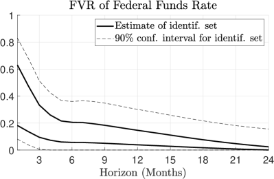
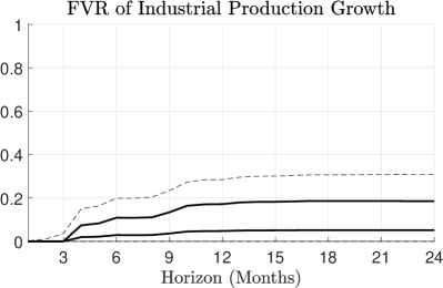
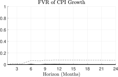
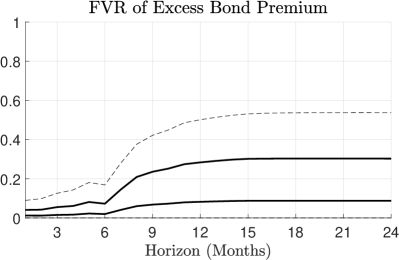
Figure 1: Point estimates and 90% confidence intervals for the identified sets of forecast variance ratios, across different variables and forecast horizons. For visual clarity, we force bias-corrected estimates/bounds to lie in $[0,1]$. The interest rate variable is the Federal Funds Rate.

Figure 1 shows partial identification robust confidence intervals for the forecast variance ratio of the four endogenous macro variables with respect to the monetary shock. We report point estimates and confidence intervals for the identified sets at each horizon separately. We focus here on the specification with the FFR instead of the 1-year rate, since our quantitative conclusions are if anything even starker with the latter observable. At all forecast horizons, the 90% confidence intervals rule out FVRs above 31% for output growth and 8% for inflation. At forecast horizons up to 6 months, we can rule out that the monetary shock accounts for more than 19% of the forecast variance of the Excess Bond Premium. However, we cannot rule out that the monetary shock is an important contributor to medium- or long-run forecasts of the bond premium. On the other hand, we cannot rule out that the monetary shock is completely unimportant either.

Our analysis reveals that the weak assumptions of the SVMA-IV model suffice to obtain tight upper bounds on the forecast variance contribution of monetary shocks for several variables, especially inflation. This is despite the finding by Stock & Watson (2018) that standard errors for impulse response functions are large in this application. Many commentators have documented a recent divorce between inflation and output dynamics (Hall, 2011); our results document a similar divorce in dynamics conditional on monetary policy shocks in post-1990 data. Although this finding echoes previous SVAR work (Christiano et al., 1999; Ramey, 2016), our identifying assumptions are weaker – we merely impose validity of the IV. We conclude that, if inflation is a monetary phenomenon, it is so because of the systematic component of monetary policy, not because of erratic policy shocks.

Other application: Oil news shocks.

In LABEL:sec:oil we show that our method also yields highly informative upper bounds on the importance of international oil supply news shocks for the U.S. and global business cycles. We use an IV constructed by Känzig (2021) from OPEC announcements. We find the oil news shock to be highly non-invertible, causing conventional SVAR-IV analysis to reach several spurious conclusions.

6 Analytical illustrations

In this section we consider three simple analytical examples that illustrate how our identification bounds depend on the characteristics of the data. Section 3.2 argued that the tightness of our lower bound on variance decompositions depends solely on the strength of the IV. We here show that, under stylized but empirically motivated assumptions, the upper bound can be expected to be highly informative, in the sense that it at worst mildly overstates the instrumented shock’s contribution to macroeconomic fluctuations.

Throughout this section we assume the availability of a single IV $z_{t}=\alpha\varepsilon_{1,t}+\sigma_{v}v_{t}$, and then consider different illustrative toy models for the $y_{t}$ variables, as specified below. In LABEL:sec:sw_illustration we extend the analytical intuition below to the much richer quantitative DSGE model developed by Smets & Wouters (2007).

6.1 Information content of several observables

As our first example, consider the static model

$$y_{t}=\Theta_{0}\varepsilon_{t}$$

with $n_{y}=2$ observables: inflation ($y_{1,t}$) and the monetary policy interest rate ($y_{2,t}$). We think of $\varepsilon_{1,t}$ as a conventional monetary policy shock. If we only observed inflation $y_{1,t}$ in addition to an IV, we would not be able to rule out that the monetary shock drives all the variation in this single variable, as explained in Section 3.1. How can adding the interest rate to the data set help tighten the identified set for the FVR of inflation?

To gain economic intuition, let the reduced-form moments of the data be given by

$$\operatorname*{Var}(y_{t})=\left(\begin{smallmatrix}1&\rho\\ \rho&1\end{smallmatrix}\right),\quad\text{and}\quad\operatorname*{Cov}(y_{t},z_{t})=\left(\begin{smallmatrix}1\\ -\zeta\end{smallmatrix}\right),$$

where $\zeta\geq 0$. We see that, even with the amount of measurement error unknown, the IV $z_{t}$ reveals the signs and the relative magnitudes of the co-movement in observables induced by monetary shocks: The shock $\varepsilon_{1,t}$ moves inflation and interest rates in opposite directions (Uhlig, 2005), while the unconditional correlation of interest rates and inflation is $\rho$.

We consider three instructive special cases. For the first two, we set $\zeta=1$; applying our identification analysis, we then get the bounds

$$\mathit{FVR}_{i,0}\leq\frac{1}{2}(1-\rho),\quad i=1,2.$$

Now suppose first that $\rho=-1$; that is, interest rates and inflation are not just perfectly negatively correlated conditional on monetary shocks, but also unconditionally. In that case the upper bound for the FVR of both variables equals 1: The data cannot rule out that the correlation of the IV with macro observables is imperfect purely because of measurement error. Second, suppose that $\rho=1$; that is, interest rates and inflation are perfectly positively correlated in the data. Then our upper bound for the FVR suddenly equals zero: The monetary shock induces co-movement patterns that we never see in the data, so it cannot possibly explain any observed macro fluctuations. Third, if instead $\rho=0$, then our upper bounds are, for any $\zeta\geq 0$,

$$\mathit{FVR}_{1,0}\leq\frac{1}{1+\zeta^{2}},\quad\mathit{FVR}_{2,0}\leq\frac{\zeta^{2}}{1+\zeta^{2}}.$$

Suppose that nominal rates respond much more to the monetary shock than inflation does, i.e., $\zeta\gg 1$. Then the upper bound on the inflation variance decomposition $\mathit{FVR}_{1,0}$ is very small; intuitively, since the IV reveals that the monetary shock moves interest rates by much more than inflation, but both have the same unconditional variance, the monetary shock cannot possibly be an important driver of inflation. This third example rationalizes the findings in our application to monetary shocks in Section 5: The IV $z_{t}$ correlates much more with interest rates than with prices, yet prices are not commensurately less volatile than interest rates, so monetary shocks cannot account for much of the volatility in prices.

This example shows that our upper bound on the FVR is close to the true value if either the shock is very prominent (so that the bound of one is not far from the truth) or if the shock induces somehow atypical co-movements of the various observed macro aggregates. This second condition is equivalent to the shock being prominent for some linear combination of the macro observables $y_{t}$, which is equivalent to the shock being nearly invertible in this static model. Thus, the preceding arguments agree with the analysis in Section 3.1.

6.2 Dynamic information content

Whereas the previous example illustrated how the availability of several macro time series sharpens identification in a static context, we now show how the dynamics of individual time series can do the same. Consider the univariate but dynamic model

$$y_{t}=\sum_{j=1}^{n_{\varepsilon}}\sum_{\ell=0}^{\infty}\rho_{j}^{\ell}\varepsilon_{j,t-\ell}$$

with $n_{y}=1$. That is, we observe a single variable $y_{t}$ driven by $n_{\varepsilon}$ independent AR(1) processes. To fix ideas, we think of $\varepsilon_{1,t}$ as a technology shock and $y_{t}$ as aggregate output.

Now assume that long-run fluctuations in output $y_{t}$ are exclusively driven by the technology shock $\varepsilon_{1,t}$; that is, consider the limit $\rho_{1}\rightarrow 1$, while fixing $|\rho_{j}|<1$ for all $j\geq 2$. In this case, the sharp lower bound on $\alpha^{2}$ converges to the truth:

$$\lim_{\rho_{1}\to 1}\alpha_{LB}^{2}=\lim_{\rho_{1}\to 1}2\pi\sup_{\omega\in[0,\pi]}s_{\tilde{z}^{\dagger}}(\omega)=\lim_{\rho_{1}\to 1}2\pi s_{\tilde{z}^{\dagger}}(0)=\alpha^{2}.$$

Intuitively, at spectral frequency zero, all fluctuations in $y_{t}$ are driven by the technology shock. Loosely speaking, applying a low-pass filter to $y_{t}$ therefore isolates the fluctuations caused by the technology shock. Leads and lags of this low-pass filtered series are thus highly correlated with the IV, putting a lower bound on the signal-to-noise ratio in the IV. This is why the sharp upper bound for the FVR converges to the true value.

The example reveals that cross-restrictions over time can be highly informative even if the shock of interest is neither invertible nor recoverable. Intuitively, for the sharp upper bound on the FVR to bind, our method only needs the shock to dominate at some frequency; the across-frequency restrictions then do the rest, exactly like the cross-variable restrictions in the static example above.

6.3 Non-invertibility and news shocks

In the third example, we show how our method deals with non-invertible news shocks. First discussed in Pigou (1927), news shocks have recently received much attention as drivers of macroeconomic fluctuations (Beaudry & Portier, 2006, 2014; Jaimovich & Rebelo, 2009; Schmitt-Grohé & Uribe, 2012). Unfortunately, foresight of economic agents complicates conventional SVAR-based analysis since it induces equilibria with non-invertible MA representations (Leeper et al., 2013). In contrast, our methods are valid irrespective of invertibility.

To illustrate, consider a moving average model of order 1 with $n_{y}=n_{\varepsilon}=2$:

$$y_{t}=(1+\zeta L)\Theta_{0}\varepsilon_{t},$$

where $\zeta>1$. As is well known, this assumption implies that the moving average representation is non-invertible. We think of $\varepsilon_{1,t}$ as a monetary forward guidance shock: The shock moves inflation and nominal interest rates by more tomorrow (when the shock directly hits the monetary policy rule) than today (when the news is revealed).

The conventional SVAR-IV approach mis-measures the FVR because of non-invertibility. By standard arguments (e.g., Leeper et al., 2013) the reduced-form VAR residuals equal

$$u_{t}\equiv y_{t}-E(y_{t}\mid\{y_{\tau}\}_{-\infty<\tau<t})=\Theta_{0}\varepsilon_{t}+(1-1/R_{0}^{2})\sum_{\ell=1}^{\infty}\left(-\zeta\right)^{-\ell}\Theta_{0}\varepsilon_{t-\ell},$$ (21)

where the degree of invertibility equals

$$R_{0}^{2}=\zeta^{-2}.$$

Since SVAR procedures assume that the structural shocks $\varepsilon_{t}$ can be obtained as linear functions of the reduced-form residuals $u_{t}$, equation (21) shows that any SVAR analysis will conflate the explanatory power of the shock $\varepsilon_{1,t}$ with that of its lags. As a consequence, LABEL:sec:svar_iv shows that the SVAR-IV estimand of the FVR overstates the contribution of the shock to one-step-ahead forecasts:

$$\mathit{FVR}_{1,0}^{\mathit{SVAR-IV}}=\frac{1}{R_{0}^{2}}\times\mathit{FVR}_{1,0}>\mathit{FVR}_{1,0}.$$

Clearly, the population bias of the SVAR-IV estimand worsens as the degree of invertibility $R_{0}^{2}$ decreases to 0 (see also Forni et al., 2019). In the oil news shock application in LABEL:sec:oil we demonstrate that the SVAR-IV bias can be large in practice.

In contrast, our identification bounds are valid irrespective of invertibility, since we do not assume that $\varepsilon_{1,t}$ can be recovered as a function of only the contemporaneous VAR residuals $u_{t}$. In fact, in this model with as many observables as shocks, both shocks $\varepsilon_{t}=(\varepsilon_{1,t},\varepsilon_{2,t})^{\prime}$ are recoverable. Hence, if we exploit this knowledge, we can even point-identify the shock as $\varepsilon_{1,t}\propto z_{t}^{\dagger}=E(z_{t}\mid\{y_{\tau}\}_{-\infty<\tau<\infty})$. The key is that our method can use the future values of nominal rates and inflation, $y_{\tau}$, $\tau\geq t$, to recover the forward guidance shock $\varepsilon_{1,t}$ at time $t$. In so doing, it effectively realigns the information sets of the economic agents and of the econometrician, sidestepping the invertibility problem.

7 Simulation study

We finish by showing that our inference procedures have good finite-sample performance in simulations. Our methods continue to work well in non-invertible models, unlike the conventional SVAR-IV procedure.

DGP.

We adopt a variant of the DGP in Kilian & Kim (2011) and assume that the macro aggregates $y_{t}$ follow a structural VARMA($p$,1) model:

$$y_{t}=\textstyle\sum_{\ell=1}^{p}\Xi_{\ell}y_{t-\ell}+\Theta_{0}(\varepsilon_{t}+\zeta\varepsilon_{t-1}).$$

We consider $n_{y}=2$ macro variables, $p=1$ autoregressive lag (with one exception discussed below), and set $\Xi_{1}=\left(\begin{smallmatrix}\rho_{y}&0\\ 0.5&0.5\end{smallmatrix}\right)$. For the MA part, we consider $n_{\varepsilon}=2$ shocks (which are thus both recoverable) and set $\Theta_{0}=\text{chol}\left(\begin{smallmatrix}1&0.8\\ 0.8&1\end{smallmatrix}\right),$ where “chol” denotes the lower triangular Cholesky decomposition. As in Section 6.3, $\zeta$ is a scalar parameter that governs the degree of invertibility, with $\zeta>1$ implying non-invertibility. We add an external instrument $z_{t}$ for the shock of interest $\varepsilon_{1,t}$:

$$z_{t}=\rho_{z}z_{t-1}+\rho_{zy}(y_{1,t-1}+y_{2,t-1})+\varepsilon_{1,t}+\sigma_{v}v_{t}.$$

Notice that we have normalized $\alpha=1$. Finally, the measurement error and structural shocks are i.i.d. Gaussian and orthogonal as in Assumption 3.

We run Monte Carlo experiments for nine different parameterizations of the above DGP. Specifically, we consider various deviations from a baseline parametrization. In our benchmark, we set $\rho_{y}=0.5$, $\rho_{z}=\rho_{zy}=0$, $\zeta=0$, $\sigma_{v}=1$, and sample size $T=250$. We then consider variations with more autoregressive persistence (either $\rho_{y}=0.9$, or $\rho_{z}=0.8$ and $\rho_{zy}=0.3$), an invertible MA component ($\zeta=0.5$), a non-invertible MA component ($\zeta=2$), a weaker instrument ($\sigma_{v}=2$), and different sample sizes ($T=100$, $T=500$). Finally, we allow for richer dynamics, with $p=4$ and $\Xi_{j}=\frac{1}{j^{2}}\Xi_{1}$ for $j=2,3,4$.

Results.

Our parameters of interest are the degree of invertibility $R_{0}^{2}$ and the FVR for variable $y_{2,t}$ at horizons $1$ and $4$. We conduct $5,000$ Monte Carlo repetitions per DGP, and construct confidence intervals at the 90% level using $1,000$ bootstrap draws per simulation. We use a homoskedastic recursive residual bootstrap. The reduced-form VAR lag length is selected using AIC, and we use Hall’s percentile bootstrap confidence interval, cf. Section 4.

Monte Carlo study: Coverage rates of confidence intervals
True parameter Coverage $R_{0}^{2}$ Coverage $\mathit{FVR}_{2,1}$ Coverage $\mathit{FVR}_{2,4}$ Experiment $R_{0}^{2}$ $\mathit{FVR}_{2,1}$ $\mathit{FVR}_{2,4}$ Set Param Set Param SVAR Set Param SVAR Baseline 1 0.64 0.819 0.935 0.999 0.898 0.955 0.867 0.880 0.948 0.838 $\rho_{y}=0.9$ 1 0.64 0.862 0.929 1.000 0.896 0.953 0.876 0.889 0.952 0.824 $\rho_{z}=0.8$, $\rho_{zy}=0.3$ 1 0.64 0.819 0.933 1.000 0.904 0.960 0.873 0.891 0.959 0.850 $\zeta=0.5$ 1 0.64 0.839 0.937 0.998 0.892 0.944 0.870 0.853 0.928 0.828 $\zeta=2$ 0.25 0.16 0.806 0.879 0.910 0.857 0.881 0.137 0.861 0.938 0.674 $\sigma_{v}=2$ 1 0.64 0.819 0.949 0.997 0.889 0.924 0.824 0.865 0.903 0.770 $T=100$ 1 0.64 0.819 0.907 0.998 0.871 0.943 0.835 0.840 0.929 0.797 $T=500$ 1 0.64 0.819 0.931 1.000 0.900 0.954 0.881 0.884 0.947 0.869 $p=4$ 1 0.64 0.855 0.937 0.999 0.897 0.945 0.868 0.829 0.868 0.846

Table 2: True parameter values and coverage rates of 90% confidence intervals, constructed as in Section 4, using 1,000 bootstrap iterations for each Monte Carlo experiment, and 5,000 Monte Carlo experiments per DGP. The DGPs (along rows) are described in the text. “Set”: probability that SVMA-IV confidence interval covers entire identified set. “Param”: probability that SVMA-IV confidence interval covers parameter. “SVAR”: probability that conventional SVAR-IV confidence interval covers parameter.

Table 2 shows that the partial identification robust SVMA-IV confidence sets defined in Section 4 achieve coverage rates close to or exceeding the desired level of 90% throughout. We report coverage rates for both the population identified sets (columns “Set”) and for the underlying parameters (columns “Param”). The coverage rate for the parameter is never below 86.8% in any case. The coverage rate for the identified set is mostly close to 90% and at worst 82.9% in our experiments. We also report the coverage rates of conventional SVAR-IV bootstrap confidence intervals for the FVR (columns “SVAR”). The coverage distortions of our SVMA-IV procedures are almost always smaller than those of the SVAR-IV procedure. Most notably, our procedures have acceptable coverage even in the non-invertible case ($\zeta=2$), whereas the SVAR-IV procedure under-covers severely in this case.

We make the following additional remarks. First, coverage deteriorates slightly with noisier/weaker instruments ($\sigma_{v}=2$), as expected. Our inference methods are not robust to arbitrarily weak instruments ($\sigma_{v}\to\infty$); we leave this issue to future work. Second, we face some well-known parameter-at-the-boundary issues. For most experiments, $R_{0}^{2}=1$. This explains the over-coverage of confidence intervals for this parameter and, less so, for the overall identified set. Similar problems would arise if the true FVR were close to $0$. Third, for more persistent DGPs, the AIC tends to select an insufficient number of lags, resulting in moderate under-coverage, in particular for the FVRs at horizon 4. For example, in the experiment with $p=4$ autoregressive lags, the AIC selects an average lag length of $2.2$.

8 Conclusion

Applied macroeconomists have recently turned to external sources of exogenous variation to identify dynamic causal effects. Though such external instruments or proxies are frequently used to estimate impulse responses, existing methods did not allow researchers to quantify the contribution of individual shocks to business-cycle fluctuations – a question of first-order interest in traditional business-cycle analysis. We fill this gap by providing identification results and inference techniques for variance decompositions, historical decompositions, and the degree of invertibility. Our methods require neither the absence of measurement error in the external instrument, nor the often dubious assumption that the instrumented shock is invertible (as assumed in conventional SVAR analysis). We prove that the importance of the instrumented shock is generally interval-identified. Point identification can be achieved if the shock is known to be recoverable – a substantively weaker assumption than invertibility. We provide a software package that implements all steps of our inference procedures. Applying our method to U.S. data, we are able to establish a tight upper bound on the importance of monetary shocks for recent inflation dynamics, despite our weak identifying assumptions.

Appendix A Appendix

A.1 Formulas for estimation and inference

Here we provide the remaining formulas needed for the inference procedures in Section 4.

Let $\hat{A}_{1},\dots,\hat{A}_{p}$ denote the $(n_{y}+1)\times(n_{y}+1)$ coefficient matrix estimates for the VAR in $W_{t}=(y_{t}^{\prime},z_{t})^{\prime}$. Let $\hat{\Sigma}$ denote the residual sample variance-covariance matrix. Let $\hat{\Sigma}^{1/2}$ denote any square matrix such that $\hat{\Sigma}^{1/2}\hat{\Sigma}^{1/2\prime}=\hat{\Sigma}$, e.g., the Cholesky factor. Compute the moving average coefficients $\hat{B}(L)\equiv(I_{n_{y}+1}-\sum_{\ell=1}^{p}\hat{A}_{\ell}L^{\ell})^{-1}\hat{\Sigma}^{1/2}$ using the familiar recursion

$$\hat{B}_{0}=\hat{\Sigma}^{1/2},\quad\hat{B}_{h}=\textstyle\sum_{\ell=1}^{\min\{h,p\}}\hat{A}_{\ell}\hat{B}_{h-\ell},\;h\geq 1.$$

Denote the top $n_{y}$ rows of $\hat{B}_{h}$ by $\hat{B}_{y,h}$ and the bottom row by $\hat{B}_{z,h}$. Then

$$\widehat{\operatorname*{Var}}(\tilde{z}_{t})\equiv\hat{B}_{z,0}\hat{B}_{z,0}^{\prime},\quad\widehat{\operatorname*{Cov}}(\tilde{z}_{t},y_{t+h})\equiv\begin{cases}\hat{B}_{z,0}\hat{B}_{y,h}^{\prime}&\text{if $h\geq 0$},\\ 0_{1\times n_{y}}&\text{otherwise},\end{cases}$$

$$\widehat{\operatorname*{Cov}}(y_{t},y_{t-h})\equiv\textstyle\sum_{\ell=0}^{\infty}\hat{B}_{y,\ell}\hat{B}_{y,\ell+h}^{\prime}\text{ for }h\geq 0.$$

In practice, we truncate the infinite sum above at a large value of $\ell$.

Define now the projection variances

$$\widehat{\operatorname*{Var}}(E(\tilde{z}_{t}\mid\{y_{\tau}\}_{-\infty<\tau<\infty})) \equiv\hat{\Sigma}_{\tilde{z},y,(M,M)}\hat{\Sigma}_{y,(M,M)}^{-1}\hat{\Sigma}_{\tilde{z},y,(M,M)}^{\prime},$$

$$\widehat{\operatorname*{Var}}(y_{i,t+\ell}\mid\{y_{\tau}\}_{-\infty<\tau\leq t}) \equiv\widehat{\operatorname*{Var}}(y_{i,t})-(\widehat{\operatorname*{Cov}}(y_{i,t+\ell},y_{t}),\dots,\widehat{\operatorname*{Cov}}(y_{i,t+\ell},y_{t-M}))\widehat{\Sigma}_{y,(M,0)}^{-1}$$

$$\qquad\qquad\qquad\times(\widehat{\operatorname*{Cov}}(y_{i,t+\ell},y_{t}),\dots,\widehat{\operatorname*{Cov}}(y_{i,t+\ell},y_{t-M}))^{\prime},$$

$$\widehat{\operatorname*{Var}}(E(\tilde{z}_{t}\mid\{y_{\tau}\}_{-\infty<\tau\leq t})) \equiv(\widehat{\operatorname*{Cov}}(\tilde{z}_{t},y_{t}),0_{1\times n_{y}M})\hat{\Sigma}_{y,(M,0)}^{-1}(\widehat{\operatorname*{Cov}}(\tilde{z}_{t},y_{t}),0_{1\times n_{y}M})^{\prime},$$

where $\hat{\Sigma}_{\tilde{z},y,(M,M)}$ is the estimated covariance vector of $\tilde{z}_{t}$ and $(y_{t+M}^{\prime},\dots,y_{t}^{\prime},\dots,y_{t-M}^{\prime})^{\prime}$ obtained by stacking the estimates $\widehat{\operatorname*{Cov}}(\tilde{z}_{t},y_{t+h})$ defined above, $\hat{\Sigma}_{y,(M,M)}$ is similarly the estimated variance-covariance matrix of $(y_{t+M}^{\prime},\dots,y_{t}^{\prime},\dots,y_{t-M}^{\prime})^{\prime}$, and $\hat{\Sigma}_{y,(M,0)}$ is the estimated variance-covariance matrix of $(y_{t}^{\prime},y_{t-1}^{\prime},\dots,y_{t-M}^{\prime})^{\prime}$.

In these formulas, the integer $M$ is a numerical truncation parameter. For example, we estimate $\operatorname*{Var}(E(\tilde{z}_{t}\mid\{y_{\tau}\}_{-\infty<\tau<\infty}))$ using an estimate of the truncated conditional variance $\operatorname*{Var}(E(\tilde{z}_{t}\mid\{y_{\tau}\}_{t-M\leq\tau\leq t+M}))$. $M$ should exceed at least 50 to yield an accurate approximation. We recommend checking that the numerical results do not change much when $M$ is increased, since the effects of truncation will depend on the persistence of the data.

A.2 Proofs of main results

A.2.1 Auxiliary lemma

Lemma 1.

Let $B$ be an $n\times n$ Hermitian positive definite complex-valued matrix and $b$ an $n$-dimensional complex-valued column vector. Let $x$ be a nonnegative real scalar. Then $B-x^{-1}bb^{*}$ is positive (semi)definite if and only if $x>\!(\geq)\,b^{*}B^{-1}b$.

Please find the proof in LABEL:sec:proof_semidef.

A.2.2 Proof of Proposition 1

Let $\alpha$ and the spectrum $s_{w}(\omega)$ be given. Define the $n_{y}$-dimensional vectors

$$\overline{\Theta}_{\bullet,1,\ell}=\alpha^{-1}\operatorname*{Cov}(y_{t},\tilde{z}_{t-\ell}),\quad\ell\geq 0,$$

and the corresponding vector lag polynomial

$$\overline{\Theta}_{\bullet,1}(L)=\sum_{\ell=0}^{\infty}\overline{\Theta}_{\bullet,1,\ell}L^{\ell}.$$

Since $\alpha^{2}\leq\alpha_{UB}^{2}$, we may define $\overline{\sigma}_{v}=\sqrt{\operatorname*{Var}(\tilde{z}_{t})-\alpha^{2}}$. Since $\alpha^{2}>\alpha_{LB}^{2}$, Lemma 1 implies that

$$s_{y}(\omega)-\frac{2\pi}{\alpha^{2}}s_{y\tilde{z}}(\omega)s_{y\tilde{z}}(\omega)^{*}=s_{y}(\omega)-\frac{1}{2\pi}\overline{\Theta}_{\bullet,1}(e^{-i\omega})\overline{\Theta}_{\bullet,1}(e^{-i\omega})^{*}$$

is positive definite for every $\omega\in[0,2\pi]$. Hence, the Wold decomposition theorem (Hannan, 1970, Thm. $2^{\prime\prime}$, p. 158) implies that there exists an $n_{y}\times n_{y}$ matrix lag polynomial $\tilde{\Theta}(L)=\sum_{\ell=0}^{\infty}\tilde{\Theta}_{\ell}L^{\ell}$ such that

$$s_{y}(\omega)-\frac{1}{2\pi}\overline{\Theta}_{\bullet,1}(e^{-i\omega})\overline{\Theta}_{\bullet,1}(e^{-i\omega})^{*}=\frac{1}{2\pi}\tilde{\Theta}(e^{-i\omega})\tilde{\Theta}(e^{-i\omega})^{*},\quad\omega\in[0,2\pi].$$

Thus, the following model for $w_{t}=(y_{t}^{\prime},\tilde{z}_{t})^{\prime}$ generates the desired spectrum $s_{w}(\omega)$:

$$y_{t} =\overline{\Theta}_{\bullet,1}(L)\overline{\varepsilon}_{1,t}+\tilde{\Theta}(L)\tilde{\varepsilon}_{t},$$

$$\tilde{z}_{t} =\alpha\overline{\varepsilon}_{1,t}+\overline{\sigma}_{v}\overline{v}_{t},$$

$$(\overline{\varepsilon}_{1,t},\tilde{\varepsilon}_{t}^{\prime},\overline{v}_{t})^{\prime} \stackrel{{\scriptstyle i.i.d.}}{{\sim}}N(0,I_{n_{y}+2}).$$

Note that the construction requires only $n_{\varepsilon}=n_{y}+1$ shocks, $\overline{\varepsilon}_{1,t}\in\mathbb{R}$ and $\tilde{\varepsilon}_{t}\in\mathbb{R}^{n_{y}}$. ∎

A.2.3 Proof of Proposition 2

Identified set for $R_{0}^{2}$.

If the identified set contains 1, then there must exist an $\overline{\alpha}\in[\alpha_{LB},\alpha_{UB}]$ and i.i.d., independent standard Gaussian processes $\overline{\varepsilon}_{1,t}$ and $\overline{v}_{t}$ such that (i) $\tilde{z}_{t}=\overline{\alpha}\times\overline{\varepsilon}_{1,t}+\overline{v}_{t}$, (ii) $\overline{v}_{t}$ is uncorrelated with $y_{t}$ at all leads and lags, and (iii) $\overline{\varepsilon}_{1,t}$ lies in the closed linear span of $\{y_{\tau}\}_{-\infty<\tau\leq t}$. This immediately implies the “only if” statement.

For the “if” part, assume $\tilde{z}_{t}$ does not Granger cause $y_{t}$. By the equivalence of Sims and Granger causality, $\tilde{z}_{t}^{\dagger}=E(\tilde{z}_{t}\mid\{y_{\tau}\}_{-\infty<\tau<\infty})=E(\tilde{z}_{t}\mid\{y_{\tau}\}_{-\infty<\tau\leq t})$. Note that the latter best linear predictor is white noise since, for any $\ell\geq 1$,

$$\operatorname*{Cov}\big{(}E(\tilde{z}_{t}\mid\{y_{\tau}\}_{-\infty<\tau\leq t}),y_{t-\ell}\big{)} =\operatorname*{Cov}(\tilde{z}_{t},y_{t-\ell})-\operatorname*{Cov}\big{(}\tilde{z}_{t}-E(\tilde{z}_{t}\mid\{y_{\tau}\}_{-\infty<\tau\leq t}),y_{t-\ell}\big{)}$$

$$=0-0,$$

using the fact that $\tilde{z}_{t}$ is a projection residual. In conclusion, the best linear predictor $\tilde{z}_{t}^{\dagger}$ of $\tilde{z}_{t}$ given $\{y_{\tau}\}_{-\infty<\tau<\infty}$ depends only on $\{y_{\tau}\}_{-\infty<\tau\leq t}$ and it has a constant spectrum. From the expression for $\alpha_{LB}^{2}$, we get that $\alpha_{LB}^{2}=\operatorname*{Var}(E(\tilde{z}_{t}\mid\{y_{\tau}\}_{-\infty<\tau\leq t}))$. Hence, expression (17) implies that the upper bound of the identified set for $R_{0}^{2}$ equals 1.

Identified set for $R_{\infty}^{2}$.

The upper bound of the identified set for $R_{\infty}^{2}$ equals 1 if and only if $2\pi\sup_{\omega\in[0,\pi]}s_{\tilde{z}^{\dagger}}(\omega)=\operatorname*{Var}(E(\tilde{z}_{t}\mid\{y_{\tau}\}_{-\infty<\tau<\infty}))$. The right-hand side of this equation equals $\operatorname*{Var}(\tilde{z}_{t}^{\dagger})=\int_{0}^{2\pi}s_{\tilde{z}^{\dagger}}(\omega)\,d\omega$. But $\sup_{\omega\in[0,\pi]}s_{\tilde{z}^{\dagger}}(\omega)=\frac{1}{2\pi}\int_{0}^{2\pi}s_{\tilde{z}^{\dagger}}(\omega)\,d\omega$ if and only if $s_{\tilde{z}^{\dagger}}(\omega)$ is constant in $\omega$ almost everywhere, i.e., $\tilde{z}_{t}^{\dagger}$ is white noise. ∎

References

- Andrews & Shi (2013) Andrews, D. W. & Shi, X. (2013). Inference Based on Conditional Moment Inequalities. Econometrica, 81(2), 609–666.
- Andrews & Shi (2017) Andrews, D. W. & Shi, X. (2017). Inference based on many conditional moment inequalities. Journal of Econometrics, 196(2), 275–287.
- Beaudry & Portier (2006) Beaudry, P. & Portier, F. (2006). Stock Prices, News, and Economic Fluctuations. American Economic Review, 96(4), 1293–1307.
- Beaudry & Portier (2014) Beaudry, P. & Portier, F. (2014). News-Driven Business Cycles: Insights and Challenges. Journal of Economic Literature, 52(4), 993–1074.
- Blanchard et al. (2013) Blanchard, O. J., L’Huillier, J. P., & Lorenzoni, G. (2013). News, Noise, and Fluctuations: An Empirical Exploration. American Economic Review, 103(7), 3045–3070.
- Brockwell & Davis (1991) Brockwell, P. J. & Davis, R. A. (1991). Time Series: Theory and Methods (2nd ed.). Springer Series in Statistics. Springer.
- Caldara & Herbst (2019) Caldara, D. & Herbst, E. (2019). Monetary policy, real activity, and credit spreads: Evidence from bayesian proxy svars. American Economic Journal: Macroeconomics, 11(1), 157–92.
- Campbell et al. (2012) Campbell, J. R., Evans, C. L., Fisher, J. D. M., & Justiniano, A. (2012). Macroeconomic Effects of Federal Reserve Forward Guidance. Brookings Papers on Economic Activity, 2012(Spring), 1–80.
- Chahrour & Jurado (2021) Chahrour, R. & Jurado, K. (2021). Recoverability and Expectations-Driven Fluctuations. Review of Economic Studies. Forthcoming.
- Chernozhukov et al. (2013) Chernozhukov, V., Lee, S., & Rosen, A. M. (2013). Intersection Bounds: Estimation and Inference. Econometrica, 81(2), 667–737.
- Christiano et al. (1999) Christiano, L., Eichenbaum, M., & Evans, C. (1999). Monetary Policy Shocks: What Have We Learned and to What End? In J. B. Taylor & M. Woodford (Eds.), Handbook of Macroeconomics, Volume 1A chapter 2, (pp. 65–148). Elsevier.
- Cochrane & Piazzesi (2002) Cochrane, J. H. & Piazzesi, M. (2002). The Fed and Interest Rates—A High-Frequency Identification. American Economic Review, 92(2), 90–95.
- Forni & Gambetti (2014) Forni, M. & Gambetti, L. (2014). Sufficient information in structural VARs. Journal of Monetary Economics, 66(Supplement C), 124–136.
- Forni et al. (2017a) Forni, M., Gambetti, L., Lippi, M., & Sala, L. (2017a). Noise Bubbles. Economic Journal, 127(604), 1940–1976.
- Forni et al. (2017b) Forni, M., Gambetti, L., Lippi, M., & Sala, L. (2017b). Noisy News in Business Cycles. American Economic Journal: Macroeconomics, 9(4), 122–152.
- Forni et al. (2019) Forni, M., Gambetti, L., & Sala, L. (2019). Structural VARs and noninvertible macroeconomic models. Journal of Applied Econometrics, 34(2), 221–246.
- Gafarov et al. (2018) Gafarov, B., Meier, M., & Montiel Olea, J. L. (2018). Delta-Method Inference for a Class of Set-Identified SVARs. Journal of Econometrics, 203(2), 316–327.
- Gertler & Karadi (2015) Gertler, M. & Karadi, P. (2015). Monetary Policy Surprises, Credit Costs, and Economic Activity. American Economic Journal: Macroeconomics, 7(1), 44–76.
- Giannone & Reichlin (2006) Giannone, D. & Reichlin, L. (2006). Does Information Help Recovering Structural Shocks from Past Observations? Journal of the European Economic Association, 4(2/3), 455–465.
- Gilchrist & Zakrajšek (2012) Gilchrist, S. & Zakrajšek, E. (2012). Credit Spreads and Business Cycle Fluctuations. American Economic Review, 102(4), 1692–1720.
- Gorodnichenko & Lee (2020) Gorodnichenko, Y. & Lee, B. (2020). Forecast Error Variance Decompositions with Local Projections. Journal of Business & Economic Statistics, 38(4), 921–933.
- Gürkaynak et al. (2005) Gürkaynak, R. S., Sack, B. P., & Swanson, E. T. (2005). Do Actions Speak Louder Than Words? The Response of Asset Prices to Monetary Policy Actions and Statements. The International Journal of Central Banking, 1(1), 55–93.
- Hall (2011) Hall, R. E. (2011). The Long Slump. American Economic Review, 101(2), 431–469.
- Hannan (1970) Hannan, E. (1970). Multiple Time Series. Wiley Series in Probability and Statistics. John Wiley & Sons.
- Imbens & Manski (2004) Imbens, G. W. & Manski, C. F. (2004). Confidence Intervals for Partially Identified Parameters. Econometrica, 72(6), 1845–1857.
- Jaimovich & Rebelo (2009) Jaimovich, N. & Rebelo, S. (2009). Can News about the Future Drive the Business Cycle? American Economic Review, 99(4), 1097–1118.
- Jordà (2005) Jordà, Ò. (2005). Estimation and Inference of Impulse Responses by Local Projections. American Economic Review, 95(1), 161–182.
- Känzig (2021) Känzig, D. R. (2021). The Macroeconomic Effects of Oil Supply News: Evidence from OPEC Announcements. American Economic Review, 111(4), 1092–1125.
- Kilian & Kim (2011) Kilian, L. & Kim, Y. J. (2011). How Reliable Are Local Projection Estimators of Impulse Responses? Review of Economics and Statistics, 93(4), 1460–1466.
- Kilian & Lütkepohl (2017) Kilian, L. & Lütkepohl, H. (2017). Structural Vector Autoregressive Analysis. Cambridge University Press.
- Klepper & Leamer (1984) Klepper, S. & Leamer, E. E. (1984). Consistent Sets of Estimates for Regressions with Errors in All Variables. Econometrica, 52(1), 163–183.
- Kuttner (2001) Kuttner, K. (2001). Monetary Policy Surprises and Interest Rates: Evidence from the Fed Funds Futures Market. Journal of Monetary Economics, 47(3), 523–544.
- Leeper et al. (2013) Leeper, E. M., Walker, T. B., & Yang, S.-C. S. (2013). Fiscal Foresight and Information Flows. Econometrica, 81(3), 1115–1145.
- Lippi & Reichlin (1994) Lippi, M. & Reichlin, L. (1994). VAR analysis, nonfundamental representations, Blaschke matrices. Journal of Econometrics, 63(1), 307–325.
- Mertens (2015) Mertens, K. (2015). Advances in Empirical Macroeconomics, Lecture 2. Lecture slides, Bonn Summer School.
- Mertens & Ravn (2010) Mertens, K. & Ravn, M. O. (2010). Measuring the Impact of Fiscal Policy in the Face of Anticipation: A Structural VAR Approach. Economic Journal, 120(544), 393–413.
- Mertens & Ravn (2013) Mertens, K. & Ravn, M. O. (2013). The Dynamic Effects of Personal and Corporate Income Tax Changes in the United States. American Economic Review, 103(4), 1212–1247.
- Nakamura & Steinsson (2018a) Nakamura, E. & Steinsson, J. (2018a). High Frequency Identification of Monetary Non-Neutrality: The Information Effect. Quarterly Journal of Economics, 133(3), 1283–1330.
- Nakamura & Steinsson (2018b) Nakamura, E. & Steinsson, J. (2018b). Identification in Macroeconomics. Journal of Economic Perspectives, 32(3), 59–86.
- Pigou (1927) Pigou, A. C. (1927). Industrial Fluctuations (2 ed.). London: Macmillan.
- Plagborg-Møller (2019) Plagborg-Møller, M. (2019). Bayesian inference on structural impulse response functions. Quantitative Economics, 10(1), 145–184.