Detecting direct causality in multivariate time series: A comparative study

Abstract

The concept of Granger causality is increasingly being applied for the characterization of directional interactions in different applications. A multivariate framework for estimating Granger causality is essential in order to account for all the available information from multivariate time series. However, the inclusion of non-informative or non-significant variables creates estimation problems related to the ’curse of dimensionality’. To deal with this issue, direct causality measures using variable selection and dimension reduction techniques have been introduced. In this comparative work, the performance of an ensemble of bivariate and multivariate causality measures in the time domain is assessed, focusing on dimension reduction causality measures. In particular, different types of high-dimensional coupled discrete systems are used (involving up to 100 variables) and the robustness of the causality measures to time series length and different noise types is examined. The results of the simulation study highlight the superiority of the dimension reduction measures, especially for high-dimensional systems.

Keywords Granger causality  $\cdot$ multivariate time series  $\cdot$ variable selection  $\cdot$ dimension reduction  $\cdot$ Monte Carlo simulations

1 Introduction

Understanding the direction of information flow in coupled systems is fundamental. The inference of causal interactions constitutes a major issue in many real-world problems, such as understanding the functionality of the brain [1, 2], inferring about the causal relationships among different markets and market indices [3, 4] and the seismic activity [5, 6].

Methods implementing the concept of Granger causality [7] have been widely applied for assessing the direction of causal effects in time series analysis. In principle, the causal effects are inferred utilizing linear regression and prediction when the following two criteria are satisfied: a) the cause precedes its effect in time, and b) the causal series contains distinct information about the series being caused that is not available otherwise. The causality measures, as simply termed, have implemented and extended the Granger causality in time domain [8, 9, 10, 11, 12, 13], frequency domain [14, 15, 12] and phase domain [16, 17, 18].

Initially, the Granger causality has been implemented in the frame of bivariate analysis, i.e. estimating the causal relationship in an observed variable pair $(X,Y)$. In multivariate time series, the bivariate causality measures may estimate indirect causality from $X$ to $Y$ stemming from the intermediate interaction with another variable $Z$, e.g. from the direct causal effect $X\rightarrow Z$ and $Z\rightarrow Y$, the indirect causal effect $X\rightarrow Y$ arises. Thus, bivariate analysis cannot distinguish between direct and indirect causal effects and may give erroneous results when applied to multivariate systems [19]. Therefore, it is essential to account for the presence of the other observed variables of the multivariate time series when testing for directional relationships between two variables. Multivariate causality measures utilize all the available information and aim to indicate only direct causality [20].

Although multivariate analysis incorporates dimensional contributions of high orders, unlike bivariate analysis, the ’curse of dimensionality’ may arise, meaning that the estimation of multivariate measures may be problematic due to the high dimension of the observed data, leading to unreliable estimation of direct causality [21]. Over-fitting and redundancy bias has been faced by incorporating dimension reduction techniques [22]. Such techniques have been developed within the framework of subset regression [23, 24, 25], model reduction [26, 27, 28] and non-uniform embedding [29, 30, 31]. Variable selection methods have also been utilized in order to limit the dimensionality within the estimation procedure of multivariate causality measures [22, 32]. Both dimension reduction and variable selection methods aim to a partially conditioning scheme.

There are various comparative studies aiming to evaluate and compare the different causality measures. Each study focuses on different types of measures or data characteristics. Many novel causality measures are compared with the standard Granger causality measures [33, 17] or transfer entropy [9], which is the nonlinear analogue of Granger causality, as in [31, 34]. Various works give emphasis to the frequency-based measures [35, 36, 37], others concentrate on multivariate causality measures from the time domain [38]. Many causality measures have been developed in conjunction with brain studies and there is a good number of comparison studies of causality measures on electroencephalograms [35, 36, 39, 40, 37, 41].

Although different causality measures have been developed so far and part of them aim to face the curse of dimensionality, they are frequently tested on relatively low-dimensional simulated and real data (i.e. systems consisted of few variables) [42, 43, 44], or may be applied to real data of much higher dimensionality than the simulated ones [45, 46, 47, 22]. The influence of noise is another factor that has not been addressed in many studies [38, 46, 34]. Therefore, an extensive comparison of different causality measures regarding high-dimensional and noisy samples is of high relevance.

In this paper, a comprehensive comparative study is performed, including bivariate and multivariate causality measures, focusing on measures that use dimension reduction and variable selection techniques. For the evaluation of the measures, known coupled systems are utilized, with different characteristics, focusing on discrete systems. The ensemble of the optimal measures is tested on additional simulated systems underlining the effectiveness of the measures in high-dimensional systems (comprised up to 100 variables) and also for varying time series length and noise types. For the assessment of the causality measures, appropriate performance indices are employed.

The structure of the paper is as follows. In Sec. 2, we briefly present the causality measures and significance tests, the accuracy indices for the true and estimated causality networks and the simulation systems used in the simulation study. In Sec. 3, the results of the simulation study are presented and discussed. Finally, Sec. 4 summarizes the conclusions of the study.

2 Methodology

In this section, the evaluation procedure of the causality measures is discussed. First, we briefly present the ensemble of the causality measures evaluated in this study and the performance indices that statistically evaluate the causality measure accuracy. Then, the synthetic systems for the simulation analysis are described.

2.1 Causality measures

The examined causality measures can be grouped on the basis of whether they are linear or nonlinear, bivariate or multivariate and for the latter whether dimension reduction or variable selection is employed (see Table 1).

Table 1: List of causality measures.

Measures	Linear	Nonlinear
Bivariate	GCI [7]	TE [9]
		MIME [29]
Multivariate	CGCI [20]	PTE [48]
	PGC [42]	PTERV [49]
Dimension reduction	PCGC [22]	PMIME [31]
	RCGCI [28]	PTENUE [50]
	LFACDA [51]	LATE [45]
		NLFACDA [51]

We only consider measures defined in the time domain, here, under the assumption of stationarity (only one of the included measures, PTERV, does not require the stationarity assumption). The linear causality measures are model-based measures relying on autoregressive models, whereas the nonlinear measures are information-theoretic measures that do not make any assumptions regarding the nature of the data. Also, causality measures from graph theory that seek for causal parents using linear and nonlinear correlations are considered.

Let us consider $K$ observed stationary time series. We denoted $\{x_{t}\}$ the time series of the driving variable $X$, $\{y_{t}\}$ the time series of the response variable $Y$, whereas the other $K-2$ observed variables are collectively denoted $Z$ and the observations are $\mathbf{z}_{t}=\{z_{1,t},\ldots,z_{K-2,t}\}$, for $t=1,\ldots,n$. Bivariate measures explore the causal effect of the variable $X$ on $Y$ without considering the remaining variables ($X\rightarrow Y$), while multivariate measures account for the confounding variables of the system and therefore consider also higher order influences ($X\rightarrow Y|Z$). Measures using variable selection techniques are defined conditioning on a properly extracted subset of $Z$, while measures using dimension reduction methods exploit appropriate techniques in order to reduce the dimensionality by selecting proper lagged terms of the observed variables. If no otherwise stated the implementation of the measures were done by our research team.

2.1.1 Model-based causality measures

The concept of Granger Causality (GC) is the formalization of Wiener’s idea [52]: if the prediction of the future values of $Y$ is significantly improved by including past values of another variable $X$ in the autoregressive (unrestricted) model compared to the model that includes only past values of $Y$ (restricted model), then $X$ Granger causes $Y$ [7]. Assuming that only time series $\{x_{t},y_{t}\}$ of $X$ and $Y$ are obtained, a bivariate vector autoregressive model (VAR) of order $P$ is fitted (unrestricted model)

$$y_{t}=\sum_{j=1}^{P}a_{1,j}x_{t-j}+\sum_{j=1}^{P}a_{2,j}y_{t-j}+\epsilon_{t},$$ (1)

where $a_{1,j},a_{2,j}$ are the coefficients of the model and $\epsilon_{t}$ are the residuals from fitting the model with variance $s_{U}^{2}$. The restricted model is similarly defined but omitting the terms of lagged variables of $X$. If the variance $s_{U}^{2}$ of the residuals of the unrestricted model is significantly lower than the corresponding variance $s_{R}^{2}$ of the restricted model, then $X$ Granger causes $Y$. The magnitude of the causal effect of $X$ on $Y$ is given by the Granger Causality Index (GCI)

$$\mbox{GCI}_{X\rightarrow Y}=\ln(s_{R}^{2}/s_{U}^{2}).$$ (2)

For multivariate time series $\{x_{t},y_{t},z_{1,t},\ldots z_{K-2,t}\}$, the GCI ignores the presence of the other $K-2$ observed variables, which may give rise to indirect causality and positive $\mbox{GCI}_{X\rightarrow Y}$. This is the case when the contribution of the lagged terms of $X$ is insignificant if the lagged terms of $\mathbf{Z}=\{Z_{1},\ldots,Z_{K-2}\}$ are included in the VAR models. Thus, GC can be extended to assign only to direct causal effects by conditioning on the past of all the remaining variables of a multivariate system when forming the restricted and unrestricted model [20]. The Conditional Granger Causality Index (CGCI) is then defined similarly to GCI in (2).

The measure of Partial Granger Causality (PGC) is associated with the concept of Granger causality and partial correlation [42]. It has been introduced to address the problem of exogenous inputs and latent variables. As in the case of the CGCI, the unrestricted and restricted models are formed but the corresponding residual covariance matrices are assumed non-diagonal and are decomposed to account for exogenous inputs and latent variables. In essence, PGC constitutes an extension of the CGCI when the residuals of the VAR models are correlated; otherwise it is identical to the CGCI.

Partially Conditioned Granger causality (PCGC) is defined similarly to CGCI, however variable selection is utilized to reduce the dimensionality [22]. In particular, conditioning is performed by inclusion of the variables in $\mathbf{Z}$ that are the most informative for the candidate driver variable by an information gain criterion, while the remaining variables are excluded from the model. Thus a subset of $K_{s}\cdot P$ terms of the totally $K\cdot P$ terms of the unrestricted model in CGCI is used for the unrestricted model of PCGC, depending on the number $K_{s}$ of the selected confounding variables. Codes for the estimation of PCGC can be found in https://github.com/danielemarinazzo/PartiallyConditionedGrangerCausality.

Restricted Conditional Granger Causality Index (RCGCI) extends the CGCI, designed for cases with many observed variables and relatively short time series [28]. A modified backward-in-time selection method is used to select the most informative lagged terms of all $K$ variables in the unrestricted model and only a subset of the $K\cdot P$ lagged terms enter the unrestricted VAR model.

2.1.2 Information-theoretic causality measures

Transfer entropy (TE) [9] is the information-theoretic analog of the linear Granger causality [53, 54]. TE does not assume any particular model for the interactions governing the system dynamics. Let $y_{t+1}$ be the future of $Y$, $\textbf{x}_{t}=[x_{t},x_{t-1},\ldots,x_{t-(m-1)\tau}]$ and $\textbf{y}_{t}=[y_{t},y_{t-1},\ldots,y_{t-(m-1)\tau}]$ the reconstructed vectors from each variable, where $\tau$ is the delay time and $m$ is the embedding dimension. The TE from $X$ to $Y$ is the mutual information of future response and the current driving state conditioned on the current response state, $I(y_{t+1};\textbf{x}_{t}|\textbf{y}_{t})$, and can be defined based on entropy terms as

$$\mbox{TE}_{X\rightarrow Y}=-H(y_{t+1}|\textbf{x}_{t},\textbf{y}_{t})+H(y_{t+h}|\textbf{y}_{t})$$ (3)

where $H(X)$ is the Shannon entropy of the variable $X$. The entropy terms of all the information measures are estimated here using the $k$-nearest neighbors (kNN) method, proved to be the most efficient for high dimension [55, 48]. Note that in the first entropy term in (3) the dimension is $2m+1$.

Partial Transfer Entropy (PTE) extends TE in the multivariate case conditioning on all the remaining variables $Z$ of the system. Thus, the respective entropy term conditioning also on the other $K-2$ embedded variables has dimension $K\cdot m+1$.

Mutual Information on Mixed Embedding (MIME) expands TE by incorporating a non-uniform embedding (NUE) scheme using a subset of the $2m$ lagged components of $\textbf{x}_{t}$ and $\textbf{y}_{t}$ assuming always $\tau=1$, where $m$ is set to the maximum lag that may have effect on $y_{t+1}$. Based on a conditional mutual information criterion the scheme selects the suitable lagged terms that best explain the future of the response variable and then the normalized conditional mutual information as in TE quantifies the causality from $X$ to $Y$ [29].

Partial Mutual Information on Mixed Embedding (PMIME) is the multivariate extension of MIME which accounts only for the direct causal effects [31]. Similarly to MIME, the lagged terms are selected from all $K\cdot m$ lagged variables of the $K$ variables increasing the computation time.

Partial Transfer Entropy from a non-uniform embedding scheme (PTENUE) is similarly defined to PMIME, changing the conditional information criterion for the inclusion of a lagged term in NUE of MIME and PMIME to an information criterion [50]. For the estimation of PTENUE, the ITS toolbox has been utilized: http://www.lucafaes.net/its.html.

Partial Transfer Entropy exploiting a low-dimensional approximation method for conditional mutual information (LATE) is another modification of MIME and PMIME. It substitutes the conditional mutual information in MIME and PMIME with a sum of simple terms of mutual information and conditional mutual information [45]. LATE is suboptimal to PMIME in theory but may offer more efficient estimation when the subset of selected lagged terms gets large with respect to the time series length.

Partial Transfer Entropy on Rank Vectors (PTERV) is similar to PTE but instead of the embedding vectors $\mathbf{x}_{t}$ and $\mathbf{y}_{t}$ it uses their corresponding rank vectors [49]. The ranks are defined regardless of the amplitude level of the embedding vector components and in this way PTERV is robust to the presence of drifts in the time series. However, the use of the standard estimate of relative frequency for the probability distribution and subsequently the entropy makes the causality estimation with PTERV problematic in high dimension.

2.1.3 Causality measures from graph theory

Graph theory studies mathematical structures used to model pairwise relations between objects. The causal discovery algorithms are trying to estimate the set of such nodes for a given target node, called the causal parent set. The linear Fast Causal Discovery Algorithm (LFACDA) searches for causal parents based on partial correlation, while its nonlinear extension, denoted as NLFACDA, relies on conditional mutual information to define the causal parents [51]. We used the codes for the estimation of LFACDA and NLFACDA given by the authors in [51] (personal communication).

2.2 Significance tests for the causality measures

A causality measure gives a numerical value and one has to consider that due to bias even a relatively high value may regard a non-existing causal effect. Thus a significance test is conducted for the null hypothesis that the true causality measure (if all quantities in its expression were true and not estimated) is zero. Parametric significance tests have been developed only for the linear model-based causality measures. For the bivariate linear measure GCI, the null hypothesis of zero GCI is equivalent to having all coefficients of the driving lagged term in the unrestricted model set to zero (see (1)). The following test statistic is found to follow the Fisher-Snedecor distribution under the null hypothesis

$$F=\frac{(SSE_{R}-SSE_{U})/(P_{U}-P_{R})}{SSE_{U}/(n-P_{R})},$$ (4)

where $SSE_{R}$, $SSE_{U}$ are the sums of squared errors for the unrestricted and restricted model, and $P_{U}$ and $P_{R}$ are the number of coefficients of the unrestricted and restricted model, respectively. The significance test for the multivariate extensions of GCI, namely CGCI, PCGC and RCGCI, is formed similarly by properly adapting the degrees of freedom in the expression of the Fisher-Snedecor statistic in (4). The null distribution of the model-based PGC is not in general known. Its significance is obtained using stationary bootstraps (instead of surrogates), as suggested in [42]. For the estimation of PGC and their statistical significance, we used the Causal Connectivity Analysis toolbox [56].

In the lack of asymptotic null distribution of the test statistic for the nonlinear causality measures TE, PTE and PTERV, resampling tests are developed. We use here the time-shifted surrogates and compute the measure on an ensemble of them to form the empirical null distribution [57]. In particular, we generate $M$ surrogate time series for the driving variable $X$, by cyclically shifting the observations of $X$, i.e. for a randomly selected time index $d$ the first $d$ observations of the series are moved at the end. In this way the underlying dynamics and the marginal distribution of $X$ are preserved in the resampled time series while the coupling of $X$ and $Y$ is destroyed. The causality measures are computed on the original time series and the $M$ resampled ones and the $p$-value of the one-sided significance test is given as $p=1-(r_{0}-0.326)/(M+1+0.348)$, where $r_{0}$ is the rank of the measure value on the original data in the ordered list of the $M+1$ measure values computed on the original and resampled data [58].

The nonlinear measures MIME, PMIME, PTENUE, and LATE involve resampling significance test for the termination of the scheme selecting the lagged variables. The index quantifying the driving causal effect is zero when no lagged variables of the driver $X$ are selected, otherwise it is positive. Thus, no additional test is required for its significance and the positive value is simply set to one.

Finally, the measures LFACDA and NLFACDA give as output the causal parents and therefore causal influences are inferred based on these outcomes. Within the estimation procedure of LFACDA, the $p$-value of the partial correlation function is assessed by a Student test, while for NLFACDA time-shifted surrogates are utilized for assessing the significance of the conditional mutual information.

2.3 Accuracy indexes

For a multivariate system in $K$ variables, there are $K\cdot(K-1)$ ordered pairs of variables to estimate causality and form the causal network. For simulated systems, the true coupling pairs are known, so the accuracy of any causality measure can be seen as a binary classification accuracy, where the two classes are the class of true coupling ordered pairs and the class of the estimated ones converted to binary outcome (e.g. from the significance test). To this respect, the number of true positives (denoted as TP) and true negatives (TN) are the number of correctly identified ordered pairs having and not having causal relationship, respectively, whereas false negatives (FN) and false positives (FP) correspond to ordered coupling pairs having causal relationships that were not detected and not having causal relationship but being detected as such, respectively.

In this study, we consider three binary classification indexes: a) the sensitivity, given as the proportion of the true causal effects correctly identified as such, Sens = TP/(TP + FN), b) the specificity given as the proportion of the pairs correctly not identified as being coupled, Spec = TN/(TN + FP), and c) the F1-score quantifying the overall performance given as the harmonic mean of precision and recall (sensitivity), F1 = 2 $\cdot$ precision $\cdot$ sens/(precision+sens), where precision = TP/(TP+FP) is the proportion of correctly identified positive cases from all the predicted positive cases. The three indexes Sens, Spec and F1 are actually expressed in percentages, where the highest value $100\%$ regards perfect match of the pairs of causal effect, the pairs of non-causal effect, and all pairs, respectively.

3 Numerical results for artificial time series

In this section, we report the results of the simulation analysis. The considered multivariate systems exhibit various desired characteristics and known connectivity patterns. Having the actual and the estimated couplings of a system from each measure, the accuracy indexes of sensitivity (Sen), specificity (Spec), and F1-score (F1) are calculated.

The evaluation of the performance of the causality measures is presented for the different simulation systems. The ranking of the measures is performed based on the mean F1-score from all considered systems, realizations, time series lengths and coupling strengths. Sensitivity and specificity are displayed in order to obtain a more comprehensive insight on the effectiveness of each measure.

We set the number of realizations of each simulation system to be equal to 100 for systems with $K=4$ and 5 variables, 30 realizations for $K=10$, and 10 realizations for $K>10$ due to the computational cost. The simulated time series are stationary as required for the majority of the causality measures. In addition to the variety of the systems characteristic as described above, we want to monitor the performance of measures as the data dimension, length of time series and the strength of the couplings increase. The considered time series lengths are $n=512,1024,2048,4096$.

The free parameters for the computation of the causality measures are the standard values as commonly used in previous reported works. For TE and PTE, the time lag $\tau$ is equal to one (as in the original definition of TE in [9]). The embedding dimension $m$ (for TE, PTE) is equal to the maximum delay shown in the equations of each simulation system and the same stands for the order $P$ of the VAR (for GCI, CGCI, PCGC, PGC). We also set the number of neighbor’s $k$ equal to 10 (for information theoretic measures). For PCGC, the number of conditioning variables is apriori defined for each system, after taking into consideration the plateau of information gain by adding more variables in the estimation of the measure (as described in [22]). For example, for systems with $K=4$ variables, we set $K_{s}=1$, for systems with $K=5$, we set $K_{s}=2$. The selection of $K_{s}$ for the remaining systems is discussed below. The maximum lag $L_{max}$ for the estimation of the information measures based on the non-uniform embedding scheme does not affect the estimation if it is sufficiently large, i.e. it should be equal or larger than the true maximum delay occurring in the equations of each simulation system. In particular, we set $L_{max}=5$ for all the considered systems.

3.1 Preliminary simulation results from the ensemble of causality measures

The ensemble of the causality measures, 14 in total, are evaluated on artificial time series from systems with different properties. From the ensemble of the causality measures, the optimal causality measures are then determined based on the mean F1-score from the selected artificial systems. In the considered simulation systems, linear and nonlinear couplings, as well as unidirectional and bidirectional couplings exist. Both stochastic and chaotic systems are assumed. The simulation systems are analytically presented below.

(S1) The first simulation system is a VAR(4) process in five variables with unidirectional causal relationships: $X_{1}\rightarrow X_{2}$, $X_{1}\rightarrow X_{4}$, $X_{2}\rightarrow X_{4}$, $X_{4}\rightarrow X_{5}$, $X_{5}\rightarrow X_{1}$, $X_{5}\rightarrow X_{2}$ and $X_{5}\rightarrow X_{3}$ [59]

$$x_{1,t} = 0.4x_{1,t-1}-0.5x_{1,t-2}+0.4x_{5,t-1}+\epsilon_{1,t}$$

$$x_{2,t} = 0.4x_{2,t-1}-0.3x_{1,t-4}+0.4x_{5,t-2}+\epsilon_{2,t}$$

$$x_{3,t} = 0.5x_{3,t-1}-0.7x_{3,t-2}-0.3x_{5,t-3}+\epsilon_{3,t}$$

$$x_{4,t} = 0.8x_{4,t-3}+0.4x_{1,t-2}+0.3x_{2,t-3}+\epsilon_{4,t}$$

$$x_{5,t} = 0.7x_{5,t-1}-0.5x_{5,t-2}-0.4x_{4,t-1}+\epsilon_{5,t}$$

where $\epsilon_{i,t}$, $i=1,\ldots,5$ are independent to each other Gaussian white noise processes with unit standard deviation (Fig. 1a).

Figure 1: The true causal network of (a) S1, (b) S2, (c) S3 in $K=5$ variables, (d) S4, (e) S5.

(S2) The second system has linear ($X_{1}\rightarrow X_{3}$, $X_{4}\leftrightarrow X_{5}$) and nonlinear couplings ($X_{1}\rightarrow X_{2}$, $X_{1}\rightarrow X_{4}$) as given by the equations:

$$x_{1,t} = 0.95\sqrt{2}x_{1,t-1}-0.9025x_{1,t-2}+\epsilon_{1,t}$$

$$x_{2,t} = 0.5x_{1,t-2}^{2}+\epsilon_{2,t}$$

$$x_{3,t} = -0.4x_{1,t-3}+\epsilon_{3,t}$$

$$x_{4,t} = -0.5x_{1,t-2}^{2}+0.25\sqrt{2}x_{4,t-1}+0.25\sqrt{2}x_{5,t-1}+\epsilon_{4,t},$$

$$x_{5,t} = -0.25\sqrt{2}x_{4,t-1}+0.25\sqrt{2}x_{5,t-1}+\epsilon_{5,t},$$

with Gaussian noise terms as in S1 [50] (Fig. 1b).

(S3) Finally, we consider a nonlinear dynamical system, the coupled Hénon maps (discrete time) given by the equations

$$x_{i,t} = 1.4-x_{i,t-1}^{2}+0.3x_{i,t-2},\quad i=1,K$$

$$x_{i,t} = 1.4-\left(0.5c(x_{i-1,t-1}+x_{i+1,t-1})+(1-c)x_{i,t-1}\right)^{2}+0.3x_{i,t-2},\quad i=2,\ldots,K-1$$

[60]. The system can be defined for an arbitrary number of variables $K$, while the parameter $c$ controls the coupling strength between the variables. For this system, different scenarios are considered. First, we set the number of variables equal to $K=5$ and the coupling strength varies as $c=0.1,0.2,0.3,0.4,0.5$ (Fig. 1c). Then, we raise the dimensionality of the system and set $K=10$ and $K=15$ while the coupling strength is fixed to $c=0.3$ (intermediate coupling strength).

3.1.1 Results for bivariate causality measures

By definition, bivariate measures (GCI, TE, MIME) indicate both direct and indirect causal effect. The GCI, which is linear, outperforms the nonlinear ones in case of the linear stochastic system S1 but performs poorer in case of the nonlinear systems. Since the performance of the measures is assessed on the basis of the true network including only direct causal effects, the bivariate measures are ’penalized’ for indicating indirect effects which is not fair. Therefore, we examined carefully the performance of these measures by looking at the individual extracted causal effects. The low specificity of the three bivariate measures, which affects their overall performance, is partly because of the detection of indirect couplings and partly due to false indications of causal relationships.

Particularly, in S1, the bivariate measures achieve high sensitivity, correctly finding the true causal effects, however their specificity is low. Indirect couplings are indicated with one or more intermediate variables, e.g. TE indicates the indirect causal effect $X_{2}\rightarrow X_{3}$ with 2 intermediate variables ($X_{2}\rightarrow X_{4}\rightarrow X_{5}\rightarrow X_{3}$). The GCI indicates the spurious links $X_{3}\rightarrow X_{2}$, $X_{3}\rightarrow X_{4}$, $X_{3}\rightarrow X_{5}$, and MIME falsely suggests $X_{3}\rightarrow X_{2}$ and $X_{3}\rightarrow X_{4}$. Only TE does not suggest any false causal effects.

Regarding S2, the GCI performs poorer than the nonlinear measures; indicates the nonlinear causal effects $X_{1}\rightarrow X_{2}$ and $X_{1}\rightarrow X_{3}$ with relatively low percentages over the 100 realizations, e.g. for $n=2048$ the percentages for these two causal effects are $19\%$ and $33\%$, respectively. The nonlinear measures TE and MIME reveal all the true couplings. Apart from the indirect links, the three measures suggest also false causal influences and therefore all have a low specificity that affects their overall performance.

In case of S3, the measures achieve again a high sensitivity since they derive the true connections. The GCI and TE suggest the spurious links $X_{2}\rightarrow X_{1}$ and $X_{4}\rightarrow X_{5}$, however the low specificity of MIME is only due to the detection of indirect causality. The increase of the dimensionality should not affect the performance of the bivariate measures, however the declining specificity as $K$ grows is due to the increase of the indirect connections in the system. Table 2 summarizes the results of the bivariate measures from the simulation analysis.

Table 2: Sensitivity, specificity and F1-score for the bivariate causality measures on the simulation systems S1, S2, S3 in $K=5$ variables (coupling strength $c=0.1-0.5$), S3 in $K=10$ variables ($c=0.3$), and S3 in $K=15$ variables ($c=0.3$) as a mean over all time series lengths.

GCI	Sens	Spec	F1-score	TE	Sens	Spec	F1-score
S1	100	26.21	59.66	S1	99.61	59.41	73.13
S2	68.65	68	51.79	S2	94.7	30.48	47.08
S3, $K=5$	92.93	66.71	71.4	S3, $K=5$	99.05	72.54	76.65
S3, $K=10$	96.62	55.53	48.9	S3, $K=10$	100	49.81	46.84
S3, $K=15$	97.31	50.96	36.61	S3, $K=15$	100	43.18	33.76

MIME	Sens	Spec	F1-score
S1	100	46.37	67.31
S2	92.95	44.17	51.69
S3, $K=5$	98.02	77.39	79.44
S3, $K=10$	99.48	64	55.07
S3, $K=15$	99.52	66.36	46.05

3.1.2 Results for fully conditioned causality measures

Fully conditioned measures (CGCI, PGC, PTE, PTERV) are designed to infer only about direct causality (and not indirect ones) since they consider all the observed variables of the system within their estimation procedure. Therefore, they are expected to have an increased specificity compared to the bivariate ones which are ’penalized’ for indicating indirect causal effects. As the dimensionality of the examined systems increases, the multivariate measures are expected to have a decreasing performance due to the curse of dimensionality. Table 3 summarizes the outcomes of the simulation study for the fully conditioned measures.

Table 3: Sensitivity, specificity and F1-score for the multivariate causality measures on the simulation systems S1, S2, S3 in $K=5$ variables (coupling strength $c=0.1-0.5$), S3 in $K=10$ variables ($c=0.3$), and S3 in $K=15$ variables ($c=0.3$) as a mean over all time series lengths.

CGCI	Sens	Spec	F1-score	PGC	Sens	Spec	F1-score
S1	100	94.81	95.69	S1	98.86	99.45	98.89
S2	61.7	79.33	54.85	S2	58.1	85.32	57.83
S3, $K=5$	93.21	67.44	70.16	S3, $K=5$	70.27	84.46	64.41
S3, $K=10$	95	69.32	57.3	S3, $K=10$	82.94	74.56	56.88
S3, $K=15$	95.19	72.09	49.13	S3, $K=15$	69.91	86.29	53.15
PTE	Sens	Spec	F1-score	PTERV	Sens	Spec	F1-score
S1	93	91.14	88.86	S1	11.82	79.39	10.36
S2	81.25	76.97	65.23	S2	33.55	96.02	52.56
S3, $K=5$	84.54	83.8	73.07	S3, $K=5$	84.47	79.33	71.38
S3, $K=10$	81.3	78.08	60.49	S3, $K=10$	51.2	89.9	50.12
S3, $K=15$	46.83	96.41	53.88	S3, $K=15$	19.9	81.1	15.95

The linear measures CGCI and PGC are very effective in case of S1, achieving high scores and outperforming the nonlinear PTE. The PTE requires longer time series length to detect all the direct links with high percentages over the 100 realizations while the indirect link $X_{5}\rightarrow X_{4}$ arises as the time series length increases. The PTERV has a really poor performance with exceptionally low sensitivity.

In case of S2, the linear measures perform poorer than PTE since they have a difficulty in detecting the two nonlinear causal effects of the system. Although PGC is designed for systems with exogenous inputs and latent variables, it does not achieve a high score. All but the PTERV measures indicate spurious links giving relatively low specificity. The PTERV has instead a very low sensitivity having overall poor performance with F1 score somewhat smaller than for the linear measures.

For system S3, the performance of all measures worsens with the increase of the number of variables $K$. The PTE succeeds the highest mean F1-score among the four fully conditioned causality measures. PTE suggests some indirect links but with relatively low percentages while it spuriously detects the links $X_{2}\rightarrow X_{1}$ and $X_{K-1}\rightarrow X_{K}$ for all $K$. The CGCI indicates the true connections with an increasing sensitivity with the time series length. However, it shows more indirect and spurious causal effects than PTE. The PGC also indicates indirect and spurious causal links while it requires longer time series and/or strongly coupled variables to correctly infer about the links. PTERV has its best performance in this simulation study for S3 with $K=5$, but as $K$ increases, its performance gets poor again.

3.1.3 Results for multivariate measures with dimension reduction

Multivariate measures with dimension reduction have been introduced for high-dimensional systems to address the curse of dimensionality. Further, depending on the complexity of the scheme to reduce the dimension, the computational cost may be smaller than for the fully conditioned measures, where the resampling significance test is also included. It is noted that LATE is computationally more demanding compared to PMIME and PTENUE, especially in case of high dimensions and large time series lengths. Table 4 displays summary results of these causality measures on the systems S1, S2 and S3.

Table 4: Sensitivity, specificity and F1-score for the multivariate causality measures using dimension reduction on the simulation systems S1, S2, S3 in $K=5$ variables (coupling strength $c=0.1-0.5$), S3 in $K=10$ variables ($c=0.3$), and S3 in $K=15$ variables ($c=0.3$) as a mean over all time series lengths.

PCGC	Sens	Spec	F1-score	RCGCI	Sens	Spec	F1-score
S1	100	92.83	94.12	S1	100	95.67	96.39
S2	61.65	78.65	54.47	S2	61.85	82.4	57.02
S3, $K=5$	84.64	71.68	67.73	S3, K=5	87.36	81.17	75.48
S3, $K=10$	83.7	81.91	62.04	S3, K=10	91.56	77.18	62.08
S3, $K=15$	82.98	88.23	59.09	S3, K=15	90.19	79.55	52.93
LFACDA	Sens	Spec	F1-score	NLFACDA	Sens	Spec	F1-score
S1	99.89	98.06	98.28	S1	45.57	92.12	56.04
S2	57.85	85.17	56.79	S2	77.05	92.79	77.36
S3, $K=5$	74.86	87.49	71.34	S3, $K=5$	14.98	98.5	21.55
S3, $K=10$	79.43	75.1	54.69	S3, $K=10$	6.8	99.44	11.83
S3, $K=15$	60.48	86.63	47.22	S3, $K=15$	5.7	99.38	10.08
PMIME	Sens	Spec	F1-score	PTENUE	Sens	Spec	F1-score
S1	99.97	87.67	90.22	S1	99.79	97.54	97.79
S2	93.1	87.05	80.91	S2	91.9	88.67	81.75
S3, $K=5$	96.65	99.74	97.47	S3, $K=5$	94.98	99.93	96.2
S3, $K=10$	99.69	99.63	99.03	S3, $K=10$	99.48	99.7	99.06
S3, $K=15$	96.24	99.57	96.2	S3, $K=15$	99.52	99.58	98.33

LATE	Sens	Spec	F1-score
S1	93.61	90.1	88.49
S2	87.6	70.12	63.76
S3, $K=5$	94.79	90.95	87.77
S3, $K=10$	92.4	94.18	84.04
S3, $K=15$	90.87	94.16	78.79

The linear measures PCGC, RCGCI and LFACDA are all very effective in case of the linear system S1. However, as expected, a poorer performance is observed in case of the nonlinear systems. Regarding S2, the linear measures hardly detect the two nonlinear links, while they suggest spurious and indirect causal effects. Their performance on S3 with $K=5$ is somewhat better than for S2 but worsens as the dimensionality of S3 increases ($K=10$ and $K=15$). The sensitivity of RCGCI stays high, however indirect links are obtained. For large time series lengths and large coupling strengths, the specificity and therefore the overall efficacy of the measure is affected by the detection of spurious links. The PCGC performs slightly worse than RCGCI, since spurious influences are detected also for smaller time series lengths and weaker coupling strengths. LFACDA has the smallest sensitivity among the three linear partially conditioning measures but similar specificity.

The PTENUE, PMIME and LATE exploit the non-uniform embedding scheme in order to reduce the dimensionality of the required estimations. PTENUE has similar performance with the linear measures for S1, while PMIME closely follows scoring a bit lower due to the detection of non-coupled pairs of variables with percentages a bit larger than the considered nominal level ($5\%$). LATE has a slightly lower score due to its lower sensitivity for small time series lengths, although it achieves a bit higher specificity than PMIME. The NLFACDA has the poorest performance among the measures of dimension reduction due to its low sensitivity.

In Table 5, we give an overall score of the three accuracy indexes for all the causality measures computed as averages of the respective accuracy indexes on the simulation systems S1, S2, S3 in $K=5$ variables ($c=0.1,0.2,0.3,0.4,0.5$), S3 in $K=10$ variables ($c=0.3$) and S3 in $K=15$ variables ($c=0.3$) considering all the time series lengths.

Table 5: Overall score of accuracy indexes for the causality measures from the three first simulation systems, as a mean over all realizations and all time series lengths. Measures are listed in descending order with respect to the mean F1-score.

Measure	Sens	Spec	F1-score
PTENUE	97.13	97.08	94.63
PMIME	97.13	94.73	92.77
LATE	91.85	87.90	80.57
RCGCI	86.19	83.19	68.78
PTE	77.38	85.28	68.31
PCGC	82.59	82.66	67.49
PGC	76.02	86.02	66.23
LFACDA	74.50	86.49	65.66
CGCI	89.02	76.60	65.43
MIME	97.99	59.66	59.91
TE	98.67	51.08	55.49
GCI	91.10	53.48	53.67
PTERV	40.19	85.14	40.07
NLFACDA	30.03	96.45	35.37

The causality measures are displayed in descending order based on the mean extracted F1-score. PTENUE and PMIME outperform all the other measures, achieving very high scores. LATE closely follows PTENUE and PMIME obtaining slightly lower scores due to the suboptimal approximation of the conditional mutual information that takes place within the estimation procedure of the measure. The two linear measures scoring highest are RCGCI and PCGC, which also apply dimension reduction.

3.2 Additional simulation results from the optimal causality measures

Based on the preliminary simulation study, we focus on the two optimal linear (RCGCI, PCGC) and the two optimal nonlinear causality measures (PTENUE, PMIME) and further explore their efficiency in detecting the causal influences of multivariate systems. Therefore, results from additional simulations systems with different characteristics are reported. In particular, we consider a system with a missing variable (S4), a system with a common driver (S5), a nonlinear high-dimensional stochastic system (S6), the chaotic system (S3) where the dimensionality is gradually increased ($K$ goes from 20 to 100 with a step of 10). Further, we examine the influence of noise on the measures by considering observational noise of different types and levels.

3.2.1 Nonlinear stochastic VAR, the case of missing variable

We consider the simulation system S2, whereas the variable $X_{3}$ is excluded from the analysis when seeking to determine the causal effects. Therefore, S4 includes the remaining 4 variables ($X_{1},X_{2},X_{4},X_{5}$) of S2. Since $X_{3}$ is not influencing any other variables, the true causal network of S2 is expected to be as for S4 but without the link $X_{1}\rightarrow X_{3}$ (Fig. 1d). The results are shown in Table 6 for different time series lengths.

Table 6: Accuracy indexes for the measures PTENUE, PMIMEm RCGCI and PCGC on the simulation system S4 and different time series lengths.

PTENUE	Sens	Spec	F1-score	PMIME	Sens	Spec	F1-score
$n=512$	77.25	90.13	78.83	$n=512$	78	86.12	76.7
$n=1024$	83.5	84.88	67.74	$n=1024$	88.75	85.75	82.16
$n=2048$	99.25	76	80.83	$n=2048$	99.75	82.75	85.99
$n=4096$	100	73.75	79.51	$n=4096$	100	79.25	83.52
MEAN	90	81.19	79.39	MEAN	91.63	83.47	82.09
RCGCI	Sens	Spec	F1-score	PCGC	Sens	Spec	F1-score
$n=512$	43	73.62	42.36	$n=512$	46.25	68.5	42.69
$n=1024$	50	70	46.19	$n=1024$	55.5	66.37	49.02
$n=2048$	59.25	68.87	52.69	$n=2048$	63.25	64.12	53.02
$n=4096$	58	63.62	49.57	$n=4096$	61	60.25	49.99
MEAN	52.56	69.03	47.7	MEAN	56.5	64.81	48.68

The nonlinear measures correctly identify the true causal links, however the linear ones do not indicate the two nonlinear links and therefore have a much lower sensitivity. The sensitivity of all the examined measures rises with the time series length. PMIME and PTENUE indicate the spurious causal effects $X_{2}\rightarrow X_{1}$ and $X_{2}\rightarrow X_{3}$. RCGCI and PCGC (we set $K_{S}=1$) falsely suggest the links $X_{2}\rightarrow X_{3}$, $X_{4}\rightarrow X_{2}$ and $X_{5}\rightarrow X_{2}$. The specificity of all the measures decreases with the time series length $n$ since the percentage of the erroneously significant causal effects over the 100 realizations grows with $n$. Overall, PMIME outperforms the other measures for system S4 achieving the highest mean F1-score and PTENUE closely follows.

3.2.2 Nonlinear chaotic system with a common driving variable

Next, we consider S5, a nonlinear chaotic system in 5 variables, where $X_{5}$ is a common driver for the remaining variables of the system (Eq.5 from [61])

$$x_{1,t} = 1.4-sx_{5,t-1}^{2}-(1-s)x_{1,t-1}^{2}+0.3x_{1,t-2}$$

$$x_{i,t} = 1.4-sx_{5,t-1}^{2}-cx_{i-1,t-1}x_{i,t-1}-(1-c-s)x_{i,t-1}^{2}+0.3x_{i,t-2},i=2,3,4$$

$$x_{5,t} = 1.4-x_{5,t-1}^{2}+0.3x_{5,t-2}.$$

The coupling strength among the variables is $c=0.1$ and the driving strength of the source variable $X_{5}$ is set to $s=0.1$ (Fig. 1e).

The chaotic nature of S5 favors the nonlinear measures, as shown in Table 7.

Table 7: Accuracy indexes for the measures PTENUE, PMIMEm RCGCI and PCGC on the simulation system S5 and different time series lengths.

PTENUE	Sens	Spec	F1-score	PMIME	Sens	Spec	F1-score
$n=512$	66	100	79.14	$n=512$	77	99.54	86.17
$n=1024$	93	100	96.17	$n=1024$	97	99.85	98.24
$n=2048$	100	100	100	$n=2048$	99.75	100	100
$n=4096$	100	100	100	$n=4096$	100	100	100
MEAN	89.75	100	93.83	MEAN	93.5	99.85	96.1
RCGCI	Sens	Spec	F1-score	PCGC	Sens	Spec	F1-score
$n=512$	56.43	92.85	66.21	$n=512$	56.71	95.23	68.09
$n=1024$	65.86	92.77	73.44	$n=1024$	66.71	93.62	74.68
$n=2048$	71.29	91.54	76.32	$n=2048$	79.43	91.62	81.48
$n=4096$	83.14	88	81.2	$n=4096$	93.86	86.31	86.11
MEAN	69.18	91.29	74.29	MEAN	74.18	91.7	77.59

Indeed, PTENUE and PMIME outperform the linear measures scoring very high and do not seem to be affected by the common source in case of S5. It is clear that sufficient large data size is required so that the measures achieve their optimal performance. The efficacy of RCGCI and PCGC (we set $K_{S}=2$) is improved with the time series length as a result of the increase of the sensitivity of the measures. On the other hand, their specificity decreases with the data size since spurious links increase as well, such as $X_{1}\rightarrow X_{5}$ and $X_{4}\rightarrow X_{5}$.

3.2.3 Nonlinear VAR in $K=20$ variables, with variable square and product terms

The simulation system S6 is a multivariate nonlinear VAR model of order 3 in $K=20$ variables, defined as

$$x_{1,t} = 0.8x_{1,t-1}-0.1x_{3,t-2}-0.3x_{19,t-2}+e_{1}t$$

$$x_{2,t} = 0.8x_{2,t-1}-0.2x_{1,t-2}x_{15,t-1}+e_{2,t}$$

$$x_{3,t} = 0.8x_{3,t-1}+e_{3,t}$$

$$x_{4,t} = 0.8x_{4,t-1}-0.2x_{5,t-2}x_{7,t-1}+e_{4,t}$$

$$x_{5,t} = 0.8x_{5,t-1}-0.5x_{3,t-1}^{2}+e_{5,t}$$

$$x_{6,t} = 0.8x_{6,t-1}-0.4x_{3,t-3}+0.1x_{10,t-1}^{2}+e_{6,t}$$

$$x_{7,t} = 0.8x_{7,t-1}+e_{7,t}$$

$$x_{8,t} = -0.6x_{8,t-1}+0.1x_{11,t-3}x_{19,t-2}+e_{8,t}$$

$$x_{9,t} = 0.8x_{9,t-1}-0.1x_{20,t-1}+e_{9,t}$$

$$x_{10,t} = 0.8x_{10,t-1}+e_{10,t}$$

$$x_{11,t} = 0.8x_{11,t-1}+0.1x_{20,t-1}-0.1x_{4,t-2}^{2}+e_{11,t}$$

$$x_{12,t} = 0.8x_{12,t-1}+0.2x_{19,t-2}-0.1x_{16,t-1}^{2}+e_{12,t}$$

$$x_{13,t} = 0.8x_{13,t-1}+e_{13,t}$$

$$x_{14,t} = 0.8x_{14,t-1}-0.2x_{4,t-3}^{2}+e_{14,t}$$

$$x_{15,t} = 0.8x_{15,t-1}+e_{15,t}$$

$$x_{16,t} = 0.8x_{16,t-1}+0.1x_{19,t-2}-0.3x_{3,t-2}+e_{16,t}$$

$$x_{17,t} = 0.8x_{17,t-1}-0.1x_{7,t-2}^{2}+e_{17,t}$$

$$x_{18,t} = 0.8x_{18,t-1}-0.3x_{7,t-2}+0.5x_{2,t-3}x_{20,t-1}+e_{18,t}$$

$$x_{19,t} = 0.8x_{19,t-1}+e_{19,t}$$

$$x_{20,t} = 0.8x_{20,t-1}+e_{20,t}$$

where $e_{i,t},i=1,\ldots,20$ are independent normal white noise processes with unit standard deviation. The system equations contain terms of squares and products of the variables, which does not favor the linear measures RCGCI and PCGC that by construction cannot handle such relationships. The connectivity network of S6 contains 23 true links and 357 uncoupled pairs of variables.

The linear measures detect much fewer true causal influences than the nonlinear ones, since they do not manage to infer about all nonlinear causal effects, such as $X_{1}\rightarrow X_{2}$, $X_{3}\rightarrow X_{5}$ and $X_{5}\rightarrow X_{4}$. Therefore a rather low sensitivity is accomplished, as shown in Table 8.

Table 8: Accuracy indexes for the measures PTENUE, PMIMEm RCGCI and PCGC on the simulation system S6 and different time series lengths.

PTENUE	Sens	Spec	F1-score	PMIME	Sens	Spec	F1-score
$n=512$	72.61	93.73	55.11	$n=512$	82.17	80.25	33.68
$n=1024$	84.78	93.64	61	$n=1024$	87.83	82.75	39.24
$n=2048$	89.13	91.74	59.08	$n=2048$	93.91	83.67	42.68
$n=4096$	91.3	92.72	62.56	$n=4096$	95.22	85.94	46.61
MEAN	84.46	92.96	59.44	MEAN	89.78	83.15	40.55
RCGCI	Sens	Spec	F1-score	PCGC	Sens	Spec	F1-score
$n=512$	51.74	94.48	43.55	$n=512$	45.22	92.52	34.84
$n=1024$	61.3	96.02	54.82	$n=1024$	62.17	93.28	46.63
$n=2048$	55.22	96.02	50.78	$n=2048$	58.7	92.66	43.02
$n=4096$	58.7	96.05	53.4	$n=4096$	65.65	91.93	45.09
MEAN	56.74	95.64	50.64	MEAN	57.94	92.6	42.4

Further, RCGCI and PCGC (we set $K_{S}=3$) indicate much fewer false positives compared to the nonlinear measures. On the other hand, PTENUE and PMIME have a rather high sensitivity that increases with the time series length.

Although nonlinear links are correctly identified, some linear links (such as $X_{7}\rightarrow X_{18}$ and $X_{20}\rightarrow X_{11}$) are not always found. PMIME suggests the most spurious and indirect links, and a few less are found by PTENUE. Indicatively, the mean TP, TN, FP and FN over the 10 realizations of S6 with $n=2048$ are displayed in Table 9.

Table 9: Mean estimated TP, TN, FP, FN over the 10 realizations of simulation system S6 with $n=2048$.

Measure	TP	TN	FP	FN
PTENUE	20.5	327.5	29.5	2.5
PMIME	21.6	298.7	58.3	1.4
RCGCI	12.7	342.8	14.2	10.3
PCGC	13.5	330.8	26.2	9.5

3.2.4 Chaotic system, increasing dimensionality

The simulation system S3 is suitable for observing the performance of the measures in case of chaotic systems and also for evaluating the measures while increasing the dimensionality. Therefore, we vary the number of variables of S3 from $K=20$ up to $K=100$ with a step of 10. The coupling strength is fixed to $c=0.3$.

PTENUE and PMIME correctly detect the causal links, even for the high dimensional cases. Few indirect links with low percentages may appear. Their sensitivity increases with the time series length while specificity stays at the same level. This is shown in Table 10 for $K=20$.

Table 10: Accuracy indexes for the causality measures PTENUE, PMIME, RCGCI, PCGC from the simulation system S3 in $K=20$ variables with $c=0.3$.

PTENUE	Sens	Spec	F1-score	PMIME	Sens	Spec	F1-score
$n=512$	92.22	98.78	90.48	$n=512$	95	98.72	91.81
$n=1024$	98.06	99.3	95.9	$n=1024$	99.17	99.39	96.85
$n=2048$	100	99.65	98.42	$n=2048$	100	99.65	98.41
$n=4096$	99.44	99.85	99.04	$n=4096$	99.44	99.83	98.92
MEAN	97.43	99.4	95.96	MEAN	98.4	99.4	96.5
RCGCI	Sens	Spec	F1-score	PCGC	Sens	Spec	F1-score
$n=512$	84.44	82.21	48.03	$n=512$	65.83	89.3	49.88
$n=1024$	88.61	81.37	48.77	$n=1024$	74.72	88.52	52.97
$n=2048$	94.72	76.63	45.57	$n=2048$	85.83	87.3	56.56
$n=4096$	98.33	74.19	44.29	$n=4096$	94.44	84.59	55.72
MEAN	91.53	78.6	46.67	MEAN	80.21	87.43	53.78

The performance of the nonlinear measures does not significantly change as the dimensionality of S3 increases, as shown in Fig. 2.

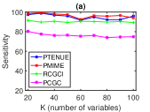
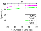
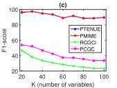
Figure 2: Accuracy indexes for S3 as a function of the number of variables $K$ as a mean over all time series lengths.

PMIME has the highest sensitivity, which stays at high levels for all $K$. PTENUE closely follows achieving also a high sensitivity for all $K$. The specificity of PTENUE is slightly highest than that of PMIME. A high specificity is achieved for the nonlinear measures that seems to be unaffected by the increase of the dimensionality. Overall, a high mean F1-score for all $K$ reflects the effectiveness of the two nonlinear measures. Indicatively, the extracted causal effects for S3 in $K=20$ variables with $n=2048$ based on the four measures is shown in Fig. 3, whereas also the percentage of detection of each causal link over all the realizations of the system is displayed.

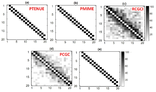
Figure 3: The heat matrix (gray scale) of the causality measure for all variable pairs of system S3 in $K=20$ variables with $n=2048$: (a) PTENUE, (b) PMIME, (c) RCGCI, (d) PCGC, (e) the true causal network.

The linear measures have a much inferior performance compared to the nonlinear ones. The influence of the time series length is more pronounced for the linear measures; their sensitivity increases with the time series length while specificity is reduced (see Table 10). RCGCI and PCGC (we increase $K_{S}$ from 4 ($K=20$) to 18 ($K=100$)) indicate the true causal influences, however suggest various indirect links as well as the spurious links $X_{2}\rightarrow X_{1}$ and $X_{K-1}\rightarrow X_{K}$. Their sensitivity is at a lower level than that of the nonlinear measures since they detect the causal links at a lower percentage over all the realizations. PCGC obtains the lowest sensitivity. Their specificity is also poorer compared to PMIME’s and PTENUE’s, but slightly increases with $K$ due to the decreasing percentages of indirect causal effects (see Fig. 2). Overall, a very low mean F1-score is reached by the linear measures which decreases with $K$.

3.2.5 Chaotic system with observational noise

The effect of noise on the four causality measures is examined by adding observational noise to the simulation system S3. In particular, we consider S3 in $K=5$ variables, fix the coupling strength to $c=0.2$ and change the noise levels to $10\%,20\%$ and $50\%$ (the noise standard deviation is a percentage of the noise-free data standard deviation). Moreover, different types of noise are considered: Gaussian white noise, white noise from t-Student distribution with 2 degrees of freedom (heavy tailed distribution) and noise given by a GARCH(1,1) system exhibiting volatility clusterings. The latter is defined as

$$e_{t} = \sigma_{t}w_{t}$$

$$\sigma_{t}^{2} = 0.2+0.2e_{t-1}^{2}+0.75\sigma_{t-1}^{2}$$

where $w_{t}$ is a Gaussian white noise process.

Figure 4 shows the results of the effect of the three noise types on the four causality measures for increasing noise levels (we set $n=2048$).

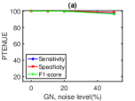
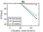
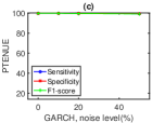
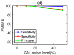
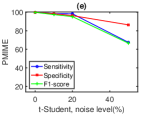
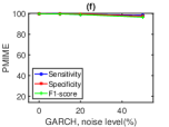
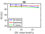
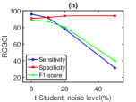
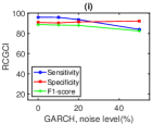
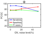
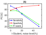
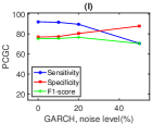
Figure 4: Accuracy indexes for S3 in $K=5$ variables and $c=0.2$, with increasing amplitude levels of observational noise for the three types of noise: Gaussian white noise (left column), t-Student (middle column) and GARCH(1,1) (right column), and for the four causality measures: PTENUE (first row), PMIME (second row), RCGCI (third row) and PCGC (fourth row).

The nonlinear measures are more stable to the effect of noise than the linear measures. For small noise levels, the performance of the measures is rather stable, but as the noise level rises, sensitivity decreases and therefore their overall performance gets worse. On the other hand, specificity slightly increases as the noise level grows showing the tendency of the measures to detect less links with the increase of noise level. The addition of noise from t-Student distribution seems to significantly affect all the measures, especially when noise level is high, where the PMIME is the least affected. Interestingly, the GARCH noise seems to affect only the linear measures, which shows high robustness to volatility clustering of the nonlinear measures.

4 Conclusions

In this study, a comparative analysis has been performed in order to evaluate an ensemble of well known causality measures. The robustness of the different measures is investigated on artificial data from multivariate systems with different characteristics. The main contribution of this study is the evaluation of an ensemble of different causality measures that have not been previously compared on simulation systems with different characteristics. Further, the study focuses on truly high dimensional systems of up to 100 variables. Finally, the noise robustness is examined, which is an essential part of this work since many comparative studies do not include noisy samples.

The evaluation of the causality measures showed differences in their performance in the different systems. First of all, the empirical results confirmed some generally recognized facts: a) the linear causality measures cannot systematically infer about the nonlinear causal effects and therefore their overall performance is worse than that of the nonlinear ones, b) bivariate causality measures indicate both direct and indirect causal effects while false indications of directed relationships often arise, c) fully conditioned causality measures are the most affected ones by the curse of dimensionality.

The main new findings of this study can be summarized to the following points:

• Partially conditioned measures (applying dimension reduction) are superior to bivariate and fully conditioned causality measures in both low and high dimensional systems. The utilization of the dimension reduction techniques to address the curse of the dimensionality seems indispensable when direct causality in multivariate time series is to be estimated.

• In total, PTENUE and PMIME are the optimal causality measures with similar performance at most cases. They seem to be robust, unaffected by the curse of dimensionality, the nature and the strength of the connections and the type of noise. Sufficiently long time series are though required to achieve their optimal performance. PTENUE is more robust in case of the stochastic systems; PMIME estimates slightly higher percentages than the nominal level ($5\%$) for the uncoupled pairs of variables and therefore its specificity is lower compared to PTENUE’s.

• The nonlinear measures are more stable to the effect of noise than the linear measures. In particular, the GARCH noise seems to affect only the linear measures. PMIME seems to be more robust to high levels of noise, especially of heavy tailed distribution.

It remains to be studied whether the optimal causality measures perform well also in systems with denser causality structures. Further, as a future work we aim to examine the performance of PTENUE and PMIME in comparison to different causal discovery methods, such as the Fast Causal Inference algorithm [62]. The effect of latent variables and instantaneous causality on the performance of the causality measures are also factors to be examined in future work.

References

- [1] K.J. Friston. Functional and effective connectivity: a review. Brain Connectivity, 1(1):13–36, 2011.
- [2] A.K. Seth, A.B. Barrett, and L. Barnett. Granger causality analysis in neuroscience and neuroimaging. Journal of Neuroscience, 35(8):3293–3297, 2015.
- [3] A. Papana, C. Kyrtsou, D. Kugiumtzis, and C. Diks. Financial networks based on Granger causality: a case study. Physica A - Statistical Mechanics and Its Applications, 482:65–73, 2017.
- [4] S.K. Stavroglou, A.A. Pantelous, K. Soramaki, and K. Zuev. Causality networks of financial assets. Journal of Network Theory in Finance, 3(2):17–67, 2017.
- [5] J.-C. Zheng and H.-K. Jiang. Correlation analysis and causality test between Ludong-Huanghai block and South Japan. Acta Seismologica Sinica, 20(4):381–391, 2007.
- [6] D. Chorozoglou, D. Kugiumtzis, and E. Papadimitriou. Testing the structure of earthquake networks from multivariate time series of successive main shocks in Greece. Physica A: Statistical Mechanics and its Applications, 499:28–39, 2018.
- [7] C.W.J. Granger. Investigating causal relations by econometric models and cross-spectral methods. Econometrica: Journal of the Econometric Society, pages 424–438, 1969.
- [8] C. Hiemstra and J.D. Jones. Testing for linear and nonlinear Granger causality in the stock price-volume relation. The Journal of Finance, 49(5):1639–1664, 1994.
- [9] T. Schreiber. Measuring information transfer. Physical Review Letters, 85(2):461, 2000.
- [10] C. Diks and V. Panchenko. A new statistic and practical guidelines for nonparametric Granger causality testing. Journal of Economic Dynamics and Control, 30(9-10):1647–1669, 2006.
- [11] D. Marinazzo, M. Pellicoro, and S. Stramaglia. Kernel method for nonlinear Granger causality. Physical review letters, 100(14):144103, 2008.
- [12] L. Barnett and A.K. Seth. The MVGC multivariate Granger causality toolbox: a new approach to Granger-causal inference. Journal of Neuroscience Methods, 223:50–68, 2014.
- [13] A. Papana, C. Kyrtsou, D. Kugiumtzis, and C. Diks. Detecting causality in non-stationary time series using partial symbolic transfer entropy: evidence in financial data. Computational Economics, 47(3):341–365, 2016.
- [14] L.A. Baccalá and K. Sameshima. Partial directed coherence: a new concept in neural structure determination. Biological Cybernetics, 84(6):463–474, 2001.
- [15] A. Korzeniewska, M. Manczak, M.and Kaminski, K. Blinowska, and S. Kasicki. Determination of information flow direction between brain structures by a modified directed transfer function method (dDTF). Journal of Neuroscience Methods, 125:195–207, 2003.
- [16] G. Nolte, A. Ziehe, V.V. Nikulin, A. Schlögl, N. Krämer, T. Brismar, and K.-R. Müller. Robustly estimating the flow direction of information in complex physical systems. Physical Review Letters, 100(23):234101, 2008.
- [17] G. Nolte, A. Ziehe, N. Krämer, F. Popescu, and K.-R. Müller. Comparison of Granger causality and phase slope index. In NIPS Causality: Objectives and Assessment, 2010.
- [18] M. Vinck, R. Oostenveld, M. Van Wingerden, F. Battaglia, and C.M.A. Pennartz. An improved index of phase-synchronization for electrophysiological data in the presence of volume-conduction, noise and sample-size bias. Neuroimage, 55(4):1548–1565, 2011.
- [19] K.J. Blinowska, R. Kuś, and M. Kamiński. Granger causality and information flow in multivariate processes. Physical Review E, 70(5):050902, 2004.
- [20] J. Geweke. Measurement of linear dependence and feedback between multiple time series. Journal of the American Statistical Association, 77(378):304–313, 1982.
- [21] L. Angelini, M. De Tommaso, D. Marinazzo, L. Nitti, M. Pellicoro, and S. Stramaglia. Redundant variables and Granger causality. Physical Review E, 81(3):037201, 2010.
- [22] D. Marinazzo, M. Pellicoro, and S. Stramaglia. Causal information approach to partial conditioning in multivariate data sets. Computational and Mathematical Methods in Medicine, 2012(303601), 2012.
- [23] L. Breiman. Better subset regression using the nonnegative garrote. Technometrics, 37(4):373–384, 1995.
- [24] D. Collins and S. Gavron. Channels of financial market contagion. Applied Economics, 36(21):2461–2469, 2004.
- [25] Y. Yang and L. Wu. Nonnegative adaptive lasso for ultra-high dimensional regression models and a two-stage method applied in financial modeling. Journal of Statistical Planning and Inference, 174:52–67, 2016.
- [26] I. Brüggemann. Measuring monetary policy in Germany: a structural vector error correction approach. German Economic Review, 4(3):307–339, 2003.
- [27] A. Shojaie and G. Michailidis. Discovering graphical Granger causality using the truncating lasso penalty. Bioinformatics, 26(18):i517–i523, 2010.
- [28] E. Siggiridou and D. Kugiumtzis. Granger causality in multivariate time series using a time-ordered restricted vector autoregressive model. IEEE Transactions on Signal Processing, 64(7):1759–1773, 2015.
- [29] I. Vlachos and D. Kugiumtzis. Nonuniform state-space reconstruction and coupling detection. Physical Review E, 82(1):016207, 2010.
- [30] L. Faes, G. Nollo, and A. Porta. Information-based detection of nonlinear Granger causality in multivariate processes via a nonuniform embedding technique. Physical Review E, 83(5):051112, 2011.
- [31] D. Kugiumtzis. Direct-coupling information measure from nonuniform embedding. Physical Review E, 87(6):062918, 2013.
- [32] M. Songhorzadeh, K. Ansari-Asl, and A. Mahmoudi. Two step transfer entropy - an estimator of delayed directional couplings between multivariate EEG time series. Computers in Biology and Medicine, 79:110–122, 2016.
- [33] Maciej Kamiński, Mingzhou Ding, Wilson A Truccolo, and Steven L Bressler. Evaluating causal relations in neural systems: Granger causality, directed transfer function and statistical assessment of significance. Biological Cybernetics, 85(2):145–157, 2001.
- [34] E. Siggiridou, C. Koutlis, A. Tsimpiris, and D. Kugiumtzis. Evaluation of Granger causality measures for constructing networks from multivariate time series. Entropy, 21(11):1080, 2019.
- [35] M.-H. Wu, R.E. Frye, and G. Zouridakis. A comparison of multivariate causality based measures of effective connectivity. Computers in Biology and Medicine, 41(12):1132–1141, 2011.
- [36] E. Florin, J. Gross, J. Pfeifer, G.R. Fink, and L. Timmermann. Reliability of multivariate causality measures for neural data. Journal of Neuroscience Methods, 198(2):344–358, 2011.
- [37] A. Fasoula, Y. Attal, and D. Schwartz. Comparative performance evaluation of data-driven causality measures applied to brain networks. Journal of Neuroscience Methods, 215(2):170–189, 2013.
- [38] A. Papana, C. Kyrtsou, D. Kugiumtzis, and C. Diks. Simulation study of direct causality measures in multivariate time series. Entropy, 15(7):2635–2661, 2013.
- [39] K.J. Blinowska. Review of the methods of determination of directed connectivity from multichannel data. Medical & Biological Engineering & Computing, 49(5):521–529, 2011.
- [40] M.J. Silfverhuth, H. Hintsala, J. Kortelainen, and T. Seppänen. Experimental comparison of connectivity measures with simulated EEG signals. Medical & Biological engineering & Computing, 50(7):683–688, 2012.
- [41] E. Olejarczyk, L. Marzetti, V. Pizzella, and F. Zappasodi. Comparison of connectivity analyses for resting state EEG data. Journal of Neural Engineering, 14(3):036017, 2017.
- [42] S. Guo, A.K. Seth, K.M. Kendrick, C. Zhou, and J. Feng. Partial Granger causality - eliminating exogenous inputs and latent variables. Journal of Neuroscience Methods, 172(1):79–93, 2008.
- [43] V.A. Vakorin, O.A. Krakovska, and A.R. McIntosh. Confounding effects of indirect connections on causality estimation. Journal of neuroscience methods, 184(1):152–160, 2009.
- [44] J. Runge. Conditional independence testing based on a nearest-neighbor estimator of conditional mutual information. In International Conference on Artificial Intelligence and Statistics, pages 938–947, 2018.
- [45] J. Zhang. Low-dimensional approximation searching strategy for transfer entropy from non-uniform embedding. PloS one, 13(3), 2018.
- [46] Z. Jia, Y. Lin, Z. Jiao, Y. Ma, and J. Wang. Detecting causality in multivariate time series via non-uniform embedding. Entropy, 21(12):1233, 2019.
- [47] T. Li, G. Li, T. Xue, and J. Zhang. Analyzing brain connectivity in the mutual regulation of emotion - movement using bidirectional Granger causality. Frontiers in Neuroscience, 14, 2020.
- [48] A. Papana, D. Kugiumtzis, and P.G. Larsson. Detection of direct causal effects and application to epileptic electroencephalogram analysis. International Journal of Bifurcation and Chaos, 22(09):1250222, 2012.
- [49] D. Kugiumtzis. Partial transfer entropy on rank vectors. The European Physical Journal Special Topics, 222(2):401–420, 2013.
- [50] A. Montalto, L. Faes, and D. Marinazzo. MuTE: a MATLAB toolbox to compare established and novel estimators of the multivariate transfer entropy. PloS one, 9(10), 2014.
- [51] J. Kořenek and J. Hlinka. Causal network discovery by iterative conditioning: comparison of algorithms. Chaos: An Interdisciplinary Journal of Nonlinear Science, 30(1):013117, 2020.
- [52] N. Wiener. The theory of prediction. Modern Mathematics for Engineers, 58:323–329, 1956.
- [53] L. Barnett, A.B. Barrett, and A.K. Seth. Granger causality and transfer entropy are equivalent for Gaussian variables. Physical Review Letters, 103(23):238701, 2009.
- [54] K. Hlavácková-Schindler. Equivalence of Granger causality and transfer entropy: a generalization. Applied Mathematical Sciences, 5(73):3637–3648, 2011.
- [55] A. Kraskov, H. Stögbauer, and P. Grassberger. Estimating mutual information. Physical Review E, 69(6):066138, 2004.
- [56] A.K. Seth. A MATLAB toolbox for Granger causal connectivity analysis. Journal of Neuroscience Methods, 186(2):262–273, 2010.
- [57] R. Quian Quiroga, A. Kraskov, T. Kreuz, and P. Grassberger. Performance of different synchronization measures in real data: a case study on electroencephalographic signals. Physical Review E, 65(4):041903, 2002.
- [58] G.-H. Yu and C.-C. Huang. A distribution free plotting position. Stochastic Environmental Research and Risk Assessment, 15(6):462–476, 2001.
- [59] B. Schelter, M. Winterhalder, M. Eichler, M. Peifer, B. Hellwig, B. Guschlbauer, C.H. Lücking, R. Dahlhaus, and J. Timmer. Testing for directed influences among neural signals using partial directed coherence. Journal of Neuroscience Methods, 152(1-2):210–219, 2006.
- [60] A. Politi and A. Torcini. Periodic orbits in coupled hénon maps: Lyapunov and multifractal analysis. Chaos: An Interdisciplinary Journal of Nonlinear Science, 2(3):293–300, 1992.
- [61] C. Koutlis, V.K. Kimiskidis, and D. Kugiumtzis. Identification of hidden sources by estimating instantaneous causality in high-dimensional biomedical time series. International Journal of Neural Systems, 29(04):1850051, 2019.
- [62] D. Entner and P.O. Hoyer. On causal discovery from time series data using FCI. Probabilistic Graphical Models, pages 121–128, 2010.