Essential Scattering Applications for Everyone. Overview.

Abstract

ESCAPE is a free python package and framework for creating applications for simulating and fitting of X-ray and neutron scattering data with current support for specular reflectivity, polarized neutron reflectometry, high resolution X-ray diffraction, small angle scattering with future support for off-specular scattering from structured samples with complicated morphology. Utilizing current features of Jupyter project (https://jupyter.org/), it allows to create highly customized applications in the format of notebooks. These notebooks, being shared with other users, can be used directly or started as web applications with graphical user interface. This paper is a brief overview of the core and scattering packages providing description of the major features with code examples. The following features make ESCAPE different from other projects: independent from scattering applications core, which provides access to models building blocks like parameters, variables, functors, data objects, models and optimizers; support of arithmetic operations and algebraic expressions on parameters and functors, offering models with complex dependencies of parameters; math module with standard mathematical functors and special functors which perform numerical integration over variable or parameter, supplying customization of intensity model; simultaneous fit of several models, also for models with different dimensions. Check our web site https://escape-app.net/ for further information.

1 Introduction

Due to continuously increasing number of industrial and scientific utilization of scattering methods in condensed-matter (Orji et al., 2018) and soft-matter (Müller-Buschbaum, 2013) branches it is important to provide for potential users a flexible, highly customizable and relatively fast software for data analysis.

Scattering problems like small angle scattering, or grazing incidence small angle scattering, specular reflectivity, diffraction, X-ray fluorescence etc., differ significantly not only in terms of theory and experiment handling, but also in data preparation and visualization.

Many existing applications are dedicated for a particular sample type and particular scattering method. As a result users have to deal with several data formats, several optimization routines, several, sometimes not obvious, workflows.

Application of new data analytics such as big data handling, deep learning, artificial intelligence techniques require easy integration of modelling and simulation routines to the existing frameworks and infrastructure (see report IEEE (2018)).

Developing a software which successfully resolves all issues and satisfies advanced users and beginners is a challenging task.

In this publication we give an overview for the Essential Scattering Applications for Everyone (ESCAPE), a private independent project. ESCAPE is compiled as a python package which, compared to other existing scattering applications (Lazzari (2002), Bressler et al. (2015), Pospelov et al. (2020)) provides a set of common interfaces with the same look and feel for different scattering techniques fully integrated by default with the Jupyter notebook environment.

The development of this software and its first early prototype dates back to 2012. The idea of the software concept came in author’s mind during High Data Rate Initiative sessions (https://www.pni-hdri.de). ESCAPE is dedicated first of all to experienced physicists - scattering instrument or laboratory responsibles, people who understand in details scattering techniques, data preparation and required scattering formalism for obtaining successful results. With ESCAPE they can prepare a set of customized applications (also with graphical user interface) for different experimental setups and share these applications with less experienced users. After publication of results users can share their experience with others simply publishing notebooks in our repository, check our webpage https://escape-app.net for more details. As a result everyone can use shared notebooks for educational purposes, training and planning of future experiments, simulating experimental curves for new samples and playing with settings and parameters of models. The present paper focuses on a general concept of ESCAPE and core features.

2 Overview

2.1 License and collaborative work

ESCAPE is released closed source and is free for non-commercial usage. Free availability together with widely used Jupyter notebook (Kluyver et al, 2016) file format provides full verifiability of obtained results. A clear, continuously developed python modules allows experienced users to adapt ESCAPE to their own needs.

Examples of notebooks are published under GNU General Public License version 3. Users of ESCAPE project are encouraged to share their notebooks with published scientific results. The published notebooks give information about most often usage cases of ESCAPE, inducing authors for further improvement of available modules and resolving issues.

2.2 Programming languages

Different programming languages have been created for different purposes and in ESCAPE we try to use programming languages in the most effective way. The core of ESCAPE is a template, header only library written in C++, using standard C++17. C++ language provides good performance and parallel computation. The core is fully independent of any other libraries providing relatively small compiled size of the package. Python bindings are developed with Cython. For most of the C++ classes in the core there is a wrapper Cython class. This wrapper classes are visible for users and define the package functionality available for users. Cython wrappers are split into several modules and compiled for Linux, MacOS and Windows platforms as Python whl installation archives. ESCAPE has also escape.utils package with useful specific modules and routines to simplify some usage cases. This includes material database, based on periodictable package and special commands for calling compact, integrated with notebooks widgets to simplify certain routines.

As a result, for users who are familiar with Python itself and scientific Python packages like scipy (Virtanen et al., 2020), numpy (van der Walt et al., 2011), matplotlib (Hunter, 2007), etc., the learning curve will be shallow. For others, it will be another good reason to learn one of the most popular platforms nowadays.

2.3 Core package overview

In order to describe a core functionality and the main philosophy of ESCAPE package, we provide in this section a simple example. Imagine that you have some experimental Small Angle Scattering Data from silica particles of spherical shape. You would like to create a model and to fit these data. Creation of a model in ESCAPE starts with definition of parameters. A standard scattering form-factor of a spherical particle is given by the following equation

$$F(q)=3\frac{\sin(qR)-qR\cos(qR)}{(qR)^{3}}$$ (1)

where $q$ is a length of scattering vector, $R$ is a particle radius.

The measured intensity is given as following

$$I(q)=N\Delta\eta^{2}V^{2}|F|^{2}+B$$ (2)

where $N$ is the number density of particles, $V=4/3\pi R^{3}$ is the volume of the particles, $\Delta\eta$ - scattering length density contrast and $B$ - constant background.

We define parameters of the model, variable and intensity functor, i.e. function object, as following

⬇

import numpy as np

from escape.utils import show

R = esc.par("R", 7.5, units="nm")

C = esc.par("Contrast", 1.2, scale=1e-3,

units="nm^-2")

B = esc.par("Background", 4, units="arbitr")

N = 1e5

q = esc.var("q")

V = 4/3*np.pi*esc.pow(R, 3)

F = 3*(esc.sin(q*R)-q*R*esc.cos(q*R))/

(esc.pow(q*R, 3))

I = N*esc.pow(C*V*F, 2.0)+B

show(I, coordinates=np.arange(0, 4.0, 0.001),

ylog=True,

ylabel=’I’, xlabel=’Q[1/nm]’,

title="Intensity: Spherical particle")

A result of this code is a widget (see Figure 1), with controls to change parameters values on the right side and resulting plot of intensity.

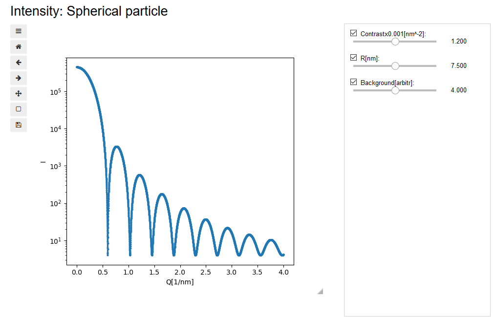
Figure 1: Widget for the intensity functor.

Next we open the experimental data using numpy.loadtxt routine and create data object dobj- container for experimental data. Model object mdl calculates simulated model curves and can compare them with experimental data by means of the cost function. For the optimization we are going to use Levenberg-Marquardt optimizer (see section 2.3.6).

⬇

unpack=True)

dobj = esc.data("Data", x, y, copy=True)

mdl = esc.model("Model", I, dobj)

opt = esc.levmar("LM", mdl)

show(opt, ylog=True,

ylabel=’I’, xlabel=’Q[1/nm]’,

title="Intensity fitting")

Resulted widget (see Figure 2) provides the plot with a cost function history and can be used to start/interrupt optimization process and save/load parameters values with estimated errors.

Figure 2: Widget for the optimizer

As it has been already mentioned, a user should not create such a notebook from scratch. For the beginning we have plenty of example notebooks for all kind of available applications.

2.3.1 Parameters

Internally ESCAPE package operates with several parameter handlers of two sorts: independent parameters, which are recognized for optimization and dependent parameters, which have, for example, a form of arithmetic expression and depend on parameters of the first type.

Practically both groups of parameters are hidden behind the same object type and user can use a dependent parameter of any complexity where appropriate. This gives a lot of freedom for definition of complex problems where independent parameters being a part of complex expression are shared between different objects, like layers in multilayer samples, for example, or even between different models, which can be fit simultaneously.

2.3.2 Functors

Functors are objects which behave like functions, i.e. they have a call operator. In ESCAPE we tried to make functors definition as simple as writing a formula. Functors support up to five variables, which is enough for scattering applications implemented in ESCAPE. On request, the number of variables can be easily increased.

Functors in ESCAPE can be defined as a mathematical expression, like spherical form-factor we presented above. More complicated functors, for calculation of intensities or averaging, etc. are implemented in C++ core and created by user using special factory functions. Functors support arithmetic operations which provides a flexible way of customizing intensity calculation with specific diffuse scattering, background with scattering vector dependency, illumination correction, resolution effects, etc.

Most of the functors in ESCAPE return float values when being called, but additionally, there is a support for complex functors which operates real type variables but return complex values.

2.3.3 Math

Parameters and functors in ESCAPE support arithmetic operations and mathematical functions. Additionally to standard mathematical functions like $\exp$, $\log$, $\mathrm{pow}$, $\sin$, $\cos$, etc., there are also special functors implemented which perform numerical integration over variable of an integrated functor or its parameter. This gives a possibility for integrating of intensity over resolution function, or averaging integration over certain parameter and its distribution. In the examples available online, we provide notebooks which demonstrate usage of such integral functors, over parameter and variable, for example, for the intensity simulation from bimodal silica nanoparticles with size distribution, like in the paper Breßler et al.(2015). Integral functors support two integration methods: with fixed number of quadrature points and adaptive. The characteristic width of distribution function in the case of averaging integration can be defined as a functor of integration variable, which allows to perform integration for the cases of instrumental resolution function with varying full width of a half maximum.

2.3.4 Data

Data object is a container which prepares experimental data for optimization. Currently there is only generic implementation which can handle provided arrays of coordinates, intensities and errors. Automatic reading of experimental data from a file is specific for every instrumental setup and is not supported currently. If experimental file has a format of a text tabulated data, users can try to open it using numpy python library. Errors of intensities can be provided as an array or will be calculated from intensity values according to Poisson statistics as $\sqrt{I}$ by default. The correctness of provided data errors defines the correctness of estimated parameters errors, made after fitting. Data object also supports masking of experimental data, which allows to ignore points with detector failures, cosmic rays, primary beam and other parasitic features.

2.3.5 Model

The main task of the model object is to make a quantitative comparison of results returned by the functor, i.e. simulation curve, with experimental data returned by the data object. This comparison is made by means of residuals and well-known $\chi^{2}$ cost function which is given by

$$\chi^{2}=\frac{1}{N-M}\sum_{i=1}^{N}\left[\frac{I_{\mathrm{exp}(q_{i})}-I_{\mathrm{mod}(q_{i})}}{\sigma_{\mathrm{exp}(q_{i})}}\right]^{2}$$ (3)

The intensities in equation 3 can be scaled, which is important if there is a power low of intensity values or there is a strong peak in experimental data which is several magnitudes stronger than intensity values in its neighbourhood. Model object provides several scaling options for residuals: logarithmic scale of intensity, and scaling of intensity with the scattering vector of power two or four. In future we plan to add a support for fully custom, user defined scaling functors. The residuals scaling is used for the calculation of cost function during the fit, estimation of errors is done always with standard cost function without scaling.

2.3.6 Optimizer

Among most of existing optimizers we have chosen Levenberg-Marquardt - well-known damped least-squares optimization method suitable for most of the scattering problems and Differential Evolution (DE) method, stochastic method, which is very simple to implement and to extend.

The Levenberg-Marquardt optimization algorithm (Levenberg, 1944; Marquardt, 1963) is a least-squares method which interpolates between Gauss-Newton method and gradient- descent and is known to converge fast to the local minimum of the cost function.

Scattering problems, especially for multilayer, could have a large number of parameters, and depending on quality of experimental data it could lead to several cost function minima in the search domain. If constrains of parameters are too wide and initial model curve is too far away from experimental curve, this can lead to instabilities in found solution.

To prevent possible instabilities it is required to start iterative LMA optimization when the model intensity is close to experimental values. This is quite often considered as the main disadvantage of LMA optimization method.

In contrast differential evolution method is a meta-heuristic method, it doesn’t require optimization problem being differentiable and depending on settings can search larger spaces of candidate solutions comparing to LMA.

The method of differential evolution was developed by Price and Storn (see Storn et al., 1997). To our knowledge, the first usage of this algorithm for scattering applications is described in Ref. Wormington et al. (1999). The idea of this algorithm is the following: initially a population of points $p$ in $m$-dimensional space is generated and cost function is evaluated for each point. Then at each iteration for each point $p_{i}$ three different points $p_{a}$, $p_{b}$ and $p_{c}$ are randomly chosen from the population. The next step is a mutation - a new point $p_{n}$ is constructed from these three points as following $p_{n}=F(p_{b}-p_{c})+p_{a}$ with a probability of crossover setting $Cr$. If a cost function for a new point $p_{n}$ has a better value than the currently chosen $p_{i}$, than it replaces $p_{i}$. If not than $p_{i}$ remains. Thus on each iteration we obtain a population with points which are better or as good as previous. The process is repeated until maximum number of iterations is reached.

We have slightly extended our implementation of DE optimizer. There are two polishing scenarios for parameters: final polishing after DE optimization and candidate polishing, when point candidate is succesfully chosen to replace $p_{i}$ in population set. Both are done with LMA optimizer and for both one can set maximum iteration number. In the latter case polishing with only few iterations could improve convergence and reduce number of function evaluations in our tests. This also resolves partly the main disadvantage of DE compared to LMA - a slower convergence and quite high number of function evaluations. DE in most cases is not sensitive to initial solution and is not easily trapped by local minimum like LMA. But still there is no guarantee that DE will find global minimum.

2.3.7 Machine learning. Regressor

A solution for typical inverse problems like scattering applications, can be found not only by means of optimization, i.e. comparison between measured and simulated intensity. Encouraged by work of Glorieux et al. (2001), we present here a regressor to solve inverse problems by means of neural network regression algorithms. The corresponding class plays a role of an interface for any regressor written in python, which satisfies certain functionality. As a basis for this interface we took MLPRegressor class from sklearn.neural_network package. Below is an example of how to use regressor with an existing model.

⬇

rgi = MLPRegressor(max_iter=1000,

solver="adam",

activation="relu")

def noisify(X):

X = np.asarray(X)

X = np.random.poisson(X)

return X

def normalize(X):

X = np.asarray(X)

X = np.log10(X*N+1)

X = X/np.max(X)

return X

rg = esc.regressor("Regressor",

mobj, 1500, 150,

impl=rgi,

norm_method=normalize,

noisify_method=noisify)

show(rg, ylog=True)

We create first the MLPRegressor object from sklearn.neural_network with adam solver, which refers to stochastic gradient-based optimizer, and relu activation function for the hidden layer, which returns $f(x)=max(0,\;x)$. A complete list of all arguments and their possible values can be found in the official documentation for the sklearn.neural_network package. Next we define two methods, noisify and normalize which modify the generated data by adding Poisson noise, scale and normalize the intensity values. Particularly, the noisify method adds the Poisson noise to the data and normalize method performs logarithmic scaling and normalization to the maximum value. The created MLPRegressor instance together with the data modification methods are the input parameters of escape.regressor factory function. Before regressor will be able to make any prediction it must be trained first. The request for the training can be done in the widget (see Figure 3) by pressing corresponding button or by calling a corresponding train function of the created instance. Before training regressor wrapper generates a certain number of experimental data sets, $1500$ in our case, by changing model parameters randomly and applies noisify and normalize methods to the data arrays, then it starts the training procedure of the MLPRegressor instance on the generated and modified dataset. Together with the training data set regressor generates the test data set to calculate the training error. The regressor widget allows user to check prediction results for the test data set. After training user can perform prediction of parameters for real experimental data by calling regressor object as rg(dobj), where dobj is a data object, containing experimental data arrays. The data normalization method provided during creation of regressor instance will also be applied to the experimental data.

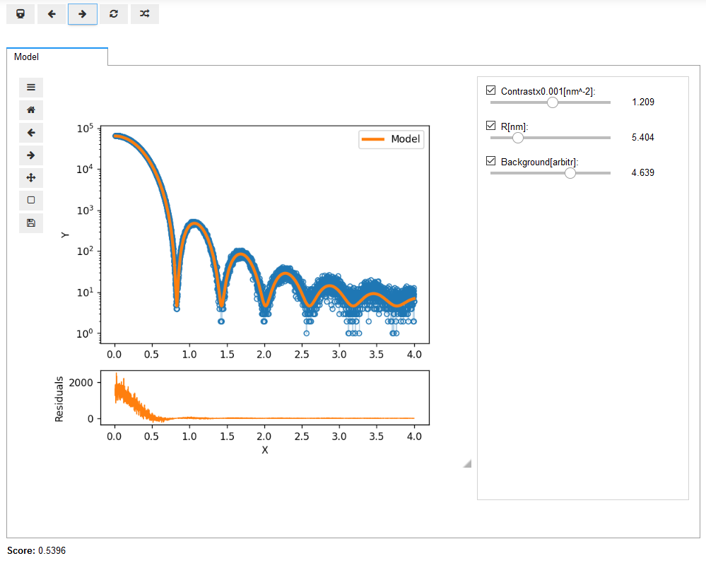
Figure 3: Widget for the neural networks regressor object.

Prediction quality is not perfect and depends on the number of training datasets and number of free parameters in the model. Overall, our conclusions are not far away from the conclusions presented in Glorieux et al.(2001), where neural networks regressor was applied to HRXRD model with gradient layer. The number of sublayers used to describe a gradient of SLD was also one of the justified parameters during regression. ESCAPE currently doesn’t allow that and predicts only parameters of the model, i.e. quantitative model characteristic. But, certainly, the implementation of prediction of qualitative model settings, such as number of layers, gradient function, roughness model, etc., is of our great interest.

The regressor doesn’t guarantee perfect result, but can be used for preliminary estimation of model parameters before fitting. It can reduce number of optimizer iterations needed for convergence of optimizer to the minimum of the cost function and can be effectively used for the batch processing, i.e. for the large number of experimental data obtained from the same type of sample, which is a typical industrial application.

2.4 Scattering package overview

The scattering package contains components for material and sample description as well as functors for calculation of intensity for different scattering applications. Currently sample description objects are dedicated for layered samples with homogeneous layers and layers with gradients of material parameters, like scattering length density, strain, etc. The support for structured samples comes together with potential module, which is experimental currently.

As we have already mentioned, all scattering problems in ESCAPE are implemented in terms of functors. The variables for this functors are provided by user and for scattering applications these variables are always reciprocal space coordinates, like components of scattering vector or scattering vector length.

ESCAPE doesn’t operate entities like scans types or description of experimental setup, like detectors or slits.

These entities are very specific to experimental setups and in most cases users can easily convert real-space parameters of performed experiment, like forthcoming and outgoing angles of the primary and scattered beam to corresponding reciprocal space coordinates of scattering events on the detector. Below we give a brief overview of scattering package modules.

2.4.1 Materials

The speed of propagation of plane waves in the medium is slower than in vacuum. The index of refraction is a commonly used characteristic of material, which is equal to ratio between the speed of wave in vacuum and inside a medium. For a homogeneous material it is defined as following

$$n=1-\delta+i\beta$$ (4)

Parameters $\delta$ and $\beta$ are very well-known in optics and usually are used to characterize a material in scientific software packages for X-ray scattering. Both parameters depend on composition of medium and wavelength of incident wave.

In ESCAPE we use Scattering Length Density (SLD), both real and imaginary (absorption) parts, as default fit parameters. SLD is more popular in neutron scattering community and conversion between terms of refractive index and SLD is the following:

$$\delta=\frac{\lambda^{2}}{2\pi}\mathrm{Re}(SLD);\quad\beta=\frac{\lambda^{2}}{2\pi}\mathrm{Im}(SLD)$$ (5)

Another approach, very popular in commercial applications is to fit a mass density instead of refractive index terms. This approach is also available in ESCAPE using the material database package (see escape.utils.mdb). A composition of material can be provided as a chemical formula, in the same way as in periodictable package, which is used by the module. The resulted material instance depends on mass density parameter provided by user. Both SLDs, real and imaginary part are calculated from the mass density. It reduces the number of fit parameters, but from our experience work good only for the cases of perfect quality samples, when composition of an investigated sample is known.

ESCAPE allows to work with both approaches and to apply them simultaneously for creation of material objects.

Below we define two material objects for Fe and Si ignoring for simplicity their absorption scattering length density parameters

⬇

scale=1e-4, units="1/nm^2")

Si_sld=esc.par("Si SLD", 2.074,

scale=1e-4, units="1/nm^2")

Fe = esc.amorphous("Fe", Fe_sld, 0.0)

Si = esc.amorphous("Si", Si_sld, 0.0)

2.4.2 Layered sample

The modelling of intensity cannot be done without sample description. For this purposes ESCAPE operates several objects of the following types: layer, layerstack and multilayer. The layer instance is used for description of a single layer and requires material, thickness parameter and root mean square roughness parameter. In the code listing below we create three layer objects forming trilayer Fe/Si/Fe with zero roughness. The Fe layers share the same material object and, thus, there SLDs parameters are also shared.

⬇

thknFe2 = esc.par("Fe Thkn 2", 10, units="nm")

thknSi = esc.par("Si Thkn", 1, units="nm")

#zero roughness

Fe_layer1 = esc.layer("Layer: Fe 1", Fe,

thknFe1, 0.0)

Fe_layer2 = esc.layer("Layer: Fe 2", Fe,

thknFe2, 0.0)

Si_layer = esc.substrate("Substrate: Si", Si, 0.0)

If multilayered sample consists of stack of several layers repeated many times, layerstack object should be used which takes number of repeats of the stack in the multilayer sample.

Stacks and layers should be added to multilayer object as following

⬇

Si_sub = esc.amorphous("Si", 2.074e-4, 0.0)

air = esc.air("Air")

sub = esc.substrate("Substrate: Si", Si_sub, 0.0)

sample = esc.multilayer("Fe/Si/Fe", air, sub)

sample.add(Fe_layer1)

sample.add(Si_layer)

sample.add(Fe_layer2)

show(sample, xlabel="Z[nm]",

ylabel="SLDRe[1/nm^2]", yaxis="sld0re")

The substrate material we left with constant standard value of SLD. Background (substrate) and foreground (air) layers both have zero roughness and no fit parameters. When being added new layers are always inserted between the substrate and the last layer. Indexing of layers starts from the first layer after foreground down to the substrate. The last command in the code listing will show the widget with a plot for real part of scattering length density profile.

2.4.3 Specular reflectivity

Specularly reflected intensity from a multilayer with rough interfaces can be calculated in terms of dynamical, semi-kinematic and kinematic approximations of scattering theory. A good review of these approximations with a full list of references and their application to specular and off-specular reflectivity can be found in the thesis of Petr Mikulik, 1997. For the dynamical theory there are two formalisms exist: transfer matrix formalism and Parratt formalism. The latter is the default formalism for the modelling of specular reflectivity in ESCAPE.

Semi-kinematic approximation takes into account only single reflection in every layer and, thus, gives wrong result near the angle of total reflection. The kinematic approximation doesn’t take into account absorption of incident and reflected wave inside the layers and fail for thick samples also at higher angles.

Functor object which calculates specular reflectivity using transfer matrix formalism is created as following

⬇

R = esc.specrefl("Specrefl", Qz,

sample,

formalism="matrix")

2.4.4 Polarized neutron reflectivity

Polarized-neutron specular reflectometry (PNR) allows to measure depth-resolved magnetization in flat films with characteristic thicknesses from 2 to 5000 Å. This method has been widely used to study homogeneous and heterogeneous magnetic films, as well as superconductors. The off-specular reflectivity scans allow to characterize lateral magnetic structures.

Implementation of Polarized Neutron Reflectivity functor is based on the following publications: Rühm et al. (1999), Kentzinger et al.(2008).

In ESCAPE, we provide a functor which accepts as input parameters efficiencies for polarization and analysis. The sign of this parameter defines a direction of polarization. Reflectivity functors which includes all four channels $++$, $--$, $+-$, $-+$ for simultaneous fit can be defined as following

⬇

#polarization efficiency

poleffi = esc.par("Poleff_i", 1)

polefff = esc.par("Poleff_f", 1)

#flipper efficiency

flipeffi = esc.par("Flipeff_i", 1)

flipefff = esc.par("Flipeff_f", 1)

Rpp = esc.pnrspec("R++", Qz, sample,

poleffi, polefff)

Rpm = esc.pnrspec("R+-", Qz, sample,

poleffi, -polefff*flipefff)

Rmp = esc.pnrspec("R-+", Qz, sample,

-poleffi*flipeffi, polefff)

Rmm = esc.pnrspec("R--", Qz, sample,

-poleffi*flipeffi,

-polefff*flipefff)

where sample is a layered sample object. This functors can be added to model objects and fit later simultaneously. This approach allows to avoid additional experimental data correction. If efficiency is known, values of corresponding parameters might be corrected manually and fixed or set as constant values to disable their optimization.

2.4.5 High resolution X-ray diffraction

Next functor which we would like to present is for simulating dynamical x-ray diffraction from strained crystals, multilayers, and superlattices. Its implementation is based on publication of Stepanov et al. (1998) and is based on two-beam approximation. This functor provides solution only for scans near a single diffraction peak. There are implementations for two approximations available: 4x4 matrix algorithm - valid for a full range of outgoing angles, including low angles, where reflection amplitudes are strong; 2x2 matrix algorithm - valid for high angles, where reflection amplitudes are negligible. The first one is normally used for modelling of diffraction at grazing incidence and the second one for the conventional diffraction scans.

The functor can simulate the following structural properties in multilayer: characteristic of material, like SLDs, normal lattice strains, interface roughness.

For the simulation of lateral strain effects additional scripting is necessary, an example notebook is in preparation. The current implementation cannot be used for scans far away from the Bragg peaks and for the scans which include several diffraction peaks. Currently there is no implementation of kinematic and semi-kinematic approximations. We plan to add them in future versions together with support for structured samples.

2.4.6 Structured samples. Potential

The potential module is a basis for description of structured samples. It is currently experimental and has been probed only for Small Angle Scattering applications, but certainly will be developed further and used for Diffraction, Grazing Incidence, and Off-specular Reflectivity from structured samples. The advantage of this module is a possibility to create complicated structures by means of arithmetic operations on potentials. After releasing, users will be able to build lithographically structured samples with a complexity comparable with samples presented in Sunday et al.(2019).

Imagine that we would like to get the potential object of a structure unit consisting of two rectangular fins, located at distance $D$ from each other. A regular lattice of such fins can be a part of semiconductor device used in electronics. So, it is not far away from real application. Each fin has a width of $w_{x}=25\,nm$, and consist of silicon core covered with $2.5\,nm$ hafnium oxide. We create first two materials objects as following

⬇

si = esc.amorphous("Si", 20.071e-6,

-0.458e-6)

hfo2 = esc.amorphous("HfO2", 63.976e-6,

-4.178e-6)

Next we create necessary parameters for silicon core and hafnium oxide shape.

⬇

wy_f = esc.par("wy f", 500, units="nm")

wz_f = esc.par("wz f", 100, units="nm")

wx_c = esc.par("wx c", 20, units="nm")

wy_c = esc.par("wy c", 500, units="nm")

wz_c = esc.par("wz c", 97.5, units="nm")

D= esc.par("D", 75, units="nm")

And now we are ready to create potential objects. Calculation of potential of structured samples is easy to define in terms of the shape function $\Omega(\mathbf{r})$. For the fin structure we are trying to describe the equation for the potential can be given as following

$$V(\mathbf{r})=V_{o}\Omega_{f}(\mathbf{r})-V_{o}\Omega_{c}(\mathbf{r})+V_{c}\Omega_{c}(\mathbf{r})$$ (6)

where $\Omega_{f}(\mathbf{r})$ is a shape function of the whole fin, $V_{o}$ - constant potential of Hafnium Oxide, $\Omega_{c}(\mathbf{r})$ - shape function of the core, $V_{c}$ - constant potential of the core. In the first part of equation we create a hollow rectangular fin by extracting from the whole Hafnium Oxide fin its core part and then adding the core shape again but with silicon potential $V_{c}$. In ESCAPE each term in equation 6 correspond to potential object as following

⬇

wx_f, wy_f, wz_f,

pos=[(-D/2, 0, wz_f/2),

(D/2, 0, wz_f/2)])

V_oc = esc.box("", qx, qy, qz, hfo2,

wx_c, wy_c, wz_c,

pos=[(-D/2, 0, wz_c/2),

(D/2, 0, wz_c/2)])

V_cc = esc.box("", qx, qy, qz, si,

wx_si, wy_c, wz_c,

pos=[(-D/2.0, 0, wz_c/2),

(D/2.0, 0, wz_c/2)])

V_hol = V_of - V_oc

V = V_hol + V_cc

show(V_hol, title="Hollow fin")

show(V, title="Filled fin")

where $V_{hol}$ is a potential of the hollow rectangular fin and $V$ is a final potential. Seemingly the presented potential arithmetic operations are similar to real processes used in lithography, like etching or thin film deposition. Even for such simple structures, which we presented here, it is already not the case. The purpose of these operations is to describe a simulated structure, but not a physical process of their preparation. The potential object calculates form-factor of resulted shape using divergence theorem. The formulas for the form-factor of 3D polyhedra were first presented by Liu, (2011), based on work of McInturff et al. (1991) for 2D polygons.

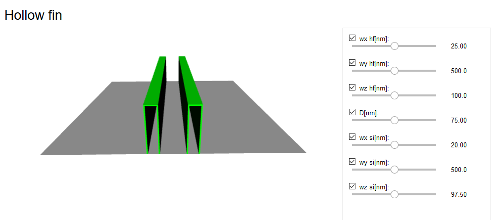
Figure 4: Widget for potential shape. Example with hollow fin.

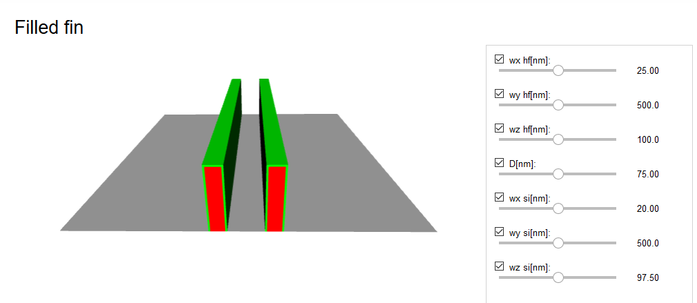
Figure 5: Widget for potential shape. Example with filled fin.

2.4.7 Structured samples. Small Angle Scattering

In previous section we described by means of potential our structure unit which consist of two Si fins covered with hafnium oxide. In this section we are going to use the created potential object for calculation of three-dimensional Small Angle Scattering pattern from a regular one-dimensional lattice of such fins. For this purpose we add a description of the lattice as following

⬇

latx = esc.lattice("", qx, T, 5)

show(latx, coordinates=np.linspace(-0.1, 0.1, 500),

xlabel="Qx")

The latx object is a one-dimensional functor which returns result for the lattice function of the following form

$$L(q_{x})=\left|\frac{\sin(Nq_{x}T0.5)}{\sin(q_{x}T0.5)}\right|^{2}$$ (7)

where $N$ - number of structure units in the lattice, which we have set as $N=5$. The resulted functor is depicted in figure 6

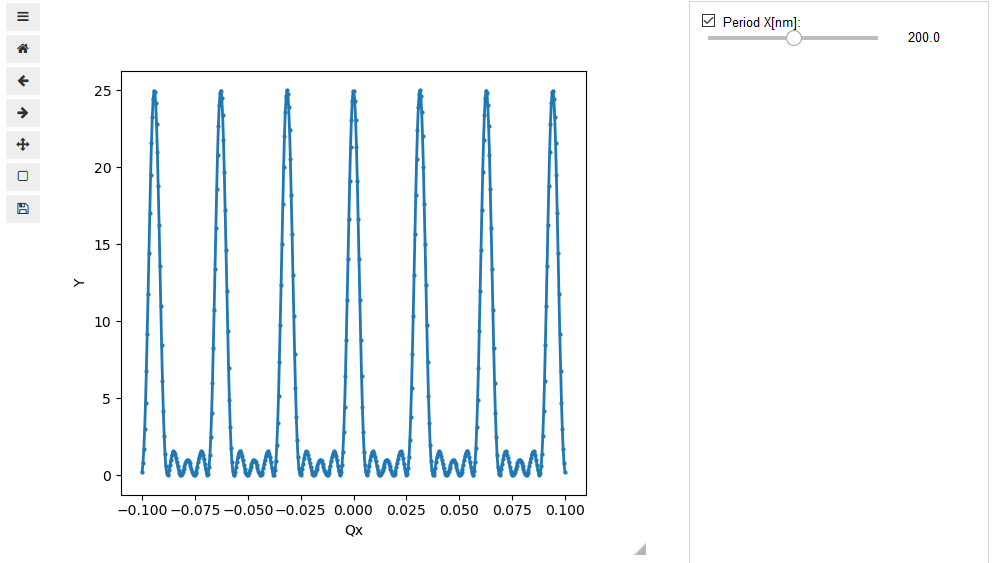
Figure 6: Widget for lattice functor.

Since latx is a functor, if equation 7 doesn’t satisfy the current needs, any other custom functor can be used instead. The two-dimensional lattice is also quite simple to implement, user has to create the second lattice functor along another axis, for example $q_{y}$, and simply multiply both latx*laty. The resulted functor correspond to the two-dimensional lattice along $q_{x}$ and $q_{y}$ axes.

In the next code listing we demonstrate how to create a functor which calculates Small Angle Scattering intensity. In addition to three variables, which correspond to scattering vector components $q_{x},\;q_{y},\;q_{z}$, it requires potential object and lattice as a functor of one or several variables.

⬇

show(I, coordinates=c, cblog=True,

cbmin=1, rows=sz,

plot_type="map", xlabel="Qx", ylabel="Qy")

The result of show command is depicted in figure 7.

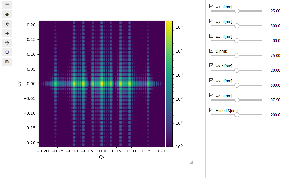
Figure 7: Calculated small angle scattering pattern.

3 Conclusion and outlook

In this article we presented the key features of the first public release, version 0.9.0, of ESCAPE software project. It took quite a lot of time to analyse advantages and disadvantages of existing scattering software, including commercial packages, and to find the best architecture for the core suitable for most of the scattering applications, balancing between experienced and non-experienced users. We believe that our way of software design, way of working with the data analysis will find followers in the scattering community. The standard format of Jupyter notebooks should help users of ESCAPE to share their experience with others using our repository (check www.escape-app.net). Below we give an outlook of the future features of ESCAPE.

3.1 Potential module and structured samples

Right now we are concentrated on further development of potential module, which we briefly described in section 2.4.6. The potential object supports simple arithmetic operations, allowing to create complicated shapes, forming a structure unit and to position them, defining their coordinates as independent fit parameters. Our users can operate with predefined existing shapes, use geometry object for creation of complex shapes based on simple shapes, or describe fully custom shape providing vertices coordinates. Each component of vertices coordinates is a parameter and user can easily link them to physical parameters of the described shape if necessary.

Currently, there is no control for shape overlapping, it is up to the user to check the correctness of parameters boundaries. We plan to add overlapping control in the next release together with the support for structured layers, necessary for GISAS and off-specular reflectivity applications.

3.2 Off-specular applications

The potential module will be the basis for new off-specular scattering functors. One can split the off-specular scattering applications on two branches: grazing incidence cases, like grazing incidence small angle scattering, grazing incidence diffraction, off-specular reflectometry and non-grazing cases, like 2D intensity maps of high resolution X-ray diffraction. The former types are not very popular in industrial applications due to the large footprint of an incident beam on the sample, but the latter one is used intensively for structured samples. The basis for these applications is already implemented in HRXRD and specular reflectivity modules. The objects for sample description for these cases do not require any significant update. We plan to implement them using kinematic, semi-kinematic and dynamic approximations.

3.3 Small angle scattering. Diluted samples

It is currently unclear for us whether we need a special module for small angle scattering for diluted samples. In our examples we have demonstrated that experiments can be simulated using only the core package. The development of this branch could go into two directions: adding more example notebooks covering most of the usual form-factors and user cases or adding these typical form-factors to the C++ core, which will certainly make calculation faster, but will reduce possibilities for customization. A more complicated cases could arise from the particles of complex shapes where the analytical expression of the form-factor can be quite difficult to achieve. Here the potential and geometry modules could help, especially if the same probes have been measured with conventional small angle scattering and GISAS. In this case the characteristic parameters of the particles could be shared between models and simultaneous fit performed. We leave this decision for the future community right now.

3.4 Acknowledgements

We thank Yury Khaydukov for providing experimental data for testing and performing first in situ tests and Miguel Castro-Collin for early testing, discussions and for his helpful feedback. Special thanks to Oleg Khoruzhiy for discussion about neural networks and useful references.