Fast radio bursts: do repeaters and non-repeaters originate in statistically similar ensembles?

Abstract

Fast Radio Bursts (FRBs) are the short, strong radio pulses lasting several milliseconds. They are subsequently identified, for the most part, as emanating from unknown objects at cosmological distances. At present, over one hundred FRBs have been verified, classified into two groups: repeating bursts (20 samples) and apparently non-repeating bursts (91 samples). Their origins, however, are still hotly debated. Here, we investigate the statistical classifications for the two groups of samples to see if the non-repeating and repeating FRBs have different origins by employing Anderson-Darling (A-D) test and Mann-Whitney-Wilcoxon (M-W-W) test. Firstly, by taking the pulse width as a statistical variant, we found that the repeating samples do not follow the Gaussian statistics (may belong to a $\chi$-square distribution), although the overall data and non-repeating group do follow the Gaussian. Meanwhile, to investigate the statistical differences between the two groups, we turn to M-W-W test and notice that the two distributions have different origins. Secondly, we consider the FRB radio luminosity as a statistical variant, and find that both groups of samples can be regarded as the Gaussian distributions under the A-D test, although they have different origins according to M-W-W tests. Therefore, statistically, we can conclude that our classifications of both repeaters and non-repeaters are plausible, that the two FRB classes have different origins, or each has experienced distinctive phases or been subject to its own physical processes.

1 Introduction

Fast radio bursts (FRBs) are bright, millisecond-duration radio pulses that generated from the extragalactic sources (in most cases) according to the dispersion measures (DM) and the redshift of host galaxies of localized FRBs (Lorimer et al., 2007; Thornton et al., 2013; Chatterjee et al., 2017). Great progresses have been made in observations and theories, since the first reported FRB in 2007 (Cordes & Chatterjee, 2019; Petroff, Hessels & Lorimer, 2019). More than one hundred of FRBs have been verified, 20 (91) of which are reported as repeating (apparently non-repeating) FRBs (Petroff et al., 2016; CHIME/FRB Collaboration et al., 2019a; Kumar et al., 2019; CHIME/FRB Collaboration et al., 2019b; Fonseca et al., 2020). The corresponding FRB detection rate is $\sim 10^{3}-10^{4}\rm{day^{-1}sky^{-1}}$ (Thornton et al., 2013; Spitler et al., 2014; Keane & Petroff, 2015; Rane et al., 2016; Oppermann, Connor & Pen, 2016; Champion et al., 2016; Scholz et al., 2016; Lawrence et al., 2017; Patel et al., 2018; Connor, 2019). The physical origin of FRBs is still unclear, though many theoretical models are proposed to solve this challenge (Cordes & Chatterjee, 2019; Petroff, Hessels & Lorimer, 2019), including the mergers of compact objects (Yamasaki, Totani & Kiuchi, 2018), collapse of supermassive neutron stars (Falcke & Rezzolla, 2014), energetic flares coming form the magnetars (Kulkarni et al., 2014; Connor, Pen & Oppermann, 2016; Cordes & Wasserman, 2016a; Popov & Pshirkov, 2016; Margalit & Metzger, 2018) and interactions between superconducting cosmic strings (Yu et al., 2014; Thompson, 2017).

Recently, bright millisecond-timescale radio bursts from the magnetar SGR 1935 + 2154 have been detected by CHIME/FRB (Scholz & Chime/Frb Collaboration, 2020) and STARE2 (Bochenek et al., 2020a). This phenomenon suggests that some FRBs may be involved in the strong magnetic activity generated by magnetars (Katz, 2016; Margalit et al., 2020; Andersen et al., 2020; Lin et al., 2020; Bochenek et al., 2020b; Lyutikov & Popov, 2020), especially for the repeating FRBs. The repeaters and apparently non-repeaters (hereafter referred to as non-repeaters) may have different physical origins. Thus, it is important to classify the FRBs based on the observed properties.

Clearly, it is natural to divide FRBs into two groups as repeating and non-repeating samples (Petroff, Hessels & Lorimer, 2019). Both pulse width and radio luminosity are important characteristics for FRBs and their radiative properties, and these are frequently used as FRB sorting criteria (Oppermann, Connor & Pen, 2016; Ravi, 2019; Qiu et al., 2020; Fonseca et al., 2020). Petroff, Hessels & Lorimer (2019) presented the histogram of FRB pulse width, however further statistical tests were not pursued. Recent results from the CHIME/FRB collaboration show that the distributions of two categories are not same with $\sim 5\sigma$ and $\sim 4\sigma$ significance using analysis of their own data on 18 repeating FRBs and 12 non-repeating ones (Fonseca et al., 2020). The ASKAP group found that the distribution of pulse width may not be bimodal (Qiu et al., 2020). But considering that the ASKAP sample is small and Bayesian methods are more suitable for large samples, the conclusion is still inconclusive. Meanwhile, much research on the radio luminosity of FRBs have been carried out, which mainly focuses on the luminosity function (Kumar, Lu & Bhattacharya, 2017; Luo et al., 2018, 2020; Hashimoto et al., 2020) , and radio spectrum (Spitler et al., 2016; Macquart et al., 2019; Katz et al., 2020). Although the above analyses are impressive, the statistics combined with more data from other telescopes and quantitative statistical tests are still needed.

Here, we collect all detected FRB data, including the information on pulse width and radio luminosity, to examine their distributions for the repeating and non-repeating samples and check whether two groups of samples have the same or different origins. In section 2, we organize and check the rationality of the data. In section 3, we exploit the Anderson-Darling (A-D) test to see whether the above data conform to the Gaussian distribution and use a Mann-Whitney-Wilcoxon (M-W-W) test to check whether the two distributions share the same origins. Finally, in section 4 we summarize our results, and discuss possible mechanisms for the repeating and non-repeating FRBs.

2 FRB Observation Data

Our data of FRBs are taken from the database of FRB Catalogue(FRBCAT) (Petroff et al., 2016), and those for repeating FRBs come from FRBCAT and published papers (Petroff et al., 2016; CHIME/FRB Collaboration et al., 2019a; Kumar et al., 2019; CHIME/FRB Collaboration et al., 2019b; Fonseca et al., 2020). According to FRBCAT, there is a significant gap between $\sim 35\,\rm{ms}$ and $\sim 300\,\rm{ms}$ in pulse width. However, we notice that the measurements with pulse width larger than $\sim 300\,\rm{ms}$ all come from one radio facility, i.e., the radio telescope BSA LPI of the Pushchino Radio Astronomy Observatory, in which the time interval between samples is $100\,\rm{ms}$ (Fedorova & Rodin, 2019). Considering that there may exist some observational bias effects in these data, we only include the pulses with a width shorter than $\sim 35\,\rm{ms}$ (80 non-repeaters). For non-repeating FRBs, the possibility of repetition cannot be rejected, in particular repeating signals from FRB171019 have been observed (Kumar et al., 2019) in 2019. However, our analysis is based on the current observational data, and the phenomenon of repeating signals in non-repeaters is difficult to predict at present. Therefore, we treat the apparently non-repeating sources as real non-repeaters under current circumstances. For repeating FRBs, two or more observations are included. Thus, we calculate the average pulse width and radio luminosity of each source as representative of its pulse width and radio luminosity, respectively. Since the pulse width in the FRBCAT is the observed width, which is easily affected by dispersion(Ravi, 2019), to study the pulse width more accurately, we need to introduce the intrinsic width that is estimated by Eq.(1) (Connor, Miller, & Gardenier, 2020; Qiu et al., 2020).

$$\begin{split}t_{i}=\sqrt{t_{obs}^{2}-t_{DM}^{2}-t_{s}^{2}}\end{split}$$ (1)

In the above formula, $t_{i}$ ($t_{obs}$) is the intrinsic width (observed width), with $t_{s}$ being the sampling time that depends on the instrument, and $t_{DM}$ is the dispersion smearing timescale as calculated in the following,

$$\begin{split}t_{DM}=8.3\times 10^{-3}\rm{DM{\Delta{\nu_{MHz}}\over\nu_{GHz}^{3}}\quad ms}\end{split}$$ (2)

where $\rm DM$ is the dispersion measure, $\rm\Delta{\nu_{MHz}}$ is the channel bandwidth in the unit of MHz and $\nu_{\rm GHz}$ is the central frequency in the unit of GHz. Therefore, the pulse width in the following text represents the intrinsic width. In Table 1, we summarize the properties of 20 repeating FRBs, by listing the observed width, intrinsic width, flux density, fluence and luminosity distance. In Figure 1, we plot a histogram of the pulse width for the repeating and non-repeating FRBs.

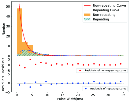
Figure 1: Upper panel: histogram of repeating and non-repeating FRBs with pulse width $<35\,\rm{ms}$. The solid (dashed) line is the fitted curve for non-repeating (repeating) FRBs. The filled histogram is for non-repeating FRBs and the cross-hatched histogram is for repeating FRBs. Middle and bottom panels: the residuals for the non-repeaters and repeaters between the source data and fitted curve, shown as solid points, where the dashed lines refer to the cases of residual=0.

3 FRB Classifications and Statistical Tests

3.1 Samples of all FRBs

A Gaussian distribution occurs naturally in many astronomical data sets (Press, Flannery, & Teukolsky, 1986; Mackay, 2003), sometimes occurring in data with logarithmic sampling. For completeness, we first investigate the Gaussian property. Regarding the total statistical properties of all FRBs, if we assume that the pulse widths of these data follow the Gaussian distribution, we can apply the A-D test (Ivezić et al., 2019) to examine whether the assumption is correct. The results of A-D test are shown in Table 2. For a 0.05 significance level, the statistic (0.547) is smaller than the critical value (0.760), which indicates that the Gaussian property of the data on pulse width is probable. We further use the A-D test to examine whether the radio luminosity of FRBs conforms to a Gaussian distribution, and the result shows that its statistic (0.475) is smaller than the critical value (0.759, as seen in Table 2), which means that the Gaussian property of the radio luminosity is likely. Therefore, using a Gaussian distribution to fit for the pulse width and radio luminosity is acceptable for all data but unknown for the separate data. Next we will discuss the distributions for the two samples of repeaters and non-repeaters.

Table 1: Parameters of 20 repeating FRBs. ^a

No.	Sources	Observed Widthb	Intrinsic Widthc	Flux Densityd	Fluencee	Distancef	Refs.
		(ms)	(ms)	(Jy)	(Jy ms)	(Gpc)
1	FRB121102	4.82	4.78	0.25	0.372	1.61	(1)
2	FRB180814.J0422+73	23.45(22.57)g	23.43	…h	22.57	0.39	(2)(3)
3	FRB171019	4.62	4.08	…hi	101.54	1.89	(4)
4	FRB180916.J0158+65	5.27	5.16	2.08	1.62	0.58	(5)
5	FRB181030.J1054+73	1.01	0.10	3.15	4.75	0.24	(5)
6	FRB181128.J0456+63	5.90	5.80	0.40	3.45	1.14	(5)
7	FRB181119.J12+65	3.49	3.33	0.43	1.77	1.42	(5)
8	FRB190116.J1249+27	2.75	2.53	0.35	1.80	1.90	(5)
9	FRB181017.J1705+68	16.8	16.73	0.40	8.50	6.97	(5)
10	FRB190209.J0937+77	6.55	6.46	0.50	1.25	1.66	(5)
11	FRB190222.J2052+69	2.71	2.48	1.65	5.45	1.64	(5)
12	FRB190208.J1855+46	1.11	0.14	0.50	1.70	2.35	(6)
13	FRB180908.J1232+74	3.83	3.70	2.90	0.50	0.62	(6)
14	FRB190604.J1435+53	2.10	1.78	0.75	8.30	2.42	(6)
15	FRB190212.J18+81	3.10	2.93	0.75	2.75	1.05	(6)
16	FRB190303.J1353+48	3.20	3.04	0.47	2.67	0.77	(6)
17	FRB190417.J1939+59	4.50	4.20	0.53	3.10	7.40	(6)
18	FRB190117.J2207+17	2.74	2.53	1.00	6.36	1.49	(6)
19	FRB190213.J02+20	7.00	6.90	0.50	1.80	2.91	(6)
20	FRB190907.J08+46	2.18	1.92	0.30	2.03	1.07	(6)

^a The highest radio luminosity is $1.2\times 10^{44}\,\rm{erg/s}$ from FRB190523, and the faintest for extragalactic conditions is $6.2\times 10^{38}\,\rm{erg/s}$ from FRB141113. ^b The average observed width. ^c The average intrinsic width calculated by eq.(1). ^d The average flux density. ^e The average fluence. ^f The distance is from FRBCAT (Wright, 2006) based on $\rm{\Lambda CDM}$ with cosmological parameters: $\rm{H_{0}=69.6\,km/s/Mpc}$, $\rm{\Omega_{M}=0.286}$ and $\rm{\Omega_{vac}=0.714}$, where $\rm{H_{0}}$ is Hubble constant, $\rm{\Omega_{M}}$ is the mass fraction in the universe and $\rm{\Omega_{vac}}$ is the dark energy fraction in the universe. ^g 23.45 is from CHIME (CHIME/FRB Collaboration et al., 2019a), while 22.57 is from FRBCAT. In our statistics we use the data from CHIME. ^h The parameters are not given in FRBCAT or Refs.. ⁱ The flux density is not given, but the fluence is given. So we use the fluence to estimate the luminosity.

Refs. : (1) Spitler et al. (2016); (2) CHIME/FRB Collaboration et al. (2019a); (3) FRBCAT; (4) Kumar et al. (2019); (5) CHIME/FRB Collaboration et al. (2019b); (6) Fonseca et al. (2020).

3.2 Samples of repeating and non-repeating FRBs

To obtain the statistical test results for FRB classifications, we can apply the A-D test and M-W-W test. Here, due to the small size of repeater sample (20 repeating FRBs), a Kolmogorov-Smirnov (K-S) test is not an effective tool (Ivezić et al., 2019; Yang et al., 2019). For example, for a sample size of 10, the error of a K-S test can reach 7%. Thus, we adopt the A-D test to check whether the sample distribution is consistent with a single Gaussian, then use the M-W-W test to examine whether the two samples share the same origin even if the data volumes are different. In our case, the two groups of samples for repeating and non-repeating FRBs are tested, based on the two characteristic quantities, the pulse width and radio luminosity. On the one hand, according to the data in Table 1, there are 20 repeaters, the pulse width of which range from $\sim 0.1\,\rm{ms}$ to $\sim 23\,\rm{ms}$. On the other hand, for the non-repeating FRB data, the pulse widths range from $\sim 0.05\,\rm{ms}$ to $\sim 34\,\rm{ms}$. The mean pulse width of repeating (non-repeating) sources is $\sim 5.10\,\rm{ms}$ ($\sim 3.35\,\rm{ms}$). We use A-D test to check the Gaussian property of both groups of samples, the results of which are shown in Table 2.

The results show that the distribution of pulse width for repeating samples is not Gaussian in either logarithmic or linear coordinates scales, while the non-repeating sample belongs to a Gaussian distribution if expressed logarithmically. Furthermore, to check if the distribution of repeating FRB pulse widths follows a $\chi$-square type in linear coordinates, the function of which can be described below,

$$\begin{split}f_{k}(x)&={1\over 2^{{k/2}}\Gamma({k/2})}x^{k/2-1}e^{-x/2}\\ &=Ax^{k/2-1}e^{-x/2}\ \end{split}$$ (3)

where A is referred as the fitting coefficient. Here we employ Eq. (3) to fit the pulse width data of repeaters with the best fitting parameters of $\rm A=72.978$ and $\rm k=1.626$. The goodness of the $\chi$-square fit is calculated by Eq. (4) and the result is 0.80. In Eq. (4), $R^{2}$ is the goodness of fit, RSS is residual sum of the square, TSS is the total sum of squares, $y_{i}$ values are real data, $\hat{y}$ are test data on the fitted curve and $\overline{y}$ is mean value of the real data. Through the Figure 1, the histograms are all on the fitted curve or on both sides of the curve. Thus, we conclude that the distribution of pulse widths of repeating FRBs could follow a $\chi$-square function.

$$\begin{split}R^{2}&=1-RSS/TSS\\ &=1-\sum\limits_{i=1}^{n}(y_{i}-\hat{y})^{2}/\sum\limits_{i=1}^{n}(y_{i}-\overline{y})^{2}\end{split}$$ (4)

In Figure2, we draw the cumulative distribution function (CDF) for the two groups of samples. Although the two CDFs are close to each other, they belong to different distributions. To evaluate the reliability of above inference, we apply a M-W-W test. The resulting p-value of this M-W-W test is 0.0065, which is less than 0.05, indicating that the distribution of two groups are different, as shown in Table 3.

As a next step, we try to use the radio luminosity as a statistical variant to realize classification for two group samples. The radio luminosity is estimated by Eq. (5), where S is the flux density and D is the luminosity distance.

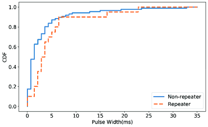
Figure 2: Cumulative distribution function (CDF) of pulse width. The dashed line is for repeating FRBs, the solid line is for non-repeating FRBs.

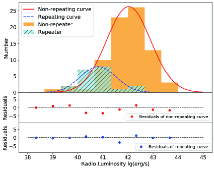
Figure 3: Histogram of repeating and non-repeating FRBs for radio luminosity expressed logarithmically. The solid line is the fitted curve of non-repeating FRBs. The dashed line is the fitted curve of repeating FRBs. The cross-hatched histogram is repeating FRBs and the empty one means non-repeating FRBs. Middle and bottom panels: the residuals for the non-repeaters and repeaters between the source data and fitted curve, shown as solid points, where the dashed lines refer to the cases of residual=0.

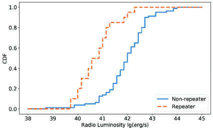
Figure 4: Cumulative distribution function (CDF) of radio luminosity. The dashed line is for repeating FRBs and the soild one shows the non-repeating FRBs.

$$\begin{split}L_{\rm{radio}}\sim SD^{2}\ \end{split}$$ (5)

First of all, the radio luminosity of repeaters and non-repeaters ranges from $\sim 10^{39}\,\rm{erg/s}$ to $\sim 10^{42}\,\rm{erg/s}$ and $\sim 10^{38}\,\rm{erg/s}$ to $\sim 10^{44}\,\rm{erg/s}$, respectively. We plot their histograms in Figure 3. The mean radio luminosity of repeating (non-repeating) sources is $\sim 2.6\times 10^{41}\,\rm{erg/s}$ ($\sim 6.2\times 10^{42}\,\rm{erg/s}$). Then, we need to test for the Gaussian property of the repeating and non-repeating groups by using A-D test, the results of which are shown in Table 2: for the repeating FRBs the statistic (0.333) is smaller than the critical value (0.692), and for the non-repeating FRBs the statistic (0.592) is also smaller than the critical value (0.752), so they are both under the corresponding significance level of 0.05. Hence, these results indicate that the distributions of two groups conform to Gaussian distributions. In Figure 4, we draw the CDF for two groups, finding that the two curves are well-separated. We find both distributions are different using the M-W-W test, for which p-value is $7.905\times 10^{-7}$, much smaller than 0.05, as shown in Table 3. In short, from the viewpoint of statistical tests, two groups of samples very likely have different distributions.

Table 2: A-D test to check Gaussian property ^a.

Sample	Statistic b	Critical values ($\alpha=0.05$)c
Pulse Width
All Data	0.547	0.760
Non-repeating	0.692	0.754
Repeating	1.430	0.692
Luminosity
All Data	0.475	0.759
Non-repeating	0.592	0.752
Repeating	0.333	0.692

^a Tested when in logarithmic scale.

^b The statistic in the A-D test. Only when it is smaller than a critical value does the result make sense;

^c The significance level in A-D test we take to be 0.05.

Table 3: M-W-W test to check different distributions.

Characteristic					P-values
Pulse Width					0.0065
Radio Luminosity					$7.905\times 10^{-7}$
Radio Luminosity in CHIME Data					$8.79\times 10^{-6}$
Adjusted Radio Luminosity					$2.47\times 10^{-9}$

However, we notice that the mean values of radio luminosity for non-repeaters are different for the CHIME data with central frequency of 600MHz ($\rm{1.77\times 10^{43}\,erg/s}$) and other data centered around 1.4GHz ($\rm{2.59\times 10^{42}\,erg/s}$) (Luo et al., 2020). If we assume that the detected FRBs by both the CHIME and other radio telescopes are originated from the same phenomenon, then the two mean values of luminosity should be similar in the case of readjusting the observational frequency. In other words, the two different mean values of luminosity of FRBs by the different instruments may be caused by the observation frequency bands or facilities calibration. First, we simply use the CHIME data (Fonseca et al., 2020) with 18 repeaters and 12 non-repeaters to test the former conclusion, whether the two samples have the same distributions. Through M-W-W test, the p-value is $8.79\times 10^{-6}$ which is consistent with the former conclusion that they follow the different origins statistically. Second, we shift the luminosity values of CHIME by reducing an order of magnitude, which results in the same mean value as that by the other telescopes, as shown in Figure 5. Obviously, the two samples of the adjusted non-repeaters and repeaters are tested by applying M-W-W test, as shown in Table 3, and the result shows the same conclusion as the former that the repeaters and non-repeaters belong to the different distributions.

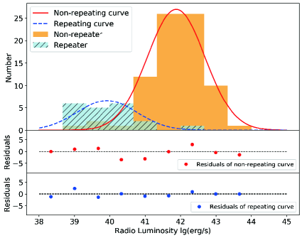
Figure 5: Histogram of repeating and non-repeating FRBs for radio luminosity on a logarithmic scale, after the adjustment of data. The solid (dashed) line stands for the fitted curve of non-repeating (repeating) FRBs. The cross-hatched histogram is for repeating FRBs and the empty histogram means the non-repeating ones. Middle and bottom panels: residuals of non-repeaters and repeaters between source data and the fitted curve, shown as solid points. Dashed lines refer to residual=0.

4 Conclusions and Discussions

In this paper, we employ statistical methods to analyze the distributions of FRB properties based on the statistical variants of FRB pulse width and radio luminosity, in an attempt to classify the two sample groups, the repeating (20 samples) and non-repeating (80 samples) bursts. Because of the small FRB sample sets at present, we avoid the K-S test and employ the M-W-W test due to larger uncertainties of the former. We find that the two groups of samples have different origins, with the significance level of 0.05.

We think that the statistical classification turns out to be an effective guide to understanding FRB origins. Firstly, taking the pulse width as a statistical variant, the distribution of non-repeating group is conforms to a Gaussian, but a Gaussian property for the repeating group is not clear ($\chi$-square distribution seems to be better) when an A-D test is applied. Furthermore, using M-W-W test, we find that the distributions of two groups, repeating and non-repeating, are different. Secondly, in terms of radio luminosity, by adopting the A-D test, we find that the distributions of repeating and non-repeating groups are both Gaussian. A further M-W-W test shows that the distributions of two groups are significantly different. In addition, for a more complete conclusion, we notice that the CHIME data present the FRB luminosity of non-repeaters one order of magnitude higher than that of the other telescopes, in average. Again, we adjust the CHIME data by reducing one order of magnitude to test if the modified data of CHIME repeaters has the different origin from the non-repeaters, and we obtained the same conclusion as that for the unadjusted data by M-W-W test: non-repeaters and repeaters have the different origins. Therefore the statistical difference between two samples of data indicates that they may have a different physical origin, or the repeating and non-repeating phenomena originates in very different physical processes.

There are some interpretations concerning our data and conclusion which need to be clarified. 1) The pulse width data from FRBCAT is the observed value and further obtained by search code (Petroff et al., 2016), but it is not the intrinsic width. Moreover, according to papers published by CHIME (CHIME/FRB Collaboration et al., 2019b) and Kumar et al. (2019), the data they present have been fitted with Gaussian profiles, which means that these data are the observed pulse width. Since the main purpose of this paper is not to discuss the DM-t relationship, we directly use the Eq.(1) to estimate the intrinsic width. Thus, for these data, we do not apply further processing to remove the additional intrinsic structure effects. 2) The pulse width and flux density data are not corrected precisely for frequency, because the spectral index of each FRB is difficult to determine, in particular for the lack of data for simultaneous observation of the same source at different frequencies. 3) The distance we use is from FRBCAT (Wright, 2006) based on $\rm{\Lambda CDM}$ with cosmological parameters: $\rm{H_{0}=69.6\,km/s/Mpc}$, $\rm{\Omega_{M}=0.286}$ and $\rm{\Omega_{vac}=0.714}$. Some papers on luminosity function, such as the work by Luo et al.(Luo et al., 2020), use $\rm{\Lambda CDM}$ with cosmological parameters: $\rm{H_{0}=67.8\,km/s/Mpc}$, $\rm{\Omega_{M}=0.308}$ and $\rm{\Omega_{vac}=0.692}$. 4) The goodness of repeaters’ pulse width fitting curve is only 0.80, which is not high enough. This indicates that even though the distribution of repeaters’ pulse width is not the Gaussian, the $\chi$-square type should be not the best. The explanation for this may be due to the lack of observation data.

To explain the physical origins of repeating and non-repeating FRB mechanisms, many FRB models have been proposed. Now that we find two ”congenital” origins related to different physical processes, the two camps of models will be briefly summarized. In general, FRB models usually involve the physical processes of compact objects [white dwarf (WD), neutron star (NS), black hole (BH)], or the medium around them. Repeating FRB models usually relate to the interaction of compact objects with companion stars or the surrounding medium, including the super giant pulses from young NS or pulsars (Cordes & Wasserman, 2016a; Connor, Pen & Oppermann, 2016), extreme activities in the magnetosphere magnetars (Kulkarni et al., 2014; Wang, Xu & Chen, 2020; Lyutikov & Popov, 2020), accretion of compact objects (Gu et al., 2016), NS interaction with comets or asteroids (Dai et al., 2016), and maser phenomenon in the surrounding medium of magnetars (Yu et al., 2020). For the non-repeating FRBs, many models involve the one-off explosive events such as the mergers of compact object binaries or collisions between one compact object and another astronomical object, for example, mergers of BH-NS (Zhang, 2016), NS-NS (Yamasaki, Totani & Kiuchi, 2018), WD-BH (Li et al., 2018), or comets and asteroid hitting the surface of a NS (Geng & Huang, 2015).

Because our statistical results support the classification of FRB into repeating and non-repeating categories, our work puts certain constraints on the different models. For example, a model needs to be discussed from the perspective of repeating and non-repeating, especially the luminosity difference between repeaters and non-repeaters is about 1.5 orders of magnitude. This difference may indicate that the non-repeating sources come from a onetime catastrophic energy release or a violent outburst with a long energy storage period.

Furthermore, compared with the latest results from CHIME (Fonseca et al., 2020) and Luo et al.(Luo et al., 2020), all data in FRBCAT have been considered and the new method of M-W-W test has been used in this work. However, we have to note that different observed center frequencies may cause the changes in pulse width and radio luminosity, which may be the reason why the former research did not consider all the data. Finally, long-term observations of the repeating sources will test the different models and give us a better understanding of their burst mechanisms. We hope that in terms of further observations, the same FRB can be observed at the different frequency bands simultaneously. In this way, we can more accurately determine the spectral index of FRBs, thereby constraining the luminosity function of FRBs. Many more FRBs are expected to be published soon from CHIME, ASKAP, and FAST (Li et al., 2018; Li, Dickey, & Liu, 2019; Zhu et al., 2020), the higher sensitivity of which could provide valuable information regarding their still mysterious origin.

Data Availability

The data underlying this article are available in the references below: (1) Spitler, et al. (2016); (2) CHIME/FRB Collaboration, et al. (2019a); (3) Kumar et al. (2019); (4) CHIME/FRB Collaboration, et al. (2019b); (5) Fonseca, et al. (2020). Some data of FRBs are taken from the database of FRB Catalogue (FRBCAT), available at http://www.frbcat.org/.

References

- Andersen et al. (2020) Andersen B. C., et al., 2020, arXiv, arXiv:2005.10324
- Bochenek et al. (2020a) Bochenek C., Kulkarni S., Ravi V., McKenna D., Hallinan G., Belov K., 2020, ATel, 13684, 1
- Bochenek et al. (2020b) Bochenek C. D., Ravi V., Belov K. V., Hallinan G., Kocz J., Kulkarni S. R., McKenna D. L., 2020, arXiv, arXiv:2005.10828
- Champion et al. (2016) Champion D. J., et al., 2016, MNRAS, 460, L30
- Chatterjee et al. (2017) Chatterjee S., Law C. J., Wharton R. S., Burke-Spolaor S., Hessels J. W. T., Bower G. C., Cordes J. M., et al., 2017, Natur, 541, 58. doi:10.1038/nature20797
- CHIME/FRB Collaboration et al. (2019a) CHIME/FRB Collaboration, et al., 2019, Nature, 566, 235
- CHIME/FRB Collaboration et al. (2019b) CHIME/FRB Collaboration, et al., 2019, ApJL, 885, L24
- Chime/Frb Collaboration et al. (2020) Chime/Frb Collaboration, et al., 2020, Nature, 582, 351
- Cho et al. (2020) Cho H., et al., 2020, ApJL, 891, L38
- Connor, Pen & Oppermann (2016) Connor L., Pen U.-L., Oppermann N., 2016, MNRAS, 458, L89
- Connor (2019) Connor L., 2019, MNRAS, 487, 5753
- Connor, Miller, & Gardenier (2020) Connor L., Miller M. C., Gardenier D. W., 2020, MNRAS, 497, 3076
- Cordes & Wasserman (2016a) Cordes J. M., Wasserman I., 2016, MNRAS, 457, 232
- Cordes et al. (2016b) Cordes J. M., Wharton R. S., Spitler L. G., Chatterjee S., Wasserman I., 2016, arXiv, arXiv:1605.05890
- Cordes & Chatterjee (2019) Cordes J. M., Chatterjee S., 2019, ARA&A, 57, 417
- Dai et al. (2016) Dai Z. G., Wang J. S., Wu X. F., Huang Y. F., 2016, ApJ, 829, 27
- Falcke & Rezzolla (2014) Falcke H., Rezzolla L., 2014, A&A, 562, A137
- Fedorova & Rodin (2019) Fedorova V. A., Rodin A. E., 2019, ARep, 63, 877
- Fonseca et al. (2020) Fonseca E., et al., 2020, ApJL, 891, L6
- Geng & Huang (2015) Geng J. J., Huang Y. F., 2015, ApJ, 809, 24
- Gu et al. (2016) Gu W.-M., Dong Y.-Z., Liu T., Ma R., Wang J., 2016, ApJL, 823, L28
- Katz (2016) Katz J. I., 2016, ApJ, 826, 226
- Katz et al. (2020) Katz A., Kopp J., Sibiryakov S., Xue W., 2020, MNRAS, 496, 564
- Hashimoto et al. (2020) Hashimoto T., et al., 2020, MNRAS, 494, 2886
- Ivezić et al. (2019) Ivezić Ž., Connelly A. J., Vanderplas J. T., Gray A., 2019, sdmm.book
- Keane & Petroff (2015) Keane E. F., Petroff E., 2015, MNRAS, 447, 2852
- Kulkarni et al. (2014) Kulkarni S. R., Ofek E. O., Neill J. D., Zheng Z., Juric M., 2014, ApJ, 797, 70
- Kumar, Lu & Bhattacharya (2017) Kumar P., Lu W., Bhattacharya M., 2017, MNRAS, 468, 2726
- Kumar et al. (2019) Kumar P., Shannon R. M., Osłowski S., Qiu H., Bhandari S., Farah W., Flynn C., et al., 2019, ApJL, 887, L30
- Lawrence et al. (2017) Lawrence E., Vander Wiel S., Law C., Burke Spolaor S., Bower G. C., 2017, AJ, 154, 117
- Li et al. (2018) Li L.-B., Huang Y.-F., Geng J.-J., Li B., 2018, RAA, 18, 061
- Li et al. (2018) Li D., Wang P., Qian L., Krco M., Jiang P., Yue Y., Jin C., et al., 2018, IMMag, 19, 112. doi:10.1109/MMM.2018.2802178
- Li, Dickey, & Liu (2019) Li D., Dickey J. M., Liu S., 2019, RAA, 19, 016. doi:10.1088/1674-4527/19/2/16
- Lin et al. (2020) Lin L., et al., 2020, arXiv, arXiv:2005.11479
- Lorimer et al. (2007) Lorimer D.R., Bailes M., McLaughlin M.A., Narkevic D.J., Crawford F., 2007, Science, 318, 777
- Lorimer et al. (2013) Lorimer D. R., Karastergiou A., McLaughlin M. A., Johnston S., 2013, MNRAS, 436, L5
- Luo et al. (2018) Luo R., Lee K., Lorimer D. R., Zhang B., 2018, MNRAS, 481, 2320
- Luo et al. (2020) Luo R., Men Y., Lee K., Wang W., Lorimer D. R., Zhang B., 2020, MNRAS, 494, 665
- Lyutikov & Popov (2020) Lyutikov M., Popov S., 2020, arXiv, arXiv:2005.05093
- Mackay (2003) Mackay D. J. C., 2003, itil.book, 640
- Macquart et al. (2019) Macquart J.-P., Shannon R. M., Bannister K. W., James C. W., Ekers R. D., Bunton J. D., 2019, ApJL, 872, L19
- Mahony et al. (2018) Mahony E. K., et al., 2018, ApJL, 867, L10
- Margalit & Metzger (2018) Margalit B., Metzger B. D., 2018, ApJL, 868, L4
- Margalit et al. (2020) Margalit B., Beniamini P., Sridhar N., Metzger B. D., 2020, arXiv, arXiv:2005.05283
- Oppermann, Connor & Pen (2016) Oppermann N., Connor L. D., Pen U.-L., 2016, MNRAS, 461, 984
- Patel et al. (2018) Patel C., et al., 2018, ApJ, 869, 181
- Petroff et al. (2016) Petroff E., et al., 2016, PASA, 33, e045
- Petroff, Hessels & Lorimer (2019) Petroff E., Hessels J. W. T., Lorimer D. R., 2019, A&ARv, 27, 4
- Popov & Pshirkov (2016) Popov S. B., Pshirkov M. S., 2016, MNRAS, 462, L16
- Press, Flannery, & Teukolsky (1986) Press W. H., Flannery B. P., Teukolsky S. A., 1986, nras.book
- Prochaska et al. (2019) Prochaska J. X., et al., 2019, Science, 366, 231
- Qiu et al. (2020) Qiu H., et al., 2020, arXiv, arXiv:2006.16502
- Rane et al. (2016) Rane A., Lorimer D. R., Bates S. D., McMann N., McLaughlin M. A., Rajwade K., 2016, MNRAS, 455, 2207
- Ravi (2019) Ravi V., 2019, NatAs, 3, 928
- Scholz et al. (2016) Scholz P., et al., 2016, ApJ, 833, 177
- Scholz & Chime/Frb Collaboration (2020) Scholz P., Chime/Frb Collaboration, 2020, ATel, 13681, 1
- Spitler et al. (2014) Spitler L. G., et al., 2014, ApJ, 790, 101
- Spitler et al. (2016) Spitler L. G., et al., 2016, Nature, 531, 202
- Thompson (2017) Thompson C., 2017, ApJ, 844, 65
- Thornton et al. (2013) Thornton D., Stappers B., Bailes M., Barsdell B., Bates S., Bhat N.D.R., Burgay M., Burke-Spolaor S., Champion D.J., Coster P., D’Amico N., Jameson A., Johnston S., Keith M., Kramer M., Levin L., Milia S., Ng C., Possenti A., van Straten W., 2013, Science, 341, 53
- Wang, Xu & Chen (2020) Wang W.-Y., Xu R., Chen X., 2020, arXiv, arXiv:2005.02100
- Wright (2006) Wright E. L., 2006, PASP, 118, 1711
- Yamasaki, Totani & Kiuchi (2018) Yamasaki S., Totani T., Kiuchi K., 2018, PASJ, 70, 39
- Yang et al. (2019) Yang Y.-Y., Zhang C.-M., Li D., Chen L., Linghu R.-F., Zhi Q.-J., 2019, PASP, 131, 064201
- Yu et al. (2014) Yu Y.-W., Cheng K.-S., Shiu G., Tye H., 2014, JCAP, 2014, 040
- Yu et al. (2020) Yu Y.-W., Zou Y.-C., Dai Z.-G., Yu W.-F., 2020, arXiv, arXiv:2006.00484
- Zhang (2016) Zhang B., 2016, ApJL, 827, L31
- Zheng et al. (2014) Zheng Z., Ofek E. O., Kulkarni S. R., Neill J. D., Juric M., 2014, ApJ, 797, 71
- Zhu et al. (2020) Zhu W., et al., 2020, ApJL, 895, L6