Uncovering Majorana nature through a precision measurement of $CP$ phase

Abstract

We show the possibility to discover the neutrino nature by measuring the Majorana CP phase at the DUNE experiment. This phase is turned on by a decoherence environment, possibly originated by physics at the Planck scale. A sizable distortion in the measurement of the Dirac CP violation phase $\delta_{\mathrm{CP}}$ is observed at DUNE when compared with T2HK measurement due to decoherence and non-null Majorana phase. Being that, when the measurement of the Majorana phase is performed at DUNE, it reaches a precision of 23 (21) $\%$ for a decoherence parameter $\Gamma=4.5(5.5)\times 10^{-24}\mathrm{GeV}$ and a Majorana phase equal to $1.5\pi$. The latter precision is similar to the one obtained at the T2K experiment at its current Dirac CP violation phase measurement.

I Introduction

The origin of neutrino masses is one of the most relevant questions of modern elementary particle physics Murayama:2006qb ; Valle:2015mma . The Standard Model (SM) Higgs mechanism could generate the neutrino masses if they were Dirac particles. However, this SM alternative does not explain why the neutrino masses are less than one-millionth of the electron’s mass, the smallest charged lepton. The general belief is that the latter is resolved through the seesaw mechanism, being the most inexpensive case when neutrinos are Majorana particles Yanagida:1979as ; GellMann:1980vs ; Glashow:1979nm ; Minkowski:1977sc ; Mohapatra:1979ia ; Magg:1980ut ; Schechter:1980gr ; Mohapatra:1980yp ; Foot:1988aq ; Shrock:1980ct ; Konetschny:1977bn ; Cheng:1980qt ; Lazarides:1980nt . The Majorana neutrinos, a fermion that is its own antiparticles, imply the total lepton charge violation, a conserved number within the SM processes Atre:2009rg ; Zee:1985id . Therefore, the quest for elucidating the Majorana nature of neutrinos is one of our best chances to learn about what is beyond the SM. The usual way to look for Majorana neutrinos is using the neutrinoless double beta decay, a lepton charge violating process not allowed by the SM Faessler:1999zg ; Avignone:2007fu ; Vergados:2012xy ; Bilenky:2012qi . Until now, there is no signal from the latter Agostini:2019hzm ; Anton:2019wmi ; Adams:2019jhp ; KamLAND-Zen:2016pfg or other proposes way of searches for Majorana neutrinos Sirunyan:2018xiv ; Aaij:2014aba ; Balantekin:2018ukw ; Bora:2016ygl .

The standard oscillation neutrino (SO) probabilities take the same form regardless of the neutrino nature. Only the Dirac CP phase is observable while the two other CP violation phases, when the neutrino is Majorana, are absorbed Giunti:2010ec . However, if we suppose a new physics(NP) phenomenon, subleading to the SO mechanism, exists, the latter situation could be no longer valid. Therefore, this NP could help the Majorana phases to emerge in the oscillation probabilities. The NP phenomena we focus on forecasts an interaction between the neutrino system with the environment at the Planck scale level, which is characterized by a foamy space-time Benatti:2000ph . The loss of quantum coherence (decoherence) in the neutrino system is the interaction’s main signature. The foamy space-time is predicted in the context of strings and branes Ellis:1992eh ; Ellis:1992pm ; Benatti:1998vu , and quantum gravity Hawking:1982dj . This quantum decoherence phenomena in the neutrino system have been vastly studied in the literature Lisi:2000zt ; Barenboim:2006xt ; Bakhti:2015dca ; Carpio:2017nui ; Carpio:2018gum ; Gomes:2020muc wherein most of the cases containing only the damping effects. Nevertheless, the phenomenology of the interaction between neutrino and a quantum decoherence environment goes beyond the damping effects, being that this might add new contributions to the violation of CP or CPT deOliveira:2013dia , Capolupo:2018hrp and Carrasco:2018sca . Through these kinds of contributions in the neutrino oscillation formula, we can reveal the neutrino’s Majorana nature. The observability of the Majorana nature using neutrino oscillation is a rather novel approach.

At this point it is worth mentioning that our work’s cornerstone hypothesis is that the Dirac CP violation phase measured at T2K experiment represents its real value since it is unaffected by quantum decoherence in neutrino oscillations. Thus, considering that the effects of a quantum decoherence environment, coupled with a non zero Majorana phase, are sizable in the DUNE data, our strategy is divided into two steps. The first step is to assess how much a measurement at DUNE experiment Acciarri:2015uup of the Dirac CP violation phase can deviate from the true one. For this purpose, and taking the pure SO as a theoretical hypothesis in the fitting, the CP violation phase obtained at DUNE is compared with the projected one at the T2HK experiment Abe:2018uyc . The T2HK projected measurement comes to be an upgrade in the precision of the CP violation measurement at T2K. The second step, and final goal in this letter, is to go beyond testing the DUNE accuracy for determining a Majorana CP phase simultaneously with the decoherence parameter.

II General Theoretical Formalism

The treatment for a neutrino subsystem embodied in an infinity unknown reservoir or environment, with which the former interacts weakly, can be obtained by the Lindblad Master equation Benatti:2000ph :

$$\frac{\partial\rho(t)}{\partial t}=-i[H,\rho(t)]+\mathcal{D}[\rho(t)],$$ (1)

where $\rho(t)$ is the reduced (neutrino) density matrix, obtained after trace over the degrees of freedom of the environment, $H$ is the Hamiltonian of the neutrino subsystem and $\mathcal{D}[\rho(t)]$ is the dissipative term which encloses the decoherence phenomena. The aforementioned factor can be written as $\mathcal{D}[\rho(t)]=\frac{1}{2}\sum_{j}\left([A_{j},\rho(t)A_{j}^{\dagger}]+[A_{j}\rho(t),A_{j}^{\dagger}]\right)$. Thus, if we work in a three-level system the operators $\rho$, $H$ and $A_{j}$ can be written as follows: $\rho=\sum\rho_{\mu}t_{\mu}$, $H=\sum h_{\mu}t_{\mu}$, and $A_{j}=\sum a^{j}_{\mu}t_{\mu}$ where $\mu$ is running from 0 to 8, $t_{0}$ is the identity matrix and $t_{k}$ the Gell-Mann matrices $(k=1,...,8)$ that satisfy $[t_{a},t_{b}]=i\sum_{c}f_{abc}t_{c}$, where $f_{abc}$ are the structure constants of $SU(3)$. The hermiticity of $\hat{A}_{j}$, which is secured demanding a time-increase Von Neumman entropy, allow us to write a symmetric $\bf{D}\equiv$ $D_{kj}$ dissipative/decoherence matrix as: $D_{kj}=\frac{1}{2}\sum_{l,m,n}(a_{nl})f_{knm}f_{mlj}$, where $a_{nl}=\vec{a}_{n}.\vec{a}_{l}$ with components $D_{\mu 0}=D_{0\mu}=0$, and $\vec{a}_{r}=\{a^{1}_{r},a^{2}_{r},...,a^{8}_{r}\}$. The matrix $\bf{A}\equiv$ $a_{nl}$ should be positive Benatti:2000ph in order to fulfill the complete positivity condition which states that the eigenvalues of the mixing matrix $\rho(t)$ should be positive at any time. Besides, given their inner product structure, the $D_{kj}$ must satisfy the Cauchy-Schwartz inequalities. Adding the conservation of the probability to the aforementioned conditions we get the following evolution equation for $\rho(t)$:

$$\dot{\rho}_{0}=0,\hskip 14.22636pt\dot{\rho}_{k}=(H_{kj}+D_{kj})\rho_{j}=M_{kj}\rho_{j},$$ (2)

where $H_{kj}=\sum_{i}h_{i}f_{ijk}$. The matrix form of the solution of Eq. (19) is:

$$\varrho(t)=e^{{\bf M}t}\varrho(0),$$ (3)

where $\varrho$ is an eight column vector compose by the $\rho_{k}$ and $\bf M$$\equiv M_{kj}$. Hence, the neutrino oscillation probability $\nu_{\alpha}\rightarrow\nu_{\beta}$ is given by:

$$P_{\nu_{\alpha}\rightarrow\nu_{\beta}}=\frac{1}{3}+\frac{1}{2}(\varrho^{\beta}(0))^{T}\varrho^{\alpha}(t),$$ (4)

or written in terms of the coefficients $\rho_{j}^{\alpha}(0)$:

$$P_{\nu_{\alpha}\rightarrow\nu_{\beta}}=\frac{1}{3}+\frac{1}{2}\sum_{i,j}\rho^{\beta}_{i}(0)\rho^{\alpha}_{j}(0)[e^{{\bf M}t}]_{ij},$$ (5)

where $\beta,\alpha=e,\mu,\tau$ and $i,j=1,...,8$.

II.1 The $\rho_{j}^{\alpha}(0)$ coefficients and Majorana phases

The coefficients $\rho_{j}^{\alpha}(0)$ and $\rho_{j}^{\beta}(0)$ encloses the elements of the neutrino mixing matrix, as shown in Appendix A. Thus, in order to include the Majorana phases, it is enough to make the replacement:

$${U}_{\mathrm{Majorana}}=U_{\mathrm{PMNS}}.\mathrm{diag}(1,e^{-i\phi_{1}},e^{-i\phi_{2}})$$ (6)

where $\phi_{1}$ and $\phi_{2}$ are the well-known Majorana phases. Therefore, the coefficients, when the Majorana phases are included, takes the following form:

$$\begin{split}{\rho}_{1}^{\alpha}&\rightarrow\rho_{1}^{\alpha}\cos{\phi_{1}}-\rho_{2}^{\alpha}\sin{\phi_{1}}\\ {\rho}_{2}^{\alpha}&\rightarrow\rho_{2}^{\alpha}\cos{\phi_{1}}+\rho_{1}^{\alpha}\sin{\phi_{1}}\\ {\rho}_{3}^{\alpha}&\rightarrow\rho^{\alpha}_{3}\\ {\rho}_{4}^{\alpha}&\rightarrow\rho_{4}^{\alpha}\cos{\phi_{2}}-\rho_{5}^{\alpha}\sin{\phi_{2}}\\ {\rho}_{5}^{\alpha}&\rightarrow\rho_{5}^{\alpha}\cos{\phi_{2}}+\rho_{4}^{\alpha}\sin{\phi_{2}}\\ {\rho}_{6}^{\alpha}&\rightarrow\rho_{6}^{\alpha}\cos{\Delta\phi}-\rho_{7}^{\alpha}\sin{\Delta\phi}\\ {\rho}_{7}^{\alpha}&\rightarrow\rho_{7}^{\alpha}\cos{\Delta\phi}+\rho_{6}^{\alpha}\sin{\Delta\phi}\\ {\rho}_{8}^{\alpha}&\rightarrow\rho^{\alpha}_{8},\end{split}$$ (7)

where ${\rho}_{j}^{\alpha}$ are the coefficients considering only the $U_{\mathrm{PMNS}}$ mixing elements. For other Majorana neutrino mixing matrix parametrizations, the value of the Majorana phases in the above equations can be reinterpreted, see Appendix A.

III Transition probability - Perturbative approach

Our selected texture of decoherence matrix $\bf{D}$ in the mass vacuum basis (MVB), can be seen as composed by two matrices: one is a diagonal one with its all element equals ${\bf{D}^{d}}=-\Gamma\times\bf{\mathbb{I}}$. The other one, $\bf{D}^{nd}$, is composed by its off-diagonal part, having as non-null only the given $-\Gamma_{ij}(=-\Gamma_{ji})$ elements (the diagonal is zero). As a consequence from the latter, the decoherence matrix in the mass matter basis (MMB) $\bf{D}_{m}$, obtained after rotating the aforementioned one, is defined by two different matrices, i.e. ${\bf{D}_{m}}=\bf{D}^{d}_{m}+\bf{D}^{nd}_{m}$. The ${\bf{D}^{d}_{m}}=-\Gamma\times\bf{\mathbb{I}}$ is purely diagonal, the ${\bf{D}^{d}}$ is unaltered by the rotation, while $\bf{D}^{nd}_{m}$ is the rotated matrix of the non-diagonal matrix $\bf{D}^{nd}$ in the MVB.

Considering, that the transition probability when neutrinos travel through matter is:

$$P_{\nu_{\alpha}\rightarrow\nu_{\beta}}=\frac{1}{3}+\frac{1}{2}({{\varrho}_{m}^{\beta}(0)})^{T}{\varrho}_{m}^{\alpha}(t),$$ (8)

where ${\varrho}_{m}^{\alpha}(t)=e^{{\bf{M}}t}{\varrho}_{m}^{\alpha}(0)$, with ${\bf{M}}={\bf H}_{m}+{\bf{D}}_{m}$. Being ${\bf H}_{m}$ the Hamiltonian is written in the MMB. Due to ${{\bf{D}}^{d}_{m}}$ commutes with any matrix we have:

$${\varrho}_{m}^{\alpha}(t)=e^{-\Gamma t}e^{({\bf H_{m}+D}_{m}^{nd})t}{\varrho}_{m}^{\alpha}(0)=e^{-\Gamma t}{\varrho^{\prime}}_{m}^{\alpha}(t)$$ (9)

Given that ${\varrho_{m}^{\alpha}(0)=\varrho^{\prime}}_{m}^{\alpha}(0)$ we can rewrite the probability in the following way:

$$P_{\nu_{\alpha}\rightarrow\nu_{\beta}}=\frac{1}{3}+\frac{1}{2}e^{-\Gamma t}({\varrho^{\prime}}_{m}^{\beta}(0))^{T}{\varrho^{\prime}}_{m}^{\alpha}(t).$$ (10)

The solution of ${\varrho^{\prime}}_{m}^{\alpha}(t)$, which is based on a power series solution expanded in $\theta_{13}$, $\alpha_{\Delta}={\Delta m_{12}^{2}}/{\Delta m_{13}^{2}}$ and a single $\bar{\Gamma}_{ij}=\Gamma_{ij}t$, is shown in the Appendix B. It follows the procedure the given in Carpio:2017nui .

After assessing the magnitude of the CP-odd terms in the transition, probability caused, individually, by each one of the off-diagonal elements $\Gamma_{ij}$ (i. e. those who activate the Majorana phases) we conclude that $\Gamma_{28}=-\Gamma/\sqrt{3}$ gives us the most significant deviation from the standard oscillation formulae. We achieve the latter by fixing the off-diagonal elements at their maximum allowed values and taking the diagonal ones equal to $-\Gamma$ Carrasco:2018sca . In the Appendix C is displayed the correspondence between each off-diagonal elements, $\Gamma_{ij}$, its ability to turn on CP-odd or CPT-odd terms and its connection to either $\phi_{1}$, $\phi_{2}$, or $\Delta\phi=\phi_{1}-\phi_{2}$.

Therefore, taking the off-diagonal part of the decoherence matrix $\bf{D}_{nd}$ formed only with non-null $-\Gamma_{28}$ ,the following semi-analytical perturbative $\nu_{\mu}\rightarrow\nu_{e}$ transition probability formula for SO plus decoherence (DE) is obtained:

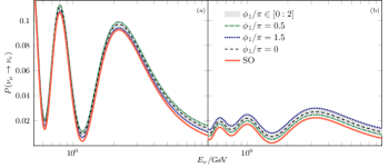
Figure 1: Oscillation probability depending on the neutrino energy for DUNE experiment. The figures ($\mathrm{a}$) and ($\mathrm{b}$) represent the $\nu_{\mu}\rightarrow\nu_{e}$ and $\bar{\nu}_{\mu}\rightarrow\bar{\nu}_{e}$ appearance channels respectively. The off-diagonal decoherence parameter is $\Gamma_{28}=-\Gamma/\sqrt{3}$. We consider $\Gamma_{28}=-\Gamma/\sqrt{3}$, $\delta_{\mathrm{CP}}/\pi=1.4$, and $\Gamma=2.5\times 10^{-24}\mathrm{GeV}$.

$$\begin{split}&P^{\text{SO}\bigoplus\text{DE}}_{\nu_{\mu}\rightarrow\nu_{e}}=\frac{\big{(}1-e^{-\bar{\Gamma}}\big{)}}{3}+P_{\nu_{\mu}\rightarrow\nu_{e}}^{\text{SO}}e^{-\bar{\Gamma}}-\frac{\bar{\Gamma}_{28}}{\sqrt{3}}\sin{2{\theta_{12}}}\sin^{2}{\theta_{23}}\\ &\times\sin{\phi_{1}}e^{-\bar{\Gamma}}+\bar{\Gamma}_{28}\theta_{13}\frac{\sin{2\theta_{23}}}{2\sqrt{3}(A-1)A\Delta}\bigg{(}\big{(}(1-A^{2})\cos{\delta}\\ &+A^{2}\cos{(\delta-\Delta)}-\cos{(\delta-A\Delta)}\big{)}\cos{\phi_{1}}+\big{(}(1-A^{2})\sin{\delta}\\ &+A^{2}\sin{(\delta-\Delta)}-\sin{(\delta-A\Delta)}\big{)}\cos{2\theta_{12}}\sin{\phi_{1}}\bigg{)}e^{-\bar{\Gamma}}\\ &+\bar{\Gamma}_{28}\alpha_{\Delta}\frac{\sin{2{\theta_{12}}}}{\sqrt{3}A^{2}\Delta}\bigg{(}2\sin^{2}{\bigg{(}\frac{A\Delta}{2}\bigg{)}}\cos{2\theta_{23}}\cos{\phi_{1}}-\cos{2\theta_{12}}\\ &\times\sin^{2}{\theta_{23}}\big{(}\sin{A\Delta}-A\Delta\big{)}\sin{\phi_{1}}\bigg{)}e^{-\bar{\Gamma}}+...\\ \end{split}$$ (11)

where $P_{\nu_{\mu}\rightarrow\nu_{e}}^{\text{SO}}$ is the SO probability in matter ($t\rightarrow L$), $\Delta=(m^{2}_{3}-m^{2}_{1})L/(2E)$ and $A=\sqrt{2}G_{F}n_{e}L/\Delta$, where $G_{F}$ is the Fermi constant, $n_{e}$ is the electron number density and $L$ is the source-detector distance. The validity of the transition probability formula relies on having the parameter-perturbative expansion $\bar{\Gamma}_{28}$, $\bar{\Gamma}_{28}\theta_{13}$ and $\bar{\Gamma}_{28}\alpha_{\Delta}$ of order: $10^{-2}$, $10^{-3}$, and $10^{-4}$, respectively. For instance, the latter values can be attained for $|\Gamma_{28}|=2\times 10^{-24}$ GeV, and at DUNE baseline $L=1300$ km. Furthermore, to get the antineutrino transition probability is enough to: $\phi_{1}\rightarrow-\phi_{1}$, $\delta\rightarrow-\delta$ and $A\rightarrow-A$, meanwhile, the $\nu_{\mu}$ survival probability formula is not shown due to its negligible decoherence effect.

The $\nu_{\mu}\rightarrow\nu_{e}$ transition probability displayed in Fig. 1 is numerically calculated at DUNE baseline and for the maximum value of $\Gamma_{28}=-\Gamma/\sqrt{3}$, with $\Gamma=2.5\times 10^{-24}$ GeV and the following values for the SO parameters, taken from Nufit : $\theta_{12}=33.82^{\circ}$, $\theta_{13}=8.61^{\circ}$, $\theta_{23}=48.3^{\circ}$, $\Delta m_{21}^{2}=7.39\times 10^{-5}\mathrm{eV}^{2}$, and $\Delta m_{31}^{2}=2.523\times 10^{-3}\mathrm{eV}^{2}$ (normal hierarchy), that are going to be fixed along this letter. The Dirac CP phase is taken as: $\delta_{\mathrm{CP}}^{true}/\pi=1.4$ inspired in the hint given by the T2K experiment Abe:2019vii From this figure it is notorious the energy-independent increase of the $\text{SO}\bigoplus\text{DE}$ probability respect to standard one, regardless the value of $\phi_{1}$, a feature that has been already pointed out in Carpio:2017nui ; Carpio:2018gum , for other shape of the decoherence matrix. However, the intensity of this increment depends on $\phi_{1}$, for example, in case of $\phi_{1}/\pi=1.5$ ($\phi_{1}/\pi=0.5$) the $\text{SO}\bigoplus\text{DE}$ neutrino (antineutrino) probability grows much less than its antineutrino (neutrino) counterpart. For $\phi_{1}/\pi=0$ the gain is proportionally the same for both, neutrinos or antineutrinos.

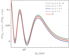
Figure 2: CP asymmetry depending on the neutrino energy. The off-diagonal decoherence parameter is $\Gamma_{28}=-\Gamma/\sqrt{3}$. We consider $\delta_{\mathrm{CP}}/\pi=1.4$, and $\Gamma=2.5\times 10^{-24}\mathrm{GeV}$.

In order to quantify the CP violating effects from the extra terms containing the Majorana phase given in our perturbatives formulae, we use the CP violation asymmetry $\Delta P=P_{\nu_{\mu}\rightarrow\nu_{e}}-P_{\bar{\nu}_{\mu}\rightarrow\bar{\nu}_{e}}$:

$$\Delta P^{\text{SO}\bigoplus\text{DE}}\simeq\Delta P^{\text{SO}}e^{-\bar{\Gamma}}+\frac{2\bar{\Gamma}}{3}\sin{2{\theta_{12}}}\sin^{2}{\theta_{23}}\sin{\phi_{1}}e^{-\bar{\Gamma}}+...$$ (12)

here it is displayed only the leading term $\bar{\Gamma}_{28}\sim\cal{O}$ (0.01) taken $\Gamma_{28}=-\Gamma/\sqrt{3}$, which is its maximum allowed value. The predictions from Eq. (12) are illustrated in Fig. 2 where the $\nu_{\mu}\rightarrow\nu_{e}(\bar{\nu}_{\mu}\rightarrow\bar{\nu}_{e})$ transition probability is numerically calculated at DUNE baseline for $\Gamma_{28}=-\Gamma/\sqrt{3}$, with $\Gamma=2.5\times 10^{-24}$ GeV. In Fig. 2 we see how the overall negative (positive) sign of the decoherence contribution for $\phi_{1}/\pi=1.5$ ($\phi_{1}/\pi=0.5$) diminish (increases) the $\Delta P$ amplitude, whilst for $\phi_{1}/\pi=0.0$ is, as expected, nearly equal to the SO case.

IV Simulation and Results

The DUNE and T2HK simulated data samples are generated with GLoBES Huber:2004ka ; Huber:2007ji and nuSQuIDS Delgado:2014kpa introducing the configuration and inputs from Alion:2016uaj ; Abe:2018uyc ; Acciarri:2015uup ; Huber:2007em , and selecting the optimized fluxes for neutrino and antineutrino with $5$ years of exposure time per each mode for DUNE with a 40-kt detector. While for T2HK, with 258-kt detector, we consider $3$ and $9$ years for neutrino and antineutrino mode, respectively. These simulated samples are created for non-null values of $\Gamma^{true}$ and $\phi_{1}^{true}$ and for a value of the Dirac CP violation phase set on the measurement performed by the T2K experiment: $\delta_{\mathrm{CP}}^{true}/\pi=1.4$ Abe:2019vii . At this point it is important to mention that due to the small statistics and the large size of the uncertainties, we disregard the measurement of the Dirac CP violation claimed by NOvA experiment, which is $\delta_{\mathrm{CP}}/\pi\sim 0.82$ novaresults . In this analysis, the T2K measurement is considered as the true value of the Dirac CP violation phase since it should be unaltered by any quantum decoherence effects. This is because of the small size of the higher decoherence contributions that would be $\bar{\Gamma}\sim\cal{O}\text{(0.001)}$, a consequence of combining the source-detector distance of the T2K experiment with the $\Gamma$ elected for this study. It should be expected, that the T2HK experiment, with the same source-detector distance, would be also unaffected by the quantum decoherence effects. Within our analysis, the T2HK Dirac CP violation phase simulated measurement, which is an upgrade in the precision of the one performed at T2K, will be used as a reference point with the expectations at DUNE. The $\chi^{2}$ analysis for DUNE and T2HK relies on the comparison between the SO phenomena, adopted as theoretical hypothesis, and simulated data that incorporates the quantum decoherence effects, where the prescription given in Carpio:2018gum ; Diaz:2020aax is followed. The calculation of the $\Delta\chi^{2}$ is described by:

$$\small\begin{split}\Delta\chi^{2}=&\chi^{2}(\theta_{13}^{test},\delta_{\mathrm{CP}}^{test};\theta_{13}^{true},\delta_{\mathrm{CP}}^{true},\Gamma^{true},\phi_{1}^{true})\\ &-\chi_{min}^{2}(\theta_{13}^{fit},\delta_{\mathrm{CP}}^{fit};\theta_{13}^{true},\delta_{\mathrm{CP}}^{true},\Gamma^{true},\phi_{1}^{true})\end{split}$$ (13)

where $\theta_{13}^{fit}$ and $\delta_{\mathrm{CP}}^{fit}$ are the best-fit points which minimizes the $\chi^{2}$, considering priors at $3\sigma$ for the rest of the oscillation parameters but $\delta_{\mathrm{CP}}$. The DUNE and T2HK $\Delta\chi^{2}$ contours, projected into $\sin^{2}{\theta_{13}}$ vs $\delta_{\mathrm{CP}}$ planes and obtained after marginalizing over the rest of SO parameters, are presented in Fig. 3. As expected, for T2HK, the $\sin^{2}{\theta^{fit}_{13}}$ and $\delta^{fit}_{\mathrm{CP}}$ are similar to the true ones being unmodified by the parameters chosen for decoherence. Meanwhile, for DUNE there is a slight increase of $\sin^{2}{\theta^{fit}_{13}}$, respect to the $\sin^{2}{\theta^{true}_{13}}(=0.0224)$, explicitly shown in Table. 1. This increment is the consequence of trying to adjust the theoretical hypothesis, SO, with the energy-independent increase of the $\text{SO}\bigoplus\text{DE}$ probability amplitude embodied in the data, and modulated by the intensity of $\Gamma$ (see the third term of Eq. 11).

Figure 3: $\Delta\chi^{2}$ contours (2 dof) considering the effects of decoherence with Majorana phases on the standard oscillation fits. The solid and dashed lines are decoherence with $\Gamma_{28}=-\Gamma/\sqrt{3}$ for the DUNE and T2HK experiments, respectively. The left column is $\Gamma=2.5\times 10^{-24}\mathrm{GeV}$ and the right column is $\Gamma=3.5\times 10^{-24}\mathrm{GeV}$. We consider $\delta_{\mathrm{CP}}^{true}/\pi=1.4$.

$\Gamma=2.5\times 10^{-24}\ \mathrm{GeV}$	$\phi_{1}/\pi=0.5$	$\phi_{1}/\pi=1.0$	$\phi_{1}/\pi=1.5$
$\sin^{2}\theta_{13}^{fit}$	$0.0241$	$0.0242$	$0.0247$
$N_{\sigma}$	$0.31\sigma$	$0.34\sigma$	$0.55\sigma$
$\delta_{\mathrm{CP}}^{fit}/\pi$	$1.43$	$1.33$	$1.13$
$N_{\sigma}$	$0.08\sigma$	$1.19\sigma$	$4.34\sigma$
$\Gamma=3.5\times 10^{-24}\ \mathrm{GeV}$	$\phi_{1}/\pi=0.5$	$\phi_{1}/\pi=1.0$	$\phi_{1}/\pi=1.5$
$\sin^{2}\theta_{13}^{fit}$	$0.0247$	$0.0250$	$0.0256$
$N_{\sigma}$	$0.54\sigma$	$0.61\sigma$	$0.87\sigma$
$\delta_{\mathrm{CP}}^{fit}/\pi$	$1.44$	$1.28$	$1.06$
$N_{\sigma}$	$0.14\sigma$	$2.37\sigma$	$5.47\sigma$

Table 1: Fitted values for $\sin^{2}\theta_{13}$, $\delta_{\mathrm{CP}}$ and their respective shifts in terms of $\sigma$ units. We consider $\delta_{\mathrm{CP}}^{true}/\pi=1.4$

The $\delta^{fit}_{\mathrm{CP}}$ for DUNE, when $\phi_{1}/\pi=1.5$, is moving away from $\delta_{\mathrm{CP}}^{true}/\pi(=1.4)$ towards $\sim\pi$, minimizing the magnitude of the CP violation asymmetry. For $\phi_{1}/\pi=0.5$ the $\delta^{fit}_{\mathrm{CP}}$ takes almost exactly the value of the true one going in the direction to maximize the CP violation asymmetry. Both features, expressed numerically in Table. 1, can be explained from the need to accommodate the reduction (increase) of $\Delta P$, when $\phi_{1}/\pi=1.5(0.5)$, seen in Fig. 2. The quantified dislocation, in terms of $\sigma$, from $\sin^{2}{\theta^{fit}_{13}}$ and $\delta_{\mathrm{CP}}^{fit}$ (for DUNE) to the corresponding true ones (for T2HK), for $\Gamma=\{2.5,3.5\}\times 10^{-24}\mathrm{GeV}$ and $\phi_{1}/\pi=\{0.0,0.5,1.5\}$, is depicted in Table 1. For $\Gamma=3.5(2.5)\times 10^{-24}\mathrm{GeV}$ the most prominent shift is found for $\phi_{1}/\pi=1.5$ with $0.87(0.55)\sigma$ and $5.47(4.34)\sigma$ for $\sin^{2}{\theta^{fit}_{13}}$ and $\delta_{\mathrm{CP}}^{fit}$, respectively. While, for $\Gamma=3.5\ (2.5)\times 10^{-24}\ \mathrm{GeV}$, the dislocation of $\delta_{\mathrm{CP}}^{fit}$ reaches $3\sigma$ $(2\sigma)$ and $5\sigma$ $(3\sigma)$ when $\phi_{1}/\pi$ takes values below $1.01$ $(1.03)$ and $1.30$ $(1.10)$, respectively, the $\sin^{2}{\theta^{fit}_{13}}$ is clearly stable in front of changes along the $\phi_{1}$ interval. The less significant distortion is for $\phi_{1}/\pi=0.5$ with $0.54(0.31)\sigma$ and $0.14(0.08)\sigma$ for $\sin^{2}{\theta^{fit}_{13}}$ and $\delta_{\mathrm{CP}}^{fit}$, respectively. A way to discriminate between different values of $\phi_{1}$ is through the ratio ($\cal R$) of the number of $\sigma$ deviation for $\sin^{2}{\theta^{fit}_{13}}$ to the corresponding ones for $\delta_{\mathrm{CP}}^{fit}$. In fact, a sort of discernment is achieved, for instance, for $\Gamma=3.5(2.5)\times 10^{-24}\ \mathrm{GeV}$, ${\cal R}\sim 0.16(0.13)-0.26(0.29)$ for the interval $\phi_{1}/\pi=1.0,1.5$ reaching values up to $\sim 3.86(3.88)$ for $\phi_{1}/\pi=0.5$. A plus that reinforce the utility of $\cal R$ it is its low variations against changes of $\Gamma$.

The aforementioned analysis had the purpose of searching for distortions in $\sin^{2}{\theta^{fit}_{13}}$ and $\delta_{\mathrm{CP}}^{fit}$, considering pure SO as theoretical hypothesis. Now, the aim is to go one step further and to explore the capacity of DUNE for measuring the Majorana phase, and also $\Gamma$, under the (SO) plus decoherence (DE) as theoretical hypothesis, for $\phi_{1}/\pi=0.5,1,1.5$ and for $\Gamma=4.5,5.5\times 10^{-24}\ \mathrm{GeV}$. The latter values cannot be compared with the limits imposed by Ice Cube Coloma:2018idr since we are considering a non-diagonal scenario for the decoherence matrix. In Fig. 4 the different allowed regions are displayed considering 68 $\%$ and 90 $\%$ C.L for 2 dof. Here it is seen that DUNE is able to measure $\phi_{1}/\pi=1.50\pm 0.35(0.32)$ and $\phi_{1}/\pi=0.50\pm 0.35(0.32)$ and $\Gamma=4.50\pm 1.38(5.50\pm 1.42)\times 10^{-24}\ \mathrm{GeV}$. While for $\phi_{1}/\pi=1.0\pm 0.19(0.15)$ a $\Gamma=4.50\pm 1.42(5.50\pm 1.46)\times 10^{-24}\ \mathrm{GeV}$ is obtained. It is interesting to remark that either for $\phi_{1}/\pi=0.5$ or $1.5$ the value of $\pi$ is excluded at $90\%$ C.L., independent the value of $\Gamma$. Thus, we are able to separate between these different values of $\phi_{1}$.

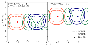
Figure 4: DUNE’s ability to constrain (2 dof) the decoherence parameter and the Majorana phase. The red, green and blue lines represent $\phi^{true}/\pi=0.5,1.0,1.5$, respectively.

V Summary and Conclusions

We demonstrated the possibility of uncovering the Majorana nature of neutrinos in the DUNE experiment if a decoherence environment, with some determined characteristics, interacts with the neutrino system. Planck scale physics could be causing this decoherence environment. Our approach is at first to show the strong displacement that it would be exhibited by the measured value of $\delta_{\mathrm{CP}}$ at DUNE, in comparison with the one measured at T2HK, which would be unaffected by the decoherence effects. This displacement can be as large as 5.47 $\sigma$ for a Majorana phase $\phi_{1}/\pi=1.5$ and a decoherence parameter $\Gamma=3.5\times 10^{-24}\ \mathrm{GeV}$. At next, we assessed the power of DUNE experiment in constraining the Majorana phase achieving, for instance, a precision of $23\%$ ($21\%$) for $\phi_{1}/\pi=1.5$ with $\Gamma=4.5(5.5)\times 10^{-24}\mathrm{GeV}$. These values of precision are compatible with the current results on the Dirac CP phase reached by the T2K experiment Abe:2019vii . Finally, we can conclude that, if decoherence exists in the manner is predicted here, there would be an interesting chance for DUNE to perform a first time a measurement of the Majorana CP phase, with some reasonable uncertainties.

VI Acknowledgements

A. M. Gago acknowledges funding by the Dirección de Gestión de la Investigación at PUCP, through grants DGI-2017-3-0019 and DGI 2019-3-0044. F. N. Díaz acknowledges CONCYTEC for the graduate fellowship under Grant No. 236-2015-FONDECYT. The authors also want to thank F. de Zela, J. Jones-Pérez, J. L. Bazo, C. A. Argüelles and Mario A. Acero for useful suggestions and reading the manuscript.

Appendix A Analysis of the $\rho^{\alpha}_{j}$ for different parametrizations

The starting point of our analysis are the coefficients $\rho^{\alpha}_{j}$, where $j=0,1,...,8$ and $\alpha=e,\mu,\tau$, which are expressed in terms of the mixing matrix Gago:2002na :

$$\begin{split}\rho_{0}^{\alpha}&=\sqrt{2/3}\\ \rho_{1}^{\alpha}&=2\mathrm{Re}(U^{*}_{\alpha 1}U_{\alpha 2})\\ \rho_{2}^{\alpha}&=-2\mathrm{Im}(U^{*}_{\alpha 1}U_{\alpha 2})\\ \rho_{3}^{\alpha}&=|U_{\alpha 1}|^{2}-|U_{\alpha 2}|^{2}\\ \rho_{4}^{\alpha}&=2\mathrm{Re}(U^{*}_{\alpha 1}U_{\alpha 3})\\ \rho_{5}^{\alpha}&=-2\mathrm{Im}(U^{*}_{\alpha 1}U_{\alpha 3})\\ \rho_{6}^{\alpha}&=2\mathrm{Re}(U^{*}_{\alpha 2}U_{\alpha 3})\\ \rho_{7}^{\alpha}&=-2\mathrm{Im}(U^{*}_{\alpha 2}U_{\alpha 3})\\ \rho_{3}^{\alpha}&=\frac{1}{\sqrt{3}}(|U_{\alpha 1}|^{2}+|U_{\alpha 2}|^{2}-2|U_{\alpha 3}|^{2})\\ \end{split}$$ (14)

where the $U_{\alpha j}$ are the matrix elements of the PMNS matrix ($U_{\mathrm{PMNS}}$) Maki:1962mu without taking into account the Majorana phases.

A.1 Symmetrical Parametrization of the mixing matrix

The elements of symmetric parametrization of the mixing matrix, given in Eq. (5) in Rodejohann:2011vc , assuming the relation $\delta=\phi_{13}-\phi_{12}-\phi_{23}$, can be written as follows:

$$\begin{split}U_{e1}&\rightarrow U_{e1}\\ U_{e2}&\rightarrow U_{e2}e^{-i\phi_{12}}\\ U_{e3}&\rightarrow U_{e3}e^{-i(\phi_{23}+\phi_{12})}\\ U_{\mu 1}&\rightarrow U_{\mu 1}e^{i\phi_{12}}\\ U_{\mu 2}&\rightarrow U_{\mu 2}\\ U_{\mu 3}&\rightarrow U_{\mu 3}e^{-i\phi_{23}}\\ U_{\tau 1}&\rightarrow U_{\tau 1}e^{i(\phi_{23}+\phi_{12})}\\ U_{\tau 2}&\rightarrow U_{\tau 2}e^{i\phi_{23}}\\ U_{\tau 3}&\rightarrow U_{\tau 3}\\ \end{split}$$ (15)

where $\phi_{13}$, $\phi_{12}$ and $\phi_{23}$ are the CP phases used in Rodejohann:2011vc .

The corresponding ${\rho}_{j}^{\alpha}$ are described by the following relations:

$$\begin{split}{\rho}_{1}^{\alpha}&\rightarrow\rho_{1}^{\alpha}\cos{\phi_{12}}-\rho_{2}^{\alpha}\sin{\phi_{12}}\\ {\rho}_{2}^{\alpha}&=\rho_{2}^{\alpha}\cos{\phi_{12}}+\rho_{1}^{\alpha}\sin{\phi_{12}}\\ {\rho}_{3}^{\alpha}&\rightarrow\rho^{\alpha}_{3}\\ {\rho}_{4}^{\alpha}&\rightarrow\rho_{4}^{\alpha}\cos{(\phi_{12}+\phi_{23})}-\rho_{5}^{\alpha}\sin{(\phi_{12}+\phi_{23})}\\ {\rho}_{5}^{\alpha}&\rightarrow\rho_{5}^{\alpha}\cos{(\phi_{12}+\phi_{23})}+\rho_{4}^{\alpha}\sin{(\phi_{12}+\phi_{23})}\\ {\rho}_{6}^{\alpha}&\rightarrow\rho_{6}^{\alpha}\cos{\phi_{23}}-\rho_{7}^{\alpha}\sin{\phi_{23}}\\ {\rho}_{7}^{\alpha}&\rightarrow\rho_{7}^{\alpha}\cos{\phi_{23}}+\rho_{7}^{\alpha}\sin{\phi_{23}}\\ {\rho}_{8}^{\alpha}&\rightarrow\rho^{\alpha}_{8},\end{split}$$ (16)

where ${\rho}_{j}^{\alpha}$ are given in Eq. (14)

A.2 Particle data group parametrization type I: PDG I

Here we analyze the mixing matrix parametrization given in Tanabashi:2018oca , which includes the Majorana phases $\phi_{1}$ and $\phi_{2}$:

$$U_{\text{Majorana}}=U_{\text{PMNS}}.\text{diag}(\exp{i\phi_{1}},\exp{i\phi_{2}},1)$$ (17)

The corresponding ${\rho}_{j}^{\alpha}$ are described by the following equations:

$$\begin{split}{\rho}_{1}^{\alpha}&\rightarrow\rho_{1}^{\alpha}\cos{\Delta\phi}+\rho_{2}^{\alpha}\sin{\Delta\phi}\\ {\rho}_{2}^{\alpha}&\rightarrow\rho_{2}^{\alpha}\cos{\Delta\phi}-\rho_{1}^{\alpha}\sin{\Delta\phi}\\ {\rho}_{3}^{\alpha}&\rightarrow\rho^{\alpha}_{3}\\ {\rho}_{4}^{\alpha}&\rightarrow\rho_{4}^{\alpha}\cos{\phi_{1}}-\rho_{5}^{\alpha}\sin{\phi_{1}}\\ {\rho}_{5}^{\alpha}&\rightarrow\rho_{5}^{\alpha}\cos{\phi_{1}}+\rho_{4}^{\alpha}\sin{\phi_{1}}\\ {\rho}_{6}^{\alpha}&\rightarrow\rho_{6}^{\alpha}\cos{\phi_{2}}-\rho_{7}^{\alpha}\sin{\phi_{2}}\\ {\rho}_{7}^{\alpha}&\rightarrow\rho_{7}^{\alpha}\cos{\phi_{2}}+\rho_{6}^{\alpha}\sin{\phi_{2}}\\ {\rho}_{8}^{\alpha}&\rightarrow\rho^{\alpha}_{8},\end{split}$$ (18)

Below, we present in table 2 a summary of the equivalences between the different parameterizations.

Sym. $\leftrightarrow$ PDG I	Sym. $\leftrightarrow$ Our Work	PDG I $\leftrightarrow$ Our Work
$\phi_{12}+\phi_{23}\leftrightarrow\phi_{1}$	$\ \ \ \ \ \ \ \ \phi_{12}\leftrightarrow\phi_{1}$	$\ \hskip 0.56917pt\phi_{1}\leftrightarrow\Delta\phi$
$\ \ \ \ \ \ \ \ \phi_{23}\leftrightarrow\phi_{2}$	$\phi_{12}+\phi_{23}\leftrightarrow\phi_{2}$	$\phi_{2}\leftrightarrow\phi_{1}$
$\ \ \ \ \ \ \ \ \ \phi_{12}\leftrightarrow\Delta\phi$	$\ \ \ \ \ \ \ \ \ \ \ \ \phi_{23}\leftrightarrow-\Delta\phi$	$\ \hskip 0.56917pt\Delta\phi\leftrightarrow-\phi_{2}$

Table 2: Parameterizations comparison.

where $\Delta\phi=\phi_{1}-\phi_{2}$.

Appendix B Probability Calculation

For solving ${\varrho^{\prime}}_{m}^{\alpha}(t)$ we must start with the next differential equation:

$$\dot{{\varrho^{\prime}}_{m}^{\alpha}}=({\bf H_{m}+D}_{m}^{nd}){\varrho^{\prime}}_{m}^{\alpha},$$ (19)

which is similar to Eq.(2) presented in our letter. Before continue, we must point out that the following procedure is similar to the one given in Carpio:2017nui . The Eq.(19) can be simplified using this change of variable:

$${\varrho}_{m}^{\alpha}(t)=e^{{\bf H_{m}}t}{\tilde{\varrho}}^{\alpha}(t),$$ (20)

then the Eq. 19 :

$$e^{{\bf H_{m}}t}\dot{\tilde{\varrho}}^{\alpha}+{\bf H}_{m}e^{{\bf H_{m}}t}\tilde{\varrho}^{\alpha}={\bf(H_{m}+D_{m}^{nd})}e^{{\bf H_{m}}t}{\tilde{\varrho}}^{\alpha}$$ (21)

thus we get:

$$\dot{\tilde{\varrho}}^{\alpha}=e^{-{\bf H_{m}}t}{\bf D_{m}^{nd}}e^{-{\bf H_{m}}t}\tilde{\varrho}^{\alpha},$$ (22)

the matrix $e^{-{\bf H_{m}}t}{\bf D_{m}^{nd}}e^{-{\bf H_{m}}t}$ can be expanded perturbatively in power series of the small parameters $\theta_{13}$, and $\alpha_{\Delta}$ which turns out to be:

$$e^{-{\bf H_{m}}t}{\bf D_{m}^{nd}}e^{-{\bf H_{m}}t}=\Gamma_{ij}(\tilde{D}^{(0)}+\theta_{13}\tilde{D}^{(\theta_{13})}+\alpha_{\Delta}\tilde{D}^{(\alpha_{\Delta})}+...)$$ (23)

we can factor out the decoherence parameter $\Gamma_{ij}$ since it is a common factor of all the elements in the decoherence matrix $\bf D_{m}^{nd}$ in the MMB (a consequence of its definition in the mass vacuum basis that is an off-diagonal matrix with only non-null terms in a given $-\Gamma_{ij}$ element). Replacing Eq.(23) into Eq.(22):

$$\dot{\tilde{\varrho}}^{\alpha}=\Gamma_{ij}(\tilde{D}^{(0)}+\theta_{13}\tilde{D}^{(\theta_{13})}+\alpha_{\Delta}\tilde{D}^{(\alpha_{\Delta})}+...)\tilde{\varrho}^{\alpha}$$ (24)

the above equation can be solved perturbatively treating $\tilde{\varrho}^{\alpha}$ as a power series in $\theta_{13}$, $\alpha_{\Delta}$ and $\Gamma_{ij}$:

$$\begin{split}\tilde{\varrho}^{\alpha}&=\tilde{\varrho}^{(0)}+\theta_{13}\tilde{\varrho}^{(\theta)}+\alpha_{\Delta}\tilde{\varrho}^{(\alpha_{\Delta})}+\alpha_{\Delta}\theta_{13}\tilde{\varrho}^{(\alpha_{\Delta}\theta_{13})}+...\\ &+\Gamma_{ij}\tilde{\varrho}^{(\Gamma_{ij})}+\Gamma_{ij}\theta_{13}\tilde{\varrho}^{(\Gamma_{ij}\theta_{13})}+\Gamma_{ij}\alpha_{\Delta}\tilde{\varrho}^{(\Gamma_{ij}\alpha_{\Delta})}+...\end{split}$$ (25)

Then substituing Eq.(25) into Eq.(24) we produce a sequence of first order differential equations each of them collecting equal power terms. The $\Gamma_{ij}$-independent terms of the $\tilde{\varrho}^{\alpha}$ expansion: $\tilde{\varrho}^{(0)}+\theta_{13}\tilde{\varrho}^{(\theta)}+\alpha_{\Delta}\tilde{\varrho}^{(\alpha_{\Delta})}+\alpha_{\Delta}\theta_{13}\tilde{\varrho}^{(\alpha_{\Delta}\theta_{13})}+...\$ corresponds to the initial condition $\tilde{\varrho}^{\alpha}(0)$, which is constant in time and coincides with the initial condition for the standard oscillation case, since at that instant the environment is decoupled (not interacting) with the neutrino system. Considering all the later plus the condition that ${\varrho^{\prime}}^{\alpha}_{m}(0)=\tilde{\varrho}^{\alpha}(0)$, we can rewrite Eq.(20) as follows:

$${\varrho^{\prime}}_{m}^{\alpha}(t)=e^{{\bf H_{m}}t}({\varrho^{\prime}}_{m}^{\alpha}(0)+\bar{\Gamma}_{ij}(...)).,$$ (26)

with $\bar{\Gamma}_{ij}=\Gamma_{ij}t$. The second term at the right-hand side of the equation above contains the explicit solution of the power series of ${\varrho}^{\alpha}$.

Appendix C CP-odd, CPT-odd terms and Majorana phases

$\mathrm{CPV}$	$\mathrm{CPTV}$	Non-null Majorana phase
$\Gamma_{13},\Gamma_{23},\Gamma_{18},\Gamma_{28},\Gamma_{12}$	$\Gamma_{23},\Gamma_{28},\Gamma_{12}$	$\phi_{1}$
$\Gamma_{34},\Gamma_{35},\Gamma_{48},\Gamma_{58},\Gamma_{45}$	$\Gamma_{35},\Gamma_{58},\Gamma_{45}$	$\phi_{2}$
$\Gamma_{37},\Gamma_{36},\Gamma_{68},\Gamma_{67},\Gamma_{78}$	$\Gamma_{37},\Gamma_{67},\Gamma_{78}$	$\Delta\phi$
$\Gamma_{14},\Gamma_{24},\Gamma_{15},\Gamma_{25}$	$\Gamma_{24},\Gamma_{15}$	$\phi_{1},\phi_{2}$
$\Gamma_{16},\Gamma_{17},\Gamma_{26},\Gamma_{27}$	$\Gamma_{17},\Gamma_{26}$	$\phi_{1},\Delta\phi$
$\Gamma_{46},\Gamma_{47},\Gamma_{56},\Gamma_{57}$	$\Gamma_{47},\Gamma_{56}$	$\phi_{2},\Delta\phi$

Table 3: Violation of symmetries by non-diagonal decoherence elements and their dependence on the Majorana phases.

In table 3 we present a classification of the correspondence between each one of the off-diagonal elements $\Gamma_{ij}$ and $\phi_{1}$, $\phi_{2}$, or $\Delta\phi$, also pointing out its connection with CP-odd, CPT-odd terms or both in the oscillation probabilities which incorporates quantum decoherence.