Transmission in a Fano-Anderson chain with a topological defect

Abstract

The Fano-Anderson chain consists of a linear lattice with a discrete side-unit, and exhibits Fano-resonant scattering due to coupling between the discrete states of the side-unit with the tight-binding continuum. We study Fano-resonance-assisted transport for the case of a topologically non-trivial side unit. We find that the topology of the side unit influences the transmission characteristics which thus can be an effective detection tool of the topological phases of the side unit. Furthermore, we explore the role of dual links between the linear tight binding chain and the side unit. The secondary connection between the main chain and the side unit can modify the position or width of the Fano resonance dip in the transmission probability, and thus yield additional control.

I Introduction

Fano resonance [1, 2] is a quantum phenomenon arising from the interaction between a continuum band of states and discrete states, that has been explored in a wide variety of settings ranging from nuclear, atomic, molecular and condensed matter systems [3, 4], to electronics [5, 6] and optics [7, 8, 9]. Linear wave equations on Hamiltonian lattices can also give rise to Fano resonances if local defects are present [3, 10]. The Fano-Anderson chain made up of a linear chain interacting with a single defect site is the simplest example for such a system [11]. The discrete state introduced by the defect allows additional propagation paths for scattering waves which interfere constructively or destructively. This discrete-state-assisted interference may lead to perfect transmission or perfect reflection along with an asymmetric resonance profile.

Recent years have seen quickly growing interest in the exploration of Fano resonance associated with many different kinds of modified Fano-Anderson chains. Examples include systems with a single defect site [12, 13], a linear chain [14], and a Fibonacci chain [15]. One common observation in all these structures is that the Fano resonance profile in the transmission probability shows a dip at the eigen-energies of the side unit interacting with the main chain. Since topological systems [16, 17] are naturally endowed with isolated energy states, one expects interesting Fano scattering properties. Nonetheless, Fano resonances in such topological models have only very recently drawn the first attention [18].

We take the Su-Schieffer-Heeger (SSH) chain as an example for the topological side unit and demonstrate how the Fano transmission profile is affected by the topological-to-trivial phase transition. In the trivial phase, a perfect transmission is observed at energies close to $E=0$. The isolated edge state in the topological phase induces a Fano resonance and leads to a dip in the transmission profile at the energy of the edge state. The trivial to topological transition can be identified from the dip emerging in the transmission profile. A second connection to the side unit enhances the width of the resonance dip, which may be an advantage in real detection systems. The boundary conditions of the SSH chain modify the edge states and the transmission profile is also altered accordingly. This concept can be further extended to two or three dimensional topological systems.

In this article, we employ the transfer matrix method (TMM) to study the transmission profile [19, 11] of the Fano-Anderson chain, which allows for exact analytical expressions describing the transmission characteristics. The method has been used in the past, to explore the Fano-Anderson chain with one connection to the side unit [3]. We focus on a linear chain with two connections to a topological side unit. We derive the exact expression for the transmission coefficient and obtain the conditions for perfect reflection. Our methods are general enough to be applicable to any kind of finite sized side unit, which may be quasi one-dimensional, two-dimensional, or even three-dimensional.

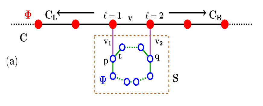
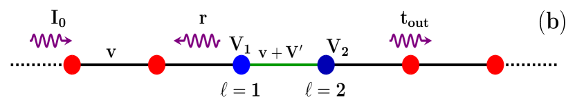
Figure 1: (a) Schematic of the setup with two adjacent connections between the main chain (C) and the $p^{th}$ and $q^{th}$ sites of the side unit (S). These connections have hopping strengths $v_{1}$ and $v_{2}$. The hopping amplitude in the main chain is set to $v$ with onsite wavefunction $\Phi$ and hopping in the side unit $t$. We mark the left and right parts of the main chain as $C_{L}$ and $C_{R}$ and side-unit as $S$ for clarity. (b) Schematic representation of Fano-Anderson chain with effective potentials $V_{1}$ and $V_{2}$ at sites $\ell=1$ and $\ell=2$, respectively, which result after elimination of the side-unit. The effective hopping between these two sites becomes $v+V^{\prime}$.

The manuscript is arranged as follows. In the next section we describe the Fano-Anderson model which is linked to a side unit with two adjacent connections. This section also describes how the transfer matrix method can be used to obtain the conditions needed for Fano resonance. In section III, we present the topological properties of the SSH model considering all possible structures. Further, in section IV, we study Fano resonance in different cases of the SSH model taken as the side unit. Finally, we collect and summarize our findings in the conclusion section.

II Model

We consider a linear tight binding chain connected to a Fano defect chain with two connections between them as shown in Fig. 1. The Hamiltonian for this system is

$$H=H_{c}+H_{s}+H_{cs},$$ (1)

where $H_{c}$ is the Hamiltonian corresponding to the linear chain $C$,

$$H_{c}=v\sum_{\ell}(\Phi^{*}_{\ell+1}\Phi_{\ell}+\Phi^{*}_{\ell}\Phi_{\ell+1}).$$ (2)

Here, $\Phi_{\ell}$ is the complex wave amplitude at the site $\ell$ and $v$ is the coupling strength. $H_{s}$ corresponds to the Hamiltonian for the side chain $S$ with $N$ sites and reads

$$H_{s}=\sum_{i,j=1}^{N}h_{i,j}\Psi^{*}_{i}\Psi_{j},$$ (3)

where $\Psi_{i}$ is the complex wave amplitude at the site $i$ on the side chain and $h_{ij}$ is the coupling strength connecting the sites labeled $i,j$. The third term in the Hamiltonian $H_{cs}$ corresponds to the coupling between the main chain and the side chain, and is given by:

$$H_{cs}=v_{1}\Phi_{1}^{*}\Psi_{p}+v_{2}\Phi_{2}^{*}\Psi_{q}+H.c.,$$ (4)

with $v_{1}$ and $v_{2}$ being the coupling strengths between the main chain and the side chain. Sites $p$ and $q$ are arbitrary and even can be the same. In the absence of the side unit, Bloch’s theorem can be applied to the translationally invariant linear chain $C$ described by Eq. (2). For states $\phi_{\ell}=e^{\iota k\ell}$ one finds energies of propagating waves $E=2v\cos{k}$, where $k$ is the wave number. The side unit acts as a scatterer and introduces extra paths for an incoming wave. This resonant scattering due to the side unit controls the wave propagation in the main chain and we employ the transfer matrix method to obtain the transmission and reflection coefficients associated with the propagation in the main chain $C$ in the presence of a side unit $S$.

The time ($\tau$) dependence from the Schrödinger equation is eliminated using the Ansatz

$$\Phi(\ell,\tau)= A_{\ell}e^{-\iota E\tau},$$ (5)

$$\Psi(j,\tau)= B_{j}e^{-\iota E\tau}.$$ (6)

The time-independent Schrödinger equation corresponding to the Hamiltonian (H) can be written as:

$$EA_{\ell} =v(A_{\ell+1}+A_{\ell-1})+v_{1}B_{p}\delta_{\ell,1}+v_{2}B_{q}\delta_{\ell,2},$$ (7)

$$EB_{i} =\sum_{j=1}^{N}h_{i,j}B_{j}+v_{1}\delta_{i,p}A_{1}+v_{2}\delta_{i,q}A_{2},$$ (8)

where Eq. (7) and Eq. (8) correspond to sites in the main chain and side unit, respectively. To obtain the transmission characteristics in the main chain, the two coupled equations must be solved simultaneously. The complex amplitudes $B_{i}$ in the side unit can be written in terms of the amplitudes $A_{\ell}$ in the main chain as follows. Using Eq. (8), the relation between $B_{i}$ and $A_{\ell}$ can be written as $\mathcal{H}_{N}\mathcal{B}_{N}=\mathcal{A}_{N}$ where $\mathcal{H}_{N}(E)=[EI-H_{s}]_{N\times N}$, $\mathcal{B}_{N}=[B_{1},\ldots,B_{p},\ldots,B_{q},\ldots,B_{N}]^{T}$, $\mathcal{A}_{N}=[0,\ldots,v_{1}A_{1},\ldots,v_{2}A_{2},\ldots,0]^{T}$, with $I$ the identity matrix and $N$ the size of the side chain (S). Inverting the matrix $\mathcal{H}_{N}$ [20], the expressions for $B_{p/q}$ now become

$$B_{p}= v_{1}\alpha_{pp}A_{1}+v_{2}\alpha_{pq}A_{2},$$ (9)

$$B_{q}= v_{1}\alpha_{qp}A_{1}+v_{2}\alpha_{qq}A_{2},$$ (10)

where $\alpha_{ij}(E)=({\mathcal{H}}^{-1}_{N}(E))_{ij}$. The Hermiticity of the Hamiltonian guarantees that $\alpha_{ij}=\alpha^{*}_{ji}$. These equations can be substituted back into Eq. (7) to obtain the wave propagation in the main chain in terms of the amplitudes $A_{l}$ as:

$$EA_{\ell}=(\alpha_{pp}v_{1}^{2}\delta_{\ell,1}+\alpha_{qq}v_{2}^{2}\delta_{\ell,2})A_{\ell}+(v+v_{1}v_{2}\alpha_{pq}\delta_{\ell,1})A_{\ell+1}$$

$$+(v+v_{2}v_{1}\alpha_{qp}\delta_{\ell,2})A_{\ell-1}.$$ (11)

Equation (11) is the modified lattice equation for the main chain incorporating the effects of the scatterer in terms of effective energy dependent potentials $V_{1}(E)=\alpha_{pp}v_{1}^{2}$, $V_{2}(E)=\alpha_{qq}v_{2}^{2}$, and $V^{\prime}(E)=v_{1}v_{2}\alpha_{pq}$ as sketched in Fig. 1b. The energy dependence of the effective potentials allows for resonant scattering and can cause complete transmission or complete reflection of the incoming wave as well as an asymmetric resonance profile. From Fig. 1b, the condition for perfect reflection can be identified as $v=-V^{\prime}(E)$ since the effective hopping between sites $\ell=1$ and $\ell=2$ would then vanish. In the limit $v_{2}\rightarrow 0$ i.e. with just a single connection between the main chain and the side unit, $V_{2}(E)$ and $V^{\prime}(E)$ vanish. Perfect transmission in this case occurs when $|\mathcal{H}_{N-1}|=0\;\text{or}\;V_{1}=\alpha_{pp}=0$ which results in a translationally invariant tight binding chain with no effective scattering and therefore unit transmission. Perfect reflection is instead realized when $|\mathcal{H}_{N}|=0\;\text{or}\;V_{1}=\alpha_{pp}=\infty$ i.e. an infinite onsite potential leads to full reflection or zero transmission [11].

Employing the transfer matrix method (Appendix A) for Eq. (11), the transmission coefficient in terms of the energy of the incoming wave can be written as:

$$T=\frac{v^{2}(4v^{2}-E^{2})|v+V^{\prime}|^{2}}{[\beta v^{2}+\gamma vE-E^{2}M^{{}^{\prime}}_{11}M^{{}^{\prime}}_{22}]},$$ (12)

where $\beta=(M^{{}^{\prime}}_{11}+M^{{}^{\prime}}_{22})^{2}+(M^{{}^{\prime}}_{12}-M^{{}^{\prime}}_{21})^{2}$ and $\gamma=(M^{{}^{\prime}}_{11}-M^{{}^{\prime}}_{22})(M^{{}^{\prime}}_{12}-M^{{}^{\prime}}_{21})$ with $M^{{}^{\prime}}_{11}=[(E-V_{1})(E-V_{2})-|v+V^{\prime}|^{2}]$, $M^{{}^{\prime}}_{12}=-v(E-V_{2})$, $M^{{}^{\prime}}_{21}=v(E-V_{1})$, $M^{{}^{\prime}}_{22}=-v^{2}$. When two side chain sites are simultaneously connected to the main chain, perfect reflection is possible if the energy is tuned in such a way that the condition

$$v+V^{\prime}=0$$ (13)

holds, as can directly be seen in Eq. (12), besides the intuitive way of obtaining it from Fig. 1(b). The condition given in Eq. (13) is a consequence of destructive interference of the different paths available for the wave which results in zero hopping amplitude for transmission across the scattering zone, leading to perfect reflection of the wave.

III SSH chain and topology

In the discussion so far, details of the side unit did not enter. Now we choose the Su-Schieffer-Heeger (SSH) model as the side unit because of its interesting topological properties. The SSH model consists of a network of sites with alternating hopping amplitudes with the Hamiltonian given by

$$H_{s}^{SSH}=\displaystyle\sum_{i=1}^{L}(t\Psi^{*}_{i}\chi_{i}+t^{\prime}\chi^{*}_{i}\Psi_{i+1})+H.c.$$ (14)

where, $\Psi_{i}$, $\chi_{i}$ are the particle wavefunctions on two adjacent sites of the $i^{th}$ unit cell. For the case of our side unit this is sketched in the dotted box of Fig. 2.

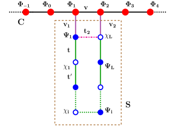
Figure 2: Representation of the site amplitudes of wavefunctions, with the side unit described by a SSH model with inter-cell hopping $t^{\prime}$ and intra-cell hopping $t$. The main chain (C) hopping, and the two connection hoppings are set to $v$, $v_{1}$, and $v_{2}$ respectively. The presence (absence) of the extra hopping $t_{2}=t^{\prime}$ with dashdotted magenta line turns the side unit into a closed (open) chain.

The intra-cell coupling is labeled as $t$ whereas inter-cell coupling is $t^{\prime}$.

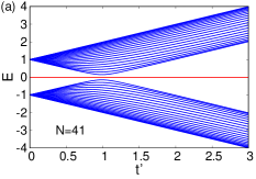
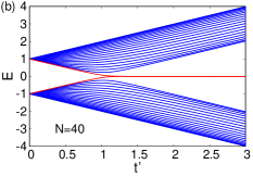
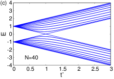
Figure 3: The energy spectrum for the isolated SSH model with different inter-cell hopping $t^{\prime}$ and a constant intra-cell hopping $t=1.0$ with red lines showing the energy of edge states. We show the spectrum for (a) $N=2L\pm 1=41$ sites and (b) $N=2L=40$ sites with open boundary conditions and (c) $N=2L=40$ sites with periodic boundary conditions.

The SSH model is known for its topological features. The winding number changes from zero to one as the system is tuned from $t^{\prime}<t$ to $t^{\prime}>t$, indicating a phase transition from the topological phase to a trivial phase. The dispersion spectrum of the SSH model for different total number of sites $N=2L\pm 1\;\text{or}\;2L$ is depicted in Fig. 3. A chain with an odd number of sites is incompatible with periodic boundary conditions. On the other hand an open chain may have an odd or even number of sites and always gives rise to an edge state with energy $E\approx 0$ in the topological phase. The number of zero energy edge states residing on the ends of the chain depends on the way the chain is terminated at the boundaries.

For odd number of sites ( Fig. 3a), there is always an edge state in the system. When $t^{\prime}<t$ the edge state lies at the end with the hopping $t^{\prime}$ whereas for $t^{\prime}>t$ the edge state lies at the end with the hopping $t$ of the SSH chain. The ratio of the intra-cell to the inter-cell hopping ($\frac{t}{t^{\prime}}$) of the SSH chain controls the position of this edge state. In contrast, for even number of sites, edge states at both ends appear only when $t^{\prime}>t$. The edge states present in the SSH model reside on the ends of the chain and decay in the bulk depending on the ratio of the inter-cell and intra-cell hopping ($\xi\propto\frac{t^{\prime}+t}{t^{\prime}-t}$). The system size should be greater than the decay length for the properties of the edge states to be observable.

IV Fano resonance: SSH chain as the side unit

After a review of the physics of the isolated SSH model, we now explore how coupling it to the main chain affects transport properties on that chain. Here, we take the side unit to be the SSH chain as shown in Fig. 2. The expression for $\Gamma_{N}=|\mathcal{H}_{N}(E)|=|E\mathcal{I}-H_{s}|$ is thus given by

$$\Gamma_{N}=|E\mathcal{I}-H_{s}|=\begin{vmatrix}E&-t&0&0&\ldots&-t_{2}\\ -t&E&-t^{\prime}&0&\ldots&0\\ 0&-t^{\prime}&E&-t&\ldots&\vdots\\ 0&0&\ddots&\ddots&\ddots&-t_{1}\\ -t_{2}&0&0&\ldots&-t_{1}&E\end{vmatrix}_{N\times N}$$ (15)

where $N=2L$ or $2L\pm 1$ is the number of sites in the SSH side unit (with $L$ unit cells on the SSH chain) and $t$, $t^{\prime}$ are two alternate hoppings. Since $t$ and $t^{\prime}$ alternate on the sub-diagonal and super-diagonal of the tridiagonal matrix ($\mathcal{H}_{N}(E)$), one has to write $t_{1}=t$ or $t^{\prime}$ depending on the length $N$, while $t_{2}=0$ for an open chain and $t_{2}=t^{\prime}$ for a closed chain. While the length of the open chain may be odd or even, the closed chain is forced to have an even number of sites, because of geometrical constraints, as we will discuss later. We use $\Gamma_{N-j}^{\{\lambda_{1},\lambda_{2},\ldots,\lambda_{j}\}}$ to represent the determinant of the square matrix with dimension $(N-j)\times(N-j)$ that is formed after the removal of the $\{\lambda_{1},\lambda_{2},\ldots,\lambda_{j}\}^{th}$ rows and columns from the matrix $[E\mathcal{I}-H_{s}]$ given in Eq. (15).

In the following subsections, we separately discuss how the system size of the side-unit and whether the SSH chain is open or closed affects transport in the main chain. The properties of the open and closed SSH chains are quite different due to the presence and absence, respectively, of edge states. The focus of this study is on understanding how the transmission properties carry signatures of these edge-states, which play a crucial role at energies close to zero ($E\sim 0$). Therefore, the first and last site ($n^{th}$) of the SSH chain are connected to the main chain as shown in Fig. 2.

IV.1 Case 1: Open chain with odd N

We now discuss the transport properties of the system when the defect is the open SSH chain with an odd number of sites (Fig. 2). As discussed already, the open chain always possesses one edge state whose location depends on the relative hopping strengths $t,\;t^{\prime}$ as shown in Fig. 3a. When $t^{\prime}<t$, an edge state resides on the last site of the SSH chain and decays in the bulk while in the other limit $t^{\prime}>t$, the edge state resides on the first site. Besides varying the relative strength of $t$ and $t^{\prime}$, we have also considered two different cases for the second connection strength $v_{2}$ i.e. $v_{2}=0$ and $v_{2}\neq 0$. For all scenarios we need to first evaluate the required coefficients of the inverse of the matrix $\mathcal{H}_{N}$. For the particular choice here, we have the relations $\alpha_{11}=\frac{\Gamma_{N-1}^{\{1\}}}{\Gamma_{N}}$, $\alpha_{nn}=\frac{\Gamma_{N-1}^{\{N\}}}{\Gamma_{N}}$, $\alpha_{1n}=\alpha_{n1}=\frac{(tt^{\prime})^{\frac{N-1}{2}}}{\Gamma_{N}}$.

Figure 4: The transmission coefficient $T$ for the open SSH side chain with $N=99$ for a single connection between chain and side unit. We show $T$ as a function of inter-cell hopping $t^{\prime}$ and incoming wave energy $E$. The other parameters are kept constant: $v=1$, $t=1$, $v_{1}=1$ and $v_{2}=0$.

First, we discuss the effect of a single link between the main chain and the side unit i.e. $v_{1}\neq 0;\;v_{2}=0$. For this scenario, perfect reflection ($T=0$) results if $\Gamma_{N}=0$ while perfect transmission ($T=1$) is found for $\Gamma_{N-1}^{\{1\}}=0$. Figure 4 features the transmission coefficient (T) as a function of the incoming energy of the wavefunction (E) and inter-cell hopping $t^{\prime}$. It is observed that for $E=0$, the system shows a clear perfect reflection for $t^{\prime}>t$ with a broad blue region. However, for $t^{\prime}<t$ a thin line is observed within the red region of full transmission as depicted in Fig. 4. The behavior of the transmission coefficient (T) in this case is consistent with the characteristics of the eigenstate of the full Hamiltonian at $E=0$ as shown in Fig. 14 of Appendix B. In the limit $t^{\prime}<t$, the eigenstate at $E=0$ supports no probability amplitude in the main chain and as a consequence, a sharp dip indicating zero transmission is observed as shown in Fig. 4. In the limit $t^{\prime}>t$, for the $E=0$ state, the probability amplitude resides only on one half of the main chain and hence, leads to perfect reflection as indicated by the broad blue region in Fig. 4.

If the second coupling to the Fano defect side chain is added ($v_{2}\neq 0$), the condition for perfect reflection is modified. It is now possible only for those energies that satisfy:

$$v\Gamma_{N}+v_{1}v_{2}(tt^{\prime})^{\frac{N-1}{2}}=0,$$ (16)

where $\Gamma_{N}=\displaystyle\prod_{\theta_{m}}(E\pm\sqrt{t^{2}+{t^{\prime}}^{2}+2tt^{\prime}\cos\theta_{m}})$ with $\theta_{m}=\frac{2\pi m}{N+1}$; $m=1,2,\ldots,\frac{N-1}{2}$ [21].

Figure 5: Transmission as a function of the incoming wave energy $E$ for the couplings between the main chain and the open SSH side chain with $N=99$ for different inter-cell hopping $t^{\prime}$. The system parameters are set to $v_{1}=1$, $v_{2}=1$, $v=1$, $t=1$.

The transmission coefficient as a function of the incoming wave energies and the inter-cell coupling $t^{\prime}$ is shown in Fig. 5. Full reflection is observed at $E=0$ in both the regimes, $t^{\prime}<t$ and $t^{\prime}>t$. In both the cases $t^{\prime}>t$ as well as $t^{\prime}<t$, the zero energy wave propagates to the scattering region of the main chain and reflects back (verified from a study of the full system eigenstates shown in Fig. 15 of the Appendix B). This finally results in minimum transmission through the system. Thus, the narrow line observed for $v_{2}=0$ with $t^{\prime}<t$ in Fig. 4 is modified into a wider blue region when $v_{2}\neq 0$ as shown in Fig. 5.

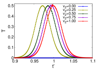
Figure 6: The transmission coefficient as a function of different inter-cell hopping $t^{\prime}$ of the open SSH chain for different second connection strengths $v_{2}$. The other system parameters are kept fixed: $N=99$, $t=v=v_{1}=1$, $E\sim 0$.

We have seen that a connection $v_{2}$ to the side chain significantly modifies the transmission in the system. This motivates us to study how tuning the second coupling strength $v_{2}$ affects transmission for various inter-leg hopping strengths $t^{\prime}$ as shown in Fig. 6. We see that when $v_{2}=0$, for energy close to zero, the transmission is zero for any value of $t^{\prime}$. However, for non-vanishing $v_{2}$ the system shows transmission only in the limit $t^{\prime}\rightarrow t$. As $t^{\prime}$ approaches $t$, the SSH chain starts to behave as a simple nearest-neighbor tight binding chain and for an odd system size it should show perfect reflection for energies $E\sim 0$. But due to the presence of the secondary connection the energy corresponding to perfect reflection (shown in Fig. 18) is given by Eq. (16). Therefore the system shows some transmission for energies close to zero, as shown in Fig. 6. In Appendix C, we discuss the role of the second connection, when the side unit is a simple tight binding linear chain.

IV.2 Case 2: Open chain with even N

Next we explore the SSH open chain with an even number of sites as the side chain. In this case, the isolated SSH model possesses either no edge state (zero energy state) for the case $t^{\prime}<t$ or two edge states located at the two ends for the case $t^{\prime}>t$ as shown in Fig. 3(b).

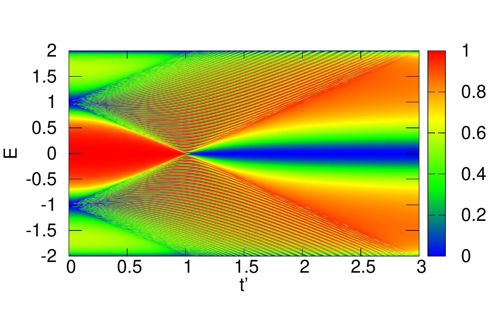
Figure 7: The transmission coefficient (T) for a single coupling between the main chain and an open SSH side chain with $N=100$ as a function of incoming wave energy $E$ and inter-cell hoppings $t^{\prime}$ with other parameters set to $v=1$, $t=1$, $v_{1}=1$, $v_{2}=0$.

In order to understand the transmission in this system, the required coefficients of the inverse matrix $\mathcal{H}_{N}$ are calculated as: $\alpha_{11}=\alpha_{nn}=\frac{\Gamma_{N-1}^{\{1\}}}{\Gamma_{N}}$, $\alpha_{1n}=\alpha_{n1}=\frac{(tt^{\prime})^{\frac{N}{2}}}{t^{\prime}\Gamma_{N}}$. In the single coupling setup to the scatting center ($v_{1}\neq 0;\;v_{2}=0$), the condition for perfect reflection ($T=0$) is again given by $\Gamma_{N}=0$ and the condition for perfect transmission is given by $\Gamma_{N-1}^{\{1\}}=0$. The transmission spectrum as a function of incoming wave energy $E$ and inter-cell hopping $t^{\prime}$ is shown in Fig. 7. At $E\sim 0$, the transmission coefficient undergoes a transition from $1$ (red region) to $0$ (blue region) on switching from the trivial (at $t^{\prime}<t$) to the topological (at $t^{\prime}>t$) phase of the SSH chain as shown in Fig. 7. The propagating wave reflects back from the scattering region in the main chain as depicted by the eigenstate of the full Hamiltonian in Fig. 16 (Appendix B).

The two links to the side chain modify the condition for perfect reflection, which now happens for energies satisfying the equation

$$vt^{\prime}\Gamma_{N}+v_{1}v_{2}(tt^{\prime})^{\frac{N}{2}}=0,$$ (17)

where $\Gamma_{N}=\displaystyle\prod_{\theta_{m}}(E\pm\sqrt{t^{2}+{t^{\prime}}^{2}+2tt^{\prime}\cos\theta_{m}})$. The variable $\theta_{m}$ is calculated numerically using the relation $t\;\Lambda(\theta_{m},\frac{N}{2})+t^{\prime}\;\Lambda(\theta_{m},\frac{N}{2}-1)=0$, where $\Lambda(\theta_{m},l)=\frac{\sin[(l+1)\theta_{m}]}{\sin\theta_{m}}$ [21]. In the case $t^{\prime}<t$, the wave propagates without disturbance in the main chain which results in perfect transmission in the system.

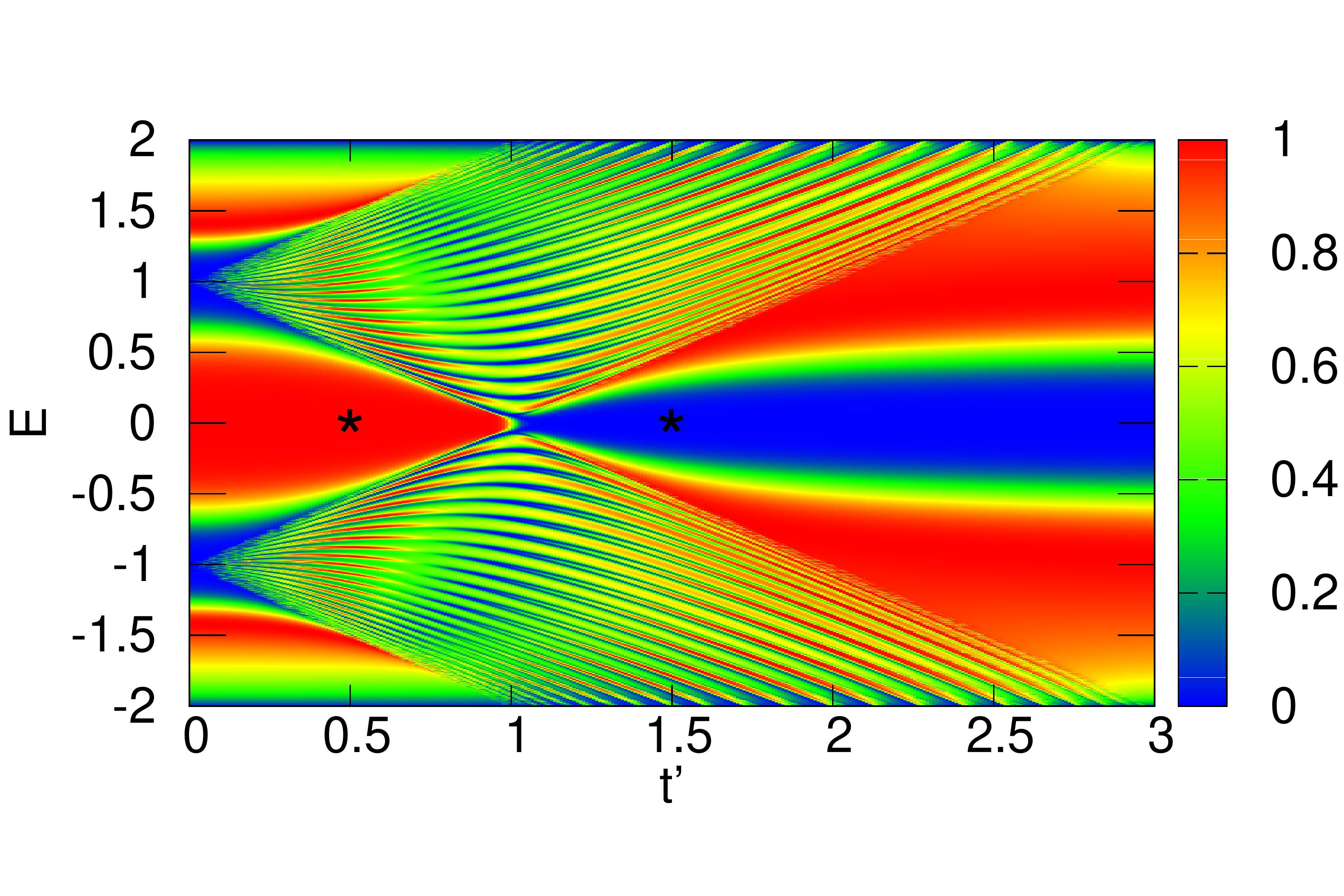
Figure 8: The transmission coefficient $T$ for the open SSH side chain with length $N=100$ for two couplings ($v_{1},\;v_{2}$) between the main chain and the side unit. We show $T$ as a function of inter-cell hopping $t^{\prime}$ and incoming wave energy $E$. The other parameters are kept constant: $v=1$, $t=1$, $v_{1}=1$, $v_{2}=1$. The wave amplitudes corresponding to the two ($*$) symbols are plotted in Fig. 9.

However, in the other limit $t^{\prime}>t$, the main chain is connected to the two edge states of the SSH chain, and therefore, as shown in Fig. 8, minimum transmission is obtained due to the reflection of the incoming wave by these edge states (Fig. 17). Thus, the transmission coefficient $T$ again features a transition from $1$ to $0$ for zero energy when the side chain undergoes a transition from the trivial to the topological phase but the width of the perfect reflection area is increased in the presence of the secondary coupling $v_{2}$. At $E=0$, the transmission coefficient $T$ is unaffected by the secondary connection to the side chain as shown in Fig. 8. This should be seen as a consequence of the robustness of the topologically protected edge states of the SSH chain.

We verify the results by studying the time dependent wave equation

$$i\frac{d}{d\tau}\psi=H\psi$$ (18)

where $H$ is the full Hamiltonian of the system, and $\psi$ is the wavefunction representing wave propagation in the system. The incoming wave is represented by an initial Gaussian wavepacket (time $\tau=0$) localized at a site $l_{0}$ (with $l_{0}\ll l=1$) which is far left of the scattering region. It can be written as

$$\psi(j)=e^{-\iota kj}e^{-\frac{1}{2}\big{(}\frac{j-l_{0}}{\sigma}\big{)}^{2}},$$ (19)

where $\sigma$ is the width and $k$ is the momentum. The wavepacket at a later time $\tau_{0}$ can be obtained from Eq. (18) as

$$\psi(j,\tau_{0})=e^{-\iota H\tau_{0}}\psi(j,0).$$ (20)

The initial wavepacket evolves in time and moves towards the scattering region. The post-scattering features of the wavepacket are governed by the Hamiltonian of the side unit. We focus on the wave amplitude in the system after the scattering when the energy of the incoming wavepacket is $E=0$ at two points indicated by star ($*$) symbols in Fig. 8.

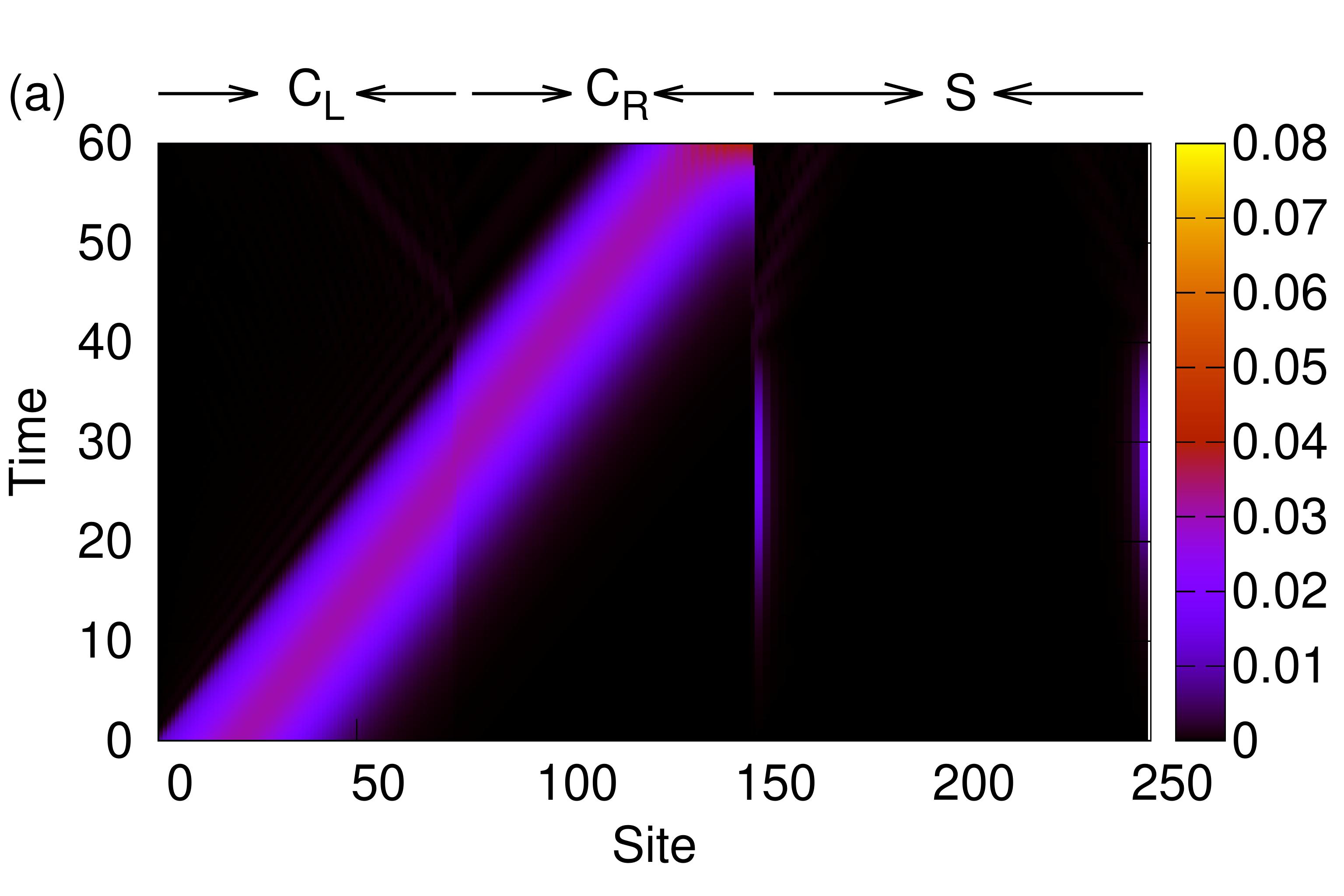
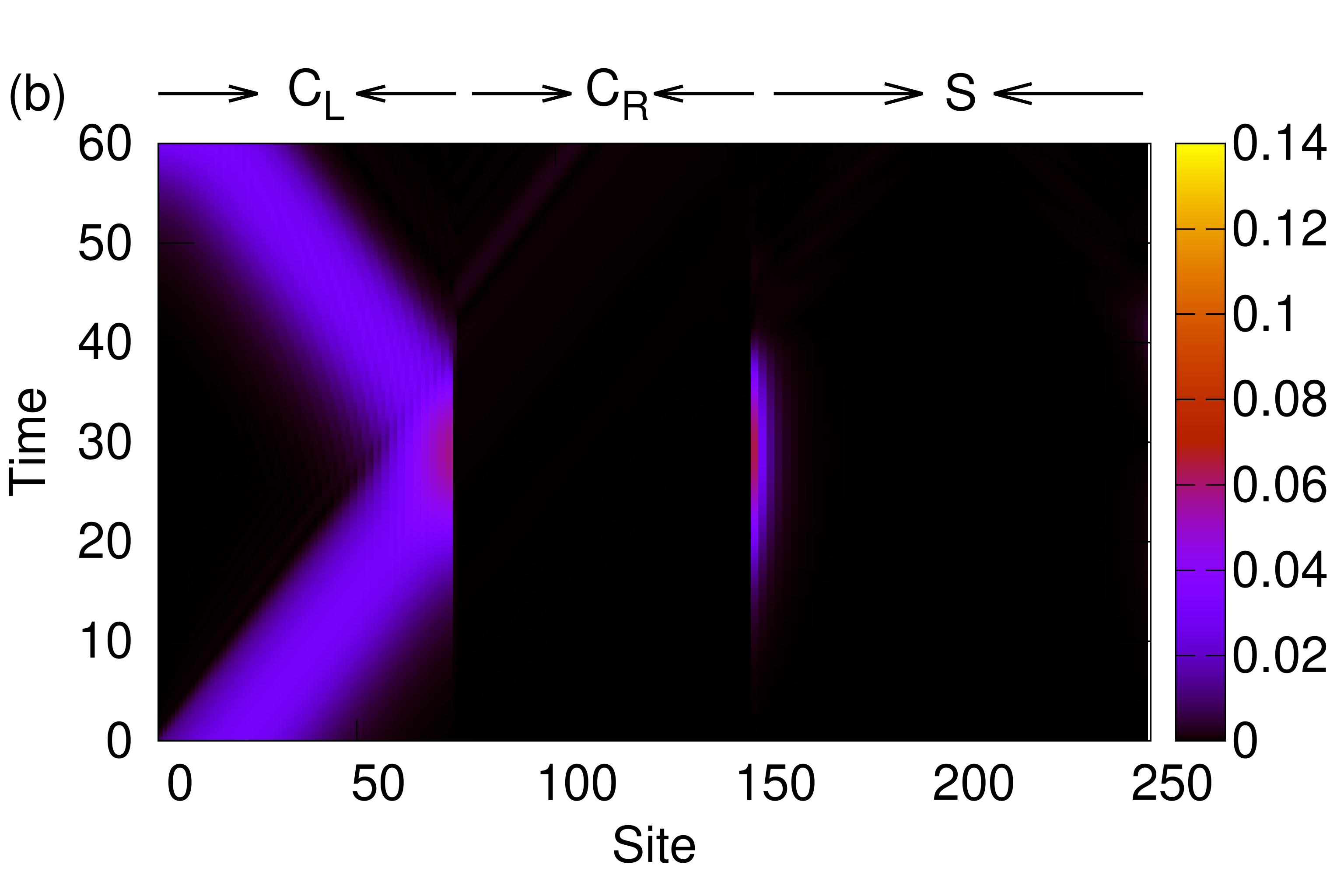
Figure 9: The evolution of the square of the wave amplitude for an incoming wave-packet with energy $E=0$ in the system. The main chain ($site=1,2,\ldots,N_{c}$) with hopping $v=1$ and length $N_{c}=150$ is connected to an open SSH side chain ($site=N_{c}+1,\ldots,N_{c}+N$) of length $N=100$ with couplings $v_{1}=1$, $v_{2}=1$. We mark the left and right parts of the main chain as $C_{L}$ and $C_{R}$ and the SSH side-unit as $S$ for clarity. Here $t=1$. (a) For $t^{\prime}=0.5$ we find perfect transmission and for (b) $t^{\prime}=1.5$ perfect reflection. The wave amplitudes correspond to the two ($*$) symbols shown in Fig. 8.

In Fig. 9(a) and (b) we show the square of the wave amplitude for $t^{\prime}=0.5$ and $t^{\prime}=1.5$, respectively. In the trivial phase ($t^{\prime}<t$), the entire wave-packet is transmitted beyond the scattering region indicating complete transmission. In the topological phase $t^{\prime}>t$ on the other hand, the wave packet is completely reflected from the scattering region. Thus, the dynamics reaffirms the results obtained from TMM, despite the finite energy width of the wavepacket (19). This is enabled by the broad spectral width of the total reflection and total transmission features in Fig. 8 for $t^{\prime}<t$ and $t^{\prime}>t$ respectively.

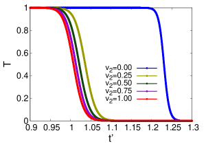
Figure 10: The transmission coefficient as a function of different inter-cell hopping $t^{\prime}$ of the open SSH side chain for different second connection strengths $v_{2}$ with other system parameters fixed at $N=100$, $t=v=v_{1}=1$, $E\sim 0$.

Finally, we show the transmission coefficient as a function of $t^{\prime}$ for different values of $v_{2}$ in Fig. 10. The transmission coefficient shows a step-like drop from $1$ to $0$ as the system switches from the trivial to the topological phase at $t^{\prime}=t$. Usually, this phase transition happens exactly at $t^{\prime}=t$ only for large system sizes. However, Fig. 10 shows that the secondary connection facilitates this phase transition as the jump in $T$ at $t^{\prime}=t$ becomes sharp even for small system sizes. The combination of an energetically broad region of total reflection (for $t^{\prime}<t$) and total transmission (for $t^{\prime}>t$) is evident in Fig. 8, with a fairly abrupt transmission between the two in terms of $t^{\prime}$ as seen in Fig. 10, might have useful switching applications for devices.

IV.3 Case 3: Closed chain with even N

In this subsection we look at the last case, namely the closed SSH chain with an even number of sites. In this scenario, the ends of the side chain are connected to the main chain as well as to each other as shown in Fig. 2. The closed isolated SSH chain becomes gapless at $t^{\prime}=t$ with the two energy bands touching at zero energy as depicted in Fig. 3(c). This results in non-zero energy states in both regions $t^{\prime}<t$ and $t^{\prime}>t$.

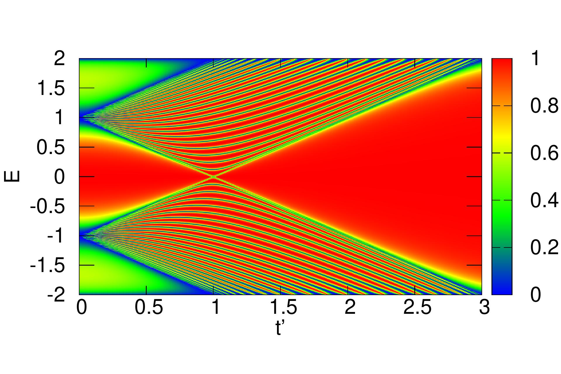
Figure 11: The transmission (T) in the system for various incoming wave energies $E$ and inter-cell couplings $t^{\prime}$ when a single connection exists between the main unit and a closed SSH side unit with length $N=100$. The other parameters are kept constant: $v=1$, $t=1$, $v_{1}=1$, $v_{2}=0$.

Here, the coefficients of the inverse of the matrix $\mathcal{H}_{N}$ are given by $\alpha_{11}=\alpha_{nn}=\frac{\Gamma_{N-1}^{\{1\}}}{\Gamma_{N}}$, $\alpha_{1n}=\alpha_{n1}=\frac{(tt^{\prime})^{\frac{N}{2}}+{t^{\prime}}^{2}\Gamma_{N-2}^{\{1,N\}}}{t^{\prime}{\Gamma_{N}}}$. The relation $\Gamma_{N}=\displaystyle\prod_{\theta_{m}}(E\pm\sqrt{t^{2}+{t^{\prime}}^{2}+2tt^{\prime}\cos\theta_{m}})$ with $\theta_{m}=\frac{4m\pi}{N}$; $m=1,2,\ldots,N/2$ yields $\Gamma_{N}$ [21]. Figure  11 shows the behavior of the transmission coefficient $T$ of the system in the presence of a single connection to the side chain in the two phases ($t^{\prime}>t$ and $t^{\prime}<t$) of the system. Again, perfect transmission is attained for the incoming energies satisfying $\Gamma_{N-1}^{\{1\}}=0$ whereas perfect reflection is attained for energies consistent with $\Gamma_{N}=0$ as shown in Fig. 11. The system shows full transmission for energies close to zero in both the regions ($t^{\prime}>t$ and $t^{\prime}<t$) of the SSH chain due to the opening of the energy bands.

The addition of one more connection ($v_{2}$) further modifies the condition for perfect reflection which now happens for energies consistent with:

$$v\Gamma_{N}+v_{1}v_{2}t^{\prime}\Gamma_{N-2}^{\{1,N\}}+v_{1}v_{2}(t)^{\frac{N}{2}}(t^{\prime})^{\frac{N}{2}-1}=0.$$ (21)

The behavior of the transmission coefficient in the presence of the two adjacent connections to the side chain is shown in Fig. 12.

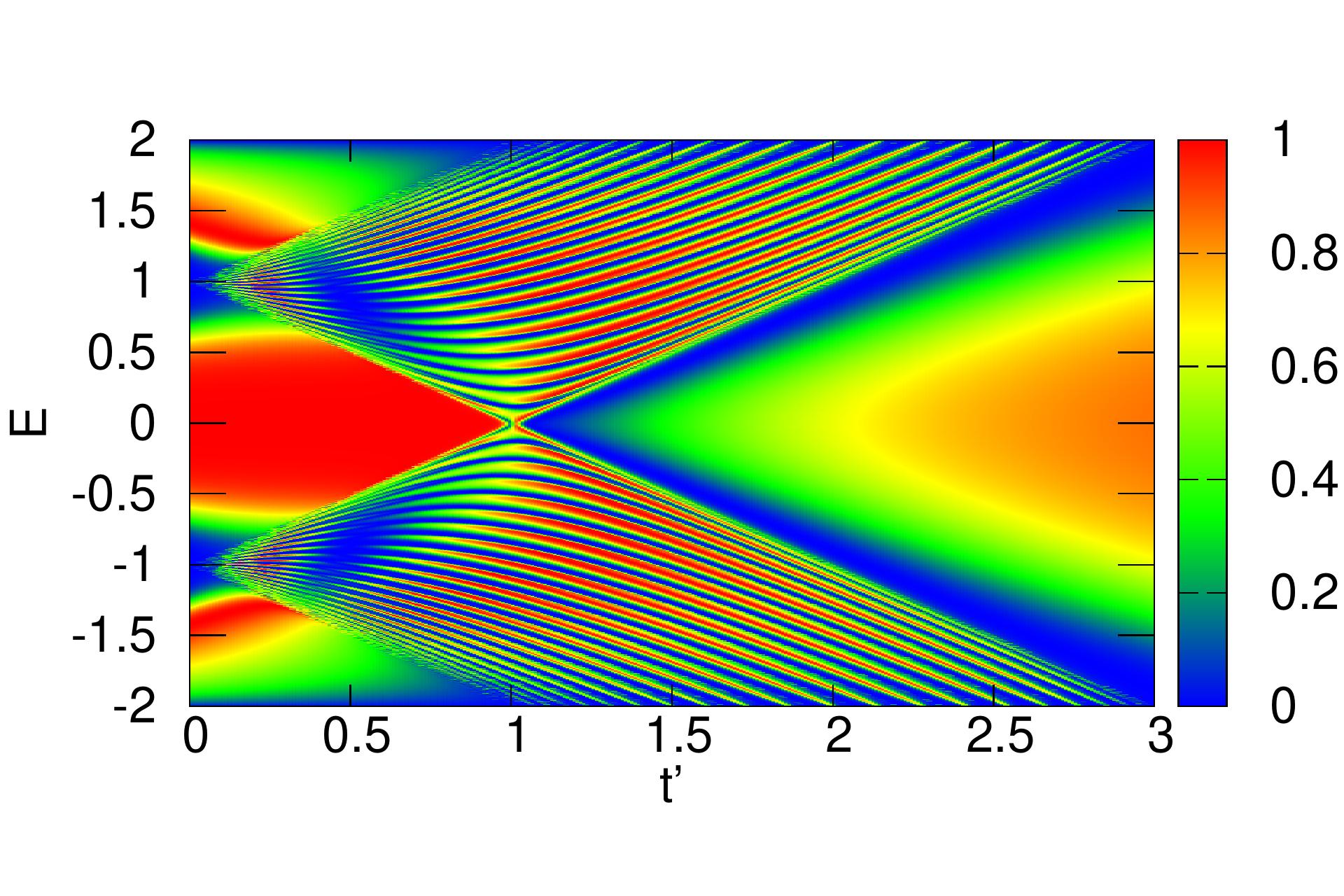
Figure 12: The transmission coefficient $T$ for the closed SSH side chain with $N=100$ for double coupling between the main chain and the side unit. We show $T$ as a function of inter-cell hopping $t^{\prime}$ and incoming wave energy $E$ with other fixed system parameters as $v=1$, $t=1$, $v_{1}=1$, $v_{2}=1$.

The transmission profile exhibits a change from perfect transmission to full reflection in the vicinity of the trivial-to-topological point as featured in Fig. 12. In the extreme case $t^{\prime}\ll t$, the system shows full transmission whereas in the other regime when $t^{\prime}>t$, a suppression of transmission with increasing second coupling strength ($v_{2}$) is seen due to modified reflection conditions given by Eq. (21).

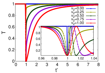
Figure 13: The transmission coefficient as a function of different inter-cell hopping $t^{\prime}$ of the closed SSH side chain for different second connection strengths $v_{2}$. The other system parameters are kept fixed at: $N=100$, $t=v=v_{1}=1$, $E\sim 0$. The inset is a zoomed version that highlights the intricate structure in the vicinity of the phase transition point.

The behavior of the transmission for a range of secondary connection strengths for different inter-leg coupling $t^{\prime}$ is depicted in Fig. 13. In the absence of the second connection $v_{2}$ the transmission coefficient shows a sharp dip at the transition point $t^{\prime}=t$. However, in the presence of the second connection $v_{2}$ the width of the dip at $t^{\prime}=t$ is split into a dip and a peak in the vicinity of the transition point $t^{\prime}=t$. This is due to the extra connection to the main chain which modifies the transmission conditions in the system.

V Experimental Realization

In this section, we briefly discuss the possible experimental realization of our setup. One way to generate the Fano-Anderson chain structures discussed here is using optical lattices filled with ultra cold atoms like Rubidium (${}^{87}Rb$) [22, 23, 24]. For strong lattices, these realize a tight binding chain for the atoms, while when replacing direct tunneling with laser assisted tunneling between some sites, alternating tunneling couplings as required here can be realized [25, 26]. This technique can additionally be combined with employing superlattices [27].

A second platform where our results are directly applicable is photonic crystals [28, 29]. Photonic crystal technology is based on the creation of nanocavities with a photonic band gap [30, 31] which are introduced into a photonic crystal waveguide. These exclusion zones can then practically mimic a tight binding chain for photons, where control over the coupling strengths can be exerted by adjusting the spacing between the sites. Recently, an SSH model with a combination of rigid and elastic materials, which could continuously be tuned across its topological phase transition by stretching  [32] was proposed. By immersing the photonic crystal into a nematic liquid crystal background, dynamical tunability with the help of an external electric field could also be achieved  [33].

VI Conclusion

In this work, we analyse the interplay of Fano resonances, topology and edge states in a Fano-Anderson chain possessing a topological side unit. We take the SSH chain which possesses topological characteristics as a prototype side unit, and show that the topology of the side unit modifies the Fano resonance profile and thus the transport probability past the topological unit. We observe that the transmission profile is modified when the system is tuned from the trivial to the topological phase. With a single connection between the main chain and the side unit, the topological to trivial transition cannot be efficiently detected. However, if two connections are present, a clear signal of the transition is obtained directly from the transmission profile. We provide a detailed study of how the transmission profile depends on the boundary conditions and the topological properties of the SSH chain. The detection of topological characteristics from Fano resonances in quantum transport could allow a new experimental handle on topological states.

We explicitly derive an exact expression for the transmission coefficient using the transfer matrix method and obtain conditions for Fano resonance as well as perfect reflection. The expression obtained can be generalized to an arbitrary side unit and hence may find application in other studies of Fano resonance assisted transport. This enables us to show that an open topological chain with an even number of sites exhibits a sharp transition between complete reflection or complete transmission of all waves with energy near zero, depending on the parameters of the topological scatterer. The sharpness of this transition paired with its wide bandwidth should make this a useful feature for switching in device applications involving photonic crystals or nano-materials with topological elements.

Appendix A Transmission coefficient

We assume that an incoming wave from the far left approaches the scattering region in the main chain and that after the scattering time period, the wave has been split in two parts in the main chain; a reflected part moving towards the left and a transmitted part moving towards the right as shown in Fig. 1(b). The boundary conditions for the stationary scattering states in the time independent scattering problem can be written as:

$$A_{\ell}=I_{0}e^{\iota k\ell}+re^{-\iota k\ell}$$ (22)

for $\ell<1$ and

$$A_{\ell}=t_{out}e^{\iota k\ell}$$ (23)

for $\ell>2$. The coefficients corresponding to the incoming, reflected and transmitted waves are denoted respectively as $I_{0}$, $r$, and $t_{out}$. We can now formulate a transfer matrix that connects the wavefunction on nearby sites of the main chain represented by the lattice equation Eq. (11) as:

$$\begin{bmatrix}&A_{\ell+1}\\ &A_{\ell}\end{bmatrix}=M_{T}\begin{bmatrix}&A_{\ell}\\ &A_{\ell-1}\end{bmatrix},$$ (24)

where $M_{T}$ is the transfer matrix given by

$$M_{T}=\begin{bmatrix}&\frac{E-\alpha_{pp}v^{2}_{1}\delta_{\ell,1}-\alpha_{qq}v^{2}_{2}\delta_{\ell,2}}{v+v_{1}v_{2}\alpha_{pq}\delta_{\ell,1}}&-\frac{v+v_{2}v_{1}\alpha_{qp}\delta_{\ell,2}}{v+v_{1}v_{2}\alpha_{pq}\delta_{\ell,1}}\\ &1&0\end{bmatrix}.$$ (25)

As depicted in Fig. 1, the side unit and main chain are linked by two connections with different hopping $v_{1}$ and $v_{2}$. Hence, we can represent the final transfer matrix of the system as a product of two transfer matrices at the two connecting sites. The first transfer matrix for the connection at the first site $\ell=1$ is given by $M_{1}=(M_{T})_{\ell=1}$ and the second transfer matrix for the connection at the next site $\ell=2$ is given by $M_{2}=(M_{T})_{\ell=2}$. Thus, the final transfer matrix is given by $M=M_{2}M_{1}$ which connects wavefunctions of the parts that lie to the left and right of the scattering regions as

$$\begin{bmatrix}&A_{3}\\ &A_{2}\end{bmatrix}=M\begin{bmatrix}&A_{1}\\ &A_{0}\end{bmatrix}=M_{2}M_{1}\begin{bmatrix}&A_{1}\\ &A_{0}\end{bmatrix}$$ (26)

with

$$M=\begin{bmatrix}&M_{11}&M_{12}\\ &M_{21}&M_{22}\end{bmatrix},$$ (27)

where $M_{ij}=\frac{M^{{}^{\prime}}_{ij}}{v(v+V^{\prime})}$ with $M^{{}^{\prime}}_{11}=[(E-V_{1})(E-V_{2})-|v+V^{\prime}|^{2}]$, $M^{{}^{\prime}}_{12}=-v(E-V_{2})$, $M^{{}^{\prime}}_{21}=v(E-V_{1})$, $M^{{}^{\prime}}_{22}=-v^{2}$. Thus, the final transfer matrix for the setup is given by $M$.

The transmission coefficient $T=|t^{2}_{out}/I_{0}^{2}|$ is calculated from the transfer matrix using the boundary conditions (Eq. (22) and Eq. (23)) as:

$$T=\frac{4\sin^{2}k}{|M_{11}e^{-ik}+M_{12}-M_{21}-M_{22}e^{ik}|^{2}}.$$ (28)

Also, the transmission coefficient in terms of the energy of the incoming wave can be written as:

$$T=\frac{v^{2}(4v^{2}-E^{2})|v+V^{\prime}|^{2}}{[\beta v^{2}+\gamma vE-E^{2}M^{{}^{\prime}}_{11}M^{{}^{\prime}}_{22}]},$$ (29)

where $\beta=(M^{{}^{\prime}}_{11}+M^{{}^{\prime}}_{22})^{2}+(M^{{}^{\prime}}_{12}-M^{{}^{\prime}}_{21})^{2}$ and $\gamma=(M^{{}^{\prime}}_{11}-M^{{}^{\prime}}_{22})(M^{{}^{\prime}}_{12}-M^{{}^{\prime}}_{21})$.

Appendix B Wavefunctions for the edge states

Here, we discuss the eigenstates of the complete Hamiltonian which incorporates the main chain as well as the side SSH chain. The properties of a wave travelling in the main chain with a particular energy are intimately connnected to these eigenstates of the complete Hamiltonian. We focus on the eigenstates corresponding to the energies at which a Fano resonance dip is observed in the transmission profile.

Fig. 14 features the edge states of the system with a single connection ($v_{1}\neq 0$ and $v_{2}=0$) between the main chain and the SSH chain possessing an odd number of sites.

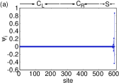
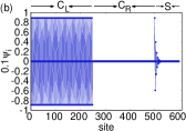
Figure 14: The zero energy wavefunction of the system when the main chain is the simple tight binding chain with length $N_{c}=500$ (corresponding to site indices running from $1$ to $500$) to which an open SSH side chain of length $N=99$ (whose site indices run from $501$ to $599$) is connected to one of the two middle sites. We mark the left and right parts of the main chain as $C_{L}$ and $C_{R}$ and the SSH side-unit as $S$ for clarity. The connecting hopping strengths are $v_{1}=1.0$, $v_{2}=0$ and the other parameters as $v=1.0$, $t=1.0$ with (a) $t^{\prime}=0.5$ and (b) $t^{\prime}=1.5$.

In the region $t^{\prime}<t$, the edge state of the isolated SSH chain lies predominantly on the edge site of the chain and the probability amplitude decays towards the bulk. The state at zero energy of the full system also shows the same behavior as depicted in Fig. 14(a). The eigenstate covers only a few sites close to the free end of the SSH chain and no probability amplitude is seen in the main chain. We would therefore expect no contribution to transport from this eigenstate and thus a very sharp dip is observed in the transmission profile at $E=0$. The eigenstates close to $E=0$ are completely different as they possess probability amplitudes on the main chain (both towards the left and right of the defect) and allow a finite amount of transmission (Fig. 4).

In the region $t^{\prime}>t$, the edge state mainly lies on the connected end of the SSH chain and decays in the bulk of the SSH chain. The connected end shows edge-state character here, despite its connection to the main chain. However, the amplitude at this end of the SSH chain is much smaller than in the other case in Fig. 14(a) which is similar to the the edge state of the isolated SSH chain. Furthermore, as shown in Fig. 14(b), the eigenstate for the full system also shows a finite probability amplitude in the main chain that is to the left of the defect. We take an even total number of sites in the main chain so that the number of sites to the left of the defect is different from the number of sites to the right of the defect, thus breaking the left-right symmetry. As the eigenstate lies merely on one side of the main chain, zero transmission at this energy is observed as depicted in Fig. 4.

Next, we explore the eigenstate of the full system with two connections ($v_{1}\neq 0,\;v_{2}\neq 0$) between the side chain and the main chain ( Fig. 15).

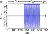
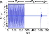
Figure 15: The zero energy wavefunction of the system when the main chain is the simple tight binding chain with $N_{c}=500$ (site indices running from $1$ to $500$) to which an open SSH chain of length $N=99$ (whose site indices run from $501$ to $599$) is connected to one of the middle sites and an adjacent site. The connecting hopping strengths are $v_{1}=1.0$, $v_{2}=1.0$ and the other parameters are $v=1.0$, $t=1.0$, and (a) $t^{\prime}=0.5$ and (b) $t^{\prime}=1.5$.

In Fig. 15 we show the eigenstate corresponding to $E=0$ for both cases $t^{\prime}>t$ and $t^{\prime}<t$. In both cases, the eigenstate of the full system vanishes in one half of the main chain. As a consequence of this, again the transmission in the system is fully suppressed as shown in Fig. 5. With the double coupling, both the ends of the SSH chain are connected to the main chain. We observe that a finite probability amplitude is seen at (a different) one of the edges in the two phases.

The isolated SSH open chain with an even number of sites shows zero modes only when $t^{\prime}>t$, and so we look at the case $t=1.0,t^{\prime}=1.5$. The system now possesses two zero energy states (which are primarily represented at the two edges). Fig. 16 shows the site coefficients of the two zero energy eigenstates for the full Hamiltonian containing the main chain and the side chain, with a single connection $v_{1}$ between them.

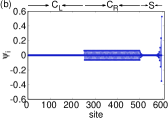
Figure 16: The wavefunction for the two zero energy states with a simple tight binding chain with $N_{c}=500$ (site indices running from $1$ to $500$) as main chain and an open SSH chain with $N=100$ (site indices running from $501$ to $600$) as a side chain which is connected to one of the middle sites. The connecting hopping strengths are $v_{1}=1.0$, $v_{2}=0$ and other parameters are $v=1.0$, $t=1.0$ and $t^{\prime}=1.5$.

We observe that both these states possess a finite probability amplitude one part of the main chain and also at the free end of the SSH chain as shown in Fig. 16. The zero amplitude of the eigenstate in one half of the main chain confirms the full reflection in the system corresponding to this energy as depicted in Fig. 7.

The presence of the second connection $v_{2}$ leaves no free end for the SSH chain. Thus, the eigenstate for the full system is modified as shown in Fig. 17.

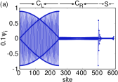
Figure 17: The wavefunction for the two zero energy states for system consisting of a simple tight binding chain with $N_{c}=500$ (site indices running from $1$ to $500$) as main chain and an open SSH chain with $N=100$ (site indices running from $501$ to $600$) as side chain which is connected to one of the middle sites and an adjacent site. The connecting hopping strengths are $v_{1}=1.0$, $v_{2}=1.0$ and the other parameters are $v=1.0$, $t=1.0$ and $t^{\prime}=1.5$.

The majority of the probability amplitude lies on the one half of the main chain which results in zero transport in the system as depicted in Fig. 8.

Appendix C Nearest neighbor tight binding open chain as side unit

We consider a nearest neighbour tight binding chain with hopping $t$ (i.e., $t=t^{\prime}$) coupled to the main chain with two connections $v_{1}$ and $v_{2}$.

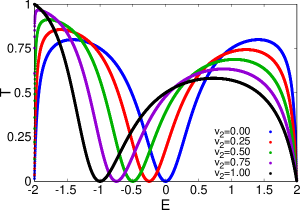
Figure 18: Transmission coefficient as a function of the incoming wave energy with various second connection strengths $v_{2}$ when the main chain is the simple tight binding chain and the side unit is a single site. The parameters are $v=1.0$, $v_{1}=1.0$, $t=1.0$.

The transmission coefficient ($T$) as a function of incoming wave energies ($E$) is shown in Fig. 18 and Fig. 19 for different secondary connection strength $v_{2}$ when the sideunit possesses one ($N=1$) and two ($N=2$) sites respectively.

In the absence of $v_{2}$, the system shows a minimum transmission ($T=0$) at $E=0$ when the side unit contains an odd number of sites as the condition $\Gamma_{N}=0$ is satisfied. For even number of sites in the side chain, the system shows a maximum transmission ($T=1$) at $E=0$ as the condition $\Gamma_{N-1}^{\{1\}}=0$ is satisfied.

In the presence of the second connection $v_{2}$, the perfect reflection condition is given by:

$$v\Gamma_{N}+v_{1}v_{2}t^{N-1}=0,$$ (30)

where $\Gamma_{N}=\displaystyle\prod_{k}(E-2t\cos(k))$ with $k=\frac{j\pi}{N+1}$; $j=1,\ldots,N$ with $N$ being the side chain length.

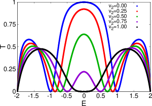
Figure 19: Transmission coefficient as a function of incoming wave energy with various second connection strengths $v_{2}$ when the main chain is the simple tight binding chain and the side unit is a two-site chain. The other parameters are $v=1.0$, $v_{1}=1.0$, $t=1.0$.

If a single defect site is connected to the main chain through two connections $v_{1}$ and $v_{2}$ then the position of the minimum of transmission is shifted by $-v_{2}$ ( Fig. 18) according to Eq. (30). Again invoking (30) for $N=2$, as $v_{2}$ is increased, the minima at $E=\pm 1$ move towards each other as shown in Fig. 19. Thus, the maximum at $E=0$ for $v_{2}=0$ turns into a minimum for $v_{2}=1$.

References

- [1] Ugo Fano. Sullo spettro di assorbimento dei gas nobili presso il limite dello spettro d’arco. Il Nuovo Cimento, 12(3):154–161, 1935.
- [2] Ugo Fano. Effects of configuration interaction on intensities and phase shifts. Phys. Rev., 124(6):1866, 1961.
- [3] Andrey E Miroshnichenko, Sergej Flach, and Yuri S Kivshar. Fano resonances in nanoscale structures. Reviews of Modern Physics, 82(3):2257, 2010.
- [4] O Újsághy, J Kroha, L Szunyogh, and A Zawadowski. Theory of the fano resonance in the stm tunneling density of states due to a single kondo impurity. Physical review letters, 85(12):2557, 2000.
- [5] Stefan Rotter, Florian Libisch, Joachim Burgdörfer, U Kuhl, and H-J Stöckmann. Tunable fano resonances in transport through microwave billiards. Physical Review E, 69(4):046208, 2004.
- [6] A Attaran, SD Emami, MRK Soltanian, R Penny, SW Harun, H Ahmad, HA Abdul-Rashid, M Moghavvemi, et al. Circuit model of fano resonance on tetramers, pentamers, and broken symmetry pentamers. Plasmonics, 9(6):1303–1313, 2014.
- [7] Pengyu Fan, Zongfu Yu, Shanhui Fan, and Mark L Brongersma. Optical fano resonance of an individual semiconductor nanostructure. Nature materials, 13(5):471–475, 2014.
- [8] Christos Argyropoulos, Francesco Monticone, Giuseppe D’Aguanno, and Andrea Alù. Plasmonic nanoparticles and metasurfaces to realize fano spectra at ultraviolet wavelengths. Applied Physics Letters, 103(14):143113, 2013.
- [9] Farbod Shafiei, Francesco Monticone, Khai Q Le, Xing-Xiang Liu, Thomas Hartsfield, Andrea Alù, and Xiaoqin Li. A subwavelength plasmonic metamolecule exhibiting magnetic-based optical fano resonance. Nature nanotechnology, 8(2):95, 2013.
- [10] Ajith Ramachandran, Carlo Danieli, and Sergej Flach. Fano resonances in flat band networks. In Fano Resonances in Optics and Microwaves, pages 311–329. Springer, 2018.
- [11] Andrey E Miroshnichenko and Yuri S Kivshar. Engineering fano resonances in discrete arrays. Physical Review E, 72(5):056611, 2005.
- [12] Stefano Longhi. Bound states in the continuum in a single-level fano-anderson model. The European Physical Journal B, 57(1):45–51, 2007.
- [13] Evgeny N Bulgakov and Almas F Sadreev. Resonance induced by a bound state in the continuum in a two-level nonlinear fano-anderson model. Physical Review B, 80(11):115308, 2009.
- [14] Arunava Chakrabarti. Fano resonance in discrete lattice models: Controlling lineshapes with impurities. Physics Letters A, 366(4-5):507–512, 2007.
- [15] Arunava Chakrabarti. Electronic transmission in a model quantum wire with side-coupled quasiperiodic chains: Fano resonance and related issues. Physical Review B, 74(20):205315, 2006.
- [16] Ling Lu, John D Joannopoulos, and Marin Soljačić. Topological photonics. Nature photonics, 8(11):821, 2014.
- [17] P St-Jean, V Goblot, E Galopin, A Lemaître, T Ozawa, L Le Gratiet, I Sagnes, J Bloch, and A Amo. Lasing in topological edge states of a one-dimensional lattice. Nature Photonics, 11(10):651–656, 2017.
- [18] Farzad Zangeneh-Nejad and Romain Fleury. Topological fano resonances. Physical review letters, 122(1):014301, 2019.
- [19] Peiqing Tong, Baowen Li, and Bambi Hu. Wave transmission, phonon localization, and heat conduction of a one-dimensional frenkel-kontorova chain. Phys. Rev. B, 59:8639–8645, Apr 1999.
- [20] Joan R Westlake. A handbook of numerical matrix inversion and solution of linear equations, volume 767. Wiley New York, 1968.
- [21] J Sirker, M Maiti, NP Konstantinidis, and N Sedlmayr. Boundary fidelity and entanglement in the symmetry protected topological phase of the ssh model. Journal of Statistical Mechanics: Theory and Experiment, 2014(10):P10032, 2014.
- [22] Matthias Theis. Optical Feshbach resonances in a Bose-Einstein condensate. na, 2005.
- [23] Sebastian Krinner, Tilman Esslinger, and Jean-Philippe Brantut. Two-terminal transport measurements with cold atoms. Journal of Physics: Condensed Matter, 29(34):343003, 2017.
- [24] Christian Gross and Immanuel Bloch. Quantum simulations with ultracold atoms in optical lattices. Science, 357(6355):995–1001, 2017.
- [25] Hirokazu Miyake, Georgios A. Siviloglou, Colin J. Kennedy, William Cody Burton, and Wolfgang Ketterle. Realizing the harper hamiltonian with laser-assisted tunneling in optical lattices. Phys. Rev. Lett., 111:185302, Oct 2013.
- [26] M. Aidelsburger, M. Atala, M. Lohse, J. T. Barreiro, B. Paredes, and I. Bloch. Realization of the hofstadter hamiltonian with ultracold atoms in optical lattices. Phys. Rev. Lett., 111:185301, Oct 2013.
- [27] Fabrice Gerbier and Jean Dalibard. Gauge fields for ultracold atoms in optical superlattices. New Journal of Physics, 12(3):033007, mar 2010.
- [28] Kuon Inoue and Kazuo Ohtaka. Photonic crystals: physics, fabrication and applications, volume 94. Springer Science & Business Media, 2004.
- [29] Su-Peng Yu, Juan A. Muniz, Chen-Lung Hung, and H. J. Kimble. Two-dimensional photonic crystals for engineering atom–light interactions. Proceedings of the National Academy of Sciences, 116(26):12743–12751, 2019.
- [30] Eiichi Kuramochi. Manipulating and trapping light with photonic crystals from fundamental studies to practical applications. Journal of Materials Chemistry C, 4(47):11032–11049, 2016.
- [31] Kurt Busch, Sergei F Mingaleev, Antonio Garcia-Martin, Matthias Schillinger, and Daniel Hermann. The wannier function approach to photonic crystal circuits. Journal of Physics: Condensed Matter, 15(30):R1233, 2003.
- [32] Ehsan Saei Ghareh Naz, Ion Cosma Fulga, Libo Ma, Oliver G Schmidt, and Jeroen van den Brink. Topological phase transition in a stretchable photonic crystal. Physical Review A, 98(3):033830, 2018.
- [33] Mikhail I Shalaev, Sameerah Desnavi, Wiktor Walasik, and Natalia M Litchinitser. Reconfigurable topological photonic crystal. New Journal of Physics, 20(2):023040, 2018.