Note on the pairwise interactions of surfactant-covered drops in a uniform electric field

Abstract

We study the effect of surfactant on the pairwise interactions of drops in an applied uniform DC electric field using a combination of numerical simulations based on a boundary integral formulation and an analytical theory assuming small drop deformations. The surfactant is assumed to be insoluble in the bulk-phase fluids. We show that the surfactant weakens the electrohydrodynamic flow and thus dielectrophoretic interactions play more prominent role in the dynamics of surfactant-covered drops compared to clean drops. If drop conductivity is the same as the suspending fluid, a nondiffusing surfactant can arrest the drops’ relative motion thereby effectively preventing coalescence.

I Introduction

Electric fields are widely used to manipulate particles and fluids. For example, separation of emulsified water from crude oil in the petroleum refining process is achieved by the application of electric fields, which facilitate drop coalescence (Waterman, 1965; Eow and Ghadiri, 2002). An important question pertains to the influence of surface-active substances (surfactants, compounds that lower the surface tension between liquids), which are naturally present in the crude oil (asphaltenes, resins, acids), on the process droplet attraction and coalescence.

The effect of surfactants and electric fields on drop dynamics has been largely studied in two-dimensions, whilst in three-dimensions the literature is limited. The effect of surfactant (no electric field) has been studied using simulations based on the boundary integral method (Li and Pozrikidis, 1997; Pozrikidis, 2004; Stone and Leal, 1990; Yon and Pozrikidis, 1998; Eggleton et al., 2001; Bazhlekov et al., 2006; Feigl et al., 2007; Vlahovska et al., 2005; Rother et al., 2006), the diffuse-interface-method (Teigen et al., 2011), a front-tracking method (Muradoglu and Tryggvason, 2008) or a conserving volume-of-fluid method (James and Lowengrub, 2004). The effect of electric fields on clean drops (no surfactant) has been studied theoretically, numerically and experimentally both for single and multiple drops (Lac and Homsy, 2007; Karyappa et al., 2014; Lanauze et al., 2015; Ha and Yang, 2015; Das and Saintillan, 2017; Fernandez, 2008; Casas et al., 2019; Baygents et al., 1998; Lin et al., 2012; Mhatre et al., 2015; LSalipante et al., 2010; Sozou, 1975; Zabarankin, 2020), and we refer the interested reader to our recent work (Sorgentone et al., 2020) for a more extensive bibliography. In that paper we presented a detailed analysis of the three-dimensional interaction of a drop pair in a uniform electric field; we showed that the pair dynamics are not simple attraction or repulsion; depending on the angle between the center-to-center line with the undisturbed electric field, the relative motion of the two particles can be quite complex. For example, they can attract in the direction of the field and move towards each other, pair up, and then separate in the transverse direction.

The combined effect of surfactants and electric fields is a virtually unexplored problem in terms of numerical experiments, especially when considering multiple drops. This is due to the numerous computational challenges associated with the complex moving geometries and the multi-physics nature of the problem. Teigen and Munkejord used a level-set method in an axisymmetric, cylindrical coordinate system to investigate the interaction between surfactant-covered drops with a uniform electric field for a single drop and, more recently, Poddar et al., studied theoretically the electrorheology of a dilute emulsion of surfactant-covered drops (Poddar et al., 2019). Other theoretical studies developed asymptotic analyses (Ha and Yang, 1995; Nganguia et al., 2013, 2019) to investigate the deformation and the effects of surfactant transport on the deformation of a single viscous drop under a DC electric field.

In this note we built upon our previous work (Sorgentone et al., 2019, 2020) and explore the effect of an insoluble surfactant on a drop pair electrohydrodynamics.

II Problem formulation

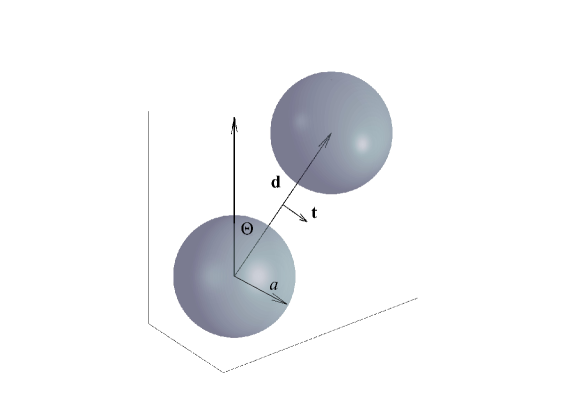
Figure 1: Two initially spherical identical drops with radius $a$, permittivity ${\varepsilon}_{\mathrm{d}}$ and conductivity $\sigma_{\mathrm{d}}$ suspended in a fluid permittivity ${\varepsilon}_{\mathrm{s}}$ and conductivity $\sigma_{\mathrm{s}}$ and subjected to a uniform DC electric field ${\bf E}^{\infty}=E_{0}{\bf\hat{z}}$. The angle between the line-of-centers vector and the field direction is $\Theta=\arccos({\bf\hat{z}}\cdot{\bf\hat{d}})$.

Let us consider two identical neutrally-buoyant and charge-free drops with radius $a$, viscosity $\eta_{\mathrm{d}}$, conductivity $\sigma_{\mathrm{d}}$, and permittivity ${\varepsilon}_{\mathrm{d}}$ suspended in a fluid with viscosity $\eta_{\mathrm{s}}$, conductivity $\sigma_{\mathrm{s}}$, and permittivity ${\varepsilon}_{\mathrm{s}}$. The mismatch in drop and suspending fluid properties is characterized by the conductivity, permittivity, and viscosity ratios

$$\mbox{\it R}=\frac{\sigma_{\mathrm{d}}}{\sigma_{\mathrm{s}}}\,,\quad\mbox{\it S}=\frac{{\varepsilon}_{\mathrm{d}}}{{\varepsilon}_{\mathrm{s}}}\,,\quad\lambda=\frac{\eta_{\mathrm{d}}}{\eta_{\mathrm{s}}}\,.$$ (1)

A monolayer of insoluble surfactant is adsorbed on the drop interfaces. At rest, the surfactant distribution is uniform and the equilibrium surfactant concentration is $\Gamma_{\mathrm{eq}}$; the corresponding interfacial tension is $\gamma_{\mathrm{eq}}$. The distance between the drops’ centroids is $d$ and the angle between the drops’ line-of-centers with the applied field direction is $\Theta$. The unit separation vector between the drops is defined by the difference between the position vectors of the drops’ centers of mass ${\bf\hat{d}}=({\bf x}_{2}^{c}-{\bf x}^{c}_{1})/d$. The unit vector normal to the drops line-of-centers and orthogonal to ${\bf\hat{d}}$ is ${\bf{\hat{t}}}$. The problem geometry is sketched in Figure 1.

We adopt the leaky dielectric model (Melcher and Taylor, 1969), which assumes creeping flow and charge-free bulk fluids acting as Ohmic conductors. The assumption of charge-free fluids decouples the electric and hydrodynamic fields in the bulk. Accordingly,

$$\eta\nabla^{2}{\bm{u}}-\nabla p=0\,,\quad\nabla\cdot{\bf E}=0\,,$$ (2)

where ${\bm{u}}$ and $p$ are the fluid velocity and pressure, and ${\bf E}$ is the electric field. Far away from the drops, ${\bf E}^{\mathrm{s}}\rightarrow{\bf E}^{\infty}=E_{0}{\bf\hat{z}}$ and ${\bm{u}}\rightarrow 0$.

The coupling of the electric field and the fluid flow occurs at the drop interfaces $\cal{D}$, where the charges brought by conduction accumulate. The Gauss’ law dictates that while the electric field in the electroneutral bulk fluids is solenoidal, at the drop interface the electric displacement field, ${\varepsilon}{\bf E}$, is discontinuous and its jump corresponds to the surface charge density

$${\varepsilon}\left(E_{n}^{\mathrm{s}}-\mbox{\it S}E_{n}^{\mathrm{d}}\right)=q\,,\quad{\bf x}\in\cal{D}$$ (3)

where $E_{n}={\bf E}\cdot{\bf n}$, and ${\bf n}$ is the outward pointing normal vector to the drop interface. The surface charge density adjusts to satisfy the current balance

$$\frac{\partial q}{\partial t}+\nabla_{s}\cdot\left({\bm{u}}q\right)=\sigma_{\mathrm{s}}\left(E_{n}^{\mathrm{s}}-\mbox{\it R}E_{n}^{\mathrm{d}}\right)\,,\quad{\bf x}\in\cal{D}\,.$$ (4)

In this study, we neglect charge relaxation and convection, thereby reducing the charge conservation equation to continuity of the electrical current across the interface as originally proposed by Taylor (1966)

$$E_{n}^{\mathrm{s}}=\mbox{\it R}E_{n}^{\mathrm{d}}\,.$$ (5)

This simplification implies ${\varepsilon}^{2}_{\mathrm{s}}E_{0}^{2}/(\eta_{\mathrm{s}}\sigma_{\mathrm{s}})\ll 1$. This condition is satisfied for the typical fluids used in experiments such as castor oil (conductivity is $\sim 10^{-11}$ S/m, viscosity is $\sim 1$ Pa.s) and low field strengths $E_{0}\sim 10^{4}$ V/m.

The electric field acting on the induced surface charge gives rise to electric shear stress at the interface. The tangential stress balance yields

$$\left({\bf I}-{\bf n}{\bf n}\right)\cdot\left({\bf T}^{\mathrm{s}}-{\bf T}^{\mathrm{d}}\right)\cdot{\bf n}+q{\bf E}_{t}=-{\bm{\nabla}}_{s}\gamma\,,\quad{\bf x}\in\cal{D}\,,$$ (6)

where $T_{ij}=-p\delta_{ij}+\eta(\partial_{j}u_{i}+\partial_{i}u_{j})$ is the hydrodynamic stress and $\delta_{ij}$ is the Kronecker delta function. The electric tractions is calculated from the Maxwell stress tensor $T^{\mathrm{el}}_{ij}={\varepsilon}\left(E_{i}E_{j}-E_{k}E_{k}\delta_{ij}/2\right)$. $\gamma$ is the interfacial tension, which depends on the local surfactant concentration $\Gamma$. ${\bf E}_{t}={\bf E}-E_{n}{\bf n}$ is the tangential component of the electric field, which is continuous across the interface, and ${\bf I}$ is the idemfactor. The normal stress balance is

$${\bf n}\cdot\left({\bf T}^{\mathrm{s}}-{\bf T}^{\mathrm{d}}\right)+\frac{1}{2}\left(\left(E_{n}^{{\mathrm{s}}}\right)^{2}-\mbox{\it S}\left(E_{n}^{{\mathrm{d}}}\right)^{2}-(1-\mbox{\it S})E_{t}^{2}\right)=\gamma\,\nabla_{s}\cdot{\bf n}\,,\quad{\bf x}\in\cal{D}\,,$$ (7)

concentration $\Gamma$.

The evolution of the distribution of an insoluble, diffusing surfactant is governed by a time-dependent convective equation (Stone, 1990; Wong et al., 1996)

$$\frac{\partial\Gamma}{\partial t}+{\bm{\nabla}}_{\mathrm{s}}\cdot\left({\bm{u}}_{\mathrm{s}}\Gamma\right)+\Gamma\left({\bm{u}}\cdot{\bf n}\right)\nabla_{\mathrm{s}}\cdot{\bf n}-D\nabla^{2}_{s}\Gamma=0\,\quad{\mbox{at}}\quad r=r_{s}\,$$ (8)

where ${\bm{\nabla}}_{\mathrm{s}}$ is the surface gradient operator, ${\bm{\nabla}}_{\mathrm{s}}=\left({\bf I}-{\bf n}{\bf n}\right)\cdot{\bm{\nabla}}$.

We adopt a linear equation of state for the interfacial tension

$$\gamma(\Gamma)=\gamma_{\mathrm{eq}}-\left.\frac{\partial\gamma}{\partial\Gamma}\right|_{\mathrm{eq}}\,\left(\Gamma-\Gamma_{\mathrm{eq}}\right).$$ (9)

Henceforth, all variables are nondimensionalized using the radius of the undeformed drops $a$, the undisturbed field strength $E_{0}$, a characteristic applied stress $\tau_{c}={\varepsilon}_{\mathrm{s}}E_{0}^{2}$, and the properties of the suspending fluid. Accordingly, the time scale is $t_{c}=\eta_{\mathrm{s}}/\tau_{c}$ and the velocity scale is $u_{c}=a\tau_{c}/\eta_{\mathrm{s}}$. The surfactant concentration is normalized by $\Gamma_{\mathrm{eq}}$ and the interfacial tension - by $\gamma_{\mathrm{eq}}$. The ratio of the magnitude of the electric stresses and surface tension defines the electric capillary number, the relative strength of the distorting viscous and restoring Marangoni stresses is reflected by the Marangoni number and the importance of surfactant diffusion is given by the Peclet number

$$\mbox{\it Ca}=\frac{{\varepsilon}_{\mathrm{s}}E_{0}^{2}a}{\gamma_{\mathrm{eq}}}\,,\quad\mbox{\it Ma\,}^{-1}=\frac{{\varepsilon}_{\mathrm{s}}E_{0}^{2}a}{\Delta\gamma}\,,\quad\mbox{\it Pe}=\frac{{\varepsilon}_{\mathrm{s}}E_{0}^{2}a^{2}}{\eta_{\mathrm{s}}D}\,.$$ (10)

The characteristic magnitude of the surface-tension variations that result from perturbations of the local surfactant concentration $\Gamma$ about the equilibrium value $\Gamma_{\mathrm{eq}}$ is

$$\Delta\gamma=-\Gamma_{\rm eq}\left(\frac{\partial\gamma}{\partial\Gamma}\right)_{\Gamma=\Gamma_{\rm eq}}$$

It is convenient to define the elasticity number, which is independent of the externally applied stresses

$$\mbox{\it E}=\frac{\gamma_{0}-\gamma_{\mathrm{eq}}}{\gamma_{\mathrm{eq}}}=\mbox{\it Ca}\mbox{\it Ma\,}\,.$$ (11)

III Numerical method

We utilize the boundary integral method to solve for the flow and electric fields. Details of our three-dimensional formulation can be found in (Sorgentone et al., 2019). In brief, the electric field is computed following (Lac and Homsy, 2007; Baygents et al., 1998):

$${\bf E}^{\infty}+\sum_{j=1}^{2}\int_{{\cal{D}}_{j}}\frac{\hat{{\bf x}}}{4\pi r^{3}}{\left({\bf E}^{\mathrm{s}}-{\bf E}^{\mathrm{d}}\right)\cdot{\bf n}}dS({\bf y})=\begin{cases}{\bf E}^{\mathrm{d}}({\bf x})&\mbox{if }{\bf x}$ inside $\cal{D},\\ \frac{1}{2}\left({\bf E}^{\mathrm{d}}({\bf x})+{\bf E}^{\mathrm{s}}({\bf x})\right)&\mbox{if }{\bf x}\in\cal{D},\\ {\bf E}^{\mathrm{s}}({\bf x})&\mbox{if }{\bf x}$ outside $\cal{D}.\\ \end{cases}$$ (12)

where ${\bf\hat{x}}={\bf x}-{\bf y}$ and $r=|{\bf\hat{x}}|$. The normal and tangential components of the electric field are calculated from the above equation

$$\begin{split}E_{n}({\bf x})&=\frac{2\mbox{\it R}}{\mbox{\it R}+1}{\bf E}^{\infty}\cdot{\bf n}+\frac{\mbox{\it R}-1}{\mbox{\it R}+1}\sum_{j=1}^{2}{\bf n}({\bf x})\cdot\int_{{\cal{D}}_{j}}\frac{{\bf\hat{x}}}{2\pi r^{3}}E_{n}({\bf y})dS({\bf y})\,,\\ {\bf E}_{t}({\bf x})&=\frac{{\bf E}^{\mathrm{s}}+{\bf E}^{\mathrm{d}}}{2}-\frac{1+\mbox{\it R}}{2\mbox{\it R}}E_{n}{\bf n}\,.\end{split}$$ (13)

For the flow field, we have developed the method for fluids of arbitrary viscosity, but for the sake of brevity here we list the equation in the case of equiviscous drops and suspending fluids. The velocity is given by

$$2{\bm{u}}({\bf x})=-\sum_{j=1}^{2}\left(\frac{1}{4\pi}\int_{{\cal{D}}_{j}}\left(\frac{{\bf f}({\bf y})}{\mbox{\it Ca}}-{\bf f}^{E}({\bf y})\right)\cdot\left(\frac{{\bf I}}{r}+\frac{{\bf\hat{x}}{\bf\hat{x}}}{r^{3}}\right)dS({\bf y})\right)\,,$$ (14)

where ${\bf f}$ and ${\bf f}^{E}$ are the interfacial stresses due to surface tension and electric field

$${\bf f}=\gamma({\bf x}){\bf n}\nabla\cdot{\bf n}-{\bm{\nabla}}_{\mathrm{s}}\gamma\,,$$ (15)

$${\bf f}^{E}=\left({\bf E}^{\mathrm{s}}\cdot{\bf n}\right){\bf E}^{\mathrm{s}}-\frac{1}{2}\left({\bf E}^{\mathrm{s}}\cdot{\bf E}^{\mathrm{s}}\right){\bf n}-\mbox{\it S}\left(\left({\bf E}^{\mathrm{d}}\cdot{\bf n}\right){\bf E}^{\mathrm{d}}-\frac{1}{2}\left({\bf E}^{\mathrm{d}}\cdot{\bf E}^{\mathrm{d}}\right){\bf n}\right)\,.$$ (16)

For a clean drop, the surface tension coefficient $\gamma({\bf x})$ will be constant, and the second term in (15), the so-called Marangoni force, will vanish.
Drop velocity and centroid are computed from the volume averages

$${\bf U}_{j}=\frac{1}{V}\int_{V_{j}}{\bm{u}}dV=\frac{1}{V}\int_{{\cal{D}}_{j}}{\bf n}\cdot\left({\bm{u}}{\bf x}\right)dS\,,\quad{\bf x}^{c}_{j}=\frac{1}{V}\int_{V_{j}}{\bf x}dV=\frac{1}{2V}\int_{{\cal{D}}_{j}}{\bf n}\left({\bf x}\cdot{\bf x}\right)dS\,.$$ (17)

To solve the system of equations Eq. (13), Eq. (14), Eq. (8) we use the Galerkin formulation based on a spherical harmonics representation presented in Sorgentone et al. (2019). In the current study, we update the time scheme to the adaptive fourth order Runge-Kutta introduced in Kennedy and Carpenter (2003). This choice allows to treat the convective term that appear in the surfactant evolution equation Eq. (8) explicitely, and the diffusive term implicitely. To make the implicit part of the solver efficient also for large diffusion coefficients (i.e. Small Péclet numbers), a preconditioner designed in (Pålsson et al., 2017) results to be fundamental to reduce the number of iterations for the convergence. All variables (position vector, velocities, electric field, surfactant concentration etc) are expanded in spherical harmonics which provides an accurate representation even for relatively low expansion order. In this respect, to make sure that all the geometrical quantities of interest (e.g. mean curvature) are computed with high accuracy as well, we use the adaptive upsampling procedure proposed by Rahimian et al. (2015). A specialized quadrature method for the singular and nearly singular integrals that appear in the formulation and a reparametrization procedure able to ensure a high-quality representation of the drops also under deformation are used to ensure the spectral accuracy of the method (Sorgentone and Tornberg, 2018).

Our numerical method and the asymptotic theory for clean drops was presented and validated in (Sorgentone et al., 2020). Here we extend the small-deformation theory and the numerical method to include the effect of the insoluble surfactant.

IV Theory: Far-field interactions

We first analyze the electrostatic interaction of two widely separated spherical drops. In this case, the drops can be approximated by point-dipoles. The disturbance field ${\bf E}_{1}$ of the drop dipole ${\bf P}_{1}$ induces a dielectrophoretic (DEP) force on the dipole ${\bf P}_{2}$ located at ${\bf x}^{c}_{2}=d{\bf\hat{d}}$, given by ${\bf F}(d)=\left({\bf P}_{2}\cdot\nabla{\bf E}_{1}\right)|_{r=d}$ The drop velocity under the action of this force can be estimated from Stokes law, ${\bf U}={\bf F}/\zeta$, where $\zeta$ is the friction coefficient. For a surfactant-covered drop, $\zeta=6\pi(3\lambda+2+\chi)/(3(\lambda+1)+\chi)$, where $\chi=\mbox{\it Pe}\mbox{\it Ma\,}$. Thus,

$${\bf U}_{2}^{\mathrm{dep}}=2\frac{\beta_{D}}{d^{4}}\left(\frac{\chi+3(1+{\lambda})}{\chi+2+3{\lambda}}\right)\left[\left(1-3\cos^{2}\Theta\right){\bf\hat{d}}-\sin\left(2\Theta\right){\bf{\hat{t}}}\right]\,,\quad\beta_{D}=\left(\frac{\mbox{\it R}-1}{\mbox{\it R}+2}\right)^{2}$$ (18)

The velocity reduces to the result for clean drops if $\chi=0$ Sorgentone et al. (2020), and for solid spheres if $\chi\rightarrow\infty$.

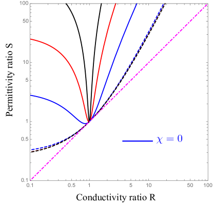
Figure 2: (a) Phase diagram of drop deformations and alignment with the field for viscosity ratio ${\lambda}=1$ and different values of the parameter $\chi=\mbox{\it Pe}\mbox{\it Ma\,}$. The solid lines correspond to $\Phi_{s}({\lambda},\mbox{\it R},\mbox{\it S},\chi)=0$ given by Eq. (26); in the parameter space above, the line of centers of the two drops rotates away from the applied field direction $\Phi<0$. The dashed lines correspond to the modified Taylor discriminating function Eq. (33); in the parameter space above it, drop deformation is oblate and below it - prolate. Above the dot-dashed magenta line $\mbox{\it S}=\mbox{\it R}$, the surface flow is pole-to-equator ($\beta<0$), while below this line the surface flow is equator-to-pole ($\beta>0$)

In addition to the dipole-dipole interaction, drops interact hydrodynamically. Assuming a spherical drop, the electric shear drives a flow, which is a combination of a stresslet and a quadrupole Taylor (1966)

$${\bm{u}}=\frac{\beta}{r^{2}}\left(-1+3\cos^{2}\theta\right){\bf\hat{r}}-\frac{\beta}{r^{4}}\left(\left(-1+3\cos^{2}\theta\right){\bf\hat{r}}+\sin(2\theta){\bm{\hat{}}\theta}\right)\,.$$ (19)

The strength of the stresslet is

$$\beta=\beta_{T}-\frac{3\mbox{\it Ma\,}}{5(1+{\lambda})}g\,,\quad\beta_{T}=\frac{9}{10}\frac{\mbox{\it R}-\mbox{\it S}}{\left(1+\lambda\right)\left(\mbox{\it R}+2\right)^{2}}\,,$$ (20)

where $g$ is a parameter describing the surfactant redistribution, $\Gamma=1+g\left(-1+3\cos^{2}\theta\right)$. The surfactant weakens the EHD flow, because the Marangoni stresses due to nonuniform surfactant concentration oppose the shearing electric traction. At steady state, the surfactant distribution at leading order is given by the balance of surfactant convection by the electrohydrodynamic (EHD) flow and surfactant diffusion, $\nabla_{s}\cdot{\bm{u}}=\mbox{\it Pe}^{-1}\nabla^{2}\Gamma$, which leads to

$$g=\mbox{\it Pe}\frac{5(1+{\lambda})}{3\left(5(1+{\lambda})+\chi\right)}\beta_{T}\,,$$ (21)

and thus

$$\beta=\frac{9\left(\mbox{\it R}-\mbox{\it S}\right)}{2\left(\mbox{\it R}+1\right)^{2}}\frac{1}{5(1+{\lambda})+\chi}\,,\quad\chi=\mbox{\it Pe}\mbox{\it Ma\,}\,.$$ (22)

The parameter $\chi$ characterizes the magnitude of the surfactant effect on the EHD flow. In the limit $\chi=0$ the result reduces to the clean drop solution. In the case of nondiffusing surfactant $\mbox{\it Pe}\rightarrow\infty$ ($\chi\rightarrow\infty$), the surfactant completely immobilizes the interface and suppresses the EHD flow. In this case, the theory predicts that the drops will interact only electrostatically. Moreover, if $\mbox{\it R}=1$ even the DEP interaction vanishes. Thus a pair of spherical droplets covered with insoluble, nondiffusing surfactant and conductivity ratio $\mbox{\it R}=1$ will not interact in a uniform electric field.

The drop translational velocity due to a neighbor drop is found from Faxen’s law (Kim and Karrila, 1991; Pak et al., 2014)

$${{\bf U}}^{\mathrm{ehd}}_{2}=\left(1+\frac{\lambda}{2(3\lambda+2)}\nabla^{2}\right){\bm{u}}|_{{\bf x}=d{\bf\hat{d}}}\,.$$ (23)

Inserting Eq. (19) in the above equation leads to

$${{\bf U}}^{\mathrm{ehd}}_{2}=\beta\left(\frac{1}{d^{2}}-\frac{2}{d^{4}}\left(\frac{1+3{\lambda}}{2+3{\lambda}}\right)\right)\left(-1+3\cos^{2}\Theta\right){\bf\hat{d}}-\frac{2\beta}{d^{4}}\left(\frac{1+3{\lambda}}{2+3{\lambda}}\right)\sin(2\Theta){\bf{\hat{t}}}+O(d^{-5})\,.$$ (24)

Combining the electrohydrodynamic and the dielectrophoretic velocities yields

$${\bf U}_{2}=\frac{\beta}{d^{2}}\left(-1+3\cos^{2}\Theta\right){\bf\hat{d}}-\Phi_{s}\left({\lambda},\mbox{\it R},\mbox{\it S},\chi\right)\frac{2}{d^{4}}\left(\left(-1+3\cos^{2}\theta\right){\bf\hat{d}}+\sin(2\Theta){\bf{\hat{t}}}\right)\,,$$ (25)

where

$$\Phi_{s}=\frac{1+3{\lambda}}{2+3{\lambda}}\beta+\beta_{D}\frac{3(1+{\lambda})+\chi}{2+3{\lambda}+\chi}\,.$$ (26)

The discriminant ${\Phi_{s}}$ quantifies the drop pair alignment with the field and the interplay of EHD and DEP interactions in drop attraction or repulsion. Drops with $\Phi_{s}>0$ move to align their line-of-centers to with the applied electric field, since $\dot{\Theta}={\bf U}_{2}\cdot{\bf{\hat{t}}}\sim-\Phi_{s}$. If $\Phi_{s}<0$ (which occurs only for $\mbox{\it R}/\mbox{\it S}<1$ drops), the line of centers between the drops rotates towards a perpendicular orientation with respect to the applied electric field. The presence of surfactant reduces the parameter range where misalignment is predicted. Figure 2 summarizes the regimes of alignment and deformation.

The relative radial motion of the two drops at a given separation depends on $\Phi_{s}$ and $\beta_{T}$. There is a critical separation $d_{c}$ corresponding to ${\bf U}_{2}(d_{c})\cdot{\bf\hat{d}}=0$ at which drop relative radial motion can change sign

$$d_{c}^{2}=\frac{2(1+3{\lambda})}{2+3{\lambda}}+\frac{\left(\mbox{\it R}-1\right)^{2}}{\mbox{\it R}-\mbox{\it S}}\left(\frac{4(3(1+{\lambda})+\chi)(5(1+{\lambda})+\chi)}{9(2+3{\lambda}+\chi)}\right).$$ (27)

For $\Phi_{s}>0$ and $\mbox{\it R}/\mbox{\it S}<1$ ($\beta<0)$, $d_{c}$ does not exist and EHD and DEP interactions are cooperative and act in the same direction (note that system with $\Phi_{s}<0$ and $\mbox{\it R}/\mbox{\it S}>1$ can not exist). For $\Phi_{s}>0$ and $\mbox{\it R}/\mbox{\it S}>1$ or $\Phi_{s}<0$ and $\mbox{\it R}/\mbox{\it S}<1$, there is competition between EHD and DEP, with the quadrupolar DEP winning out closer to the drops and the EHD taking over via the stresslet flow in the far-field. The critical distance is affected by the presence of surfactant. It increases with $\chi$, since the surfactant weakens the EHD flow and expands the region of dominance of DEP. In the limit of nondiffusing surfactant, $\chi\rightarrow\infty$, the drop interactions are entirely dominated by DEP.

V Results and discussion

We consider two identical drops with viscosity ratio ${\lambda}=1$ and focus on the effect of surfactant on drop dynamics under variable R, S and initial configuration.

First we compare the drop steady velocity obtained from simulations and the asymptotic theory for a drop pair aligned with the field. Figure 3 shows that theory and simulations are in excellent agreement, especially at large separations, and the theory is able to capture the steady velocity even for a relatively high $\mbox{\it Ca}=1$. As the surfactant effect strengthens and $\chi$ increases, either by increase in the surfactant elasticity or decreasing diffusivity, the drops relative velocity switches from EHD to DEP dominated at the critical distance Eq. (27). Accordingly the slope dependence on distance changes from $d^{-2}$ to $d^{-4}$. This is most obvious for the $\chi=100$ case, where $d_{c}=7.14$. In the limit $\chi\rightarrow\infty$, the drop motion is entirely due to DEP.

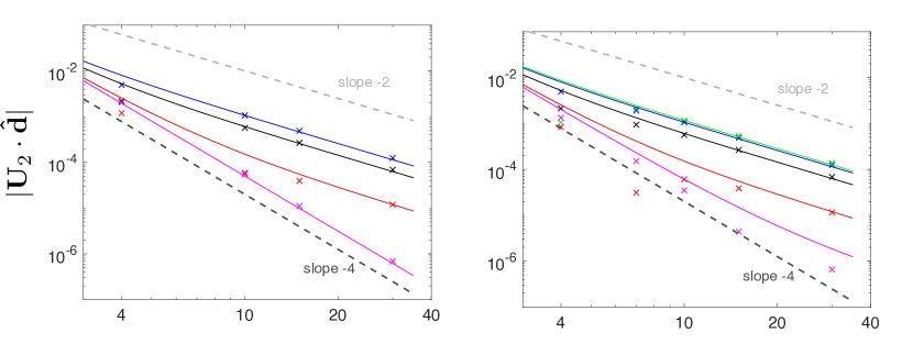
Figure 3: Steady relative velocity of a pair of leaky dielectric drops aligned with the field ($\Theta=0$). $\mbox{\it R}=2$, $\mbox{\it S}=1$, $\mbox{\it Ca}=1$ (left) $\mbox{\it E}=1$, $\mbox{\it Pe}=1$ (blue),$\mbox{\it Pe}=10$ (black) ,$\mbox{\it Pe}=100$ (red) and $\mbox{\it Pe}\rightarrow\infty$(magenta). The symbols are from our fully 3D code and the solid line is the theory Eq. (25). In the case of nondiffusing surfactant the interaction is dominated by DEP and the velocity shows $1/d^{4}$ dependence. (right) $\mbox{\it Pe}=1$ and $\mbox{\it E}=0,1,10,100,1000$ (green, blue, black, red, magenta). As $\chi=\mbox{\it Ma\,}\mbox{\it Pe}$ increases the critical distance beyond which the DEP dominates increases. Note that $\chi=100$ shows change of slope from -4 and -2. $\chi=1000$ slope -4 in the studied range.

However, even in this limit where at steady state the interface is immobilized by the surfactant, until the steady DEP-dominated state is reached, there is EHD affected drop motion due to the transient drop deformation and surfactant redistribution. As a result, the drops can initially repel and then attract once steady drop shape and surfactant distribution are reached. This scenario is illustrated on Figure 4, which shows that the radial relative velocity in the case of a drop covered with non-diffusing surfactant can change sign from positive (indicating drop repulsion) to negative (attraction). The small-deformation theory which predicts this phenomenon is presented in the Appendix.

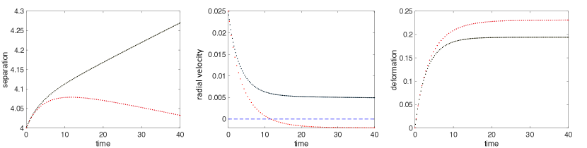
Figure 4: Effect of surfactant on the interaction of two identical drops with $\mbox{\it R}=2$, $\mbox{\it S}=1$, $\mbox{\it Ca}=1$, $\mbox{\it E}=1$ initially aligned with the field $\Theta=0$. Black dots correspond to $\mbox{\it Pe}=1$ and red dots correspond to the limit of non-diffusing surfactant $\mbox{\it Pe}=10^{6}$. The surfactant suppresses the electrohydrodynamic repulsion and after initial transient due to shape deformation and surfactant redistribution the interaction can reverse sign.

Our previous study of clean drops (Sorgentone et al., 2020) found that drops initially misaligned with the field may not experience monotonic attraction or repulsion; instead their three-dimensional trajectories follow three scenarios: motion in the direction of the field accompanied by either attraction followed by separation or vice versa (repulsion followed by attraction), and attraction followed by separation in a direction transverse to the field. Next we address the question about the surfactant influence on these intricate dynamics. The theory presented in Figure 2 highlighted that the surfactant has two main effects: first, it increases the range of distances where DEP dominates over EHD, and second, decreases the range of S and R parameters where drops’ line-of-centers rotates away from the direction of the applied field. Accordingly, clean and surfactant-covered drops with same S and R, initial configuration and Ca may display opposite aligning behavior. Figure 5 illustrates such a case. While the clean drops attract in the direction of the field and move towards each other, pair up, and then separate in the transverse direction, the surfactant-covered drops only attract and move to align their line-of-centers parallel to the field.

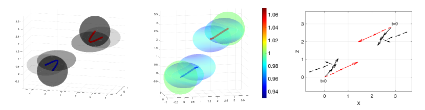
Figure 5: $\mbox{\it R}=0.1,\mbox{\it S}=5,\Theta=45\textdegree$. Initial distance $d=4$.(a) clean drops misaligning (b) non-diffusing surfactant-covered drops with $\mbox{\it E}=10$ aligning with the field (c) Center of mass trajectory in the $x-z$ plane. Arrows correspond to the velocity for the clean drops (black) and for the non-diffusing surfactant-covered drops (red). Movies in the additional material.

VI Conclusions

The effect of surfactant on the three-dimensional interactions of a drop pair in an applied electric field is studied using numerical simulations and a small-deformation theory based on the the leaky dielectric model. We present results for the case of a uniform electric field and arbitrary angle between the drops’ line-of-centers and the applied field direction, where the non-axisymmetric geometry necessitates three-dimensional simulations.

The surfactant’s main effect is to decrease the electrohydrodynamic flow due to Marangoni stresses compensating the electric shear. As a result, drops’ interactions are more strongly affected by DEP: the surfactant-covered drops tend to align with the applied field direction and attract. The surfactant influence is quantified by the parameter $\chi=\mbox{\it Pe}\mbox{\it Ma\,}$. The surfactant effect is most pronounced for nondiffusing surfactant ($\mbox{\it Pe}\gg 1$) or high elasticity $\mbox{\it Ma\,}\gg 1$. The critical separation at which the DEP overcomes the EHD interaction increases with $\chi$. The interaction is much weaker compared to the clean drops, because DEP decays with the drops’ separation as $1/d^{4}$ compared to the $1/d^{2}$ for EHD. The DEP also causes drops to align with the field and the range of R and S where the drops attract and move in the direction of the field and then separate in the transverse direction is greatly diminished.

VII Acknowledgments

PV has been supported in part by NSF award CBET-1704996.

Appendix A Electrohydrodynamic velocity of a surfactant-covered drop with transient deformation

Let us consider drop dynamics upon the application of an uniform electric field in the limit of small deformations $\mbox{\it Ca}\ll 1$. At leading order in Ca, the shape and surfactant concentration are described by $r_{s}=1+f(t)\left(-1+3\cos^{2}\theta\right)$ and $\Gamma=1+g(t)\left(-1+3\cos^{2}\theta\right)$. The deformation parameter is $D=3/2f$. Combining the small-deformation theories for a surfactant-covered drop in applied flow Vlahovska et al. (2009); Vlahovska (2016) and electric field Vlahovska (2011, 2019) yields

$$\dot{f}=\frac{1}{(3+2{\lambda})(16+19{\lambda})}\left[15(1+{\lambda})t_{n}^{\mathrm{el}}+9(2+3{\lambda})t_{t}^{\mathrm{el}}-\mbox{\it Ca}^{-1}\left(4f(10(1+{\lambda})+\beta(4+{\lambda}))-2\beta g(4+{\lambda})\right)\right]$$ (28)

$$\begin{split}\dot{g}=&\frac{1}{(3+2{\lambda})(16+19{\lambda})}\left[9(2+3{\lambda})t_{n}^{\mathrm{el}}+9(12+13{\lambda})t_{t}^{\mathrm{el}}-\mbox{\it Ca}^{-1}\left(12f\left(2(2+3{\lambda})-\beta(8+7{\lambda})\right)+6\beta g(8+7{\lambda})\right)\right]\\ &+\mbox{\it Pe}^{-1}6(g-2f)\end{split}$$ (29)

where

$$t^{e}_{n}=\frac{1+\mbox{\it R}^{2}-2\mbox{\it S}}{(\mbox{\it R}+2)^{2}}\,,\quad t^{e}_{t}=\frac{\mbox{\it R}-\mbox{\it S}}{\left(\mbox{\it R}+2\right)^{2}}$$ (30)

Steady state deformation depends on the parameter $\chi=\beta\mbox{\it Pe}/\mbox{\it Ca}$

$$f=\frac{3\mbox{\it Ca}}{8}F_{S}\left(\mbox{\it R},\mbox{\it S},{\lambda},\chi\right)\,,$$ (31)

where Ha and Yang (1995)

$$\begin{split}F_{S}\left(\mbox{\it R},\mbox{\it S},{\lambda},\chi\right)=&\frac{1}{\left(2+\mbox{\it R}\right)^{2}}\left(\mbox{\it R}^{2}+1-2\mbox{\it S}+\left(\mbox{\it R}-\mbox{\it S}\right)\frac{3\left(2+3{\lambda}\right)+2\chi}{5({\lambda}+1)+\chi}\right)\,,\end{split}$$ (32)

The limit $\chi=0$ recovers the result for a clean drop $f_{clean}=3F_{T}/8$, where $F_{T}$ is the Taylor discriminating function

$$\begin{split}F_{T}\left(\mbox{\it R},\mbox{\it S},{\lambda}\right)=&\frac{1}{\left(2+\mbox{\it R}\right)^{2}}\left(\mbox{\it R}^{2}+1-2\mbox{\it S}+3\left(\mbox{\it R}-\mbox{\it S}\right)\frac{2+3{\lambda}}{5({\lambda}+1)}\right)\,,\end{split}$$ (33)

The limit $\chi\rightarrow\infty$ recovers insoluble surfactant resultNganguia et al. (2013)

$$f=\frac{3}{8}\mbox{\it Ca}\frac{\left(\mbox{\it R}+1\right)^{2}-4\mbox{\it S}}{\left(\mbox{\it R}+2\right)^{2}}$$ (34)

The velocity field outside the drop at distance $r$ from the drop center and an angle $\theta$ with the applied field direction is given by (Vlahovska, 2016)

$${\bm{u}}=\left(\frac{\alpha+\beta}{r^{2}}-\frac{\beta}{r^{4}}\right)\left(-1+3\cos^{2}\theta\right){\bf\hat{r}}-\frac{\beta}{r^{4}}\sin(2\theta){\bm{\hat{}}\theta}\,,$$ (35)

where

$$\begin{split}\alpha=&\frac{15({\lambda}+1)}{(3+2{\lambda})(16+19{\lambda})}\left(F_{T}\left(\mbox{\it R},\mbox{\it S},{\lambda}\right)-\mbox{\it Ca}^{-1}\left(\frac{8}{3}f_{2}(t)+\mbox{\it E}\frac{2(4+{\lambda})}{15(1+{\lambda})}\left(-2f_{2}(t)+g_{2}(t)\right)\right)\right)\\ \beta=&\frac{1)}{(3+2{\lambda})(16+19{\lambda})}\left(B_{T}\left(\mbox{\it R},\mbox{\it S},{\lambda}\right)-\mbox{\it Ca}^{-1}\left(12(2+3{\lambda})f_{2}(t)+\mbox{\it E}\left(8+7{\lambda}\right)\left(-2f_{2}(t)+g_{2}(t)\right)\right))\right)\,.\end{split}$$ (36)

where

$$\begin{split}B_{T}\left(\mbox{\it R},\mbox{\it S},{\lambda}\right)=&\frac{9\left({\lambda}\left(3\mbox{\it R}^{2}+13\mbox{\it R}-19\mbox{\it S}+3\right)+2\left(\mbox{\it R}^{2}+6\mbox{\it R}-8\mbox{\it S}+1\right)\right)}{2(\mbox{\it R}+2)^{2}}\,.\end{split}$$ (37)

The shape evolution equation is obtained from the kinematic condition $\dot{r}_{s}=u_{r}(r=1)$. The surfactant evolution is obtained from $\dot{\Gamma}=-\nabla_{s}\cdot{\bm{u}}+\mbox{\it Pe}^{-1}\nabla_{s}^{2}\Gamma$.

If a second drop is present at location ${\bf x}_{2}^{c}=d{\bf\hat{d}}$, its migration velocity due to the electrohydrodynamic flow of the first drop can be obtained using Faxen’s law (Kim and Karrila, 1991)

$${{\bf U}}_{2}^{{\mathrm{ehd}}}=\left(1+\frac{{\lambda}}{2(3{\lambda}+2)}\nabla^{2}\right){\bm{u}}({r=d}).$$ (38)

Inserting Eq. (35) in the above equation yields

$$\begin{split}U_{2,r}^{\mathrm{ehd}}&=\left(\frac{\alpha+\beta}{r^{2}}-\frac{1}{r^{4}}\left(\beta+\frac{3{\lambda}}{2+3{\lambda}}\left(\alpha+\beta\right)\right)\right)\left(-1+3\cos^{2}\theta\right)\\ U_{2,\theta}^{\mathrm{ehd}}&=-\frac{1}{r^{4}}\left(\beta+\frac{3{\lambda}}{2+3{\lambda}}\left(\alpha+\beta\right)\right)\sin(2\theta)\end{split}$$ (39)

At steady state $\alpha=0$ and $\beta$ reduces to the result for a spherical drop Eq. (24).

Figure 6 shows the evolution of the radial and tangential velocity and compares the theory with the numerical simulation.

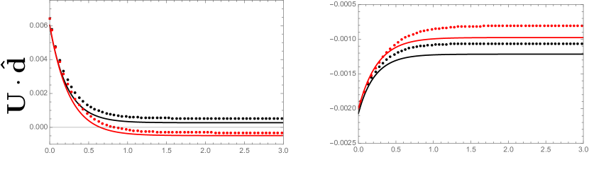
Figure 6: Evolution of the relative radial (left) and tangential (right) velocities for a drop pair with $\mbox{\it R}=2\,,\,\mbox{\it S}=1$. Initial angle $\Theta=45\textdegree$ and distance $d=4$. Symbols are numerical simulations and line is the theory. $\chi=1$ (black) and $\chi=10^{6}$ (red). Note that the relative radial velocity changes sign for $\chi=10^{6}$ indicating change from repulsion to attraction. In both cases drops move to aline their line-of-centers with the applied field direction.

Appendix B 3D trajectories of surfactant-covered drops in a uniform electric field

Next we illustrate the pair dynamics at different initial configurations. Our previous work showed that clean drops can undergo complex dynamics in an applied uniform electric field if they are initially misaligned with the field: repulsion followed by attraction with centerline rotating towards the applied field direction (a) and (d), attraction followed by repulsion with centerline rotating towards the applied field direction (c), and attraction followed by repulsion with centerline rotating away from the applied field direction (b). The drops remain in the plane defined by the initial separation vector and the applied field direction, in this case the $xz$ plane. The transient pairing dynamics are clearly seen in the trajectories in the $xz$ plane. Figures 7-8 show that in these cases the surfactant does not qualitatively change the dynamics, even though the surfactant concentration does become nonuniform.

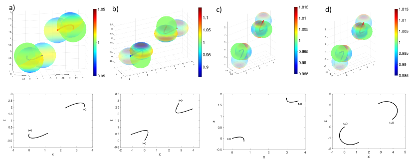
Figure 7: Trajectories of two identical surfactant-covered drops with (a) $\mbox{\it R}=0.1$, $\mbox{\it S}=1$, (b) $\mbox{\it R}=1$, $\mbox{\it S}=10$, (c) $\mbox{\it R}=1$, $\mbox{\it S}=0.1$ and (d) $\mbox{\it R}=100$, $\mbox{\it S}=1$. Initially the drops are in the xz plane, the separation in all cases is $d=4$ and the angle with the applied field direction is (a) $\Theta=60^{o}$, (b) $\Theta=45^{o}$, (c) $\Theta=65^{o}$, and (d) $\Theta=80^{o}$. $\mbox{\it Ca}=0.1$, $\mbox{\it E}=1$ and $\mbox{\it Pe}=10^{6}$. Bottom: trajectories in the xz planes. The color map shows the surfactant concentration

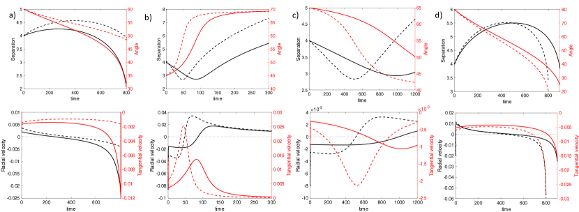
Figure 8: Dynamics of a pair of identical drops with initial separation $d=4$ and different angles with the applied field. Comparison between clean (dotted line) and surfactant-covered drops (solid line) with $\mbox{\it E}=1$ and $\mbox{\it Pe}=10^{6}$. $\mbox{\it Ca}=0.1$. (a) R=0.1, S=1 (repulsion-attraction, alignment with the field), (b)R=1, S=10 (attraction-repulsion, misalignment with the field), (c) R=1, S=0.1 (attraction-repulsion, alignment perpendicular to the field), and (d) R=100, S=1 (repulsion-attraction, alignment with the field).

References

- Waterman [1965] L. C. Waterman. Electric coalescers. Chem. Eng. Prog., 61:51–57, 1965.
- Eow and Ghadiri [2002] J. S. Eow and M. Ghadiri. Electrostatic enhancement of coalescence of water droplets in oil: a review of the technology. Chem. Eng. Sci., 85:357–368, 2002.
- Li and Pozrikidis [1997] X. Li and C. Pozrikidis. The effect of surfactants on drop deformation and on the rheology of dilute emulsions in Stokes flow. J. Fluid Mech., 341:165–194, 1997.
- Pozrikidis [2004] C. Pozrikidis. A finite-element method for interfacial surfactant transport, with application to the flow-induced deformation of a viscous drop. J. Eng. Math., 49:163–180, 2004.
- Stone and Leal [1990] H. A. Stone and L. G. Leal. The effects of surfactants on drop deformation and breakup. J. Fluid Mech., 220:161–186, 1990.
- Yon and Pozrikidis [1998] S. Yon and C. Pozrikidis. A finite-volume/boundary-element method for flow past interfaces in the presence of surfactants, with application to shear flow past a viscous drop. Computers Fluids, 27:879–902, 1998.
- Eggleton et al. [2001] C.D. Eggleton, T.M. Tsai, and K.J. Stebe. Tip streaming from a drop in the presence of surfactants. PRL, 87:048302, 2001.
- Bazhlekov et al. [2006] I. B. Bazhlekov, P. D. Anderson, and H. E. H. Meijer. Numerical investigation of the effect of insoluble surfactants on drop deformation and breakup in simple shear flow. J. Coll. Int. Sci., 298:369–394, 2006.
- Feigl et al. [2007] K. Feigl, D. Megias-Alguacil, P. Fischer, and E.J Windhab. Simulation and experiments of droplet deformation and orientation in simple shear flow with surfactants. Chem. Eng. Sci., 62:3242–3258, 2007.
- Vlahovska et al. [2005] P. Vlahovska, J. Bławzdziewicz, and M. Loewenberg. Deformation of a surfactant-covered drop in a linear flow. Phys. Fluids, 17:Art. No.103103, 2005.
- Rother et al. [2006] M. A. Rother, A. Z. Zinchenko, and R. H. Davis. Surfactant effects on buoyancy-driven viscous interactions of deformable drops. Coll. Surf. A, 282:50–60, 2006.
- Teigen et al. [2011] Knut Erik Teigen, Peng Song, John Lowengrub, and Axel Voigt. A diffuse-interface method for two-phase flows with soluble surfactants. J. Comp. Phys., 230:375–393, 2011.
- Muradoglu and Tryggvason [2008] M. Muradoglu and G. Tryggvason. A front-tracking method for computation of interfacial flows with soluble surfactants. J. Comp. Phys., 227:2238–2262, 2008.
- James and Lowengrub [2004] A. J. James and J. Lowengrub. A surfactant-conserving volume-of-fluid method for interfacial flows with insoluble surfactant. J. Comp. Phys., 201:685–722, 2004.
- Lac and Homsy [2007] E. Lac and G. M. Homsy. Axisymmetric deformation and stability of a viscous drop in a steady electric field. J. Fluid. Mech, 590:239–264, 2007.
- Karyappa et al. [2014] R. B. Karyappa, S. D. Deshmukh, and R. M. Thaokar. Breakup of aconducting drop in a uniform electric field. J. Fluid Mech., 754: 550-589, 2014.
- Lanauze et al. [2015] J.A. Lanauze, L. M. Walker, and A. S. Khair. Nonlinear electrohydrodynamics of slightly deformed oblate drops . J. Fluid Mech., 774:245-266, 2015.
- Ha and Yang [2015] J.-W. Ha and S.-M. Yang. Rheological responses of oil-in-oil emulsions in an electric field. J. Rheol., 44:235-256, 2000.
- Das and Saintillan [2017] D. Das and D. Saintillan. Electrohydrodynamics of viscous drops in strong electric fields: numerical simulations. J. Fluid. Mech, 829:127-152, 2017.
- Fernandez [2008] A. Fernandez. Response of an emulsion of leaky dielectric drops immersed in a simple shear flow: Drops more conductive than the suspending fluid. Phys. Fluids, 20 2008.
- Casas et al. [2019] P.S. Casas, M. Garzon, L.J. Gray, and J.. Sethian. Numerical study on electro- hydrodynamic multiple droplet interactions. Phys. Rev. E 100, 100 2019.
- Baygents et al. [1998] J. C. Baygents, N. J. Rivette, and H. A. Stone. Electrohydrodynamic deformation and interaction of drop pairs. J. Fluid. Mech., 368:359–375, 1998.
- Lin et al. [2012] Y. Lin, P. Skjetne, and A. Carlson. A phase field model for multiphase electro-hydrodynamic flow. International Journal of Multiphase Flow, 45:1-11, 2012.
- Mhatre et al. [2015] S. Mhatre, S. Deshmukh, and R. Thaokar. Electrocoalescence of a drop pair. Physics of Fluids, 27(9), 2015.
- LSalipante et al. [2010] P.F. Salipante, P. F. and P.M. Vlahovska Electrohydrodynamics of drops in strong uniform dc electric fields. IPhys. Fluids, 22, 2010.
- Sozou [1975] C. Sozou. Electrohydrodynamics of a pair of liquid drops. Journal of Fluid Mechanics, 67(2):339-348, 1975.
- Zabarankin [2020] M. Zabarankin. mall deformation theory for two leaky dielectric drops in a uniform electric field. JProc. Royal Soc. A , 476, 2020.
- Sorgentone et al. [2020] C. Sorgentone, J. Kach, A. Khair, L. Walker, and Petia M. Vlahovska. Electrohydrodynamic interactions of drop pairs. J. Fluid Mech., page accepted, 2020.
- Poddar et al. [2019] Antarip Poddar, Shubhadeep Mandal, Aditya Bandopadhyay, and Suman Chakraborty. Electrorheology of a dilute emulsion of surfactant-covered drops. Journal of Fluid Mechanics, 881:524?550, 2019. doi: 10.1017/jfm.2019.745.
- Ha and Yang [1995] J. W. Ha and S. M. Yang. Effects of surfactant on the deformation and stability of a drop in a viscous fluid in an electric field. J.Coll. Int. Sci., 175:369–385, 1995.
- Nganguia et al. [2013] H. Nganguia, Y. N. Young, P. M. Vlahovska, J. Blawzdziewcz, J. Zhang, and H. Lin. Equilibrium electro-deformation of a surfactant-laden viscous drop. Phys. Fluids, 25:092106, 2013.
- Nganguia et al. [2019] Herve Nganguia, On Shun Pak, and Y.-N. Young. Effects of surfactant transport on electrodeformation of a viscous drop. Phys. Rev. E, 99:063104, Jun 2019. doi: 10.1103/PhysRevE.99.063104. URL https://link.aps.org/doi/10.1103/PhysRevE.99.063104.
- Sorgentone et al. [2019] C. Sorgentone, A.-K. Tornberg, and Petia M. Vlahovska. A 3D boundary integral method for the electrohydrodynamics of surfactant-covered drops. J. Comp. Phys., 389: 111–127, 2019.
- Melcher and Taylor [1969] J. R. Melcher and G. I. Taylor. Electrohydrodynamics - a review of role of interfacial shear stress. Annu. Rev. Fluid Mech., 1:111–146, 1969.
- Taylor [1966] G. I. Taylor. Studies in electrohydrodynamics. I. Circulation produced in a drop by an electric field. Proc. Royal Soc. A, 291:159–166, 1966.
- Stone [1990] H. A. Stone. A simple derivation of the time-dependent convective-diffusion equation for surfactant transport along a deforming interface. Phys. Fluids A, 2:111–112, 1990.
- Wong et al. [1996] Harris Wong, David Rumschitzki, and Charles Maldarelli. On the surfactant mass balance at a deforming fluid interface. Physics of Fluids, 8(11):3203–3204, 1996. doi: 10.1063/1.869098. URL https://doi.org/10.1063/1.869098.
- Kennedy and Carpenter [2003] Christopher A. Kennedy and Mark H. Carpenter. Additive runge–kutta schemes for convection–diffusion–reaction equations. Applied Numerical Mathematics, 44(1):139 – 181, 2003. ISSN 0168-9274. doi: https://doi.org/10.1016/S0168-9274(02)00138-1. URL http://www.sciencedirect.com/science/article/pii/S0168927402001381.
- Pålsson et al. [2017] Sara Pålsson, Chiara Sorgentone, and Anna-Karin Tornberg. Adaptive time-stepping for surfactant-laden drops. D.J. Chappel (Ed.), on Boundary Integral Method (UKBIM11), Nottingham Trent University: Publications, Nottingham, pages 161 – 170, 2017.
- Rahimian et al. [2015] A. Rahimian, S.K. Veerapaneni, D. Zorin, and G. Biros. Boundary integral method for the flow of vescicles with viscosity contrast in three dimensions. Journal of Computational Physics, 298:766–786, 2015.
- Sorgentone and Tornberg [2018] C. Sorgentone and A.-K. Tornberg. A highly accurate boundary integral equation method for surfactant-laden drops in 3D. J. Comp. Phys., 360:167–191, MAY 1 2018. ISSN 0021-9991. doi: –10.1016/j.jcp.2018.01.033˝.
- Kim and Karrila [1991] S. Kim and S. J. Karrila. Microhydrodynamics: Principles and Selected Applications. Butterworth-Heinemann, 1991.
- Pak et al. [2014] On Shun Pak, Jie Feng, and Howard A. Stone. Viscous marangoni migration of a drop in a poiseuille flow at low surface péclet numbers. Journal of Fluid Mechanics, 753:535–552, 2014. doi: 10.1017/jfm.2014.380.
- Vlahovska et al. [2009] P. Vlahovska, J. Bławzdziewicz, and M. Loewenberg. Small-deformation theory for a surfactant-covered drop in linear flows. J. Fluid Mech., 624:293–337, 2009.
- Vlahovska [2016] P. M. Vlahovska. Dynamics of membrane bound particles: capsules and vesicles. In C. Duprat and H.A. Stone, editors, Low-Reynolds-Number Flows: Fluid-Structure Interactions. Royal Society of Chemistry Series RSC Soft Matter, 2016.
- Vlahovska [2011] P. M. Vlahovska. On the rheology of a dilute emulsion in a uniform electric field. J. Fluid Mech., 670:481–503, 2011.
- Vlahovska [2019] Petia M. Vlahovska. Electrohydrodynamics of drops and vesicles. Annu. Rev. Fluid Mech., 51: 305–330, 2019.