Experimental tests of density matrix’s properties-based complementarity relations

Abstract

Bohr’s complementarity principle is of fundamental historic and conceptual importance for Quantum Mechanics (QM), and states that, with a given experimental apparatus configuration, one can observe either the wave-like or the particle-like character of a quantum system, but not both. However, it was eventually realized that these dual behaviors can both manifest partially in the same experimental setup, and, using ad hoc proposed measures for the wave and particle aspects of the quanton, complementarity relations were proposed limiting how strong these manifestations can be. Recently, a formalism was developed and quantifiers for the particleness and waveness of a quantum system were derived from the mathematical structure of QM entailed in the density matrix’s basic properties ($\rho\geq 0$, $\mathrm{Tr}\rho=1$). In this article, using IBM Quantum Experience quantum computers, we perform experimental tests of these complementarity relations applied to a particular class of one-qubit quantum states and also for random quantum states of one, two, and three qubits.

I Introduction

Wave-particle duality was one of the cornerstones in the development of Quantum Mechanics. This intriguing aspect is generally captured, in a qualitative way, by Bohr’s complementarity principle Bohr. It states that quantons Leblond have characteristics that are equally real, but mutually exclusive. Quoting Bohr Wit: "… evidence obtained under different experimental conditions cannot be comprehended within a single picture, but must be regarded as complementary in the sense that only the totality of the phenomena exhausts the possible information about the objects". For instance, in the Mach-Zehnder and double-slit interferometers, the wave aspect is characterized by the visibility of interference fringes, meanwhile the particle nature is given by the which-way information of the path along the interferometer. In principle, the complete knowledge of the path destroys the interference pattern visibility, and vice-versa.

However, in the quantitative scenario of the wave-particle duality explored by Wootters and Zurek Wootters, where they investigated interferometers in which one obtains incomplete which-way information by introducing a path-detecting device, they showed that a partial interference pattern visibility can still be retained. Later, this work was extended by Englert, who derived a wave-particle duality relation Engle. On the other hand, there is another way in which the wave-particle duality has been captured, without introducing path-detecting devices. Greenberger and Yasin Yasin, considering a two-beam interferometer in which the intensities of the beams were not necessarily the same, defined a measure of path information called predictability. In this scenario, if the quantum system passing through the beam-splitter has different probabilities of getting reflected in the two paths, one has some path information about the quantum system. This line of reasoning resulted in a different kind of wave-particle duality relation

$$P^{2}+V^{2}\leq 1,$$ (1)

where $P$ is the predictability and $V$ is the visibility of the interference pattern. Hence, by examining Eq. (1), one sees that even though an experiment can provide partial information about the wave and particle natures of a quantum system, the more information it gives about one aspect of the system, the less information the experiment can provide about the other. For instance, in Ref. Auccaise the authors confirmed that it is possible to measure both aspects of the system with the same experimental apparatus, by using a molecular quantum information processor and employing Nuclear Magnetic Resonance techniques.

In the last two decades, many authors have been taking steps towards the quantification of the wave-particle duality. Dürr Durr and Englert et al. Englert established minimal and reasonable conditions that any visibility and predictability measure should satisfy, and extended such measures for discrete $d$-dimensional quantons. Besides, with the development of the field of Quantum Information Science, it was suggested that quantum coherence Baumgratz is a good generalization for the visibility measure Bera; Bagan; Tabish; Mishra. Until now, many approaches were applied for quantifying the wave-particle properties of a quantum system Angelo; Coles; Hillery; Qureshi; Maziero. It is worth mentioning that Baumgratz et al., in Ref. Baumgratz, showed that the $l_{1}$-norm and the relative entropy of coherence are bona fide measures of coherence, meanwhile the Hilbert-Schmidt (or $l_{2}$-norm) coherence is not. However, as showed in Ref. Maziero, all of these measures of quantum coherence, in addition to the Wigner-Yanase quantum coherence yu_Cwy, are bone fide measures of visibility. Hence, one could expected that for each measure of coherence there exists a corresponding bona fide measure of predictability.

As pointed out by Qian et al. Qian, complementarity relations like that in Eq. (1) do not really predict a balanced exchange between $P$ and $V$, once the inequality permits a decrease of $P$ and $V$ together, or an increase of both. It even allows the extreme case $P=V=0$ to occur (neither wave nor particle) while, in an experimental setup, we still have a quanton on hands. Such a quanton can’t be nothing. Thus, one can see that something must be missing from Eq. (1). As noticed by Jakob and Bergou Janos, this lack of knowledge about the system is due to another intriguing quantum feature, entanglement Bruss; Horodecki, or, more generally, to quantum correlations Marcos. This means that information is being shared with another system, and this kind of quantum correlation can be seen as responsible for the loss of purity of each subsystem such that, for pure maximally entangled states, it is not possible to obtain information about the local properties of the subsystems. Therefore, to fully characterize a quanton, it is not enough to consider its wave-particle aspect; one has also to regard its correlations with other systems.

Qian et al. also provided the first experimental confirmation of the complete complementarity relations using single photon states. Meanwhile, Ref. Schwaller verified the link existing between entanglement and the amount of wave-particle duality with the superconducting qubits in the IBM Quantum Experience (IBMQE) ibmqe for one particular bipartite quantum state. More recently, in Ref. Dittel, the authors presented an architecture to investigate the wave-particle duality in $d$-path interferometers on a universal quantum computer involving as few as $2\log_{2}(d)$ qubits, and developed a measurement scheme which allows for the efficient extraction of quantifiers of interference visibility and distinguishability. Lastly, as showed by two of us in Refs. Marcos; Basso, if we consider the quanton as part of a multipartite pure quantum system, for each pair of coherence and predictability measures quantifying the local properties of a quanton, there is a corresponding quantum correlation measure that completes a given complementarity relation. More recently, we showed that for any complementarity relation of the type $P+V\leq\text{constant}$, which saturates only for pure quantum system, with $P,V$ satisfying the criteria in Durr; Englert, it follows that the corresponding quantum correlations are entanglement monotones, which can be extended for the mixed case through the convex roof method Leopoldo.

The remainder of this article is organized as follows. In Sec. II, we introduce the complementarity relations we verify experimentally in this article, together with the associated visibility, predictability, and quantum correlation measures. In Sec. III we describe some details of the experimental setup and related tools used for performing the experiments. In Sec. IV we present the results of our experimental verification of the complementarity relations based on the properties of the density matrix. Sec. IV.1 is dedicated to a particular class of one-qubit states while in Sec. LABEL:sec:res2 we regard random quantum states of one, two, and three qubits. In Sec. LABEL:sec:conc we give our conclusions.

II Quantum coherence, predictability, and quantum correlation measures and the associated Complementarity relations

In this section, we’ll review some complementarity relations from the literature. We also report two new purity measures, in Eq. (21). Let us consider a $n$-quanton pure quantum state described by $\ket{\Psi}_{A_{1},...,A_{n}}\in\mathcal{H}_{1}\otimes...\otimes\mathcal{H}_{n}$ with dimension $d=d_{A_{1}}d_{A_{2}}...d_{A_{n}}$. For each subsystem $A_{m}$, we define a local orthonormal basis in the Hilbert space $\mathcal{H}_{m}$ as $\{\ket{j}_{A_{m}}\}_{j=0}^{d_{A_{m}}-1}$, with $m=1,\cdots,n$. The subsystem $A:=A_{1}$ is represented by the reduced density operator $\rho_{A}=\Tr_{A_{2},...,A_{n}}(\ket{\Psi}_{A_{1},...,A_{n}}\bra{\Psi})$ Mark. Starting from the purity of the global state $\ket{\Psi}_{A_{1},...,A_{n}}$, it was shown in Refs. Marcos; Basso that the full characterization of the subsystem $A$ can be expressed by the following complete complementarity relations (CCRs):

$$P_{l_{1}}(\rho_{A})+C_{l_{1}}(\rho_{A})+W_{l_{1}}(\rho_{A})=d_{A}-1,$$ (2)

$$P_{hs}(\rho_{A})+C_{wy}(\rho_{A})+W_{wy}(\rho_{A})=(d_{A}-1)/d_{A},$$ (3)

$$P_{hs}(\rho_{A})+C_{hs}(\rho_{A})+S_{l}(\rho_{A})=(d_{A}-1)/d_{A},$$ (4)

$$P_{vn}(\rho_{A})+C_{re}(\rho_{A})+S_{vn}(\rho_{A})=\log_{2}d_{A}.$$ (5)

The quantum coherence/visibility measures appearing in these CCRs are

$$C_{l_{1}}(\rho_{A}):=\min_{\iota}||\rho_{A}-\iota||_{l_{1}}=\sum_{j\neq k}\absolutevalue{\rho^{A}_{jk}},$$ (6)

$$C_{wy}(\rho_{A}):=\sum_{j}I_{wy}(\rho_{A},|j\rangle\langle j|)=\sum_{j\neq k}\absolutevalue{\bra{j}\sqrt{\rho_{A}}\ket{k}}^{2},$$ (7)

$$C_{hs}(\rho_{A}):=\min_{\iota\in I}||\rho_{A}-\iota||_{hs}^{2}=\sum_{j\neq k}\absolutevalue{\rho^{A}_{jk}}^{2},$$ (8)

$$C_{re}(\rho_{A}):=\min_{\iota\in I}S_{vn}(\rho_{A}||\iota)=S_{vn}(\rho_{Adiag})-S_{vn}(\rho_{A}),$$ (9)

where $I$ is the set of all incoherent states, the Hilbert-Schmidt’s norm of a matrix $M\in\mathbb{C}^{d\times d}$ is defined as $\norm{M}_{hs}:=\sqrt{\sum_{j,k}\absolutevalue{M_{jk}}^{2}}$, whereas the $l_{1}$-norm is given by $\norm{M}_{l_{1}}:=\sum_{j,k}\absolutevalue{M_{jk}}$, meanwhile $I_{wy}(\rho,\outerproduct{j}{j})=-\frac{1}{2}\Tr([\sqrt{\rho},\outerproduct{j}{j}]^{2})$ is the Wigner-Yanase skew information, $S_{vn}(\rho_{A}||\iota):=\Tr(\rho_{A}\log_{2}\rho_{A}-\rho_{A}\log_{2}\iota)$ is the relative entropy, and $\rho_{Adiag}$ is the diagonal part of $\rho_{A}$. The predictability measures in the CCRs above are

$$P_{l_{1}}(\rho_{A}):=d_{A}-1-\sum_{j\neq k}\sqrt{\rho^{A}_{jj}\rho^{A}_{kk}},$$ (10)

$$P_{hs}(\rho_{A}):=\sum_{j}(\rho^{A}_{jj})^{2}-1/d_{A},$$ (11)

$$P_{vn}(\rho_{A}):=\log_{2}d_{A}+\sum_{j}\rho^{A}_{jj}\log_{2}\rho^{A}_{jj},$$ (12)

while the quantum correlation measures are

$$W_{l_{1}}(\rho_{A}):=\sum_{j\neq k}(\sqrt{\rho^{A}_{jj}\rho^{A}_{kk}}-\absolutevalue{\rho^{A}_{jk}}),$$ (13)

$$W_{wy}(\rho_{A}):=\sum_{j}(\bra{j}\sqrt{\rho_{A}}\ket{j}^{2}-\bra{j}\rho_{A}\ket{j}^{2}),$$ (14)

$$S_{l}(\rho_{A}):=1-\Tr\rho_{A}^{2}=1-\sum_{j,k}\absolutevalue{\rho^{A}_{jk}}^{2},$$ (15)

$$S_{vn}(\rho_{A}):=-\Tr(\rho_{A}\log_{2}\rho_{A}),$$ (16)

where $\{|j\rangle\}_{j=0}^{d_{A}-1}\equiv\{|j\rangle_{A_{1}}\}_{j=0}^{d_{A}-1}$ and $\rho_{jk}^{A}=\langle j|\rho_{A}|k\rangle$.

It is worthwhile mentioning that the CCR in Eq. (4) is a natural generalization of the complementarity relation obtained by Jakob and Bergou for bipartite pure quantum systems Jakob; Bergou. Besides, in Ref. Huber the authors explored the purity-mixedness relation of a quanton to obtain a CCR equivalent to Eq. (4). We observe also that if the subsystem $A$ is not correlated with rest of the subsystems, then $A$ is pure and all the correlation measures vanish. In this case, $C_{wy}(\rho_{A})=C_{hs}(\rho_{A})$ and the CCRs in the Eqs. (3) and (4) become the same. In addition, we showed, in Ref. Basso, that the quantum coherence measures used in this manuscript can be taken as quantum uncertainty measures, meanwhile the correlation measures can be taken as classical uncertainty measures. Therefore, the CCRs in Eqs. (2), (3), (4), and (5) can be recast as complementarity relations between predictability and uncertainty, which implies that the predictability measures can be interpreted as measuring our capability of making a correct guess about the possible outcomes in the reference basis, i.e., if our total uncertainty about the possible outcomes decreases, our capability of making a correct guess has to increase. We can also see this by realizing that the expressions for $P_{vn}(\rho_{A})$ and $P_{hs}(\rho_{A})$ can be obtained from $P_{\tau}(\rho_{A})=S^{max}_{\tau}-S_{\tau}(\rho_{diag})$, $\tau=l,vn$, where $S_{\tau}(\rho_{diag})$ is measuring our total uncertainty about to possible outcomes. It worthwhile mentioning that for $d=2$ we can write $P_{hs}(\rho)=\frac{1}{2}(\rho_{11}-\rho_{22})^{2}$, which is similar to predictability measure used in Refs. Durr; Englert. Beyond that, it’s possible to notice that $P=(f(\rho_{11})-f(\rho_{22}))^{2}$ is also a bona-fide measure of predictability, with $f$ being any monotonic increasing function of the probabilities $\rho_{jj},\ j=1,2$. Hence, for $f(x)=\sqrt{x}$ the $l_{1}$-norm predictability is a generalization of two dimensional function $P=(\sqrt{\rho_{11}}-\sqrt{\rho_{22}})^{2}$. Lastly, we notice that all these visibility, predictability, and quantum correlation measures have the same physical significance, since they all meet the criteria established by the literature Durr; Englert. Of course, this can change if an experiment or a physical situation that distinguishes them appears. If so, it will be necessary to modify or add some criteria to exclude some of the measures.

Incomplete complementarity relations (ICRs) are obtained from Eqs. (2), (3), (4), and (5) by ignoring the quantum correlations of the subsystem $A$ with the others subsystems:

$$P_{l_{1}}(\rho_{A})+C_{l_{1}}(\rho_{A})\leq d_{A}-1,$$ (17)

$$P_{hs}(\rho_{A})+C_{wy}(\rho_{A})\leq(d_{A}-1)/d_{A},$$ (18)

$$P_{hs}(\rho_{A})+C_{hs}(\rho_{A})\leq(d_{A}-1)/d_{A},$$ (19)

$$P_{vn}(\rho_{A})+C_{re}(\rho_{A})\leq\log_{2}d_{A},$$ (20)

since $S_{\tau}(\rho_{A})\geq 0$ for $\tau=l,vn$ and $W_{\sigma}(\rho_{A})\geq 0$ for $\sigma=l_{1},wy$. These incomplete relations were also derived, in Ref. Maziero, from the basic properties of the density matrix that describes the state of the subsystem. Moreover, ICRs describe the local aspects of a quanton, and are therefore closely linked to the purity of the system. For instance, the purity of the quantum system $A$ can be quantified by $\mathcal{P}_{hs}(\rho_{A})=\Tr\rho^{2}_{A}$ Jaeger, then it follows directly that $\mathcal{P}_{hs}(\rho_{A})=P_{hs}(\rho_{A})+C_{hs}(\rho_{A})+1/d_{A}$. In addition, as noticed in Ref. Gamel, the von Neumann purity can be defined as $\mathcal{P}_{vn}(\rho_{A}):=\log_{2}d_{A}-S_{vn}(\rho_{A})$, which implies $\mathcal{P}_{vn}(\rho_{A})=P_{vn}(\rho_{A})+C_{re}(\rho_{A})$. Hence, it’s suggestive to define

$$\mathcal{P}_{\lambda}(\rho_{A}):=M_{\lambda}(d_{A})-W_{\lambda}(\rho_{A})$$ (21)

as new measures of purity, where $M_{\lambda}(d_{A})=d_{A}-1,(d_{A}-1)/d_{A}$ for $\lambda=l_{1},wy$, respectively.

We observe also that no system is completely isolated from its environment. This interaction between system and environment causes them to correlate, what leads to irreversible transference of information from the system to the environment. This process, called decoherence, results in a non-unitary dynamics for the system, whose most important effect is the disappearance of phase relationships between the subspaces of the system Hilbert space Zurek; Zurek1. Therefore, the interaction between the quanton $A$ and the environment also introduces mixedness, as well in the rest of the system, which implies that the measures $S_{l}(\rho_{A}),S_{vn}(\rho_{A}),W_{l_{1}}(\rho_{A}),W_{wy}(\rho_{A})$ can be seen, in general, as a measure of the mixedness of the subsystem $A$, since they do not distinguish the quantum correlations of the subsystem $A$ with rest of the subsystems from the undesirable correlations of the system with the environment.

III Experimental Setup

The IBM Quantum Experience (IBMQE) ibmqe is a platform available to students and researchers from around the world which enables them to put quantum properties tests into practice by implementing quantum circuits on quantum chips. The quantum chips which are available have one, five, and fifteen qubits. In this work we use the quantum chips through the Qiskit platform, an Open-Source Quantum Development Kit, in which one can assemble the quantum circuit using Python programs. This facilitates changing the circuits parameters as we proceed with the experiments, and allows also for the use of the fifteen qubits quantum chip.

In our experiments, we used two different quantum chips, both with five qubits, the London and Yorktown chips. The configurations of these chips are shown in Fig. 1. Their calibration parameters are presented in Tables 1, 2, 3, and 4. The temperature was $T=0.0159\text{ K}$ for both quantum chips in all experiments.

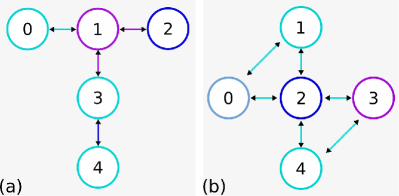
Figure 1: (Color online) Configuration of two quantum chips used in our experiments. In (a) we have the London chip, while in (b) we have the Yorktown chip configuration.

Table 1: Calibration parameters for the Yorktown chip, when used for preparing the states of Sec. IV.1.

Yorktown parameters	Q0	Q1
Frequency (GHz)	5.28	5.25
T1 ($\mu$s)	52.62	59.03
T2 ($\mu$s)	22.88	26.51
Gate error ($10^{-3}$)	1.81	1.02
Readout error ($10^{-2}$)	6.20	2.40
Multiqubit gate error ($10^{-2}$)	$\stackrel{{\scriptstyle CX0\_1}}{{4.30}}$	$\stackrel{{\scriptstyle CX1\_0}}{{4.30}}$

Table 2: Calibration parameters for the London chip, when used for preparing the one qubit ($d=2$) random quantum states of Sec. LABEL:sec:res2.

London parameters	Q0	Q1
Frequency (GHz)	5.25	5.05
T1 ($\mu$s)	46.94	63.30
T2 ($\mu$s)	76.55	50.48
Gate error ($10^{-4}$)	5.03	3.41
Readout error ($10^{-2}$)	2.50	3.50
Multiqubit gate error ($10^{-2}$)	$\stackrel{{\scriptstyle CX0\_1}}{{1.00}}$	$\stackrel{{\scriptstyle CX1\_0}}{{1.00}}$

Table 3: Calibration parameters for the Yorktown chip, when used for preparing the two qubit ($d=4$) random quantum states of Sec. LABEL:sec:res2.

Yorktown parameters	Q0	Q1	Q2
Frequency (GHz)	5.29	5.24	5.03
T1 ($\mu$s)	67.14	59.37	58.59
T2 ($\mu$s)	81.44	62.05	59.08
Gate error ($10^{-4}$)	5.56	10.11	5.83
Readout error ($10^{-2}$)	1.50	1.55	2.35
Multiqubit gate error ($10^{-2}$)	$\stackrel{{\scriptstyle CX0\_1}}{{1.57}}$	$\stackrel{{\scriptstyle CX1\_0}}{{1.57}}$	$\stackrel{{\scriptstyle CX2\_0}}{{1.55}}$
	$\stackrel{{\scriptstyle CX0\_2}}{{1.55}}$	$\stackrel{{\scriptstyle CX1\_2}}{{2.11}}$	$\stackrel{{\scriptstyle CX2\_1}}{{2.11}}$

Table 4: Average calibration parameters for the Yorktown chip, when used for preparing the three qubit ($d=8$) random quantum states of Sec. LABEL:sec:res2.

Yorktown parameters	Q0	Q1	Q2	Q3
Frequency (GHz)	5.29	5.24	5.03	5.29
T1 ($\mu$s)	66.06	58.76	52.60	52.40
T2 ($\mu$s)	26.82	26.12	74.31	36.36
Gate error ($10^{-4}$)	13.22	12.62	6.54	5.81
Readout error ($10^{-2}$)	5.52	2.87	2.38	1.33
Multiqubit gate error ($10^{-2}$)	$\stackrel{{\scriptstyle CX0\_1}}{{2.73}}$	$\stackrel{{\scriptstyle CX1\_0}}{{2.73}}$	$\stackrel{{\scriptstyle CX2\_0}}{{1.57}}$	$\stackrel{{\scriptstyle CX3\_2}}{{1.62}}$
	$\stackrel{{\scriptstyle CX0\_2}}{{1.57}}$	$\stackrel{{\scriptstyle CX1\_2}}{{2.11}}$	$\stackrel{{\scriptstyle CX2\_1}}{{2.11}}$	$\stackrel{{\scriptstyle CX2\_3}}{{1.62}}$

All qubits are always initialized in the state $|0\rangle$. After a quantum circuit is run, state tomography is performed using the function state tomography circuits(qc,qr), where $qc$ specifies the quantum circuit and $qr$ determines the qubits whose state is to be estimated. For the measurement of each observable mean value, needed for quantum state estimation, the circuit is run $8192$ times.

IV Results

In this section, we report experimental results that verify the complementarity relations presented in Sec. II. We start, in Sec. IV.1, considering a particular class of one-qubit states, what allows us to give a case study where visibility and predictability can diminish together. Afterwards, in Sec. LABEL:sec:res2, in order to report a more general verification of complementarity relations, we test them using random quantum states.

IV.1 A class of one-qubit states

As mentioned before, complementarity relations represented by Eq. (1) do not really capture a balanced exchange between $P$ and $V$, because the inequality permits that $V$ decreases due to the interaction of the system with its environment, leading to the inevitable process of decoherence, while $P$ can remain unchanged or can even decrease together with the visibility of system. For instance, we can consider the following state for a quanton

$$\rho_{A}=w\ket{\psi}_{A}\bra{\psi}+\frac{1-w}{2}I_{2\times 2},$$ (22)

where $\ket{\psi}_{A}=\sqrt{x}\ket{0}_{A}+\sqrt{1-x}\ket{1}_{A}$ with $x,w\in[0,1]$, and $I_{2\times 2}$ is the identity operator. We can consider this state of system $A$ as the result of the interaction with its own environment modeled by the depolarizing channel nielsen, which describes the situation wherein the interaction of the system with the surroundings mixes its state with the maximally entropic one. By inspecting Eq. (22), we see that when $w\to 0$ the state of system $A$ approaches a maximally incoherent state, implying that $P\to 0$ and $V\to 0$ for any predictability and visibility measures.

We can always purify $\rho_{A}$ and consider it as the result of entanglement with another system $B$, which may represent the degrees of freedom of the environment or of another auxiliary qubit. We notice that a possible purification for the state $\rho_{A}=\mathrm{Tr}_{B}|\psi\rangle_{AB}\langle\psi|$ is given as

$$\ket{\Psi}_{AB} =(-\sqrt{1-x}\ket{0}_{A}+\sqrt{x}\ket{1}_{A})\otimes\sqrt{\frac{1-w}{2}}\ket{0}_{B}$$

$$+(\sqrt{x}\ket{0}_{A}+\sqrt{1-x}\ket{1}_{A})\otimes\sqrt{\frac{1+w}{2}}\ket{1}_{B}.$$ (23)

We see that this pure state can be prepared experimentally using the following sequence of IBMQE unitary gates ibmqe:

$$\ket{\Psi}_{AB} =C_{Z}(B\to A)C_{X}(B\to A)$$

$$\hskip 14.22636ptU^{A}_{3}(\alpha,0,0)\otimes U^{B}_{3}(\theta,0,0)\ket{0,0}_{A,B}$$

$$=\Big{(}\cos\frac{\alpha}{2}\ket{0}_{A}+\sin\frac{\alpha}{2}\ket{1}_{A}\Big{)}\otimes\cos\frac{\theta}{2}\ket{0}_{B}$$

$$+\Big{(}\sin\frac{\alpha}{2}\ket{0}_{A}-\cos\frac{\alpha}{2}\ket{1}_{A}\Big{)}\otimes\sin\frac{\theta}{2}\ket{1}_{B},$$ (24)

where $U_{3}(\theta,\lambda,\phi)=\left[\begin{array}[]{cc}cos\frac{\theta}{2}&-e^{i\lambda}sen\frac{\theta}{2}\\ e^{i\phi}sen\frac{\theta}{2}&e^{i(\lambda+\phi)}cos\frac{\theta}{2}\end{array}\right]$ and $C_{Z}(B\to A)=\lx@xy@svg{\hbox{}}$