Manifold learning and nonlinear homogenization

Abstract

We describe an efficient domain decomposition-based framework for nonlinear multiscale PDE problems. The framework is inspired by manifold learning techniques and exploits the tangent spaces spanned by the nearest neighbors to compress local solution manifolds. Our framework is applied to a semilinear elliptic equation with oscillatory media and a nonlinear radiative transfer equation; in both cases, significant improvements in efficacy are observed. This new method does not rely on detailed analytical understanding of the multiscale PDEs, such as their asymptotic limits, and thus is more versatile for general multiscale problems.

65N99

1 Introduction

Homogenization is a body of theory and methods to study differential, or differential-integro equations with rapidly oscillating coefficients. It traces back to the famous work of Bensoussan-Lions-Papanicolaou [22], and builds on several other important developments [58, 39, 12, 38, 50, 17, 51, 1]. Generally speaking, the goal of homogenization is to derive asymptotic limiting equations as accurate surrogates of the original equations that do not have scale separations. The core technique is asymptotic analysis.

1.1 Goal

There are a number of famous examples that use homogenization techniques, such as elliptic equations with rapidly oscillating media [22], Schrödinger equation with small rescaled Planck constant [48], the neutron transport equation with small Knudsen number [21, 52], compressible Euler equation with small Mach number [67, 68, 83], and Boltzmann-type equations in the fluid regime [14]. All these examples have the form

(1) $$\mathcal{N}^{\epsilon}u^{\epsilon}=f\,,$$

where $\mathcal{N}^{\epsilon}$ is a partial differential operator that depends explicitly on the small parameter $\epsilon$. The term $f$ on the right-hand side represents the external information—the source terms, the boundary conditions, the initial conditions, and so on—which has no dependence on $\epsilon$. Due to the $\epsilon$-dependence of $\mathcal{N}^{\epsilon}$, the PDE is rather stiff: the solutions either exhibit high oscillations (such as the Schrödinger equation with small value of the rescaled Planck constant, or the elliptic equation with rough media), or present boundary/initial layers within which solutions change rapidly (such as the Knudsen layer in kinetic systems). The oscillations and layers themselves usually do not carry any interesting physical information; one is more interested in extracting physically meaningful quantities from the solutions directly, with these details omitted. Thus, it is important to evaluate the limiting behavior of (1) as $\epsilon\to 0$. There are two contrasting approaches in the literature that enable this task: One is analytical and the other is numerical.

The analytical approach seeks the asymptotic limit of the PDE (1), defined as follows:

(2) $$\mathcal{N}^{\ast}u^{\ast}=f\,.$$

The term “asymptotic limit” refers to the fact that for any reasonable $f$, in a certain space with a certain metric, we have

(3) $$\|u^{\epsilon}-u^{\ast}\|\to 0\quad\mbox{as $\epsilon\to 0$.}$$

A classical way to derive this limit is to perform Hilbert expansion in terms of $\epsilon$. Here, we define the ansatz

$$u^{\epsilon}=u_{0}+\epsilon u_{1}+\epsilon^{2}u_{2}+\dots$$

and substitute into (1), then balance the two sides in terms of $\epsilon$. Typically, at some level of the expansion, a closure is performed to derive the effective operator $\mathcal{N}^{\ast}$. This framework is highly effective and general; we will give explicit examples in later sections.

On the numerical side, we look for cheap solvers that compute the asymptotic limits. A typical requirement for classical numerical solvers to be accurate is that the discretization has to resolve the smallness of $\epsilon$. This can lead to high numerical and memory cost, sometimes beyond reasonable computational resources. The focus of “numerical homogenization” or “asymptotic preserving” is thus to design schemes that capture asymptotic limits of the solutions with relaxed (and thus more efficient) discretization requirements. One technique is to explore analytical results and translate them to the discrete setting: The asymptotic limiting equations are derived first, and then a “macro solver” for the limiting equation and a “micro solver” that solves the original equation, are combined in some way. This strategy has been applied to deal with the Boltzmann-type equations, the Schrödinger equation, and the elliptic equations with highly oscillatory media, under the name of designing “asymptotic preserving” schemes, finding semi-classical limits, and performing “numerical homogenization.” There is a significant drawback of this approach: The design of the numerical method is based completely on analytical understanding, so numerical development necessarily lags analytical progress. This fact significantly limits the role of multiscale computation.

This observation motivates the question that we address in this paper. Given a system of the form Eq. 1, knowing it has an asymptotic limit Eq. 2 but not knowing the specific form of this limit, can we design an efficient, accurate solver?

1.2 Approach

In this paper, we propose a numerical approach based on “compression.” Classical methods require the use of $N_{\epsilon}\sim\frac{1}{\epsilon^{\alpha}}$ grid points to achieve accuracy and stability in solving Eq. 1, for some power $\alpha>0$. Note that $N_{\epsilon}$ blows up to infinity as $\epsilon\to 0$. By contrast, the limiting equation (2) is independent of $\epsilon$, so we typically require only $N_{\ast}$ grid points (a number that is independent of $\epsilon$) to solve this system. Thus, the information carried in $N_{\epsilon}$ degrees of freedom can potentially be “compressed” into $N_{\ast}$ degrees of freedom, provided that we can tolerate an asymptotic error of order $\epsilon$ in the solution (see (3)).

How can we design an approach to solving (1) that exploits compression? Our roadmap consists three steps: (a) identify the solution set that can be compressed; (b) compress the set into a smaller effective solution set; (c) for a given new data point $f(x)$, single out the solution from the effective set. We call the first two steps the offline stage, and the last step the online stage.

For linear equations, this roadmap has been followed by several authors in [23, 27, 26, 28]. When the setup is linear, the solution set is a space, and thus information is entirely coded in representative basis functions. These basis functions can be found in the offline stage, and a Galerkin formulation can then be used to identity the linear combination of the basis for a given $f(x)$ in the online stage. To find the representative basis functions, one can utilize the random sampling technique developed for finding low rank structures of matrices in [54], where the authors proved that a few random samples are able to reconstruct the low-rank column space with high probability; see [27].

In this article, we develop the roadmap in the nonlinear setting. The extension is not straightforward. Since the solution set is not a space in the nonlinear setup, the notion of “basis function” does not even exist. Instead, we seek an $N_{\ast}$-dimensional approximating manifold in an $N_{\epsilon}$-dimensional space. For every given $f(x)$, there is a corresponding numerical solution $u^{\epsilon}$ to the original equation Eq. 1 in the $N_{\epsilon}$ space. Within $\epsilon$ distance there exists its homogenized solution $u^{\ast}$ to the limiting equation Eq. 2. Since $u^{\ast}$ relies on only $N_{\ast}$ degrees of freedom, as $f(x)$ varies, the variations of $u^{\ast}$ form a manifold of dimension at most $N_{\ast}$.

By using this argument, we formulate the homogenization problem (in the nonlinear setting) into a manifold-learning problem: Suppose we can generate a few configurations of $f(x)$ and compute the associated numerical solutions, can we learn to represent the solution manifold? Further, given a completely new configuration of $f(x)$, can we quickly identify the corresponding solution? These two questions are addressed in the offline and online stages, respectively.

Many different approaches have been proposed for manifold learning based on observed point clouds. They typically look for key features that the points share, either locally (as in local linear embedding (LLE) [82], multi-scale SVD [8, 76], local tangent space alignment [88]), or globally (as in the use of heat kernels [33, 19]). The strategy we propose here is not a direct application of any one of these ideas, but it uses elements of the the local linear embedding and multi-scale SVD approaches. Specifically, we seek local linear approximations to the solution map, and cover the solution manifold with a number of these tangent space “patches.”

We define the solution map as follows:

(4) $$\mathcal{S}^{\epsilon}:\quad f\in\mathcal{X}\to u^{\epsilon}\in\mathcal{Y}\,.$$

It maps the source term and initial/boundary conditions captured in $f(x)$ to the solution of the equation (1). To find the solution manifold, we randomly sample a large number of configurations $f_{i}$ in $\mathcal{X}$, and compute the solution $u^{\epsilon}_{i}=\mathcal{S}^{\epsilon}f_{i}\in\mathcal{Y}$ associated with each of these configurations. These solutions form a point cloud in a high dimensional space $\mathcal{Y}$. We subdivide the set of configurations $\{f_{i}\}$ into a number of small neighborhoods, and we look for the tangential approximation to the mapping (4) on each of these neighborhoods. Given a configuration $f$, we identify the neighborhood to which it belongs, and interpolate linearly to obtain the corresponding solution.

We summarize our online-offline strategy as follows. (Some modifications described in Section 2 will reduce the cost of implementation.)

• Offline: Randomly sample $f_{i}(x)$, $i=1,\dotsc,N$, and find solutions $u^{\epsilon}_{i}=\mathcal{S}^{\epsilon}f_{i}$;

• Online: Given $f(x)$:

  • Step 1: Identify the $k$-nearest neighbors of $f(x)$, call them $f_{i_{j}},j=1,2,\dotsc,k$, with $f_{i_{1}}$ being the nearest neighbor;

  • Step 2: Compute

    $$\mathcal{S}^{\epsilon}\phi\approx u^{\epsilon}_{i_{1}}+\mathsf{U}\cdot{c}\,,\quad\text{with}\quad\mathsf{U}=\begin{bmatrix}|&&|\\ u^{\epsilon}_{i_{2}}-u^{\epsilon}_{i_{1}}&\dots&u^{\epsilon}_{i_{k}}-u^{\epsilon}_{i_{1}}\\ |&&|\end{bmatrix},$$

    where $c$ is a set of coefficient that fits $f-f_{i_{1}}$ with a linear combination of $f_{i_{j}}-f_{i_{1}}$, for $j=2,3,\dotsc,k$.

In Step 2 we used the fact that the solution manifold if of low dimensional locally. To make the strategy mathematically precise, we need to address several questions, including the following.

• How should we sample $f_{i}(x)$ during the offline step?

• What metric should we use to quantify distance?

• Since computing each solution map $u^{\epsilon}_{i}=\mathcal{S}^{\epsilon}f_{i}$ is expensive, is there anyway to reduce the cost further?

We discuss these questions in the following sections. We stress that the manifold learning technique that we investigate in this paper works best when the intrinsic dimensionality of the problem is significantly smaller than the typical required degrees of freedom, and this holds true for all homogenizable problems where the discretization of the limiting equation eliminates the $\epsilon$ dependence. For problems without $\epsilon$ dependence, and the dimension of the numerical solution is only moderately large, the approach that we take is not expected to reduce cost.

1.3 The layout of the paper

We discuss the general recipe of the algorithm in Section 2, then show how the approach can be applied to two examples (a semi-linear elliptic equation and a nonlinear radiative transfer equation coupled with a temperature term) in Section 3 and Section 4, respectively. In both sections, we review the relevant homogenization theory for the equations, study the low rank structure of the tangential solution spaces, and present numerical evidence for the efficacy of our approach.

2 Framework

Our approach is a domain decomposition algorithm that makes use of Schwarz iteration.

After decomposing the domain into multiple overlapping patches, the Schwarz method solves the PDE in each patch, conditioned on agreement of solutions in the overlapping regions, which are boundary regions for the adjacent patches. At the initial step, these boundary conditions are unknown, so some initial guess is made. Subsequently, solution of PDEs on each patch alternates with updates of the solution on the overlapping regions, until convergence is obtained with respect to certain criteria. The cost of the entire process is determined by the number of iterations and the cost of the local solves, noting that, as with any domain decomposition method, the local solves can be performed in parallel. The approach is efficient when the local solves can be performed much more efficiently on the available computing resources than a solver that does not decompose the domain. The optimal domain partitioning depends on the conditioning of the problem and is often specific to the problem under study. Comprehensive descriptions of the Schwarz method appear in [84, 85].

This basic Schwarz iteration does not fully address the issue of $\epsilon$-dependence that we discussed in Section 1, since local solvers still necessarily depend on $\epsilon$. As a step toward making use of compression, we take the viewpoint that the purpose of the local solution step is to implement a boundary-to-boundary map, taking one part of the boundary conditions on a patch and using the solution of the resulting PDE to update the boundary conditions for its neighboring patches. We propose to learn the boundary-to-boundary maps in an “offline” stage, by running the local solvers as many times as are needed to attain the desired accuracy in this map. This offline stage comes with a high overhead cost, but the computation is done only once, and we hope that the cost of the online stage is greatly reduced by having the boundary-to-boundary maps available. Note that this “offline” learning process is distinct from the Offline stage discussed in Section 1. With the application of domain decomposition, it is the local behavior that needs to be learned, instead of the full $u^{\epsilon}$.

In the linear setting, building the boundary-to-boundary maps is quite straightforward. It amounts roughly to finding all discrete Green’s functions, with the degree of freedom being determined by the number of grid points on the patch boundary, with one Green’s function per grid point. In the nonlinear setting, the boundary-to-boundary map is nonlinear, so we can no longer build a linear basis, and we turn to manifold learning approach to approximate the map. Specifically, in the offline stage, we would sample randomly some configurations and find the corresponding image under the map. The resulting point cloud in high dimensional space can be viewed as samples of the manifold, which we can then learn by means of local approximate tangential planes. In the online stage, these tangential planes are used as surrogates to local boundary-to-boundary maps.

Before presenting details of the offline and online stage computations, we specify the setup and notation. We consider the following nonlinear PDE with Dirichlet boundary conditions in a domain $\Omega\subset\mathbb{R}^{2}$:

(5) $$\begin{cases}\mathcal{N}^{\epsilon}u^{\epsilon}=0\,,&\quad\text{in }\Omega\\ u^{\epsilon}=\phi,&\quad\text{on }\partial\Omega,\end{cases}$$

where, as usual, $\epsilon$ indicates the small scale of the problem. For simplicity, we will assume throughout a square geometry $\Omega=[0,L]^{2}$. The domain $\Omega$ is decomposed into overlapping rectangular patches defined by

(6) $$\Omega=\bigcup_{m\in J}\Omega_{m},\quad\text{with}\quad\Omega_{m}=(x_{m_{1}}^{(1)},x_{m_{1}}^{(2)})\times(y_{m_{2}}^{(1)},y_{m_{2}}^{(2)})\,,$$

where $m=(m_{1},m_{2})$ is a multi-index and $J$ is the collection of the indices

$$J=\{m=(m_{1},m_{2}):\,m_{1}=1,\dots,M_{1},\,m_{2}=1,\dots,M_{2}\}\,.$$

This setup is illustrated in Figure 1. For each patch we define the associated partition-of-unity function $\chi_{m}$, which has $\chi_{m}(x)\geq 0$ and

(7) $$\chi_{m}(x)=0\quad\text{on}\,\,x\in\Omega\backslash\Omega_{m}\,,\quad\sum_{m}\chi_{m}(x)=1,\quad\forall x\in\Omega\,.$$

We set $\partial\Omega_{m}$ to be the boundary of patch $\Omega_{m}$ and denote by $\mathscr{N}(m)$ the collection of indices of the neighbors of $\Omega_{m}$. In this particular 2D case, we have

(8) $$\mathscr{N}(m)=\{(m_{1}\pm 1,m_{2})\}\cup\{(m_{1},m_{2}\pm 1)\}\subset J\,.$$

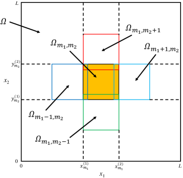
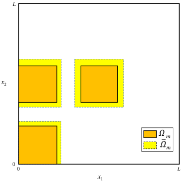
Figure 1: The plot on the left shows the domain decomposition for a square geometry. Each patch is labeled by a multi-index $m=(m_{1},m_{2})$. The adjacent patches of $\Omega_{m}$ are defined to be the patches on its north/south/west/east sides. The plot on the right demonstrates the use of local enlargement to damp boundary effects.

Assume that the equation Eq. 5 is well-posed, meaning that given $\phi$ in some function space $\mathcal{X}$, there exists a unique solution $u^{\epsilon}$ in another function space $\mathcal{Y}$. Assume further that the local nonlinear equation on patch $\Omega_{m}$ defined by

$$\begin{cases}\mathcal{N}^{\epsilon}u_{m}^{\epsilon}=0\,,&\;\text{in }\Omega_{m}\,,\\ u_{m}^{\epsilon}=\phi_{m},&\;\text{on }\partial\Omega_{m}\,,\end{cases}$$

is well-posed, given local boundary condition $\phi_{m}$ in some function space $\mathcal{X}_{m}$, and that the solution $u_{m}^{\epsilon}$ lives in space $\mathcal{Y}_{m}$. We further define the following operators.

• $\mathcal{S}^{\epsilon}_{m}$ denotes the solution operator that maps local boundary condition $\phi_{m}$ to the local solution $u_{m}^{\epsilon}$:

  $$\mathcal{S}^{\epsilon}_{m}:\mathcal{X}_{m}\to\mathcal{Y}_{m},\quad\mathcal{S}^{\epsilon}_{m}\phi_{m}=u^{\epsilon}_{m}\,.$$

• $\mathcal{I}_{m}^{l}$ denotes the trace operator for all $l\in\mathscr{N}(m)$:

  $$\mathcal{I}_{m}^{l}u_{l}^{\epsilon}=u_{l}^{\epsilon}|_{\partial\Omega_{m}\cap\Omega_{l}},\quad l\in\mathscr{N}(m)\,,$$

  which takes the value of $u^{\epsilon}_{l}$ restricted on the boundary $\partial\Omega_{m}\cap\Omega_{l}$. Here we assume that the space $\mathcal{Y}_{l}$ allows for trace.

• $\mathcal{P}_{m}$ denotes the boundary update operator, mapping $\bigoplus_{l\in\mathcal{N}(m)}\mathcal{X}_{l}$ to $\mathcal{X}_{m}$

  $$\mathcal{P}_{m}(\phi_{l},\,l\in\mathscr{N}(m))=\begin{cases}\mathcal{I}_{m}^{l}\mathcal{S}^{\epsilon}_{l}\phi_{l},&\;\text{on }\partial\Omega_{m}\cap\Omega_{l},\quad l\in\mathscr{N}(m)\,,\\ \phi|_{\partial\Omega_{m}\cap\partial\Omega},&\;\text{on }\partial\Omega_{m}\cap\partial\Omega\,.\end{cases}$$

  Note that on the points in $\partial\Omega_{m}\cap\partial\Omega$, the boundary condition from the whole domain $\Omega$ is imposed.

The offline and online stage of the algorithm are essentially to construct and to evaluate $\mathcal{P}_{m}$, as we now show.

2.1 Offline Stage

The goal of the offline stage is to construct a dictionary to approximate $\mathcal{P}_{m}$ for every $m\in J$. To eliminate any boundary layer effect, we enlarge each local patch slighly by adding a margin around its edges (except for the edges that correspond to part of the boundary of the whole domain). The enlarged domains are denoted by $\widetilde{\Omega}_{m}$ and illustrated in Figure 1.

We denote by $\widetilde{\mathcal{X}}_{m}$ the space of boundary conditions on $\partial\widetilde{\Omega}_{m}$ equipped with norm $\|\cdot\|$, and define a ball in $\widetilde{\mathcal{X}}_{m}$ as follows:

$$B(R_{m};\,\widetilde{\mathcal{X}}_{m})=\{\widetilde{\phi}\in\widetilde{\mathcal{X}}_{m}:\|\widetilde{\phi}\|\leq R_{m}\}\,.$$

First, we draw $N$ samples randomly from the ball, as follows:

$$\widetilde{\phi}_{m,i}\in B(R_{m};\,\widetilde{\mathcal{X}}_{m})\,,\quad i=1,\dots,N\,.$$

(The specific measure used in drawing depends on the particular problem being considered; we will make it more precise in the examples below.) For these samples we obtain local solutions $\widetilde{u}_{m,i}$ from the following PDEs:

(9) $$\begin{cases}\mathcal{N}^{\epsilon}\widetilde{u}_{m,i}^{\epsilon}=0\,,&\quad\text{in }\widetilde{\Omega}_{m}\\ \widetilde{u}_{m,i}^{\epsilon}=\widetilde{\phi}_{m,i}\,,&\quad\text{on }\partial\widetilde{\Omega}_{m}\end{cases}$$

We build a dictionary from these solutions by confining them in the interior $\Omega_{m}$ and the boundary $\partial\Omega_{m}$:

(10) $$\mathscr{I}_{m}=\{\psi_{m,i}=\widetilde{u}_{m,i}|_{\Omega_{m}}\}_{i=1}^{N},\quad\mathscr{B}_{m}=\{\phi_{m,i}=\widetilde{u}_{m,i}|_{\partial\Omega_{m}}\}_{i=1}^{N}\,.$$

Since the problems that we consider are homogenizable, meaning that the solution manifold is of low dimensional, the value of $N$ can be relatively small.

Remark 2.1.

Two remarks are in order.

• How to sample? That is, how to find a measure $\mu_{m}$ on $\widetilde{\mathcal{X}}_{m}$ for drawing samples? To make the setting more precise, we discretize the space $\widetilde{\mathcal{X}}_{m}$ to get $\widetilde{\mathcal{X}}^{h}_{m}$ equipped with norm $\|\cdot\|_{h}$, and define a measure $\mu_{m}^{h}$ on the ball $B(R_{m};\,\widetilde{\mathcal{X}}^{h}_{m})$. Denoting the dimension of $\widetilde{\mathcal{X}}_{m}$ by $p$, we sample the magnitude and the angle separately, that is, we take the measure as a product $\mu_{m}^{h}=\mu_{r,m}\otimes\mu_{S,m}$ with $\mu_{r,m}$ being the radial part on $(0,R_{m})$ and $\mu_{S,m}$ being the measure on the unit sphere $S^{p-1}=\{\phi\in\widetilde{\mathcal{X}}^{h}_{m}:\|\phi\|_{h}=1\}\subset\mathbb{R}^{p}$. The angular measure $\mu_{S,m}$ is chosen to be the uniform and the radial part $\mu_{r,m}$ has a density function $f(r)=\frac{D+1}{R_{m}^{D}}r^{D}$. The number $D$ here plays the role of effective dimension; it should depend on the expected dimension of solution manifold. Note that if we take $D=p-1$, the measure $\mu_{m}^{h}$ is exactly the uniform measure on the full ball $B(R_{m};\,\widetilde{\mathcal{X}}^{h}_{m})\subset\mathbb{R}^{p}$. The question of selecting $D$ in a rigorous way is left to future research. (See Appendix A and Appendix B for further details on this issue.)

• The physical boundary. To respect the boundary condition on $\partial\Omega$, the boundary patches $\Omega_{m}$ that touch the physical boundary need to be treated differently. For each sample $\widetilde{\phi}_{m,i}$, the physical boundary condition is enforced on the set $\partial\Omega_{m}\cap\partial\Omega$. Random sampling is done only on the remaining part of the patch boundary, that is, $\partial\Omega_{m}\backslash\partial\Omega$. See Appendix A and Appendix B for details.

2.2 Online Stage

The online stage finds a particular solution $u$ for given boundary data $\phi$, based on information accumulated in the offline stage. This process is carried out through a Schwarz iteration to update local boundary conditions on each patch.

Denote by $\phi^{(n)}=[\cdots\,,\phi_{m}^{(n)}\,,\cdots]$ the collection of local boundary conditions at the $n$th iteration, with $m$ being the patch index. At each iteration, we need to obtain $\phi_{m}^{(n+1)}=\mathcal{P}_{m}\phi^{(n)}$. For each $m\in J$, let $\phi_{m,i_{q}^{(n)}}$ be the $q$-th $L^{2}$-nearest neighbor of $\phi_{m}^{(n)}$ in $\mathscr{B}_{m}$, $q=1,2,\dotsc,k$. These neighbors, supported on $\partial\Omega_{m}$ lie (approximately) on a local tangential plane centered at $\phi_{m,i_{1}^{(n)}}$:

(11) $$\Phi_{m}^{(n)}=\begin{bmatrix}|&&|\\ \phi_{m,i_{2}^{(n)}}-\phi_{m,i_{1}^{(n)}}&\dots&\phi_{m,i_{k}^{(n)}}-\phi_{m,i_{1}^{(n)}}\\ |&&|\end{bmatrix}\,.$$

Associated with this plane, we also formulate the solution space centered around $\psi_{m,i_{1}^{(n)}}$:

(12) $$\Psi_{m}^{(n)}=\begin{bmatrix}|&&|\\ \psi_{m,i_{2}^{(n)}}-\psi_{m,i_{1}^{(n)}}&\dots&\psi_{m,i_{k}^{(n)}}-\psi_{m,i_{1}^{(n)}}\\ |&&|\end{bmatrix}\,.$$

Locally, the map between these two planes is approximately linear, and thus to find $\phi_{m}^{(n+1)}=\mathcal{P}_{m}\phi^{(n)}$, we look for a linear interpolation of $\phi_{m}^{(n)}$ on $\Phi_{m}^{(n)}$, and map this interpolation to $\Psi^{(n)}_{m}$. More precisely, we look for $c_{m}^{(n)}$ that solves the least-squares problem

(13) $$c_{m}^{(n)}=\operatorname*{argmin}_{v_{m}\in\mathbb{R}^{k-1}}\big{\|}\phi_{m}^{(n)}-\phi_{m,i_{1}^{(n)}}-\Phi_{m}^{(n)}v_{m}\big{\|}_{L^{2}(\partial\Omega_{m})}\,,$$

and define the approximate solution to be:

(14) $$u_{m}^{(n)}={\mathcal{S}^{\epsilon}}_{m}\phi_{m}^{(n)}\approx\psi_{m,i_{1}^{(n)}}+\Psi_{m}^{(n)}c_{m}^{(n)}\,.$$

To summarize: the map $\mathcal{P}_{m}\phi^{(n)}$ is a composition of ${\mathcal{P}}_{m}(\phi_{l}^{(n)},\,l\in\mathscr{N}(m))$ with $l\in\mathscr{N}(m)$, where

(15) $$\phi_{m}^{(n+1)}={\mathcal{P}}_{m}(\phi_{l}^{(n)},\,l\in\mathscr{N}(m))=\mathcal{I}_{m}^{l}{\mathcal{S}^{\epsilon}}_{l}\phi_{l},\quad\text{on }\partial\Omega_{m}\cap\Omega_{l}\,.$$

Once a preset error tolerance is achieved, at some step $n$ (usually because the local boundary condition barely changes), the global solution is patched up as follows:

(16) $$u^{(n)}=\sum_{m\in J}\chi_{m}u_{m}^{(n)}\,,$$

where $u_{m}^{(n)}$ is the local solution Eq. 14 and $\chi_{m}:\Omega\rightarrow\mathbb{R}$ is the smooth partition of unity associated with the partition.

We summarize the procedure in Algorithm 1.

Remark 2.2.

The Johnson-Lindenstrauss lemma [65] indicates that the search for $d$-dimensional $k$ nearest neighbors in a data set of size $N$, with distance error $\delta$, can be done in query time $O\Bigl{(}kd\frac{\log N}{\delta^{2}}\Bigr{)}$ and storage cost $N^{O(\log(1/\delta)/\delta^{2})}+O\Bigl{(}d\bigl{(}N+\frac{\log N}{\delta^{2}}\bigr{)}\Bigr{)}$ [62, 11]. In addition, a cost of $O(k^{2}d)$ is incurred at each iteration, due to $L^{2}$ minimization for each patch via QR factorization. In our setting, $d$ is equal to the degrees of freedom on the boundary $\partial\Omega_{m}$.

Remark 2.3.

To avoid notational complexity, the discussion above does not consider the physical boundary $\partial\Omega$. If a patch contains part of $\partial\Omega$, then that particular section of the patch is not updated. The true boundary condition $\phi$ is enforced in every iteration. The derivation is straightforward and is omitted from the discussion.

Algorithm 1 Multiscale solver for nonlinear homogenizable equations Eq. 5.

1:Given the radius $R_{m}$, the number of nearest neighbors $k$, the tolerance $\delta$ and the initial guess of boundary conditions $\phi_{m}^{(0)}$ on each patch $m\in J$.

2:Domain Decomposition:

3:      Decompose $\Omega$ into overlapping patches: $\Omega=\bigcup_{m\in J}\Omega_{m}$, and enlarge each patch to obtain $\widetilde{\Omega}_{m}$.

4:Offline Stage: Prepare local dictionaries on interior patches $\Omega_{m}$.

5:     Step 1: For each $m\in J_{i}$, generate $N$ samples $\widetilde{\phi}_{m,i}$ from $B(R_{m};\widetilde{\mathcal{X}}_{m})$;

6:     Step 2: For all $i$, call function

$$\widetilde{u}_{m,i}=\text{LocPDESol}(\widetilde{\Omega}_{m},\widetilde{\phi}_{m,i})\,;$$

7:     Step 3: Collect local dictionaries according to Eq. 10 for $\mathscr{B}_{m}$ and $\mathscr{I}_{m}$.

8:Online Stage: Schwarz iteration.

9:     while $\sum_{m}\|\phi_{m}^{(n)}-\phi_{m}^{(n-1)}\|_{L^{2}(\partial\Omega_{m})}\geq\delta$ do

10:         for $m\in J$ do

11:              Search for $k$-nearest neighbors of $\phi_{m}^{(n)}$ in $\mathscr{B}_{m}$;

12:              Solve $c_{m}^{(n)}$ from the least-squares problem Eq. 13;

13:              Update $\phi_{m}^{(n+1)}$ by Eq. 15.

14:         end for

15:         $n\leftarrow n+1$

16:     end while

17:return Global solution $u^{(n)}$ defined by Eq. 16.

1:function LocPDESol(Local domain $\Omega_{m}$, Boundary condition $\phi_{m}$)

2:     Perform the standard finite difference or finite element methods to solve the local nonlinear equation Eq. 9;

3:return Local solution $u_{m}$

4:end function

3 Example 1: Semilinear elliptic equations with highly oscillatory media

In this section, we apply the methodology described above to solve semilinear elliptic equations. Semilinear elliptic equations with multiscale structures arise in a variety of situations, for instance, in nonlinear diffusion generated by nonlinear sources [66], and in the gravitational equilibrium of stars [75, 24]. As fundamental models in many areas of physics and engineering, the equations have received considerable attention.

We consider the equation

(17) $$\begin{cases}-\nabla_{x}\cdot\left(A\left(x,\tfrac{x}{\epsilon}\right)\nabla_{x}u^{\epsilon}\right)+f(u^{\epsilon})=0,\quad&x\in\Omega\,,\\ u^{\epsilon}(x)=\phi(x),\quad&x\in\partial\Omega\,.\end{cases}$$

The physical domain is $\Omega\subset\mathbb{R}^{d}$ with $d\geq 1$, and Dirichlet boundary condition is given as $\phi(x)$. The permeability $A(x,y)=(a_{ij}(x,y))_{d\times d}:\Omega\times\mathbb{R}^{d}\to\mathbb{R}^{d\times d}$ depends on both the slow variable $x$ and the fast variable $y=x/\epsilon$ and is highly oscillatory. The function $f:\mathbb{R}\rightarrow\mathbb{R}$ describes the nonlinear source term. The solution $u^{\epsilon}$ presents one component in a chemical reaction or one species of a biological system.

The well-posedness of equation Eq. 17 is classical. We assume that the permeability $A$ is a symmetric matrix with $L^{\infty}$-coefficients satisfying the standard coercivity condition, and that the nonlinear function $f$ is locally Lipschitz continuous and increasing. Then, assuming the boundary $\partial\Omega$ is smooth enough, given boundary condition $\phi\in H^{1/2}(\partial\Omega)\cap L^{\infty}(\partial\Omega)$, the problem Eq. 17 has a unique $H^{1}$-solution satisfying the maximum principle. We refer to [49, 30] for details.

3.1 Homogenization limit

The semilinear elliptic equation Eq. 17 has a homogenization limit as $\epsilon\rightarrow 0$. Supposing that $A(x,y)$ is smooth and periodic in $y$ with period $I=[0,1]^{d}$, then as $\epsilon\rightarrow 0$, the solution $u^{\epsilon}$ converges to a limit $u^{\ast}$ that satisfies the same class of semilinear elliptic equations with an $\epsilon$-independent effective permeability $A^{\ast}(x)=(a_{ij}^{\ast}(x))_{d\times d}$:

(18) $$\begin{cases}-\nabla_{x}\cdot(A^{\ast}(x)\nabla_{x}u^{\ast})+f(u^{\ast})=0,\quad&x\in\Omega\,,\\ u^{\ast}(x)=\phi(x),\quad&x\in\partial\Omega\,.\end{cases}$$

This equation (in particular, the effective permeability $A^{\ast}(x)$) can be derived by expanding the equation Eq. 17 into different orders of $\epsilon$. Rigorous proofs are given in [22, 20, 80]. We cite the following theorem as a reference:

Theorem 3.1 (Section 16.3 in Chapter 1 of [22]; see also [7]).

Assume the boundary $\partial\Omega$ is smooth. Given $\phi(x)\in H^{1/2}(\partial\Omega)\cap L^{\infty}(\partial\Omega)$, let $u^{\epsilon}$ be the unique solution to the semilinear elliptic equation Eq. 17 in $H^{1}(\Omega)\cap L^{\infty}(\Omega)$. Assume that the permeability $A(x,y)$ is periodic in $y$ with period $I=[0,1]^{d}$ and that $A(x,\cdot)\in C^{1}(I)$. Then the solution $u^{\epsilon}$ converges weakly in $H^{1}(\Omega)$ as $\epsilon\rightarrow 0$ to $u^{\ast}$ (the solution to Eq. 18), where the permeability $A^{\ast}(x)=(a_{ij}^{\ast}(x))_{d\times d}$ is defined by

(19) $$a_{ij}^{\ast}(x)=\int_{I}\sum_{k,l}a_{kl}(x,y)(\delta_{ki}+\partial_{y_{k}}\chi_{i})(\delta_{lj}+\partial_{y_{l}}\chi_{j})\mathrm{d}y\,.$$

Here, for each fixed coordinate $j=1,2,\dotsc,d$, the function $\chi_{j}(x,y)$ is the solution of the following cell problem with periodic boundary condition on $I$:

(20) $$\nabla_{y}\cdot(A(x,y)\nabla_{y}(\chi_{j}(x,y)+y_{j}))=0\,.$$

To solve Eq. 17, the discretization has to resolve $\epsilon$, but in the limit Eq. 18, the discretization is independent of $\epsilon$. This suggests significant opportunities for cost savings: The information contained in $O(1/\epsilon)$ degrees of freedom can be expressed with $O(1)$ degrees of freedom.

The literature for numerical homogenization is rich, particularly for the linear setting when $f=0$. Relevant approaches include the multiscale finite element method (MsFEM) [58, 44, 59], the heterogeneous multiscale method (HMM) [39, 4, 40], the generalized finite element method [13, 12], upscaling based on harmonic coordinates [79], elliptic solvers based on $\mathcal{H}$-matrices [18, 53], the reduced basis method [3, 2], the use of localization [77], and the methods based on random SVD [27, 26, 28], to name a few. The analytical understanding of the homogenized equation is essential in the construction of these methods [7]. When randomness presents, one can also look for low dimensional representation of the solutions in the random space [56, 74, 57, 32].

The literature for nonlinear problems is not as rich. There are several works on quasilinear problems, all of which can be seen as extensions of classical methods, including the MsFEM [43, 29, 42], the HMM [40, 5], the generalized finite element method [41], the local orthogonal decomposition method [55], the reduced basis method [3] and nonlocal multicontinua upscaling [31]. These solvers must be designed carefully for specific nonlinear equations. By contrast, our method makes use of the low-rankness of the solution sets and could be applied with minor modification to different equations.

3.2 Low dimensionality of the tangent space

We now study the structure of the tangent space of the solution manifold, verifying in particular the low dimension assumption. We choose some point $\overline{u}^{\epsilon}$ on the solution manifold and then randomly pick a neighboring solution point $u^{\epsilon}$. These two points are solutions to Eq. 17 computed from distinct nearby boundary configurations $\overline{\phi}$ and $\phi$, that is,

(21) $$\overline{u}^{\epsilon}|_{\partial\Omega}=\overline{\phi}\,,\quad u^{\epsilon}|_{\partial\Omega}=\phi\,,\quad\text{with}\quad\|\overline{\phi}-\phi\|_{L^{\infty}(\partial\Omega)}=\mathcal{O}(\delta)\,.$$

By varying $\phi$ around $\overline{\phi}$, one can build a small point cloud around $\overline{u}^{\epsilon}$. Denoting $\delta u^{\epsilon}:=u^{\epsilon}-\overline{u}^{\epsilon}$, we have immediately that

(22) $$\begin{cases}-\nabla_{x}\cdot\left(A\left(x,\tfrac{x}{\epsilon}\right)\nabla_{x}\delta u^{\epsilon}\right)+f(\overline{u}^{\epsilon}+\delta u^{\epsilon})-f(\overline{u}^{\epsilon})=0,\quad&x\in\Omega\,,\\ \delta u^{\epsilon}(x)=\phi(x)-\overline{\phi}(x),\quad&x\in\partial\Omega\,.\end{cases}$$

In the small-$\delta$ regime, this collection of solution differences $\delta u^{\epsilon}$ spans the tangent plane. We claim this tangent plane is low dimensional, so that it inherits the homogenization effect of the original equation. We have the following result.

Theorem 3.2.

Let $\delta u^{\epsilon}$ solve Eq. 22. Assume $A(x,y)=(a_{ij}(x,y))_{d\times d}$ is periodic in $y$ with period $I=[0,1]^{d}$. The equation has homogenization limit when $\epsilon\to 0$, meaning there exists a limiting permeability $A^{\ast}(x)=(a_{ij}^{\ast}(x))_{d\times d}$, determined by $A(x,y)$ via equation Eq. 19 and Eq. 20, so that $\delta u^{\epsilon}\to\delta u^{\ast}$ and $\delta u^{\ast}$ solves:

(23) $$\begin{cases}-\nabla_{x}\cdot(A^{\ast}(x)\nabla_{x}\delta u^{\ast})+f(\overline{u}^{\ast}+\delta u^{\ast})-f(\overline{u}^{\ast})=0,\quad&x\in\Omega\,,\\ \delta u^{\ast}(x)=\phi(x)-\overline{\phi}(x),\quad&x\in\partial\Omega\,,\end{cases}$$

where $\overline{u}^{\ast}$ solves:

(24) $$\begin{cases}-\nabla_{x}\cdot(A^{\ast}(x)\nabla_{x}\overline{u}^{\ast})+f(\overline{u}^{\ast})=0,\quad&x\in\Omega\,,\\ u^{\ast}(x)=\overline{\phi}(x),\quad&x\in\partial\Omega\,.\end{cases}$$

Further, for small $\delta$, equation Eq. 23, in the leading order of $\delta$, becomes:

(25) $$-\nabla_{x}\cdot(A^{\ast}(x)\nabla_{x}\delta u^{\ast})+f^{\prime}(\overline{u}^{\ast}(x))\delta u^{\ast}=0\,.$$

Proof 3.3.

By applying Theorem 3.1 to the equation for $\overline{u}^{\epsilon}$, which is

$$\begin{cases}-\nabla_{x}\cdot\left(A\left(x,\tfrac{x}{\epsilon}\right)\nabla_{x}\delta\overline{u}^{\epsilon}\right)+f(\overline{u}^{\epsilon})=0,\quad&x\in\Omega\,,\\ \delta\overline{u}^{\epsilon}(x)=\overline{\phi}(x),\quad&x\in\partial\Omega\,,\end{cases}$$

we have by comparing with equation Eq. 17 for $u^{\epsilon}$ that $\overline{u}^{\epsilon}$ converges weakly to $\overline{u}^{\ast}$, which solves Eq. 24, and that $u^{\epsilon}$ converges weakly to $u^{\ast}$, which solves Eq. 18. From the definition $\delta u^{\epsilon}=u^{\epsilon}-\overline{u}^{\epsilon}$, we find that $\delta u^{\epsilon}$ converges to $\delta u^{\ast}$, which solves Eq. 23.

This theorem suggests that for the discretized equation, because of the existence of the homogenized limit, the tangent plane of the discrete solution is approximately low-rank. The space spanned by $\{\delta u^{\epsilon}\}$ can be approximately spanned by $\{\delta u^{\ast}\}$, which solves the limiting equation Eq. 23 without dependence on small scales.

3.3 Implementation

We apply Algorithm 1 to equation (17) with $f(u)=u^{3}$ and $\Omega=[0,L]^{2}\subset\mathbb{R}^{2}$, that is,

(26) $$\begin{cases}-\nabla_{x}\cdot\left(a\left(x,\tfrac{x}{\epsilon}\right)\nabla_{x}u\right)+u^{3}=0\,,\quad&x\in\Omega=[0,L]^{2},\\ u(x)=\phi(x),\quad&x\in\partial\Omega.\end{cases}$$

We use the domain decomposition strategy of Section 2 to solve this system. Since $\Omega$ is convex and the coefficient $a(x,x/\epsilon)$ belongs to $L^{\infty}(\Omega)$, we can show using the monotone method [9, 30] that the equation is well-posed, having a unique solution if we set

$$\mathcal{X}=H^{1/2}(\partial\Omega)\cap L^{\infty}(\partial\Omega),\quad\mathcal{Y}=H^{1}(\Omega)\cap L^{\infty}(\Omega)\,.$$

In the offline stage, we generate $N$ samples for each enlarged patch $\widetilde{\Omega}_{m}$, as follows:

$$\widetilde{\phi}_{m,i}\in B(R_{m};\,\widetilde{\mathcal{X}}_{m})\,,\quad i=1,\dots,N\,.$$

(The measure we use for sampling is discussed in Appendix A.) We equip the ball with $H^{1/2}$-norm:

(27) $$B(R_{m};\,\widetilde{\mathcal{X}}_{m})=\{\widetilde{\phi}\in\widetilde{\mathcal{X}}_{m}:\|\widetilde{\phi}\|_{H^{1/2}(\partial\Omega_{m})}\leq R_{m}\}\,.$$

We compute the $H^{1/2}(\partial\Omega)$-norm numerically using the Gagliardo seminorm [35]:

$$\|\phi\|_{H^{1/2}(\partial\Omega)}=\sqrt{\int_{\partial\Omega}|\phi(x)|^{2}\mathrm{d}x+\iint_{\partial\Omega\times\partial\Omega}\frac{|\phi(x)-\phi(y)|^{2}}{|x-y|^{2}}\mathrm{d}x\mathrm{d}y}\,.$$

For these boundary configurations, we solve the equation

(28) $$\begin{cases}-\nabla_{x}\cdot\left(a\left(x,\tfrac{x}{\epsilon}\right)\nabla_{x}\widetilde{u}_{m,i}\right)+\widetilde{u}_{m,i}^{3}=0\,,&\quad x\in\widetilde{\Omega}_{m}\,,\\ \widetilde{u}_{m,i}(x)=\widetilde{\phi}_{m,i}(x)\,,&\quad x\in\partial\widetilde{\Omega}_{m}\,,\end{cases}$$

and build two sets of dictionaries by confining the solutions in the interior $\Omega_{m}$ and the boundary $\partial\Omega_{m}$, as follows:

(29) $$\mathscr{I}_{m}=\{\psi_{m,i}=\widetilde{u}_{m,i}|_{\Omega_{m}}\}_{i=1}^{N},\quad\mathscr{B}_{m}=\{\phi_{m,i}=\widetilde{u}_{m,i}|_{\partial\Omega_{m}}\}_{i=1}^{N}\,.$$

In the online stage, local boundary conditions are updated according to Eq. 14 at each iteration, with coefficients computed from Eq. 13. The local tangent space is found by searching for the $k$ nearest neighbors in the dictionary $\mathscr{B}_{m}$, mapped to the dictionary $\mathscr{I}_{m}$ (see (29)). We use the $L^{2}$ norm to measure the distance between the newly generated solutions and the older solution set.

Once a preset error tolerance is achieved (at step $n$, say), the global solution is patched up from the local pieces, as follows:

(30) $$u^{(n)}=\sum_{m\in J}\chi_{m}u_{m}^{(n)}\,,$$

where $u_{m}^{(n)}$ is the local solution on $\Omega_{m}$ at the $n$-th step and $\chi_{m}:\Omega\rightarrow\mathbb{R}$ is a smooth partition of unity.

3.4 Numerical Tests

We present numerical results for (26) in this subsection. We use $L=1$, yielding the domain $\Omega=[0,1]^{2}$, and define the oscillatory media as follows:

$$a(x,y,x/\epsilon,y/\epsilon)=2+\sin(2\pi x)\cos(2\pi y)+\frac{2+1.8\sin(2\pi x/\epsilon)}{2+1.8\cos(2\pi y/\epsilon)}+\frac{2+\sin(2\pi y/\epsilon)}{2+1.8\cos(2\pi x/\epsilon)}\,.$$

The boundary condition is

$$\phi(x,0) =-\sin(2\pi x)\,,\quad \phi(x,1) =\sin(2\pi x)\,,$$

$$\phi(0,y) =\sin(2\pi y)\,,\quad \phi(1,y) =-\sin(2\pi y)\,.$$

To form the partitioning, the whole domain $\Omega$ is divided equally into $4\times 4$ non-overlapping squares, and then each square is enlarged by $\Delta x_{\text{o}}=.0625$ on the sides that do not intersect with $\partial\Omega$, to create overlap. We thus have $M_{1}=M_{2}=4$, with $\Omega_{m}$ for $m=(m_{1},m_{2})$, $m_{1}=1,2,3,4$ and $m_{2}=1,2,3,4$, defined by

$$\Omega_{m} =\left[\max\left(\tfrac{m_{1}-1}{M_{1}}-\Delta x_{\text{o}},0\right),\min\left(\tfrac{m_{1}}{M_{1}}+\Delta x_{\text{o}},1\right)\right]$$

$$\quad\times\left[\max\left(\tfrac{m_{2}-1}{M_{2}}-\Delta x_{\text{o}},0\right),\min\left(\tfrac{m_{2}}{M_{2}}+\Delta x_{\text{o}},1\right)\right]\,,\quad m=(m_{1},m_{2})\in J\,.$$

Denote $\Omega_{m}=[x_{m}^{(1)},x_{m}^{(2)}]\times[y_{m}^{(1)},y_{m}^{(2)}]$. The partition of unity function $\chi_{m}$ is defined by normalizing the bump functions on the overlapping domains. More precisely, we first define a bump function $f_{m}:\Omega\to\mathbb{R}$ supported on $\Omega_{m}$ as follows:

$$f_{m}(x,y)=\begin{cases}\exp\left(-\frac{1}{1-|x-x_{m}|/\alpha_{m}}-\frac{1}{1-|y-y_{m}|/\beta_{m}}\right)\,,\quad(x,y)\in\Omega_{m}\\ 0\,,\quad\text{Otherwise}\end{cases}\,,$$

where $x_{m}=\frac{x_{m}^{(2)}-x_{m}^{(1)}}{2}$, $y_{m}=\frac{y_{m}^{(2)}-y_{m}^{(1)}}{2}$, $\alpha_{m}=\frac{x_{m}^{(1)}+x_{m}^{(2)}}{2}$ and $\beta_{m}=\frac{y_{m}^{(1)}+y_{m}^{(2)}}{2}$. The partition of unity $\chi_{m}:\Omega\to\mathbb{R}$ is then obtained by

$$\chi_{m}(x,y)=\frac{f_{m}(x,y)}{\sum_{m\in J}f_{m}(x,y)}\,.$$

A standard finite-volume scheme with uniform grid is used for discretization, the corresponding nonlinear discrete system being solved by Newton’s method. The reference solutions are computed on the fine mesh with $h=2^{-12}=\tfrac{1}{4096}$. Unless otherwise specified, other computations are performed with mesh size $h=2^{-9}=\tfrac{1}{512}$. Denoting the numerical solution by $u_{ij}\approx u(x_{i},y_{j})$, we use the classical discrete $L^{2}$ norm

$$\|u\|_{L^{2}}=h\sqrt{\sum_{i,j=0}^{p}|u_{ij}|^{2}}\,,$$

and the energy norm

$$\|u\|_{\mathcal{E}}=h\sqrt{\sum_{j=0}^{p}\sum_{i=0}^{p-1}a_{i+1/2,j}\left|\frac{u_{i+1,j}-u_{ij}}{h}\right|^{2}+\sum_{i=0}^{p}\sum_{j=0}^{p-1}a_{i,j+1/2}\left|\frac{u_{i,j+1}-u_{ij}}{h}\right|^{2}}\,,$$

and define the relative errors accordingly by

$$\mbox{\rm relative $L^{2}$ error}=\frac{\|u_{\text{ref}}-u_{\text{approx}}\|_{L^{2}}}{\|u_{\text{ref}}\|_{L^{2}}}\,,\quad\mbox{\rm relative energy error}=\frac{\|u_{\text{ref}}-u_{\text{approx}}\|_{\mathcal{E}}}{\|u_{\text{ref}}\|_{\mathcal{E}}}.$$

We first describe numerical experience with the offline stage. Each interior patch $\Omega_{m}$ is enlarged by a margin $\Delta x_{\text{b}}$ to damp the boundary effects. The resulting buffered patch $\widetilde{\Omega}_{m}$ is concentric with $\Omega_{m}$; see Figure 2. In the plots shown below, we study the patch indexed by $m=(2,2)$.

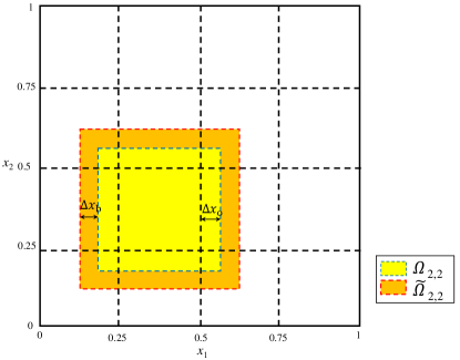
Figure 2: Buffered domain decomposition.

To build the local dictionary, we generate $64$ samples randomly in $B(R_{2,2},\widetilde{X}_{2,2})$, where $R_{2,2}=20$. (The sampling scheme is discussed in Appendix A.) We compute the local solutions with these boundary conditions on $\widetilde{\Omega}_{2,2}$, for several choices of buffer size $\Delta x_{\text{b}}$, and subtract the solutions from the reference solution, confined to $\Omega_{2,2}$. This procedure forms the tangent space centered around the reference solution in this particular patch. In Figure 3a we plot the singular value decay of this tangent space, for $\epsilon=2^{-4}$. It is clear that the singular values decay exponentially, with a larger buffer margin $\Delta x_{\text{b}}$ leading to a faster decay rate. This observation suggests that the tangent space is approximately low dimensional. We then project the reference solution onto the space spanned by its closest neighbors. As the number of neighbors increases, the relative error decays exponentially, as seen in Fig. 3b. When the buffer margin is $\Delta x_{\text{b}}=2^{-4}$, we achieve $99\%$ accuracy with $30$ neighbors. By comparison, the degrees of freedom for this patch is determined by the total number of grid points on the boundary of this patch — 768, in this particular case.

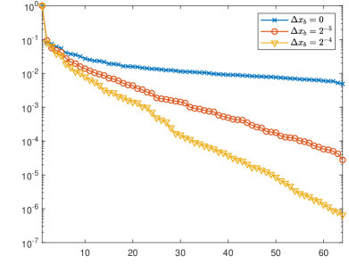
(a)

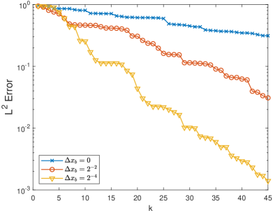
(b)

Figure 3: (a) The singular value decay of the tangent space (centered around the reference solution) on patch $\Omega_{2,2}$, for different values of the buffer margin $\Delta x_{\text{b}}$. (b) The relative error of the projection of reference solution onto the space spanned by the nearest $k$ neighbors on $\Omega_{2,2}$. The distance is measured in $L^{2}(\Omega_{2,2})$. $\epsilon=2^{-4}$ in both plots.

In the online stage, we set the stopping criterion to be

$$\sum_{m}\|\phi_{m}^{(n)}-\phi_{m}^{(n-1)}\|_{L^{2}(\partial\Omega_{m})}<10^{-5}\,,$$

where the upper index $(n)$ indicates the evaluation of the solution in the $n$-th iteration on $\mathcal{X}_{m}$, which is the boundary of $\Omega_{m}$. The initial guess for all local boundary condition is chosen (trivially) to be $\phi_{m}^{(0)}|_{\partial\Omega_{m}\backslash\partial\Omega}=0$ and $\phi_{m}^{(0)}|_{\partial\Omega_{m}\cap\partial\Omega}=\phi|_{\partial\Omega_{m}\cap\partial\Omega}$.

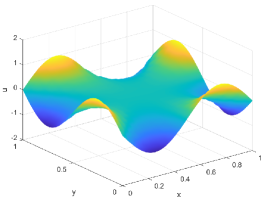
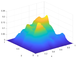
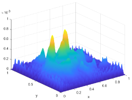
Figure 4: Computed solutions. Left panel shows the reference solution obtained with fine grids of width $h=2^{-12}$. Middle and right panels show the numerical error $|u-u_{\text{ref}}|$ obtained with $k=5$ and $k=30$, respectively.

In Figure 4, we compare the numerical solutions using the space spanned by $k=5$ and $k=40$ nearest neighbors. The buffer margin is $\Delta x_{\text{b}}=2^{-4}$, and we set $\epsilon=2^{-4}$. We also document the error behavior as a function of $k$, $\epsilon$, and $\Delta x_{\text{b}}$. In Figure 5, we plot the error decay as a function of $k$ (the number of neighbors used in the online stage) for different values of $\epsilon$ and $\Delta x_{\text{b}}$. The decay is independent of $\epsilon$, indicating the rank structure is not influenced by small scales in the equation. As the number of neighbors $k$ increases, the global relative $L^{2}$ and energy error decays exponentially provided a buffer zone is present. When $\Delta x_{\text{b}}=0$ (no buffer), the boundary layer effect is strong, and convergence is not obtained, meaning that the local solution cannot be well approximated from the dictionary.

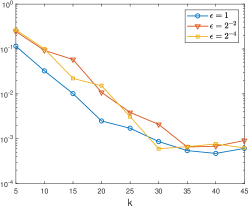
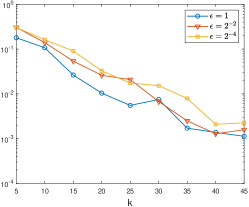
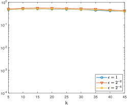
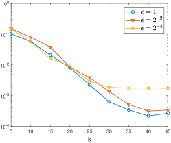
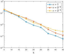
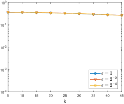
Figure 5: The top row of plots shows the global $L^{2}$ error as a function of $k$ with different $\epsilon$ and buffer zone size $\Delta x_{\text{b}}$. The bottom row of plots shows the global energy error. The three columns of plots represent $\Delta x_{\text{b}}=2^{-4},2^{-5},0$, respectively.

We show CPU times in Table 1, comparing the reduced model for different values of $k$ with the classical Schwarz iteration, for $\epsilon=2^{-4}$ and $\Delta x_{\text{b}}=2^{-4}$. The same stopping criterion is used for all variants. The online stage of each reduced model is significantly faster than the classical Schwarz iteration. Even with $k=40$ neighbors involved in the local solution reconstruction, our method requires $1.12$s, compared to $187.8$s required by the classical Schwarz method. While the offline preparation is expensive in general, it is still cheaper in this example than the classical Schwarz iteration for solving a single problem. Because the dictionary can be reused, our method has a strong advantage in situations where many solutions corresponding to different boundary conditions are needed. This is a typical situation in inverse problems, where to determine the unknown media, many boundary configurations are imposed and numerical solutions are computed to compare with measurements [25].

	CPU Time (s) ($\epsilon=2^{-4}$)
	offline	online
Reduced model $k=5$	135.6914	0.173712
Reduced model $k=10$		0.305707
Reduced model $k=20$		0.462857
Reduced model $k=30$		0.696785
Reduced model $k=40$		1.124082
Classical Schwarz	—	187.7705

Table 1: CPU time comparison between our reduced method with $k=5,10,20,30,40$ and classical Schwarz method.

4 Example 2: Nonlinear radiative transfer equation

Here we study the application of Algorithm 1 to a nonlinear radiative transfer equation. Radiative transfer is the physical phenomenon of energy transfer in the form of electromagnetic radiation, and the radiative transfer equations describe the absorption or scattering of radiation as it propagates through a medium. The equations are important in optics, astrophysics, atmospheric science, remote sensing [78], and other applications.

We denote by $I^{\epsilon}(x,v)$ the distribution function of photon particles at location $x$ moving with velocity $v$ in the physical domain $\mathcal{D}\subset\mathbb{R}^{3}$ and the velocity domain $\mathcal{V}=\mathbb{S}^{2}$. Also denote by $T^{\epsilon}(x)$ the temperature profile across domain $\mathcal{D}$. We consider a nonlinear system of equations that couples the photon particle distribution with the temperature profile. The steady state equations are

(31) $$\begin{cases}\epsilon v\cdot\nabla_{x}I^{\epsilon}=B(T^{\epsilon})-I^{\epsilon},\;\;\text{for }(x,v)\in\mathcal{K}=\mathcal{D}\times\mathcal{V},\\ \epsilon^{2}\Delta_{x}T^{\epsilon}=B(T^{\epsilon})-\langle I^{\epsilon}\rangle,\;\;\text{for }x\in\mathcal{D}\,,\end{cases}$$

with the velocity-averaged intensity given by

(32) $$\langle I\rangle(x)=\int_{\mathcal{V}}I(x,v)\mathrm{d}\mu(v)\,.$$

Here, $\mu(v)$ is a normalized uniform measure on $\mathcal{V}$ and $B(T)$ is a nonlinear function of $T$, typically defined as

(33) $$B(T)=\sigma T^{4},$$

where $\sigma$ is a scattering coefficient [70, 86]. The parameter $\epsilon$ is called the Knudsen number, standing for the ratio of the mean free path and the typical domain length. When the medium is highly scattering and optically thick, the mean free path is small, with $\epsilon\ll 1$. The scattering coefficient $\sigma$ is independent of $\epsilon$.

We consider a slab geometry. Assuming the $y$ and $z$ directions to be homogeneous, then since $v=(\cos\theta,\sin\theta\sin\varphi,\sin\theta\cos\varphi)$, the $v_{x}$ component becomes $\cos\theta\in[-1,1]$. The problem is simplified to:

(34) $$\begin{cases}\epsilon v\partial_{x}I^{\epsilon}=B(T^{\epsilon})-I^{\epsilon}\\ \epsilon^{2}\partial_{x}^{2}T^{\epsilon}=B(T^{\epsilon})-\langle I^{\epsilon}\rangle\end{cases},\quad(x,v)\in\mathcal{K}=[a,b]\times[-1,1]\,,$$

with $\langle I\rangle(x)=\frac{1}{2}\int_{-1}^{1}I(x,v)\mathrm{d}v$.

We provide incoming boundary conditions that specify the distribution of photons entering the domain. The boundary condition itself has no $\epsilon$ dependence; we have

(35) $$I^{\epsilon}(x,v)=I_{b}(x,v)\;\;\text{ on }\Gamma_{-}\,,\quad T^{\epsilon}(x)=T_{b}(x)\;\;\text{ on }\partial\mathcal{D}\,.$$

Here $\Gamma_{\pm}$ collect the coordinates at the boundary with velocity pointing into or out of the domain:

$$\Gamma_{\pm}=\{(x,v):x\in\partial\mathcal{D}\,,\pm v\cdot n_{x}>0\}\,,$$

and $n_{x}$ denotes the unit outer normal vector at $x\in\partial\Omega$.

4.1 Homogenization limit

The equations Eq. 31 have a homogenization limit. As $\epsilon\to 0$, the right hand side of the equations dominates, and by balancing the scales we obtain

$$I^{\epsilon}\sim\langle I^{\epsilon}\rangle\sim\sigma(T^{\epsilon})^{4}\sim I^{\ast}\sim\sigma(T^{\ast})^{4}\,.$$

To find the equation satisfied by $T^{\ast}$, we expand the equations Eq. 31 up to second order in $\epsilon$. Rigorous results are shown in [72, 69, 15, 16]. We cite the following theorem captures the results needed here.

Theorem 4.1 (Modification of Theorem 3.2 in [69]).

Let $\mathcal{D}\subset\mathbb{R}^{3}$ be bounded and $\partial\mathcal{D}$ be smooth. Assuming that the boundary conditions Eq. 35 are positive and that $T_{b}\in H^{1/2}(\partial\mathcal{D})\cap L^{\infty}(\partial\mathcal{D})$ and $I_{b}\in L^{\infty}(\Gamma_{-})$, then the nonlinear radiative transfer equation Eq. 31 has a unique positive solution $(I^{\epsilon},T^{\epsilon})\in L^{\infty}(\mathcal{K})\times L^{\infty}(\mathcal{D})$. If we assume further that $(I_{b},T_{b})\geq\gamma>0$ and $I_{b}=B(T_{b})$ a.e. on $\Gamma_{-}$, then the solution in the limit as $\epsilon\rightarrow 0$ converges weakly to $(B(T^{\ast}),T^{\ast})$, where the limiting temperature $T^{\ast}$ is the unique positive solution to the following PDE:

(36) $$\Delta_{x}(T^{\ast}+B(T^{\ast})/3)=0\,,\quad\text{for}\quad x\in\mathcal{D}\,,$$

equipped with Dirichlet boundary data $T^{\ast}|_{\partial\mathcal{D}}=T_{b}$. The convergence of $T^{\epsilon}$ is in $H^{1}(\mathcal{D})$ weak and the convergence of $I^{\epsilon}$ is in $L^{\infty}(\mathcal{K})$ weak-$\ast$.

Remark 4.2.

Without appropriate boundary conditions $I_{b}=B(T_{b})$, boundary layers of width $O(\epsilon)$ may emerge as $\epsilon\to 0$. It is conjectured in [69] that the boundary layers in the neighborhood of each point $\hat{x}\in\partial\mathcal{D}$ can be characterized by the following one-dimensional Milne problem for $y\in[0,\infty)$:

$$-(v\cdot n_{\hat{x}})\partial_{y}\hat{I} =B(\hat{T})-\hat{I}\,,$$

$$\partial_{y}^{2}\hat{T} =B(\hat{T})-\langle\hat{I}\rangle\,,$$

$$\hat{T}(0) =T_{b}(\hat{x}),\quad\hat{I}(0,v)=I_{b}(\hat{x},v),\;\text{ for }v\cdot n_{\hat{x}}<0\,,$$

where $y=\frac{(x-\hat{x})\cdot n_{\hat{x}}}{\epsilon}$ represents a rescaling of the layer. The solutions that are bounded at infinity are used to form the Dirichlet boundary conditions for Eq. 36: At the limit as $y\to\infty$, $B(\hat{T})=\langle\hat{I}\rangle=\hat{I}$, and one uses $T(\hat{x})=\hat{T}(\infty)$.

According to Theorem 4.1, in the zero limit of $\epsilon$, $I^{\epsilon}$ loses its velocity dependence and is proportional to $(T^{\epsilon})^{4}$ that satisfies a semi-linear elliptic equation. Since the information in the velocity domain is lost, we expect low dimensionality of the (discretized) solution set. For the slab problem for RTE Eq. 34, the number of grid points needed for a satisfactory numerical result is $N_{x}N_{v}$, with both $N_{x}$ and $N_{v}$ scaling as $O(\frac{1}{\epsilon})$ for numerical accuracy. Thus, for every given configuration of boundary conditions, the numerical solution is one data point in an $N_{x}N_{v}$-dimensional space — a space of very high dimension. However, when $\epsilon$ is small, the solutions are approximately given by the limiting elliptic equation Eq. 36 and the number of grid points needed is a number $N_{x}^{\ast}$ that has no dependence on $\epsilon$. This implies that the point clouds in the $O(1/\epsilon^{2})$-dimensional space can be essentially represented using $O(1)$ degrees of freedom: The solution manifold is approximately low dimensional. (Savings are even greater for problems with higher physical / velocity dimension.)

The use of a limiting equation to speed up the computation of kinetic equations is not new. For Boltzmann-type equations (for which RTE serves as a typical example), one is interested in designing algorithms that automatically reconstruct the limiting solutions with low computational cost. The algorithms that achieve this property are called “asymptotic-preserving” (AP) methods [63, 71, 46, 47, 36, 64, 60, 73, 37, 34], because the asymptotic limits are preserved automatically. There are many successful examples of AP schemes, but most of them depend strongly on the analytical understanding of the limiting equation. The solver of the limiting equation is built into the Boltzmann solver, to drag the numerical solution to its macroscopic description. Such a design scheme limits the application of AP methods significantly. Many kinetic equations have unknown limiting behavior, making the use of AP designs impossible. By contrast, Algorithm 1 does not rely on any explicit information of the limiting equation, and is able to deal with general kinetic equations with small scales.

4.2 Low dimensionality of the tangent space

As for the example of Section 3, we start by studying some basic properties of the local solution manifold and its tangential plane.

We first randomly pick a point $(\overline{I}^{\epsilon}\,,\overline{T}^{\epsilon})$ on the solution manifold around which to perform tangential approximation. Nearby points $(I^{\epsilon}\,,T^{\epsilon})$ are obtained by solutions to the RTE Eq. 34 with respect to perturbed boundary conditions. The boundary conditions for $(\overline{I}^{\epsilon}\,,\overline{T}^{\epsilon})$ and $(I^{\epsilon}\,,T^{\epsilon})$, respectively, are

(37) $$(\overline{I}^{\epsilon}|_{\Gamma_{-}}\,,\overline{T}^{\epsilon}|_{\partial\mathcal{D}})=(\overline{I}_{b}\,,\overline{T}_{b})\,,\quad(I^{\epsilon}|_{\Gamma_{-}}\,,T^{\epsilon}|_{\partial\mathcal{D}})=(I_{b}\,,T_{b})\,,$$

and we assume close proximity, in the sense that

(38) $$\|\overline{I}_{b}-I_{b}\|_{L^{2}(\Gamma_{m,-})}+\|\overline{T}_{b}-T_{b}\|_{2}=O(\delta)\,.$$

Using the notation $\delta I^{\epsilon}:=I^{\epsilon}-\overline{I}^{\epsilon}$ and $\delta T^{\epsilon}:=T^{\epsilon}-\overline{T}^{\epsilon}$ for the difference of the two solutions, we find that this difference satisfies the equations

(39) $$\begin{cases}\epsilon v\partial_{x}\delta I^{\epsilon}=B(\overline{T}^{\epsilon}+\delta T^{\epsilon})-B(\overline{T}^{\epsilon})-\delta I^{\epsilon}\,,\\ \epsilon^{2}\partial^{2}_{x}\delta T^{\epsilon}=B(\overline{T}^{\epsilon}+\delta T^{\epsilon})-B(\overline{T}^{\epsilon})-\langle\delta I^{\epsilon}\rangle\,,\end{cases}$$

with boundary conditions:

$$\delta I^{\epsilon}|_{\Gamma_{-}}=\overline{I}_{b}-I_{b}\,,\quad\delta T^{\epsilon}|_{\partial\mathcal{D}}=\overline{T}_{b}-T_{b}\,.$$

By varying $I_{b}$ and $T_{b}$ (subject to (38)), we obtain a list of solutions $(\delta I^{\epsilon}\,,\delta T^{\epsilon})$ that spans the tangent plane of the solution manifold surrounding $(\overline{I}^{\epsilon}\,,\overline{T}^{\epsilon})$. It will be shown below that this plane is low dimensional. We have the following result.

Theorem 4.3.

Let $(\delta I^{\epsilon},\delta T^{\epsilon})$ solve Eq. 39. As $\epsilon\to 0$, we have $(\delta I^{\epsilon},\delta T^{\epsilon})\rightarrow(\delta I^{\ast},\delta T^{\ast})$ so that $\delta I^{\ast}=\langle\delta I^{\ast}\rangle=B(\overline{T}^{\ast}+\delta T^{\ast})-B(\overline{T}^{\ast})$ and $\delta T^{\ast}$ solves:

(40) $$\partial_{x}^{2}\left[\delta T^{\ast}+\tfrac{1}{3}B(\overline{T}^{\ast}+\delta T^{\ast})-\tfrac{1}{3}B(\overline{T}^{\ast})\right]=0\,.$$

Here the reference state $\overline{T}^{\ast}$ solves:

(41) $$\partial_{x}^{2}\left[\overline{T}^{\ast}+\tfrac{1}{3}B(\overline{T}^{\ast})\right]=0\,.$$

Both equations are equipped with appropriate Dirichlet type boundary conditions. Furthermore, for small $\delta$, the leading order equation is

(42) $$\Delta_{x}\left[\left(1+\tfrac{1}{3}B^{\prime}(\overline{T}^{\ast})\right)\delta T^{\ast}\right]=0\,.$$

Proof 4.4.

Apply Theorem 4.1 (in one dimension) to the equation for $(\overline{I}^{\epsilon}\,,\overline{T}^{\epsilon})$ to obtain

$$\begin{cases}\epsilon v\partial_{x}\overline{I}^{\epsilon}=B(\overline{I}^{\epsilon})-\overline{I}^{\epsilon}\\ \epsilon^{2}\partial_{x}^{2}\overline{T}^{\epsilon}=B(\overline{I}^{\epsilon})-\langle\overline{I}^{\epsilon}\rangle,\end{cases}$$

and the equation Eq. 34 for $(I^{\epsilon}\,,T^{\epsilon})$. Together, these equations show that $(\overline{I}^{\epsilon}\,,\overline{T}^{\epsilon})$ converges weakly to $(\overline{I}^{\ast}\,,\overline{T}^{\ast})$ that solves Eq. 41, and also that $(I^{\epsilon}\,,T^{\epsilon})$ converges weakly to $(I^{\ast}\,,T^{\ast})$ that solves Eq. 36. Taking the difference for $(\overline{I}^{\epsilon}\,,\overline{T}^{\epsilon})$ and $(I^{\epsilon}\,,T^{\epsilon})$ we find that $(\delta I^{\epsilon},\delta T^{\epsilon})$ converges to $(\delta I^{\ast},\delta T^{\ast})$, which solves Eq. 40.

In one dimension, the elliptic problem only has two degrees of freedom, determined by the two Dirichlet boundary conditions. This suggests that in the limit as $\epsilon\to 0$, for relatively small $\delta$, the tangent plane spanned by $(\delta I^{\epsilon},\delta T^{\epsilon})$ is asymptotically two-dimensional, and is parameterized by the two boundary conditions for $\delta T^{\epsilon}$. (A similar reduction holds in higher dimensions, but we leave the implementation to future work.)

4.3 Implementation of the algorithm

In RTE, the domain setup needs some extra care, and we need to re-perform partitioning. The physical boundaries are no longer the boundaries at which the Dirichlet conditions are imposed, and the general framework in Section 2 for PDE with Dirichlet boundary condition on the physical boundaries has to be changed accordingly. For the $(1+1)$D case, we set

$$\mathcal{K}=\mathcal{D}\times\mathcal{V}=[0,L]\times[-1,1]\,;\text{ then }\Gamma_{-}=\{(0,v):v>0\}\cup\{(1,v):v<0\}\,,$$

with boundary conditions

$$I^{\epsilon}|_{\Gamma_{-}}=g=(g^{(1)}(0,\cdot),g^{(2)}(L,\cdot)),\quad T^{\epsilon}(0)=\theta^{(1)},\quad T^{\epsilon}(L)=\theta^{(2)}\,,$$

where $g^{(1)}$ is supported only on $v>0$ while $g^{(2)}$ is supported only on $v<0$. For notational simplicity, we write

$$u:=(I^{\epsilon},T^{\epsilon})\,,\quad u|_{\Gamma_{-}}:=\phi=(g^{(1)}(0,\cdot),g^{(2)}(L,\cdot),\theta^{(1)},\theta^{(2)})\,.$$

To partition the domain, we divide $\mathcal{K}$ into $M$ overlapping patches:

(43) $$\mathcal{K}=\bigcup_{m=1}^{M}\mathcal{K}_{m},\quad\mathrm{with}\quad\mathcal{K}_{m}=\mathcal{D}_{m}\times\mathcal{V}=[t_{m},s_{m}]\times[-1,1],$$

where $t_{m}$ and $s_{m}$ are left and right boundaries for the $m$-th patch, satisfying

$$0=t_{1}<t_{2}<s_{1}<t_{3}<\dots<s_{M-2}<t_{M}<s_{M-1}<s_{M}=L\,.$$

The size of the $m$th patch in $x$ direction is denoted as $d_{m}=t_{m}-s_{m}$. For each patch, we define the local incoming boundary coordinates as follows:

(44) $$\Gamma_{m,-}=\{(t_{m},v):v>0\}\cup\{(s_{m},v):v<0\}\,.$$

See Figure 6 for an illustration of the configuration.

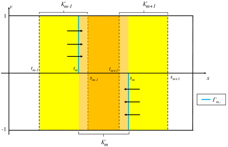
Figure 6: Domain decomposition for nonlinear RTE and the incoming boundary of the local patch.

In this particular setup, according to [72], if $\phi$ is in the space

$$\mathcal{X}=L^{2}(\Gamma_{-})\times\mathbb{R}_{+}^{2}=\left\{\left(g,\theta^{(1)},\theta^{(2)}\right)\mid g\in L^{2}(\Gamma_{-});\;\theta^{(1)},\theta^{(2)}\geq 0\right\}\,,$$

then there exists a unique positive solution in the space

$$\mathcal{Y}=H_{2}^{1}(\mathcal{K})\times H^{1}(\mathcal{D})=\left\{(I,T)\mid I\in H_{2}^{1}(\mathcal{K}),T\in H^{1}(\mathcal{D})\right\}\,,$$

where $H_{2}^{1}(\mathcal{K})$ is the space of functions for which the following norm is finite:

$$\|I\|_{H_{2}^{1}(\mathcal{K})}=\|I\|_{L^{2}(\mathcal{K})}+\|v\partial_{x}I\|_{L^{2}(\mathcal{K})}\,.$$

Note that the trace operators $T_{\pm}u=u|_{\Gamma_{\pm}}$ are well-defined maps from $H_{2}^{1}(\mathcal{K})$ to $L^{2}(\Gamma_{\pm})$ (see, for example [6]).

To proceed, we define several operators. We denote spaces associated with each patch $m$ as follows:

$$\mathcal{X}_{m} :=L^{2}(\Gamma_{m,-})\times\mathbb{R}_{+}^{2}=\left\{\left(g,\theta^{(1)},\theta^{(2)}\right)\mid g\in L^{2}(\Gamma_{m,-}),\;\theta^{(1)},\theta^{(2)}\geq 0\right\}\,,$$

$$\mathcal{Y}_{m} :=H_{2}^{1}(\mathcal{K}_{m})\times H^{1}(\mathcal{D}_{m})=\left\{(I,T)\mid I\in H_{2}^{1}(\mathcal{K}_{m}),\;T\in H^{1}(\mathcal{D}_{m})\right\}\,.$$

Then we have the following operator definitions for each patch $m$. (For simplicity of notation, we set $\sigma\equiv 1$ in the definition (33) of $B(T)$.)

• The solution operator $\mathcal{S}_{m}:\mathcal{X}_{m}\to\mathcal{Y}_{m}$ satisfies $\mathcal{S}_{m}\phi_{m}=u_{m}$, where $u_{m}=(I_{m}^{\epsilon},T_{m}^{\epsilon})$ solves the RTE on patch $\mathcal{K}_{m}$ with boundary condition
  $\phi_{m}=(g_{m},\theta_{m}^{(1)},\theta_{m}^{(1)})$:

  $$\begin{cases}\epsilon v\partial_{x}I_{m}^{\epsilon}&=(T_{m}^{\epsilon})^{4}-I_{m}^{\epsilon}\\ \epsilon^{2}\partial_{x}^{2}T_{m}^{\epsilon}&=(T_{m}^{\epsilon})^{4}-\langle I_{m}^{\epsilon}\rangle\end{cases}\,,\;(x,v)\in\mathcal{K}_{m}\,,$$

  with $T_{m}^{\epsilon}(t_{m})=\theta_{m}^{(1)}$, $T_{m}^{\epsilon}(s_{m})=\theta_{m}^{(2)}$, and

  $$I_{m}^{\epsilon}|_{\Gamma_{m,-}}=g_{m}(x,v)=(g_{m}^{(1)}(x,v),g_{m}^{(2)}(x,v))\,.$$

• The restriction operator $\mathcal{I}_{m\pm 1}^{m}$ from patch $\mathcal{K}_{m}$ to the boundaries of adjacent patches, namely, $\mathcal{K}_{m}\cap\Gamma_{m\pm 1,-}$ and $\mathcal{D}_{m}\cap\partial\mathcal{D}_{m\pm 1,-}$, is defined as follows:

  $$\mathcal{I}_{m+1}^{m}u_{m}=(I_{m}^{\epsilon}|_{\mathcal{K}_{m}\cap\Gamma_{m+1,-}},T_{m}^{\epsilon}|_{\mathcal{D}_{m}\cap\partial\mathcal{D}_{m+1,-}}),\quad m=1,\dotsc,M-1\,,$$

  $$\mathcal{I}_{m-1}^{m}u_{m}=(I_{m}^{\epsilon}|_{\mathcal{K}_{m}\cap\Gamma_{m-1,-}},T_{m}^{\epsilon}|_{\mathcal{D}_{m}\cap\partial\mathcal{D}_{m-1,-}}),\quad m=2,\dotsc,M\,.$$

• The boundary update operator $\mathcal{P}_{m}:\mathcal{X}_{m-1}\oplus\mathcal{X}_{m+1}\rightarrow\mathcal{X}_{m}$ is defined for $m\neq 1$ and $m\neq M$ by

  (45) $$\mathcal{P}_{m}(\phi_{m-1},\phi_{m+1})=(\mathcal{I}_{m}^{m-1}\mathcal{S}_{m-1}\phi_{m-1},\mathcal{I}_{m}^{m+1}\mathcal{S}_{m+1}\phi_{m+1}).$$

  For the two “end” patches $\mathcal{K}_{1}$ and $\mathcal{K}_{M}$ that intersect with physical boundary $\Gamma_{-}$, boundary conditions are updated only in the interior of the domain:

  $$\mathcal{P}_{1} :\mathcal{X}\times\mathcal{X}_{2}\rightarrow\mathcal{X}_{1},\quad \mathcal{P}_{1}(\phi,\phi_{2}) =(\phi|_{\Gamma_{-}\cap\Gamma_{1,-}},\mathcal{I}_{1}^{2}\mathcal{S}_{2}\phi_{2})\,,$$

  $$\mathcal{P}_{M} :\mathcal{X}_{M-1}\times\mathcal{X}\rightarrow\mathcal{X}_{M},\quad \mathcal{P}_{M}(\phi_{M-1},\phi) =(\mathcal{I}_{M}^{M-1}\mathcal{S}_{M-1}\phi_{M-1},\phi|_{\Gamma_{-}\cap\Gamma_{M,-}})\,.$$

As suggested by Algorithm 1, in the offline stage, we construct local dictionaries on interior patches from a few random samples, enlarging each interior patch slightly to eliminate the boundary layer effect. Define $\widetilde{\mathcal{K}}_{m}$ and $\widetilde{\mathcal{D}}_{m}$ such that

$$\mathcal{K}_{m}\subset\widetilde{\mathcal{K}}_{m}=\widetilde{\mathcal{D}}_{m}\times\mathcal{V}\,,$$

where $\mathcal{D}_{m}\subset\widetilde{\mathcal{D}}_{m}\subset\mathcal{D}$ expands the boundary of $\mathcal{D}_{m}$ to both sides by a margin of $\Delta x_{\text{b}}$. Denoting by $\widetilde{\Gamma}_{m,-}$ the boundary coordinates corresponding to $\widetilde{\mathcal{D}}_{m}$, we let $\widetilde{\mathcal{X}}_{m}=L^{2}(\widetilde{\Gamma}_{m,-})\times\mathbb{R}^{2}$ capture the boundary conditions on $\partial\widetilde{\mathcal{D}}_{m}$.

We draw $N$ samples $\widetilde{\phi}_{m,i}$, $i=1,2,\dotsc,N$, randomly from the set

$$B_{+}(R_{m};\widetilde{\mathcal{X}}_{m}):=\{\widetilde{\phi}=(\widetilde{I}_{B},\widetilde{T}_{B})\in\widetilde{\mathcal{X}}_{m}:\|\widetilde{\phi}\|_{\widetilde{\mathcal{X}}_{m}}\leq R_{m},\;\widetilde{I}_{B}\geq 0,\;\widetilde{T}_{B}\geq 0\}\,.$$

(The sampling procedure is discussed in in Appendix B.) The local solutions $\widetilde{u}_{m,i}=(\widetilde{I}_{m,i}^{\epsilon},\widetilde{T}_{m,i}^{\epsilon})$ solve

(46) $$\begin{cases}\epsilon v\partial_{x}\widetilde{I}_{m,i}^{\epsilon}=(\widetilde{T}_{m,i}^{\epsilon})^{4}-\widetilde{I}_{m,i}^{\epsilon}\\ \epsilon^{2}\partial_{x}^{2}\widetilde{T}_{m,i}^{\epsilon}=(\widetilde{T}_{m,i}^{\epsilon})^{4}-\langle\widetilde{I}_{m,i}^{\epsilon}\rangle\end{cases}\;\;(x,v)\in\widetilde{\mathcal{K}}_{m}\,,$$

$$\quad(\widetilde{I}_{m,i}^{\epsilon}|_{\widetilde{\Gamma}_{m,-}},\widetilde{T}_{m,i}^{\epsilon}|_{\partial\widetilde{\mathcal{D}}_{m}})=\widetilde{\phi}_{m,i}\,,\quad i=1,2,\dotsc,N.$$

The solutions to these equations, confined to the original patch $\mathcal{K}_{m}$ and its boundary $\Gamma_{m}$, are used to construct two dictionaries:

(47) $$\mathscr{I}_{m}=\{\psi_{m,i}\}_{i=1}^{N},\quad\mathscr{B}_{m}=\{\phi_{m,i}\}_{i=1}^{N}.$$

where

$$\psi_{m,i}=(\widetilde{I}_{m,i}^{\epsilon}|_{\mathcal{K}_{m}},\widetilde{T}_{m,i}^{\epsilon}|_{\mathcal{D}_{m}})\,,\quad\phi_{m,i}=(\widetilde{I}_{m,i}^{\epsilon}|_{\Gamma_{m,-}},\widetilde{T}_{m,i}^{\epsilon}|_{\partial\mathcal{D}_{m}})\,.$$

In the online stage, at each iteration, we seek neighbors to interpolate for local solutions. We use the $L^{2}$ norm to measure the distance between the newly generated solutions and the older solution set. Denote by $\phi_{m}^{(n)}$ the solution at the $n$-th iteration in patch $\mathcal{K}_{m}$, and define by

$$\{\phi_{m,i_{q}^{(n)}}\,,\quad q=1,2,\dotsc,k\}$$

its $k$ nearest neighbors in $\mathscr{B}_{m}$, for some chosen positive integer $k$, with the indices $i_{q}^{(n)}$ being ordered so that $\phi_{m,i_{1}^{(n)}}$ is the nearest neighbor. Then we define the local tangential approximation $\mathcal{S}_{m}\phi_{m}^{(n)}$ by:

(48) $$u_{m}^{(n)}=\mathcal{S}_{m}\phi_{m}^{(n)}=\psi_{m,i_{1}^{(n)}}+\Psi_{m}^{(n)}c_{m}^{(n)}\,,$$

where $\Psi_{m}^{(n)}$ and $c_{m}^{(n)}$ are defined as in Eq. 12 and Eq. 13. The local solution is then updated as follows:

(49) $$\phi_{m}^{(n+1)}=\mathcal{P}_{m}(\phi_{m-1}^{(n)},\phi_{m+1}^{(n)})=(\mathcal{I}_{m}^{m-1}\mathcal{S}_{m-1}\phi_{m-1}^{(n)},\mathcal{I}_{m}^{m+1}\mathcal{S}_{m+1}\phi_{m+1}^{(n)})\,.$$

For $m=1$ and $m=M$, to avoid updating the physical boundary, we set

$$\mathcal{P}_{1}(\phi,\phi_{2}^{(n)}) =(\phi|_{\Gamma_{-}\cap\Gamma_{1,-}},\mathcal{I}_{1}^{2}\mathcal{S}_{2}\phi_{2}^{(n)})\,,$$

$$\mathcal{P}_{M}(\phi_{M-1}^{(n)},\phi) =(\mathcal{I}_{M}^{M-1}\mathcal{S}_{M-1}\phi_{M-1}^{(n)},\phi|_{\Gamma_{-}\cap\Gamma_{M,-}})\,.$$

Once the convergence is achieved (at iteration $n$, say), we assemble the final solution as

(50) $$u_{\text{final}}=u^{(n)}=\sum_{m=1}^{M}\chi_{m}u_{m}^{(n)}\,,$$

with $\chi_{m}:\Omega\rightarrow\mathbb{R}$ being the smooth partition of unity associated with the partition of $\mathcal{K}$.

4.4 Numerical Tests

In the numerical tests, we take the domain to be

$$\mathcal{K}=\mathcal{D}\times\mathcal{V}=[0,L]\times[-1,1]=[0,3]\times[-1,1].$$

To form the patch $\mathcal{K}_{m}=\mathcal{D}_{m}\times\mathcal{V}$, the domain $\mathcal{D}$ is divided into $M=7$ non-overlapping patches whose widths are $d_{1}=d_{7}=\tfrac{L}{2(M-1)}=0.25$ and $d_{i}=\tfrac{L}{M-1}=0.5$, $i=2,\cdots,M-1$. Each patch is then enlarged by $\Delta x_{\text{o}}=.125$ to both sides (except the ones adjacent to the physical boundary, which are enlarged only on the “internal” sides), so we have

$$\mathcal{D}_{m}=\left(\tfrac{L(2m-1)}{2(M-1)}-\Delta x_{\text{o}},\tfrac{L(2m-1)}{M}+\Delta x_{\text{o}}\right)\,,\;\;m=2,\dots,M-1\,,$$

$$\mathcal{D}_{1}=\left(0,\tfrac{L}{2(M-1)}+\Delta x_{\text{o}}\right)\,,\quad\mathcal{D}_{M}=\left(L-\tfrac{3}{2(M-1)}-\Delta x_{\text{o}},3\right)\,.$$

The region of overlap between adjacent patches $\mathcal{K}_{m}$ has size $2\Delta x_{\text{o}}\times[-1,1]$. The partition of unity functions over each patch $\mathcal{K}_{m}$ are obtained using the method of Section 3.4

Denote the spatial grid points by $0=x_{0}<x_{1}<\cdots<x_{N_{x}-1}<x_{N_{x}}=L$, which is a uniform grid with step size $\Delta x=\tfrac{L}{N_{x}}$. The velocity grid points are denoted by $-1<v_{1}<v_{2}<\cdots<v_{N_{v}-1}<v_{N_{v}}<1$ for some even value of $N_{v}$. We use the Gauss-Legendre quadrature points for the $v_{i}$. The numerical solutions are denoted by $I^{ij}\approx I(x_{i},v_{j})$ and $T^{i}\approx T(x_{i})$. To quantify the numerical error, we denote the discrete $L^{2}$ norm of $u=([I^{ij}],[T^{i}])$ by

$$\|u\|^{2}_{2} =\sum_{j=1}^{N_{v}}w_{j}\frac{\Delta x}{2}|I^{0j}|^{2}+\sum_{j=1}^{N_{v}}w_{j}\frac{\Delta x}{2}|I^{iN_{x}}|^{2}+\sum_{i=1}^{N_{x}-1}\sum_{j=1}^{N_{v}}w_{j}\Delta x|I^{ij}|^{2}$$

$$\quad+\frac{\Delta x}{2}|T^{0}|^{2}+\frac{\Delta x}{2}|T^{N_{x}}|^{2}+\sum_{i=1}^{N_{x}-1}\Delta x|T^{i}|^{2}\,,$$

where $w_{j}$ is the Gauss-Legendre weight, and the relative error $u_{\text{ref}}$ between a reference solution and an approximate solution $u_{\text{approx}}$ is defined by

$$\text{relative }L^{2}\text{ error}=\frac{\|u_{\text{ref}}-u_{\text{approx}}\|_{2}}{\|u_{\text{ref}}\|_{2}}\,.$$

We solve the PDE using finite differences. The intensity equation is discretized in space by a classical second-order exponential finite difference scheme [61, 81], and the temperature equation is approximated by the standard three-point scheme. The resulting nonlinear system is then solved by fixed point iteration [69, 72], where in each evaluation of the fixed point map, the monotone iterative method is exploited to solve the semilinear elliptic equation. For computations with $\epsilon=2^{-4}$ and $\epsilon=2^{-6}$, we further use Anderson acceleration to boost the convergence of fixed point iteration [10, 45, 87].

We use extremely fine discretization with $\Delta x=2^{-14}=\tfrac{1}{16384}$ and $N_{v}=2^{10}=1024$. The discretization is fine enough for us to view it as the reference solution. All the other computations are done with coarser mesh $\Delta x=2^{-11}=\tfrac{1}{2048}$ and $N_{v}=2^{7}=128$.

The boundary condition $\phi=(g^{(1)},g^{(2)},\theta^{(1)},\theta^{(2)})$ is defined as follows:

$$g^{(1)}(0,v>0)=3+\sin(2\pi v)\,, \quad g^{(2)}(L=3,v<0)=2+\sin(2\pi v)\,,$$

$$\theta(0)=\theta^{(1)}=2\,, \quad\theta(L)=\theta^{(2)}=3\,.$$

The enlarged patches needed in the offline stage, denoted by $\widetilde{\mathcal{K}}_{m}$, are obtained by enlarging each respective $\mathcal{K}_{m}$ by the quantity $\Delta x_{\text{b}}$. The configuration of the domain and the partition are seen in Figure 7, where $\Delta x_{\text{b}}=.125$.

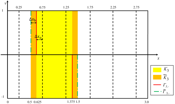
Figure 7: Configuration of patches (including enlarged patches) in the decomposed domain

On the buffered interior patch $\widetilde{\mathcal{K}}_{m}$, we sample $N=64$ configuration of boundary conditions in $B_{+}(R_{m};\widetilde{\mathcal{X}}_{m})$. On the discrete level, this process finds $64$ boundary conditions $\widetilde{\phi}$ so that

$$\|\widetilde{\phi}\|^{2}=\sum_{j=1}^{\frac{N_{v}}{2}}w_{j}|\widetilde{g}^{(2)}(s,v_{j})|^{2}+\sum_{j=\frac{N_{v}}{2}+1}^{N_{v}}w_{j}|\widetilde{g}^{(1)}(t,v_{j})|^{2}+|\widetilde{\theta}^{(1)}|^{2}+|\widetilde{\theta}^{(2)}|^{2}<R_{m}\,.$$

We set $R_{m}=25$ in our experiments.

To demonstrate the linearity of the updating map $\mathcal{P}_{m}$, we choose the patch $\mathcal{K}_{3}=[0.625,1.375]\times[-1,1]$, which overlaps $\mathcal{K}_{2}$ at $[0.625,0.875]\times[-1,1]$. For $\Delta x_{\text{b}}=2^{-3}$ and $\epsilon=2^{-6}$, we compute local solutions on the buffered domain $\widetilde{\mathcal{K}}_{3}$ with $64$ different configurations, and evaluate $T$ at $0.625$ and $1.375$ (the two ending points of $\mathcal{K}_{3}$) and at $0.875$ (the point that intersects with $\partial\mathcal{K}_{2}$). In Figure 8, we plot $T(0.875)$ as a function of $T(0.625)$ and $T(1.375)$. We observe that it is a slowly varying two-dimensional manifold and is locally almost linear. Thus, $T(0.875)$ can be determined uniquely by the pair of values $(T(0.625),T(1.375))$. Further, we plot $\tfrac{\langle|I(x,\cdot)-\langle I\rangle(x)|^{2}\rangle}{\langle I\rangle(x)^{2}}$ and $\tfrac{\langle I\rangle(x)-T^{4}(x)}{T^{4}(x)}$ at $x=0.875$, showing that the relative variation is nearly zero. This means that $I$ is essentially constant at $x=0.875$, with $I=T^{4}$. These calculations suggest that the entire solution on this patch is uniquely determined by $T(0.625)$ and $T(1.375)$, implying that the local degrees of freedom for the solution in the entire patch is only two, so that the local solution manifold is approximately two-dimensional.

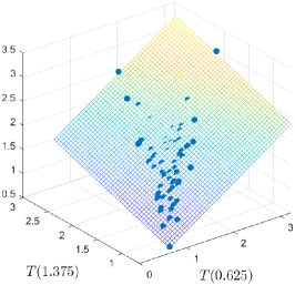
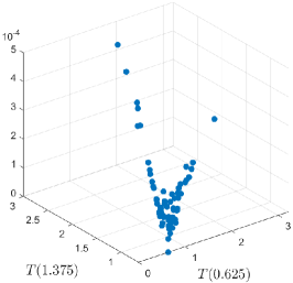
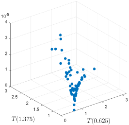
Figure 8: The plot on the left shows the point cloud $(T(0.625),T(1.375),T(0.875))$ and its fitting plane. We observe that the manifold is approximately two-dimensional, so that $T(0.875)$ can be uniquely determined by $(T(0.625),T(1.375))$. The middle and right panels show the quantities $\tfrac{\langle|I(x,\cdot)-\langle I\rangle(x)|^{2}\rangle}{\langle I\rangle(x)^{2}}$ and $\tfrac{\langle I\rangle(x)-T(x)^{4}}{T(x)^{4}}$ at $x=0.875$, respectively, showing that the solution is nearly constant, with $I=T^{4}$.

To verify that the local dictionary represents the solution manifold adequately, we confine the reference solution in patch $\mathcal{K}_{2}$ and project it onto the space spanned by its nearest $k$ modes in the local dictionary. We evaluate the resulting relative error as a function of $k$, plotting the result in Figure 9. For $\epsilon=2^{-6}$ and $\Delta x_{\text{b}}=.125$, we observe a sharp decay of error when $k\geq 3$, meaning that the local reference solution can be represented to acceptable accuracy by two local dictionary modes, and suggesting once again that the local solution manifold is two-dimensional.

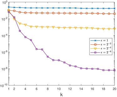
(a) $\Delta x_{\text{b}}=2^{-2}$

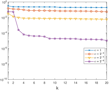
(b) $\Delta x_{\text{b}}=2^{-3}$

Figure 9: The relative error of the $L^{2}$ projection of the reference solution onto the space spanned by the nearest $k$ modes on the patch $\mathcal{K}_{2}$.

The sample number $N$ and the radius $R_{m}$ are two crucial parameters that affect the effectiveness of the method. We check how the approximation capability of the local dictionary depends on the two parameters over the local patch $\mathcal{K}_{2}$. In Figure 10a, we show the projection error as $N$ increases for different $R_{m}$. The error of the dictionary saturates as $N$ increases, and it can be used as a criterion to decide the size of the local dictionary. In Figure 10b, we show the relative projection error of the reference solution onto the local tangent space using dictionaries with different $R_{m}$. It can be seen that the radius $R_{m}$ must be large enough to obtain a good local basis.

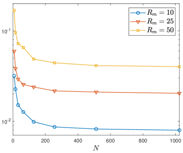
(a)

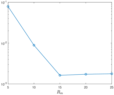
(b)

Figure 10: The plot on the left shows the average error of the $L^{2}$ projection of 100 test samples onto the space spanned by the nearest 5 modes. The test samples are generated from the same distribution as the dictionary. The plot on the right shows the relative error of the $L^{2}$ projection of the reference solution onto the space spanned by the nearest 5 modes on patch $\mathcal{K}_{2}$. The number of samples is $N=64$ for all $R_{m}$.

In the online computation, we set the stopping criterion to be

$$\sum_{m}\|\phi_{m}^{(n)}-\phi_{m}^{(n-1)}\|<10^{-3}\,,$$

where $\phi_{m}^{(n)}$ is the boundary condition on the patch $\mathcal{K}_{m}$ at the $n$-th iteration. We take the initial boundary condition on each patch to be trivial, setting $\phi_{m}^{(0)}|_{\Gamma_{m,-}\backslash\Gamma_{-}}=0$, except on the real physical boundary condition, where it is set to the prescribed Dirichlet conditions.

In Figure 11, we compare the reference solution with our numerical solution computed using $k=5$ and buffer zone $\Delta x_{\text{b}}=2^{-3}$. When $\epsilon=1$, the equation is far away from its homogenization limit, and the numerical solution is far from the reference, but for $\epsilon=2^{-6}$ the numerical solution is captured rather well using just $k=5$ neighbors.

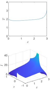
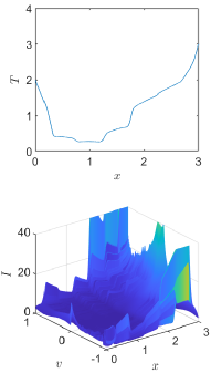
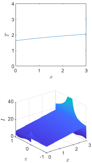
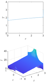
Figure 11: The first two columns of plots show the reference solution and numerical solution for $\epsilon=1$, and the last two columns compare the solutions for $\epsilon=2^{-6}$.

In Figure 12 we document the relative error for various values of $k$ and $\Delta x_{\text{b}}$. When $\epsilon$ is small, and for buffer width $\Delta x_{\text{b}}$ sufficiently large, we need only $k=2$ neighbors to produce a solution of acceptable accuracy. Without the buffer zone to damp the boundary layer effect, however, the low dimensionality of the solution manifold cannot be captured, even for small $\epsilon$.

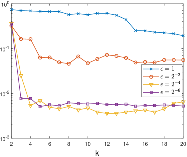
(a) $\Delta x_{\text{b}}=2^{-2}$

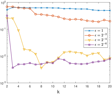
(b) $\Delta x_{\text{b}}=2^{-3}$

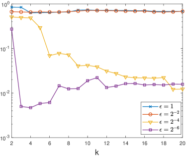
(c) $\Delta x_{\text{b}}=2^{-4}$

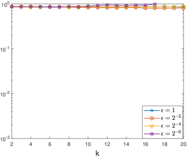
(d) $\Delta x_{\text{b}}=0$

Figure 12: The relative $L^{2}$ error in one trial as a function of $k$, for various values of $\Delta x_{\text{b}}$ and $\epsilon$.

We also compare the cost of our reduced method with the classical Schwarz iteration. CPU times for both methods are summarized in Table 2 for $\epsilon=2^{-4}$ and $\epsilon=2^{-6}$, with buffer size $\Delta x_{\text{b}}=.125$. The online cost of the reduced method is about $1000$ times cheaper than the classical Schwarz iteration when $\epsilon=2^{-4}$ and $4000$ times cheaper when $\epsilon=2^{-6}$. Even considering the large overhead cost in the offline stage, the reduced order method is still cheaper than Schwarz iteration.

	CPU Time (s)
	$\epsilon=2^{-4}$		$\epsilon=2^{-6}$
	offline	online	offline	online
Reduced model $k=3$	394.3911	0.181324	904.7498	0.215390
Reduced model $k=5$		0.301761		0.222538
Reduced model $k=10$		0.379348		0.282070
Reduced model $k=15$		0.548689		0.346633
Reduced model $k=20$		0.586276		0.532603
Classical Schwarz	—	458.0987	—	2183.7079

Table 2: CPU time comparison between reduced model method with $k=3,5,10,15,20$ (size of each local dictionary $N=64$).

Finally, we reiterate that due to the nonlinear nature of the equations, the concept of “basis function” is not well defined. The reduced model method for linear equations was proposed in [26, 28], where random sampling is used to construct the boundary-to-boundary map $\mathcal{P}$, by following the idea of randomized SVD [54]. If we translate this approach to nonlinear homogenization, using Green’s functions in a brute-force manner, the numerical results are poor. By the “Green’s functions,” we mean the solution to the equation with delta boundary conditions (counterparts of Green’s functions in the linear setting). The numerical results are presented in Figure 13, that compares the ground-truth solution with the Green’s function interpolation.

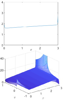
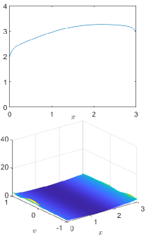
Figure 13: The left column of plots is the solution with $\epsilon=2^{-4}$, and the right column is the solution from a linear combination of the full set of “Green’s functions”.

5 Conclusion

Multiscale physical phenomena are often described by PDEs that contain small parameters. it is generally expensive to capture small-scale effects using numerical solvers. There is a vast literature on improving numerical performance of PDE solvers in this context, but most algorithms are equation-specific, requiring analytical understanding to be built into algorithm design.

We have described numerical methods that can capture the homogenization limit of nonlinear PDEs with small scales automatically, without analytical prior knowledge. This work can be seen as a nonlinear extension of our earlier work [27] for linear PDEs. Elements of our algorithm include domain decomposition framework and Schwarz iteration. The method is decomposed into offline and online stages, where in the offline stage, random sampling is employed to learn the low-rank structure of the solution manifold, while in the online stage, the reduced manifolds serve as surrogates of local solvers in the Schwarz iteration. Since the manifolds are prepared offline and are of low dimension, the method exhibits significant speedup over naive approaches, as we demonstrate using computational results on two examples.

Appendix A Sampling method for the semilinear elliptic equation

We explain here the sampling method for the semilinear elliptic equation in Section 3.4. To enforce the boundary condition on the physical boundary, patches that intersect this boundary should be treated differently from patches inside the domain. (We call the patch $\widetilde{\Omega}_{m}$ an “interior patch” if it satisfies $\partial\widetilde{\Omega}_{m}\cap\partial\Omega=\varnothing$, and a “boundary patch” otherwise.)

A.1 Sampling for interior patches

For the interior patch $\partial\widetilde{\Omega}_{m}$, each sample in $B(R_{m};\,\widetilde{\mathcal{X}}_{m})$ is decomposed into radial and angular parts $\widetilde{\phi}=rX$, with the two parts $r$ and $X$ sampled independently. The radial part $r$ is generated so that $(\frac{r}{R_{m}})^{D}$ is uniformly distributed in the unit interval $[0,1]$, where $D$ is a preset integer. (We choose $D=5$ and $R_{m}=R=20$ in our tests.) The angular part $X$ is a $N_{m}$-dimensional vector uniformly distributed in the set $\{X\in\mathbb{R}^{N_{m}}:\|X\|_{1/2}=1\}$, where $N_{m}$ is the number of grid points on $\partial\widetilde{\Omega}_{m}$, and the norm $\|\cdot\|_{1/2}$ is defined by

$$\|\widetilde{\phi}\|_{1/2}=\sqrt{h\sum_{i=1}^{N_{m}}|\widetilde{\phi}_{i}|^{2}+h^{2}\sum_{\begin{subarray}{c}i,j=1\\ i\neq j\end{subarray}}^{N_{m}}\frac{|\widetilde{\phi}_{i}-\widetilde{\phi}_{j}|^{2}}{|z_{i}-z_{j}|^{2}}}\,.$$

Here $\widetilde{\phi}=(\widetilde{\phi}_{i})_{i=1}^{N_{m}}$ is any discrete boundary condition, and $z_{i}$ denotes the grid point on $\partial\widetilde{\Omega}_{m}$.

In order to generate $X$, let $Y_{1},\dotsc,Y_{N_{m}}\sim\mathcal{N}(0,1)$ be i.i.d. standard Gaussian random variables. Define the weight matrix $W=(W_{ij})_{N_{m}\times N_{m}}$ by

$$W_{ii}=h+\sum_{\begin{subarray}{c}j=1\\ j\neq i\end{subarray}}^{N_{m}}\tfrac{2h^{2}}{|z_{i}-z_{j}|^{2}}\,,\quad W_{ij}=-\tfrac{2h^{2}}{|z_{i}-z_{j}|^{2}}\,,$$

and suppose that its Cholesky decomposition is $W=C^{\top}C$. Then the vector $Z=C^{-1}(Y_{1},\cdots,Y_{N_{m}})^{\top}$ has uniform angular distribution with respect to the norm $\|\cdot\|_{1/2}$, so its normalization $X=\tfrac{Z}{\|Z\|_{1/2}}$ is uniformly distributed on the unit sphere $\{X\in\mathbb{R}^{N_{m}}:\|X\|_{1/2}=1\}$.

A.2 Sampling for boundary patches

Let

$$\widetilde{\phi}_{m}=\begin{bmatrix}\widetilde{\phi}_{m,d}\\ \widetilde{\phi}_{m,r}\end{bmatrix}\in\mathbb{R}^{N_{m}}$$

be a random sample, with $\widetilde{\phi}_{m,d}$ representing the physical boundary part and $\widetilde{\phi}_{m,r}$ representing the random part. When we rearrange the weight matrix $W$ as

$$W=\begin{bmatrix}W_{dd}&W_{dr}\\ W_{rd}&W_{rr}\end{bmatrix}\,,$$

so that $\|\widetilde{\phi}_{m}\|^{2}_{1/2}=\widetilde{\phi}_{m}^{\top}W\widetilde{\phi}_{m}$, then it yields

$$\widetilde{\phi}_{m,r}^{\top}W_{rr}\widetilde{\phi}_{m,r}=R_{m}^{2}-\widetilde{\phi}_{m,d}^{\top}(W_{dd}-W_{dr}W_{rr}^{-1}W_{rd})\widetilde{\phi}_{m,d}\,,$$

indicating that the random part lies in a ellipsoid.

Hence, the random part $\widetilde{\phi}_{m,r}$ can be sampled as follows. We decompose it into independently sampled radial and angular part $\widetilde{\phi}_{r}=r_{m}X_{m}$, so that $r_{m}^{D}$ is uniformly distributed in the interval $\left[0,(R_{m}^{2}-\widetilde{\phi}_{m,d}^{\top}(W_{dd}-W_{dr}W_{rr}^{-1}W_{rd})\widetilde{\phi}_{m,d})^{D/2}\right]$, and $X_{m}$ is uniformly distributed on the set $\{X_{m}:X_{m}^{\top}W_{rr}X_{m}=1\}$.

Appendix B Sampling method for the nonlinear radiative transfer equations

Here we describe the sampling method for the nonlinear radiative transfer equations discussed in Section 4.4.

To generate samples for the interior patches $\widetilde{\mathcal{K}}_{m}$, $m=2,\cdots,M-1$, each sample is decomposed into radial and angular parts $\widetilde{\phi}=rX$, which are sampled independently. We take $(\frac{r}{R_{m}})^{2}$ to be uniformly distributed in $[0,1]$, while $X$ is a $(N_{v}+2)$-dimensional vector uniformly distributed in the set $\{X\in\mathbb{R}^{N_{v}+2}:\|X\|=1,X\geq 0\}$, where the norm $\|\cdot\|$ is defined by

$$\|\widetilde{\phi}\|^{2}=\sum_{j=1}^{\frac{N_{v}}{2}}w_{j}|\widetilde{g}^{(2)}(s,v_{j})|^{2}+\sum_{j=\frac{N_{v}}{2}+1}^{N_{v}}w_{j}|\widetilde{g}^{(1)}(t,v_{j})|^{2}+|\widetilde{\theta}^{(1)}|^{2}+|\widetilde{\theta}^{(2)}|^{2}\,,$$

given any discrete boundary condition

$$\widetilde{\phi}=\left(\{\widetilde{g}^{(2)}(s,v_{j})\}_{j=1}^{\frac{N_{v}}{2}},\{\widetilde{g}^{(1)}(t,v_{j})\}_{j=\frac{N_{v}}{2}+1}^{N_{v}},\widetilde{\theta}^{(1)},\widetilde{\theta}^{(2)}\right).$$

Here $N_{v}$ is the number of grid points in the velocity direction and the $w_{j}$ are the Gaussian-Legendre weights. (We choose $R_{m}=R=25$ in our tests.)

To generate $X$, let $Y_{1},\dotsc,Y_{N_{v}+2}\sim\mathcal{N}(0,1)$ be i.i.d. standard Gaussian random variables. Denote the vector

$$Z=\left(\frac{Y_{1}}{\sqrt{w_{1}}},\cdots,\frac{Y_{N_{v}}}{\sqrt{w_{N_{v}}}},Y_{N_{v}+1},Y_{N_{v}+2}\right)\,.$$

Then the normalized vector $X=\frac{Z}{\|Z\|}$ is uniformly distributed on the unit sphere $\{X\in\mathbb{R}^{N_{v}+2}:\|X\|=1\}$. Note that (46) is invariant under $x$-translation, so we need only learn one interior dictionary on one interior patch, then re-use in for the other interior patches.

Sampling the boundary conditions on the boundary patches can be done in the same way. However, we do adjust the radius $r$. In particular, $(\frac{r}{R_{1/M}})^{2}$ is chosen uniformly in $[0,1]$, where $R_{1/M}$ has the fixed boundary condition deducted from $R$.

References

- [1] N. Abdallah, M. Puel, and M. Vogelius, Diffusion and homogenization limits with separate scales, Multiscale Model. Simul., 10 (2012), pp. 1148–1179.
- [2] A. Abdulle and Y. Bai, Reduced basis finite element heterogeneous multiscale method for high-order discretizations of elliptic homogenization problems, J. Comput. Phys., 231 (2012), pp. 7014 – 7036.
- [3] A. Abdulle, Y. Bai, and G. Vilmart, Reduced basis finite element heterogeneous multiscale method for quasilinear elliptic homogenization problems, Discrete Contin. Dyn. Syst. Ser. S, 8 (2015), pp. 91–118.
- [4] A. Abdulle and C. Schwab, Heterogeneous multiscale FEM for diffusion problems on rough surfaces, Multiscale Model. Simul., 3 (2005), pp. 195–220.
- [5] A. Abdulle and G. Vilmart, Analysis of the finite element heterogeneous multiscale method for quasilinear elliptic homogenization problems, Math. Comp., 83 (2014), pp. 513–536.
- [6] V. Agoshkov, Boundary Value Problems for Transport Equations, Springer Science & Business Media, 2012.
- [7] G. Allaire, Homogenization and two-scale convergence, SIAM J. Math. Anal., 23 (1992), pp. 1482–1518.
- [8] W. K. Allard, G. Chen, and M. Maggioni, Multi-scale geometric methods for data sets II: Geometric multi-resolution analysis, Appl. Comput. Harmon. Anal., 32 (2012), pp. 435–462.
- [9] H. Amann and J. Moser, On the existence of positive solutions of nonlinear elliptic boundary value problems, Indiana Univ. Math. J., 21 (1971), pp. 125–146.
- [10] D. G. Anderson, Iterative procedures for nonlinear integral equations, J.ACM, 12 (1965), pp. 547–560.
- [11] A. Andoni, P. Indyk, and I. Razenshteyn, Approximate nearest neighbor search in high dimensions, arXiv preprint arXiv:1806.09823, 7 (2018).
- [12] I. Babuška and R. Lipton, Optimal local approximation spaces for generalized finite element methods with application to multiscale problems, Multiscale Model. Simul., 9 (2011), pp. 373–406.
- [13] I. Babuška and J. M. Melenk, The partition of unity method, Internat. J. Numer. Methods Engrg., 40 (1997), pp. 727–758.
- [14] C. Bardos, F. Golse, and D. Levermore, Fluid dynamic limits of kinetic equations. I. Formal derivations, J. Stat. Phys., 63 (1991), pp. 323–344.
- [15] C. Bardos, F. Golse, and B. Perthame, The Rosseland approximation for the radiative transfer equations, Comm. Pure Appl. Math., 40 (1987), pp. 691–721.
- [16] C. Bardos, F. Golse, B. Perthame, and R. Sentis, The nonaccretive radiative transfer equations: existence of solutions and Rosseland approximation, J. Funct. Anal., 77 (1988), pp. 434–460.
- [17] C. Bardos, R. Santos, and R. Sentis, Diffusion approximation and computation of the critical size, Trans. Amer. Math. Soc., 284 (1984), pp. 617–649.
- [18] M. Bebendorf, Why finite element discretizations can be factored by triangular hierarchical matrices, SIAM J. Numer. Anal., 45 (2007), pp. 1472–1494.
- [19] M. Belkin and P. Niyogi, Laplacian eigenmaps and spectral techniques for embedding and clustering, in Adv. in Neural Inform. Process. Systems, 2002, pp. 585–591.
- [20] A. Bensoussan, L. Boccardo, and F. Murat, H convergence for quasi-linear elliptic equations with quadratic growth, Appl. Math. Optim., 26 (1992), pp. 253–272.
- [21] A. Bensoussan, J.-L. Lions, and G. Papanicolaou, Boundary layers and homogenization of transport processes, Publ. Res. Inst. Math. Sci., 15 (1979), pp. 53–157.
- [22] A. Bensoussan, J.-L. Lions, and G. Papanicolaou, Asymptotic Analysis for Periodic Structures, vol. 374, American Mathematical Soc., 2011.
- [23] A. Buhr and K. Smetana, Randomized local model order reduction, SIAM Journal on Scientific Computing, 40 (2018), pp. A2120–A2151.
- [24] S. Chandrasekhar, An introduction to the study of stellar structure, vol. 2, Courier Corporation, 1957.
- [25] K. Chen, Q. Li, and J. G. Liu, Online learning in optical tomography: a stochastic approach, Inverse Problems., 34 (2018), p. 075010.
- [26] K. Chen, Q. Li, J. Lu, and S. J. Wright, Random sampling and efficient algorithms for multiscale PDEs, arXiv preprint arXiv:1807.08848, (2018).
- [27] K. Chen, Q. Li, J. Lu, and S. J. Wright, Randomized sampling for basis functions construction in generalized finite element methods, arXiv preprint arXiv:1801.06938, (2018).
- [28] K. Chen, Q. Li, J. Lu, and S. J. Wright, A low-rank Schwarz method for radiative transport equation with heterogeneous scattering coefficient, arXiv preprint arXiv:1906.02176, (2019).
- [29] Z. Chen and T. Y. Savchuk, Analysis of the multiscale finite element method for nonlinear and random homogenization problems, SIAM J. Numer. Anal., 46 (2008), pp. 260–279.
- [30] M. Chipot, Elliptic Qquations: An Introductory Course, Springer, 2009.
- [31] E. T. Chung, Y. Efendiev, W. T. Leung, and M. Wheeler, Nonlinear nonlocal multicontinua upscaling framework and its applications, International Journal for Multiscale Computational Engineering, 16 (2018).
- [32] E. T. Chung, Y. Efendiev, W. T. Leung, and Z. Zhang, Cluster-based generalized multiscale finite element method for elliptic PDEs with random coefficients, J. Comput. Phys., 371 (2018), pp. 606–617.
- [33] R. R. Coifman, S. Lafon, A. B. Lee, M. Maggioni, B. Nadler, F. Warner, and S. W. Zucker, Geometric diffusions as a tool for harmonic analysis and structure definition of data: Diffusion maps, Proc. Natl. Acad. Sci. USA, 102 (2005), pp. 7426–7431.
- [34] P. Degond, Asymptotic-preserving schemes for fluid models of plasmas, CEMRACS 2010: Numerical methods for fusion, arXiv preprint arXiv:1104.1869, (2011).
- [35] E. Di Nezza, G. Palatucci, and E. Valdinoci, Hitchhiker’s guide to the fractional Sobolev spaces, Bull. Sci. Math., 136 (2012), pp. 521–573.
- [36] G. Dimarco and L. Pareschi, High order asymptotic-preserving schemes for the Boltzmann equation, C. R. Math. Acad. Sci. Paris, 350 (2012), pp. 481–486.
- [37] G. Dimarco and L. Pareschi, Numerical methods for kinetic equations, Acta Numer., 23 (2014), pp. 369–520.
- [38] L. Dumas and F. Golse, Homogenization of transport equations, SIAM J. Appl. Math., 60 (2000), pp. 1447–1470.
- [39] W. E and B. Engquist, The heterogeneous multiscale methods, Commun. Math. Sci., 1 (2003), pp. 87–132.
- [40] W. E, P. Ming, and P. Zhang, Analysis of the heterogeneous multiscale method for elliptic homogenization problems, J. Amer. Math. Soc., 18 (2005), pp. 121–156.
- [41] Y. Efendiev, J. Galvis, G. Li, and M. Presho, Generalized multiscale finite element methods. Nonlinear elliptic equations, Commun. Comput. Phys., 15 (2014), pp. 733–755.
- [42] Y. Efendiev and T. Y. Hou, Multiscale finite element methods: theory and applications, vol. 4, Springer Science & Business Media, 2009.
- [43] Y. Efendiev, T. Y. Hou, and V. Ginting, Multiscale finite element methods for nonlinear problems and their applications, Commun. Math. Sci., 2 (2004), pp. 553–589.
- [44] Y. R. Efendiev, T. Y. Hou, and X.-H. Wu, Convergence of a nonconforming multiscale finite element method, SIAM J. Numer. Anal., 37 (2000), pp. 888–910.
- [45] H.-R. Fang and Y. Saad, Two classes of multisecant methods for nonlinear acceleration, Numer. Linear Algebra Appl., 16 (2009), pp. 197–221.
- [46] F. Filbet and S. Jin, A class of asymptotic-preserving schemes for kinetic equations and related problems with stiff sources, J. Comput. Phys., 229 (2010), pp. 7625–7648.
- [47] F. Filbet and S. Jin, An asymptotic preserving scheme for the ES-BGK model of the Boltzmann equation, J. Comput. Phys., 46 (2011), pp. 204–224.
- [48] P. Gérard, P. Markowich, N. Mauser, and F. Poupaud, Homogenization limits and Wigner transforms, Comm. Pure Appl. Math., 50 (1997), pp. 323–379.
- [49] D. Gilbarg and N. Trudinger, Elliptic Partial Differential Equations of Second Order, Springer, 2015.
- [50] T. Goudon and A. Mellet, Diffusion approximation in heterogeneous media, Asymptot. Anal., 28 (2001), pp. 331–358.
- [51] T. Goudon and A. Mellet, Homogenization and diffusion asymptotics of the linear Boltzmann equation, ESAIM Control Optim. Calc. Var., 9 (2003), pp. 371–398.
- [52] Y. Guo and L. Wu, Geometric correction in diffusive limit of neutron transport equation in 2D convex domains, Arch. Ration. Mech. Anal., 226 (2017), pp. 321–403.
- [53] W. Hackbusch, Hierarchical matrices: algorithms and analysis, vol. 49, Springer, Heidelberg, 2015.
- [54] N. Halko, P.-G. Martinsson, and J. A. Tropp, Finding structure with randomness: Probabilistic algorithms for constructing approximate matrix decompositions, SIAM Rev., 53 (2011), pp. 217–288.
- [55] P. Henning, A. Målqvist, and D. Peterseim, A localized orthogonal decomposition method for semi-linear elliptic problems, ESAIM Math. Model. Numer. Anal., 48 (2014), pp. 1331–1349.
- [56] T. Y. Hou, F.-N. Hwang, P. Liu, and C.-C. Yao, An iteratively adaptive multi-scale finite element method for elliptic pdes with rough coefficients, Journal of Computational Physics, 336 (2017), pp. 375 – 400, https://doi.org/https://doi.org/10.1016/j.jcp.2017.02.002, http://www.sciencedirect.com/science/article/pii/S0021999117300955.
- [57] T. Y. Hou, Q. Li, and P. Zhang, Exploring the locally low dimensional structure in solving random elliptic pdes, Multiscale Modeling & Simulation, 15 (2017), pp. 661–695.
- [58] T. Y. Hou and X.-H. Wu, A multiscale finite element method for elliptic problems in composite materials and porous media, J. Comput. Phys., 134 (1997), pp. 169 – 189.
- [59] T. Y. Hou, X.-H. Wu, and Z. Cai, Convergence of a multiscale finite element method for elliptic problems with rapidly oscillating coefficients, Math. Comp., 68 (1999), pp. 913–943.
- [60] J. Hu, S. Jin, and Q. Li, Asymptotic-preserving schemes for multiscale hyperbolic and kinetic equations, in Handbook of Numerical Analysis, vol. 18, Elsevier, 2017, pp. 103–129.
- [61] A. M. Il’in, Differencing scheme for a differential equation with a small parameter affecting the highest derivative, Mathematical Notes of the Academy of Sciences of the USSR, 6 (1969), pp. 596–602.
- [62] P. Indyk and R. Motwani, Approximate nearest neighbors: towards removing the curse of dimensionality, in Proceedings of the thirtieth annual ACM symposium on Theory of computing, 1998, pp. 604–613.
- [63] S. Jin, Efficient asymptotic-preserving (AP) schemes for some multiscale kinetic equations, SIAM J. Sci. Comput., 21 (1999), pp. 441–454.
- [64] S. Jin and Q. Li, A BGK-penalization-based asymptotic-preserving scheme for the multispecies Boltzmann equation, Numer. Methods Partial Differential Equations, 29 (2013), pp. 1056–1080.
- [65] W. B. Johnson and J. Lindenstrauss, Extensions of Lipschitz mappings into a Hilbert space, Contemporary mathematics, 26 (1984), p. 1.
- [66] D. D. Joseph and T. S. Lundgren, Quasilinear Dirichlet problems driven by positive sources, Arch. Ration. Mech. Anal., 49 (1973), pp. 241–269.
- [67] S. Klainerman and A. Majda, Singular limits of quasilinear hyperbolic systems with large parameters and the incompressible limit of compressible fluids, Comm. Pure Appl. Math., 34 (1981), pp. 481–524.
- [68] S. Klainerman and A. Majda, Compressible and incompressible fluids, Comm. Pure Appl. Math., 35 (1982), pp. 629–651.
- [69] A. Klar and C. Schmeiser, Numerical passage from radiative heat transfer to nonlinear diffusion models, Math. Models Methods Appl. Sci., 11 (2001), pp. 749–767.
- [70] A. Klar and N. Siedow, Boundary layers and domain decomposition for radiative heat transfer and diffusion equations: applications to glass manufacturing process, European J. Appl. Math., 9 (1998), p. 351–372.
- [71] M. Lemou and L. Mieussens, A new asymptotic preserving scheme based on micro-macro formulation for linear kinetic equations in the diffusion limit, SIAM J. Sci. Comput., 31 (2008), pp. 334–368.
- [72] Q. Li and W. Sun, Applications of kinetic tools to inverse transport problems, Inverse Problems., 36 (2020), p. 035011.
- [73] Q. Li and L. Wang, Implicit asymptotic preserving method for linear transport equations, Commun. Comput. Phys., 22 (2017), pp. 157–181.
- [74] S. Li, Z. Zhang, and H. Zhao, A data-driven approach for multiscale elliptic pdes with random coefficients based on intrinsic dimension reduction, Multiscale Modeling & Simulation, 18 (2020), pp. 1242–1271.
- [75] P.-L. Lions, On the existence of positive solutions of semilinear elliptic equations, SIAM Review, 24 (1982), pp. 441–467.
- [76] A. V. Little, M. Maggioni, and L. Rosasco, Multiscale geometric methods for data sets I: Multiscale SVD, noise and curvature, Appl. Comput. Harmon. Anal., 43 (2017), pp. 504–567.
- [77] A. Målqvist and D. Peterseim, Localization of elliptic multiscale problems, Math. Comp., 83 (2014), pp. 2583–2603.
- [78] M. F. Modest, Radiative Heat Transfer, Elsevier Science, 2013.
- [79] H. Owhadi and L. Zhang, Metric-based upscaling, Comm. Pure Appl. Math., 60 (2007), pp. 675–723.
- [80] É. Pardoux, BSDEs, weak convergence and homogenization of semilinear PDEs, Springer Netherlands, 1999, pp. 503–549.
- [81] H.-G. Roos, M. Stynes, and L. Tobiska, Robust numerical methods for singularly perturbed differential equations: convection-diffusion-reaction and flow problems, vol. 24, Springer Science & Business Media, 2008.
- [82] S. T. Roweis and L. K. Saul, Nonlinear dimensionality reduction by locally linear embedding, Science, 290 (2000), pp. 2323–2326.
- [83] S. Schochet, The compressible Euler equations in a bounded domain: existence of solutions and the incompressible limit, Comm. Math. Phys., 104 (1986), pp. 49–75.
- [84] B. Smith, P. Bjorstad, and W. Gropp, Domain decomposition: parallel multilevel methods for elliptic partial differential equations, Cambridge University Press, 2004.
- [85] A. Toselli and O. Widlund, Domain decomposition methods-algorithms and theory, vol. 34, Springer Science & Business Media, 2006.
- [86] R. Viskanta and E. E. Anderson, Heat transfer in semitransparent solids, in Advances in heat transfer, vol. 11, Elsevier, 1975, pp. 317–441.
- [87] H. F. Walker and P. Ni, Anderson acceleration for fixed-point iterations, SIAM J. Numer. Anal., 49 (2011), pp. 1715–1735.
- [88] Z. Zhang and H. Zha, Principal manifolds and nonlinear dimensionality reduction via tangent space alignment, SIAM J. Sci. Comput, 26 (2004), pp. 313–338.