A mixed elasticity formulation for fluid–poroelastic structure interaction

Abstract

We develop a mixed finite element method for the coupled problem arising in the interaction between a free fluid governed by the Stokes equations and flow in deformable porous medium modeled by the Biot system of poroelasticity. Mass conservation, balance of stress, and the Beavers–Joseph–Saffman condition are imposed on the interface. We consider a fully mixed Biot formulation based on a weakly symmetric stress-displacement-rotation elasticity system and Darcy velocity-pressure flow formulation. A velocity-pressure formulation is used for the Stokes equations. The interface conditions are incorporated through the introduction of the traces of the structure velocity and the Darcy pressure as Lagrange multipliers. Existence and uniqueness of a solution are established for the continuous weak formulation. Stability and error estimates are derived for the semi-discrete continuous-in-time mixed finite element approximation. Numerical experiments are presented to verify the theoretical results and illustrate the robustness of the method with respect to the physical parameters.

1 Introduction

In this paper we develop a new mixed elasticity formulation for the quasi-static Stokes–Biot problem that models the interaction between a free fluid and flow in deformable porous medium. This coupled physical phenomenon is referred to as fluid–poroelastic structure interaction (FPSI). There has been an increased interest in this problem in recent years, due to its wide range of applications in petroleum engineering, hydrology, environmental sciences, and biomedical engineering, such as predicting and controlling processes arising in gas and oil extraction from naturally or hydraulically fractured reservoirs, cleanup of groundwater flow in deformable aquifers, designing industrial filters, and modeling blood-vessel interactions in blood flows. The free fluid is modeled by the Stokes equations, while the flow in the deformable porous media is modeled by the Biot system of poroelasticity [15]. The Biot system couples an elasticity equation for the deformation of the elastic porous matrix with a Darcy flow model for the mass conservation of the fluid in the pores. The Stokes and Biot regions are coupled via interface conditions enforcing continuity of normal flux, the Beavers–Joseph–Saffman (BJS) slip with friction condition for the tangential velocity, balance of forces, and continuity of normal stress. The FPSI system exhibits features of both coupled Stokes–Darcy flows [28, 44, 49, 40, 33, 35, 30] and fluid–structure interaction (FSI) [32, 12, 22, 43], both of which have been extensively studied. In applications of the Stokes–Biot model to flow in fractured poroelastic media, the use of the Stokes model in the fractures provides a more accurate alternative to the traditional Darcy model [42], which becomes inadequate for faster flow and higher porosity.

The first mathematical analysis of the Stokes–Biot system can be found in [47], where a fully dynamic system is considered and well-posedness is shown by rewriting it as a parabolic system. A numerical study was presented in [11], using the Navier-Stokes equations to model the free fluid flow. The authors develop a variational multiscale finite element method and propose both monolithic and iterative partitioned methods for the solution of the coupled system. A non-iterative operator splitting scheme is developed in [20] for an arterial flow model that includes a thin elastic membrane separating the two regions, using a pressure formulation for the flow in the poroelastic region. In [19, 18], a mixed Darcy model is considered in the Biot system and the Nitsche’s interior penalty method is used to impose weakly the continuity of normal flux. A Lagrange multiplier formulation for imposing the normal flux continuity is developed in [6, 7]. A decoupling algorithm based on solving an optimization problem is developed in [24]. A dimensionally reduced Brinkman–Biot model for flow through fractures in poroelastic media is developed and analyzed in [21]. The well-posedness of the fully dynamic coupled Navier-Stokes/Biot model using a pressure Darcy formulation is established in [25]. A finite element method for this formulation is developed in [23]. A nonlinear Stokes–Biot model for non-Newtonian fluids and its finite element approximation are considered in [1], where the first well-posedness analysis of the quasi-static Stokes–Biot system is presented. Coupling of the Stokes–Biot system with transport is studied in [2]. A second order in time decoupling scheme for a nonlinear Stokes–Biot model is developed in [39]. Recent works study various discretization schemes for the Stokes–Biot system, including a coupled discontinuous Galerkin – mixed finite element method [50], a staggered finite element method [14] and non-conforming finite element method [51].

To the best of our knowledge, all of the previous works consider displacement-based discretizations of the elasticity equation in the Biot system. In this paper we develop a mixed finite element discretization of the quasi-static Stokes–Biot system using a mixed elasticity formulation with a weakly symmetric poroelastic stress. The advantages of mixed finite element methods for elasticity include locking-free behavior, robustness with respect to the physical parameters, local momentum conservation, and accurate stress approximations with continuous normal components across element edges or faces. Here we consider a three-field stress–displacement–rotation elasticity formulation. This formulation allows for mixed finite element methods with reduced number of degrees of freedom, see e.g. [10, 9]. It is also the basis for the multipoint stress mixed finite element method [3, 4], where stress and rotation can be locally eliminated, resulting in a positive definite cell-centered scheme for the displacement. We consider a mixed velocity–pressure Darcy formulation, resulting in a five-field Biot formulation, which was proposed in [41] and studied further in [5], where a multipoint stress-flux mixed finite element method is developed. We note that our analysis can be easily extended to the strongly symmetric mixed elasticity formulation, which leads to the four-field mixed Biot formulation developed in [52]. Finally, for the Stokes equations we consider the classical velocity–pressure formulation. The weak formulation for the resulting Stokes–Biot system has not been studied in the literature. One main difference from the previous works with displacement-based elasticity formulations [7, 1] is that the normal component of the poroelastic stress appears explicitly in the interface terms. Correspondingly, we introduce a Lagrange multiplier with a physical meaning of structure velocity that is used to impose weakly the balance of force and the BJS condition. In addition, a Darcy pressure Lagrange multiplier is used to impose weakly the continuity of normal flux.

Since the weak formulation of the Stokes–Biot system considered in this paper is new, we first show that it has a unique solution. This is done by casting it in the form of a degenerate evolution saddle point system and employing results from classical semigroup theory for differential equations with monotone operators [46]. We then present a semi-discrete continuous-in-time formulation, which is based on employing stable mixed finite element spaces for the Stokes, Darcy, and elasticity equations on grids that may be non-matching along the interface, as well as suitable choices for the Lagrange multiplier finite element spaces. Well-posedness of the semidiscrete formulation is established with a similar argument to the continuous case, using discrete inf-sup conditions for the divergence and interface bilinear forms. Stability and optimal order error estimates are then derived for all variables in their natural space-time norms. We emphasize that the estimates hold uniformly in the limit of the storativity coefficient $s_{0}$ going to zero, which is a locking regime for non-mixed elasticity discretizations for the Biot system. In addition, our results are robust with respect to $a_{\min}$, the lower bound for the compliance tensor $A$, which relates to another locking phenomena in poroelasticity called Poisson locking [53]. Furthermore, we do not use Gronwall’s inequality in the stability bound, thus obtaining long-time stability for our method. We present several computational experiments for a fully discrete finite element method designed to verify the convergence theory, illustrate the behavior of the method for a problem modeling an interaction between surface and subsurface hydrological systems, and study the robustness of the method with respect to the physical parameters. In particular, the numerical experiments illustrate the locking-free properties of the mixed finite element method for the Stokes–Biot system.

The rest of the paper is organized as follows. In Section 2 we present the mathematical model. Section 3 is devoted to the continuous weak formulation. Well-posedness of the continuous formulation is proved in Section 4, where existence and uniqueness of solution are established. The semidiscrete continuous-in-time approximation is introduced in Section 5. Stability and error analyses are performed in Sections 6 and 7, respectively. Numerical experiments are presented in Section 8, followed by conclusions in Section 9.

We end this section by fixing some notation. Let $\mathbb{M}$, $\mathbb{S}$ and $\mathbb{N}$ denote the sets of $n\times n$ matrices, $n\times n$ symmetric matrices and $n\times n$ skew-symmetric matrices, respectively. For a domain $\mathcal{O}\subset\mathbb{R}^{n}$, we make use of the usual notation for Lebesgue spaces $\mathrm{L}^{p}(\mathcal{O})$, Sobolev spaces $\mathrm{W}^{k,p}(\mathcal{O})$, and Hilbert spaces $\mathrm{H}^{k}(\mathcal{O})$. The corresponding norms are denoted by $\|\cdot\|_{\mathrm{L}^{p}(\mathcal{O})}$, $\|\cdot\|_{\mathrm{W}^{k,p}(\mathcal{O})}$ and $\|\cdot\|_{\mathrm{H}^{k}(\mathcal{O})}$. For a generic scalar space Z, we denote by $\mathbf{Z}$ and $\mathbb{Z}$ the corresponding vector and tensor counterparts, respectively. The $\mathrm{L}^{2}(\mathcal{O})$ inner product is denoted by $(\cdot,\cdot)_{\mathcal{O}}$ for scalar, vector and tensor valued functions. For a section of the boundary $S\subset\partial\mathcal{O}$, we write $\langle\cdot,\cdot\rangle_{S}$ for the $\mathrm{L}^{2}(S)$ inner product or duality pairing. We will also use the Hilbert space

$$\mathbf{H}(\mathrm{div};\mathcal{O}):=\left\{{\mathbf{v}}\in\mathbf{L}^{2}(\mathcal{O}):\,\nabla\cdot{\mathbf{v}}\in\mathrm{L}^{2}(\mathcal{O})\right\},$$

endowed with the norm $\|{\mathbf{v}}\|^{2}_{\mathbf{H}(\mathrm{div};\mathcal{O})}:=\|{\mathbf{v}}\|_{\mathbf{L}^{2}(\mathcal{O})}^{2}+\|\nabla\cdot{\mathbf{v}}\|_{\mathrm{L}^{2}(\mathcal{O})}^{2}$, as well as its tensor-valued counterpart $\mathbb{H}(\mathrm{div};\mathcal{O})$ consisting of matrices with rows in $\mathbf{H}(\mathrm{div};\mathcal{O})$. The latter is equipped with the norm $\|{\bm{\tau}}\|^{2}_{\mathbb{H}(\mathrm{div};\mathcal{O})}:=\|{\bm{\tau}}\|_{\mathbb{L}^{2}(\mathcal{O})}^{2}+\|\nabla\cdot{\bm{\tau}}\|_{\mathbf{L}^{2}(\mathcal{O})}^{2}$. Given a separable Banach space $\mathrm{V}$ endowed with the norm $\|\cdot\|_{\mathrm{V}}$, we let $\mathrm{L}^{p}(0,T;\mathrm{V})$ be the space of functions $f:(0,T)\to\mathrm{V}$ that are Bochner measurable and such that $\|f\|_{\mathrm{L}^{p}(0,T;\mathrm{V})}<\infty$, with

$$\|f\|^{p}_{\mathrm{L}^{p}(0,T;\mathrm{V})}:=\int^{T}_{0}\|f(t)\|^{p}_{\mathrm{V}}\,dt,\quad\|f\|_{\mathrm{L}^{\infty}(0,T;\mathrm{V})}\,:=\mathop{\mathrm{ess\,sup}}\limits_{t\in[0,T]}\|f(t)\|_{\mathrm{V}}.$$

We employ ${\mathbf{0}}$ to denote the null vector or tensor, and use $C$ and $c$, with or without subscripts, bars, tildes or hats, to denote generic constants independent of the discretization parameters, which may take different values at different places.

2 Stokes–Biot model problem

Let $\Omega\subseteq\mathbb{R}^{n}$, $n=2$ or $3$, be a connected domain that consists of two non-overlapping regions, the fluid part $\Omega_{f}$ and the poroelastic part $\Omega_{p}$. Let $\Gamma_{f}=\partial\Omega_{f}\cap\partial\Omega$, $\Gamma_{fp}=\partial\Omega_{f}\cap\partial\Omega_{p}$, and $\Gamma_{p}=\partial\Omega_{p}\cap\partial\Omega$.

The free fluid in $\Omega_{f}$ is governed by the Stokes equations

$$-\nabla\cdot{\bm{\sigma}}_{f}=\mathbf{f}_{f},\quad\nabla\cdot\mathbf{u}_{f}=q_{f}{\quad\hbox{in}\quad}\Omega_{f}\times(0,T],$$ (2.1a)

$$\mathbf{u}_{f}={\mathbf{0}}{\quad\hbox{on}\quad}\Gamma_{f}\times(0,T],$$ (2.1b)

where $T>0$ is the final time, $\mathbf{u}_{f}$ is the fluid velocity, $p_{f}$ is the fluid pressure, and $\displaystyle{\bm{\sigma}}_{f}=-p_{f}\mathbf{I}+2\mu\mathbf{D}(\mathbf{u}_{f})$ is the stress tensor. Here $\displaystyle\mathbf{D}(\mathbf{u}_{f})=\frac{1}{2}(\nabla\mathbf{u}_{f}+\nabla\mathbf{u}_{f}^{\mathrm{t}})$ is the deformation rate tensor and $\mu>0$ is the fluid viscosity. In addition, $\mathbf{f}_{f}$ is a fluid body force and $q_{f}$ is an external source or sink term.

The poroelastic region is governed by the quasi-static Biot system [15]

$$\displaystyle-\nabla\cdot{\bm{\sigma}}_{p}=\mathbf{f}_{p},\quad\mu\mathbf{K}^{-1}\mathbf{u}_{p}+\nabla p_{p}={\mathbf{0}},\quad\frac{\partial}{\partial t}(s_{0}p_{p}+\alpha\nabla\cdot{\bm{\eta}}_{p})+\nabla\cdot\mathbf{u}_{p}=q_{p}{\quad\hbox{in}\quad}\Omega_{p}\times(0,T],$$ (2.2a)

$$\displaystyle p_{p}=0{\quad\hbox{on}\quad}\Gamma_{p}^{D_{p}}\times(0,T],\quad\mathbf{u}_{p}\cdot{\mathbf{n}}_{p}=0{\quad\hbox{on}\quad}\Gamma_{p}^{N_{v}}\times(0,T],$$ (2.2b)

$$\displaystyle{\bm{\eta}}_{p}={\mathbf{0}}{\quad\hbox{on}\quad}\Gamma_{p}^{D_{d}}\times(0,T],\quad{\bm{\sigma}}_{p}{\mathbf{n}}_{p}=0{\quad\hbox{on}\quad}\Gamma_{p}^{N_{s}}\times(0,T].$$ (2.2c)

Here $\mathbf{u}_{p}$ is the Darcy velocity, $p_{p}$ is the Darcy pressure, ${\bm{\eta}}_{p}$ is the displacement, and ${\bm{\sigma}}_{p}$ is the poroelastic stress tensor, with

$${\bm{\sigma}}_{p}={\bm{\sigma}}_{e}-\alpha p_{p}\mathbf{I},\qquad A\,{\bm{\sigma}}_{e}=\mathbf{D}({\bm{\eta}}_{p}),$$ (2.3)

where ${\bm{\sigma}}_{e}$ is the elastic stress tensor and $A:\mathbb{S}\to\mathbb{M}$ is the compliance tensor, which is a uniformly symmetric and positive definite operator satisfying for some constants $0<a_{\min}\leq a_{\max}$,

$$\forall\,{\bm{\tau}}\in\mathbb{S},\quad a_{\min}\,{\bm{\tau}}:{\bm{\tau}}\leq A\,{\bm{\tau}}:{\bm{\tau}}\leq a_{\max}\,{\bm{\tau}}:{\bm{\tau}}\ \ \forall\,\mathbf{x}\in\Omega_{p}.$$ (2.4)

In the isotropic case, ${\bm{\sigma}}_{e}=\lambda_{p}(\nabla\cdot{\bm{\eta}}_{p})\mathbf{I}+2\mu_{p}\mathbf{D}({\bm{\eta}}_{p})$, where $0<\lambda_{\min}\leq\lambda_{p}(\textbf{x})\leq\lambda_{\max}$ and $0<\mu_{\min}\leq\mu_{p}(\textbf{x})\leq\mu_{\max}$ are the Lamé parameters. In this case,

$$A({\bm{\tau}})=\frac{1}{2\mu_{p}}\left({\bm{\tau}}-\frac{\lambda_{p}}{2\mu_{p}+n\,\lambda_{p}}\mathrm{tr}\,({\bm{\tau}})\mathbf{I}\right),\quad A^{-1}({\bm{\tau}})=2\,\mu_{p}\,{\bm{\tau}}+\lambda_{p}\,\mathrm{tr}\,({\bm{\tau}})\,\mathbf{I},$$ (2.5)

with $a_{\min}=1/(2\mu_{\max}+n\,\lambda_{\max})$ and $a_{\max}=1/(2\mu_{\min})$. We extend the definition of $A$ on $\mathbb{M}$ such that it is a positive constant multiple of the identity map on $\mathbb{N}$ as in [41]. In addition, $\mathbf{K}$ is the symmetric and uniformly positive definite rock permeability tensor satisfying for some constants $0<k_{\min}\leq k_{\max}$,

$$\forall\,{\mathbf{w}}\in\mathbb{R}^{n},\quad k_{\min}\,{\mathbf{w}}\cdot{\mathbf{w}}\leq(\mathbf{K}{\mathbf{w}})\cdot{\mathbf{w}}\leq k_{\max}\,{\mathbf{w}}\cdot{\mathbf{w}}\quad\forall\,\mathbf{x}\in\Omega_{p}.$$ (2.6)

Finally, $s_{0}>0$ is the storativity coefficient, $0<\alpha\leq 1$ is the Biot-Willis constant, $\mathbf{f}_{p}$ is a structure body force, and $q_{p}$ is a source or sink term. For the boundary conditions we have $\Gamma_{p}=\Gamma_{p}^{D_{p}}\cup\Gamma_{p}^{N_{v}}$ and $\Gamma_{p}=\Gamma_{p}^{D_{d}}\cup\Gamma_{p}^{N_{s}}$. To avoid technical non-uniqueness issues, we assume that $|\Gamma_{p}^{D_{p}}|$, $|\Gamma_{p}^{D_{d}}|>0$. Furthermore, to simplify the characterization of the normal trace spaces on $\Gamma_{fp}$, we assume that $\Gamma_{p}^{D_{p}}$ and $\Gamma_{p}^{D_{d}}$ are not adjacent to the interface $\Gamma_{fp}$, i.e. $\mathrm{dist}\,(\Gamma_{p}^{D_{p}},\Gamma_{fp})\geq d_{1}>0$ and $\mathrm{dist}\,(\Gamma_{p}^{D_{d}},\Gamma_{fp})\geq d_{2}>0$.

The Stokes and Biot equations are coupled through interface conditions on the fluid–poroelastic structure interface $\Gamma_{fp}$ [11, 47]. They are mass conservation, balance of normal components of the stresses, conservation of momentum and the BJS condition [13, 45] modeling slip with friction:

$$\displaystyle\mathbf{u}_{f}\cdot{\mathbf{n}}_{f}+(\frac{\partial}{\partial t}{\bm{\eta}}_{p}+\mathbf{u}_{p})\cdot{\mathbf{n}}_{p}=0,\quad-({\bm{\sigma}}_{f}{\mathbf{n}}_{f})\cdot{\mathbf{n}}_{f}=p_{p}{\quad\hbox{on}\quad}\Gamma_{fp}\times(0,T],$$ (2.7a)

$$\displaystyle{\bm{\sigma}}_{f}{\mathbf{n}}_{f}+{\bm{\sigma}}_{p}{\mathbf{n}}_{p}=0,\quad(-{\bm{\sigma}}_{f}{\mathbf{n}}_{f})\cdot{\mathbf{t}}_{f,j}=\mu\alpha_{\mathtt{BJS}}\sqrt{\mathbf{K}_{j}^{-1}}(\mathbf{u}_{f}-\frac{\partial}{\partial t}{\bm{\eta}}_{p})\cdot{\mathbf{t}}_{f,j}{\quad\hbox{on}\quad}\Gamma_{fp}\times(0,T],$$ (2.7b)

where ${\mathbf{n}}_{f}$ and ${\mathbf{n}}_{p}$ are the outward unit normal vectors to $\partial\Omega_{f}$ and $\partial\Omega_{p}$ respectively, ${\mathbf{t}}_{f,j}$, $1\leq j\leq n-1$ is an orthonormal system of tangent vectors on $\Gamma_{fp}$, $\mathbf{K}_{j}=(\mathbf{K}{\mathbf{t}}_{f,j})\cdot{\mathbf{t}}_{f,j}$, and $\alpha_{\mathtt{BJS}}\geq 0$ is a friction coefficient.

Finally, the above system of equations is complemented by the initial condition $p_{p}(\mathbf{x},0)=p_{p,0}(\mathbf{x})$. Compatible initial data for the rest of the variables can be constructed from $p_{p,0}$ in a way that all equations in the system (2.1)–(2.7), except for the unsteady conservation of mass equation in (2.2a), hold at $t=0$. This will be established in Lemma 4.8 below. We will consider a weak formulation with a time-differentiated elasticity equation and compatible initial data $({\bm{\sigma}}_{p,0},p_{p,0})$.

3 Weak formulation

We define the fluid velocity space and fluid pressure space as the Hilbert spaces

$$\mathbf{V}_{f}:=\{{\mathbf{v}}_{f}\in\mathbf{H}^{1}(\Omega_{f}):{\mathbf{v}}_{f}={\mathbf{0}}{\quad\hbox{on}\quad}\Gamma_{f}\},\qquad\mathrm{W}_{f}:=\mathrm{L}^{2}(\Omega_{f}),$$

respectively, endowed with the corresponding standard norms

$$\|{\mathbf{v}}_{f}\|_{\mathbf{V}_{f}}:=\|{\mathbf{v}}_{f}\|_{\mathbf{H}^{1}(\Omega_{f})},\qquad\|w_{f}\|_{\mathrm{W}_{f}}:=\|w_{f}\|_{\mathrm{L}^{2}(\Omega_{f})}.$$

For the structure region, we introduce a new variable, the structure velocity $\displaystyle\mathbf{u}_{s}:=\partial_{t}{\bm{\eta}}_{p}$, using the notation $\partial_{t}:=\frac{\partial}{\partial t}$. We will develop a formulation that uses $\mathbf{u}_{s}$ instead of ${\bm{\eta}}_{p}$, which is better suitable for analysis. To impose the symmetry condition on ${\bm{\sigma}}_{p}$ weakly, we introduce the rotation operator ${\bm{\rho}}_{p}:=\frac{1}{2}(\nabla{\bm{\eta}}_{p}-\nabla{\bm{\eta}}_{p}^{\mathrm{t}})$. In the weak formulation we will use its time derivative ${\bm{\gamma}}_{p}:=\partial_{t}{\bm{\rho}}_{p}=\frac{1}{2}(\nabla\mathbf{u}_{s}-\nabla\mathbf{u}_{s}^{\mathrm{t}})$. We introduce the Hilbert spaces

$$\mathbf{V}_{p}:=\{{\mathbf{v}}_{p}\in\mathbf{H}(\mathrm{div};\Omega_{p}):\ {\mathbf{v}}_{p}\cdot{\mathbf{n}}_{p}=0{\quad\hbox{on}\quad}\Gamma_{p}^{N_{v}}\},\qquad\mathrm{W}_{p}:=\mathrm{L}^{2}(\Omega_{p}),$$

$$\mathbb{X}_{p}:=\{{\bm{\tau}}_{p}\in\mathbb{H}(\mathrm{div};\Omega_{p},\mathbb{M}):\ {\bm{\tau}}_{p}{\mathbf{n}}_{p}=0{\quad\hbox{on}\quad}\Gamma_{p}^{N_{s}}\},$$

$$\mathbf{V}_{s}:=\mathbf{L}^{2}(\Omega_{p}),\qquad\mathbb{Q}_{p}=\mathbb{L}^{2}(\Omega_{p},\mathbb{N}),$$

endowed with the standard norms, respectively,

$$\|{\mathbf{v}}_{p}\|_{\mathbf{V}_{p}}:=\|{\mathbf{v}}_{p}\|_{\mathbf{H}(\mathrm{div};\Omega_{p})},\qquad\|w_{p}\|_{\mathrm{W}_{p}}:=\|w_{p}\|_{\mathrm{L}^{2}(\Omega_{p})},$$

$$\|{\bm{\tau}}_{p}\|_{\mathbb{X}_{p}}:=\|{\bm{\tau}}_{p}\|_{\mathbb{H}(\mathrm{div};\Omega_{p})},\qquad\|{\mathbf{v}}_{s}\|_{\mathbf{V}_{s}}:=\|{\mathbf{v}}_{s}\|_{\mathbf{L}^{2}(\Omega_{p})},\qquad\|{\bm{\chi}}_{p}\|_{\mathbb{Q}_{p}}:=\|{\bm{\chi}}_{p}\|_{\mathbb{L}^{2}(\Omega_{p})}.$$

We further introduce two Lagrange multipliers:

$$\lambda:=-({\bm{\sigma}}_{f}{\mathbf{n}}_{f})\cdot{\mathbf{n}}_{f}=p_{p},{\quad\hbox{and}\quad}{\bm{\theta}}:=\mathbf{u}_{s}{\quad\hbox{on}\quad}\Gamma_{fp}.$$

The first one is standard in Stokes–Darcy and Stokes–Biot models with a mixed Darcy formulation and it is used to impose weakly continuity of flux, cf. the first equation in (2.7a). The second one is needed in the mixed elasticity formulation, since the trace of $\mathbf{u}_{s}$ on $\Gamma_{fp}$ is not well defined for $\mathbf{u}_{s}\in\mathbf{L}^{2}(\Omega_{p})$. It will be used to impose weakly the continuity of normal stress condition ${\bm{\sigma}}_{f}{\mathbf{n}}_{f}\cdot{\mathbf{n}}_{f}={\bm{\sigma}}_{p}{\mathbf{n}}_{p}\cdot{\mathbf{n}}_{p}$ and the BJS condition, cf. (2.7b). For the Lagrange multiplier spaces we need $\Lambda_{p}=(\mathbf{V}_{p}\cdot{\mathbf{n}}_{p})^{\prime}$ and ${\bm{\Lambda}}_{s}=(\mathbb{X}_{p}{\mathbf{n}}_{p})^{\prime}$. According to the normal trace theorem, since $\displaystyle{\mathbf{v}}_{p}\in\mathbf{V}_{p}\subset\mathbf{H}(\mathrm{div};\Omega_{p})$, then ${\mathbf{v}}_{p}\cdot{\mathbf{n}}_{p}\in\mathrm{H}^{-1/2}(\partial\Omega_{p})$. It is shown in [33] that if ${\mathbf{v}}_{p}\cdot{\mathbf{n}}_{p}=0$ on $\partial\Omega_{p}\backslash\Gamma_{fp}$, then ${\mathbf{v}}_{p}\cdot{\mathbf{n}}_{p}\in\mathrm{H}^{-1/2}(\Gamma_{fp})$. In our case, since ${\mathbf{v}}_{p}\cdot{\mathbf{n}}_{p}=0$ on $\Gamma_{p}^{N_{v}}$ and $\mathrm{dist}\,(\Gamma_{p}^{D_{p}},\Gamma_{fp})\geq d_{1}>0$, the argument can be modified as follows. For any $\xi\in\mathrm{H}^{1/2}(\Gamma_{fp})$, let $E_{1}\xi$ be a continuous extension to $\mathrm{H}^{1/2}(\Gamma_{fp}\cup\Gamma_{p}^{N_{v}})$ such that $E_{1}\xi=0$ on $\partial(\Gamma_{fp}\cup\Gamma_{p}^{N_{v}})$, then let $E_{2}(E_{1}\xi)\in\mathrm{H}^{1/2}(\partial\Omega)$ be a continuous extension of $E_{1}\xi$ such that $E_{2}(E_{1}\xi)=0$ on $\Gamma_{p}^{D_{p}}$. We then have

$$\langle{\mathbf{v}}_{p}\cdot{\mathbf{n}}_{p},\xi\rangle_{\Gamma_{fp}}=\langle{\mathbf{v}}_{p}\cdot{\mathbf{n}}_{p},E_{1}\xi\rangle_{\Gamma_{fp}\cup\Gamma_{p}^{N_{v}}}=\langle{\mathbf{v}}_{p}\cdot{\mathbf{n}}_{p},E_{2}(E_{1}\xi)\rangle_{\partial\Omega_{p}}$$

and

$$\langle{\mathbf{v}}_{p}\cdot{\mathbf{n}}_{p},\xi\rangle_{\Gamma_{fp}}\leq\|{\mathbf{v}}_{p}\cdot{\mathbf{n}}_{p}\|_{\mathrm{H}^{-1/2}(\partial\Omega_{p})}\|E_{2}(E_{1}\xi)\|_{\mathrm{H}^{1/2}(\partial\Omega_{p})}\leq C\|{\mathbf{v}}_{p}\|_{\mathbf{H}(\mathrm{div};\Omega_{p})}\|\xi\|_{\mathrm{H}^{1/2}(\Gamma_{fp})}.$$ (3.1)

Similarly, for any ${\bm{\phi}}\in\mathbf{H}^{1/2}(\Gamma_{fp})$,

$$\langle{\bm{\sigma}}_{p}{\mathbf{n}}_{p},{\bm{\phi}}\rangle_{\Gamma_{fp}}\leq C\|{\bm{\sigma}}_{p}\|_{\mathbb{H}(\mathrm{div};\Omega_{p})}\|{\bm{\phi}}\|_{\mathbf{H}^{1/2}(\Gamma_{fp})}.$$ (3.2)

Thus we can take

$$\Lambda_{p}:=\mathrm{H}^{1/2}(\Gamma_{fp}),\quad{\bm{\Lambda}}_{s}:=\mathbf{H}^{1/2}(\Gamma_{fp})$$

with norms

$$\|\xi\|_{\Lambda_{p}}:=\|\xi\|_{\mathrm{H}^{1/2}(\Gamma_{fp})},\quad\|{\bm{\phi}}\|_{{\bm{\Lambda}}_{s}}:=\|{\bm{\phi}}\|_{\mathbf{H}^{1/2}(\Gamma_{fp})}.$$ (3.3)

We now proceed with the derivation of the variational formulation of (2.1)–(2.7). We test the first equation in (2.1a) with an arbitrary ${\mathbf{v}}_{f}\in\mathbf{V}_{f}$, integrate by parts, and combine with the BJS interface condition in (2.7b). We test the third equation in (2.2a) by $w_{p}\in\mathrm{W}_{p}$ and make use of (2.3) and the fact that

$$\nabla\cdot{\bm{\eta}}_{p}=\mathrm{tr}\,(\mathbf{D}({\bm{\eta}}_{p}))=\mathrm{tr}\,(A{\bm{\sigma}}_{e})=\mathrm{tr}\,A({\bm{\sigma}}_{p}+\alpha\,p_{p}\,\mathbf{I}),$$

as well as $\mathrm{tr}\,({\bm{\tau}})w={\bm{\tau}}:(w\mathbf{I})\ \forall\,{\bm{\tau}}\in\mathbb{M},w\in\mathbb{R}$. In addition, (2.3) gives

$$A({\bm{\sigma}}_{p}+\alpha p_{p}\mathbf{I})=\nabla{\bm{\eta}}_{p}-{\bm{\rho}}_{p}.$$

In the weak formulation we will use its time differentiated version

$$\partial_{t}A({\bm{\sigma}}_{p}+\alpha p_{p}\mathbf{I})=\nabla\mathbf{u}_{s}-{\bm{\gamma}}_{p},$$

which is tested by ${\bm{\tau}}_{p}\in\mathbb{X}_{p}$. Finally, we impose the remaining equations weakly, as well as the symmetry of ${\bm{\sigma}}_{p}$ and the interface conditions (2.7), obtaining the following mixed variational formulation: Given

$$\mathbf{f}_{f}:[0,T]\rightarrow\mathbf{V}_{f}^{\prime},\quad\mathbf{f}_{p}:[0,T]\rightarrow\mathbf{V}_{s}^{\prime},\quad q_{f}:[0,T]\rightarrow\mathrm{W}_{f}^{\prime},\quad q_{p}:[0,T]\rightarrow\mathrm{W}_{p}^{\prime}$$

and $({\bm{\sigma}}_{p,0},p_{p,0})\in\mathbb{X}_{p}\times\mathrm{W}_{p}$, find $(\mathbf{u}_{f},p_{f},{\bm{\sigma}}_{p},\mathbf{u}_{s},{\bm{\gamma}}_{p},\mathbf{u}_{p},p_{p},\lambda,{\bm{\theta}}):[0,T]\rightarrow\mathbf{V}_{f}\times\mathrm{W}_{f}\times\mathbb{X}_{p}\times\mathbf{V}_{s}\times\mathbb{Q}_{p}\times\mathbf{V}_{p}\times\mathrm{W}_{p}\times\Lambda_{p}\times{\bm{\Lambda}}_{s}$ such that $({\bm{\sigma}}_{p}(0),p_{p}(0))=({\bm{\sigma}}_{p,0},p_{p,0})$ and, for a.e. $t\in(0,T)$ and for all ${\mathbf{v}}_{f}\in\mathbf{V}_{f}$, $w_{f}\in\mathrm{W}_{f}$, ${\bm{\tau}}_{p}\in\mathbb{X}_{p}$, ${\mathbf{v}}_{s}\in\mathbf{V}_{s}$, ${\bm{\chi}}_{p}\in\mathbb{Q}_{p}$, ${\mathbf{v}}_{p}\in\mathbf{V}_{p}$, $w_{p}\in\mathrm{W}_{p}$, $\xi\in\Lambda_{p}$, and ${\bm{\phi}}\in{\bm{\Lambda}}_{s}$,

$$\displaystyle(2\mu\mathbf{D}(\mathbf{u}_{f}),\mathbf{D}({\mathbf{v}}_{f}))_{\Omega_{f}}-(\nabla\cdot{\mathbf{v}}_{f},p_{f})_{\Omega_{f}}+\langle{\mathbf{v}}_{f}\cdot{\mathbf{n}}_{f},\lambda\rangle_{\Gamma_{fp}}$$

$$\qquad+\sum_{j=1}^{n-1}{\langle\mu\alpha_{\mathtt{BJS}}\sqrt{\mathbf{K}_{j}^{-1}}(\mathbf{u}_{f}-{\bm{\theta}})\cdot{\mathbf{t}}_{f,j},{\mathbf{v}}_{f}\cdot{\mathbf{t}}_{f,j}\rangle_{\Gamma_{fp}}}=(\mathbf{f}_{f},{\mathbf{v}}_{f})_{\Omega_{f}},$$ (3.4a)

$$\displaystyle(\nabla\cdot\mathbf{u}_{f},w_{f})_{\Omega_{f}}=(q_{f},w_{f})_{\Omega_{f}},$$ (3.4b)

$$\displaystyle(\partial_{t}A({\bm{\sigma}}_{p}+\alpha p_{p}\mathbf{I}),{\bm{\tau}}_{p})_{\Omega_{p}}+(\nabla\cdot{\bm{\tau}}_{p},\mathbf{u}_{s})_{\Omega_{p}}+({\bm{\tau}}_{p},{\bm{\gamma}}_{p})_{\Omega_{p}}-\langle{\bm{\tau}}_{p}{\mathbf{n}}_{p},{\bm{\theta}}\rangle_{\Gamma_{fp}}=0,$$ (3.4c)

$$\displaystyle(\nabla\cdot{\bm{\sigma}}_{p},{\mathbf{v}}_{s})_{\Omega_{p}}=-(\mathbf{f}_{p},{\mathbf{v}}_{s})_{\Omega_{p}},$$ (3.4d)

$$\displaystyle({\bm{\sigma}}_{p},{\bm{\chi}}_{p})_{\Omega_{p}}=0,$$ (3.4e)

$$\displaystyle(\mu\mathbf{K}^{-1}\mathbf{u}_{p},{\mathbf{v}}_{p})_{\Omega_{p}}-(\nabla\cdot{\mathbf{v}}_{p},p_{p})_{\Omega_{p}}+\langle{\mathbf{v}}_{p}\cdot{\mathbf{n}}_{p},\lambda\rangle_{\Gamma_{fp}}=0,$$ (3.4f)

$$\displaystyle(s_{0}\partial_{t}p_{p},w_{p})_{\Omega_{p}}+\alpha(\partial_{t}A({\bm{\sigma}}_{p}+\alpha p_{p}\mathbf{I}),w_{p}\mathbf{I})_{\Omega_{p}}+(\nabla\cdot\mathbf{u}_{p},w_{p})_{\Omega_{p}}=(q_{p},w_{p})_{\Omega_{p}},$$ (3.4g)

$$\displaystyle\langle\mathbf{u}_{f}\cdot{\mathbf{n}}_{f}+{\bm{\theta}}\cdot{\mathbf{n}}_{p}+\mathbf{u}_{p}\cdot{\mathbf{n}}_{p},\xi\rangle_{\Gamma_{fp}}=0,$$ (3.4h)

$$\displaystyle\langle{\bm{\phi}}\cdot{\mathbf{n}}_{p},\lambda\rangle_{\Gamma_{fp}}-\sum_{j=1}^{n-1}{\langle\mu\alpha_{\mathtt{BJS}}\sqrt{\mathbf{K}_{j}^{-1}}(\mathbf{u}_{f}-{\bm{\theta}})\cdot{\mathbf{t}}_{f,j},{\bm{\phi}}\cdot{\mathbf{t}}_{f,j}\rangle_{\Gamma_{fp}}}+\langle{\bm{\sigma}}_{p}{\mathbf{n}}_{p},{\bm{\phi}}\rangle_{\Gamma_{fp}}=0.$$ (3.4i)

In the above, (3.4a)–(3.4b) are the Stokes equations, (3.4c)–(3.4e) are the elasticity equations, (3.4f)–(3.4g) are the Darcy equations, and (3.4h)–(3.4i) enforce weakly the interface conditions.

Remark 3.1.

The time differentiated equation (3.4c) allows us to eliminate the displacement variable ${\bm{\eta}}_{p}$ and obtain a formulation that uses only $\mathbf{u}_{s}$. As part of the analysis we will construct suitable initial data such that, by integrating (3.4c) in time, we can recover the original equation

$$(A({\bm{\sigma}}_{p}+\alpha p_{p}\mathbf{I}),{\bm{\tau}}_{p})_{\Omega_{p}}+(\nabla\cdot{\bm{\tau}}_{p},{\bm{\eta}}_{p})_{\Omega_{p}}+({\bm{\tau}}_{p},{\bm{\rho}}_{p})_{\Omega_{p}}-\langle{\bm{\tau}}_{p}{\mathbf{n}}_{p},{\bm{\psi}}\rangle_{\Gamma_{fp}}=0,$$ (3.5)

where ${\bm{\psi}}:={\bm{\eta}}_{p}|_{\Gamma_{fp}}$.

In order to obtain a structure suitable for analysis, we combine the equations for the variables with coercive bilinear forms, $\mathbf{u}_{f}$, $\mathbf{u}_{p}$, ${\bm{\sigma}}_{p}$, and $p_{p}$, together with ${\bm{\theta}}$, which is coupled with them via the continuity of flux and BJS conditions. We further combine the rest of the equations. Introducing the bilinear forms

$$a_{f}(\mathbf{u}_{f},{\mathbf{v}}_{f}):=(2\mu\mathbf{D}(\mathbf{u}_{f}),\mathbf{D}({\mathbf{v}}_{f}))_{\Omega_{f}},\quad a_{p}(\mathbf{u}_{p},{\mathbf{v}}_{p}):=(\mu\mathbf{K}^{-1}\mathbf{u}_{p},{\mathbf{v}}_{p})_{\Omega_{p}},\quad a_{p}^{p}(p_{p},w_{p}):=(s_{0}p_{p},w_{p})_{\Omega_{p}},$$

$$b_{\star}({\mathbf{v}}_{\star},w_{\star}):=-(\nabla\cdot{\mathbf{v}}_{\star},w_{\star})_{\Omega_{\star}},\ \star\in\{f,p\},\quad b_{s}({\bm{\tau}}_{p},{\mathbf{v}}_{s}):=(\nabla\cdot{\bm{\tau}}_{p},{\mathbf{v}}_{s})_{\Omega_{p}},$$

$$b_{n}^{p}({\bm{\tau}}_{p},{\bm{\phi}}):=\langle{\bm{\tau}}_{p}{\mathbf{n}}_{p},{\bm{\phi}}\rangle_{\Gamma_{fp}},\quad b_{\mathrm{sk}}({\bm{\tau}}_{p},{\bm{\chi}}_{p}):=({\bm{\tau}}_{p},{\bm{\chi}}_{p})_{\Omega_{p}},$$

$$a_{e}({\bm{\sigma}}_{p},p_{p};{\bm{\tau}}_{p},w_{p}):=(A({\bm{\sigma}}_{p}+\alpha p_{p}\mathbf{I}),{\bm{\tau}}_{p}+\alpha w_{p}\mathbf{I})_{\Omega_{p}},$$

$$a_{\mathtt{BJS}}(\mathbf{u}_{f},{\bm{\theta}};{\mathbf{v}}_{f},{\bm{\phi}}):=\sum_{j=1}^{n-1}{\langle\mu\alpha_{\mathtt{BJS}}\sqrt{\mathbf{K}_{j}^{-1}}(\mathbf{u}_{f}-{\bm{\theta}})\cdot{\mathbf{t}}_{f,j},({\mathbf{v}}_{f}-{\bm{\phi}})\cdot{\mathbf{t}}_{f,j}\rangle_{\Gamma_{fp}}},$$

$$b_{\Gamma}({\mathbf{v}}_{f},{\mathbf{v}}_{p},{\bm{\phi}};\xi):=\langle{\mathbf{v}}_{f}\cdot{\mathbf{n}}_{f}+{\bm{\phi}}\cdot{\mathbf{n}}_{p}+{\mathbf{v}}_{p}\cdot{\mathbf{n}}_{p},\xi\rangle_{\Gamma_{fp}},$$

the system (3.4) can be written as follows:

$$\begin{array}[]{l}a_{f}(\mathbf{u}_{f},{\mathbf{v}}_{f})+a_{p}(\mathbf{u}_{p},{\mathbf{v}}_{p})+a_{\mathtt{BJS}}(\mathbf{u}_{f},{\bm{\theta}};{\mathbf{v}}_{f},{\bm{\phi}})+b_{n}^{p}({\bm{\sigma}}_{p},{\bm{\phi}})+b_{p}({\mathbf{v}}_{p},p_{p})+b_{f}({\mathbf{v}}_{f},p_{f})\\[4.30554pt] \quad+b_{s}({\bm{\tau}}_{p},\mathbf{u}_{s})+b_{\mathrm{sk}}({\bm{\tau}}_{p},{\bm{\gamma}}_{p})+b_{\Gamma}({\mathbf{v}}_{f},{\mathbf{v}}_{p},{\bm{\phi}};\lambda)+a_{p}^{p}(\partial_{t}p_{p},w_{p})+a_{e}(\partial_{t}{\bm{\sigma}}_{p},\partial_{t}p_{p};{\bm{\tau}}_{p},w_{p})\\[4.30554pt] \quad-b_{n}^{p}({\bm{\tau}}_{p},{\bm{\theta}})-b_{p}(\mathbf{u}_{p},w_{p})=(\mathbf{f}_{f},{\mathbf{v}}_{f})+(q_{p},w_{p})_{\Omega_{p}},\\[4.30554pt] -b_{f}(\mathbf{u}_{f},w_{f})-b_{s}({\bm{\sigma}}_{p},{\mathbf{v}}_{s})-b_{\mathrm{sk}}({\bm{\sigma}}_{p},{\bm{\chi}}_{p})-b_{\Gamma}(\mathbf{u}_{f},\mathbf{u}_{p},{\bm{\theta}};\xi)=(q_{f},w_{f})_{\Omega_{f}}+(\mathbf{f}_{p},{\mathbf{v}}_{s}).\end{array}$$ (3.6)

We group the spaces and test functions as:

$$\displaystyle\mathbf{Q}:=\mathbf{V}_{f}\times{\bm{\Lambda}}_{s}\times\mathbf{V}_{p}\times\mathbb{X}_{p}\times\mathrm{W}_{p},\quad\displaystyle\mathbf{S}:=\mathrm{W}_{f}\times\mathbf{V}_{s}\times\mathbb{Q}_{p}\times\Lambda_{p},$$

$$\displaystyle\mathbf{p}:=(\mathbf{u}_{f},{\bm{\theta}},\mathbf{u}_{p},{\bm{\sigma}}_{p},p_{p})\in\mathbf{Q},\quad\mathbf{r}:=(p_{f},\mathbf{u}_{s},{\bm{\gamma}}_{p},\lambda)\in\mathbf{S},$$

$$\displaystyle\mathbf{q}:=({\mathbf{v}}_{f},{\bm{\phi}},{\mathbf{v}}_{p},{\bm{\tau}}_{p},w_{p})\in\mathbf{Q},\quad\mathbf{s}:=(w_{f},{\mathbf{v}}_{s},{\bm{\chi}}_{p},\xi)\in\mathbf{S},$$

where the spaces $\mathbf{Q}$ and $\mathbf{S}$ are endowed with the norms, respectively,

$$\displaystyle\|\mathbf{q}\|_{\mathbf{Q}}=\|{\mathbf{v}}_{f}\|_{\mathbf{V}_{f}}+\|{\bm{\phi}}\|_{{\bm{\Lambda}}_{s}}+\|{\mathbf{v}}_{p}\|_{\mathbf{V}_{p}}+\|{\bm{\tau}}_{p}\|_{\mathbb{X}_{p}}+\|w_{p}\|_{\mathrm{W}_{p}},$$

$$\displaystyle\|\mathbf{s}\|_{\mathbf{S}}=\|w_{f}\|_{\mathrm{W}_{f}}+\|{\mathbf{v}}_{s}\|_{\mathbf{V}_{s}}+\|{\bm{\chi}}_{p}\|_{\mathbb{Q}_{p}}+\|\xi\|_{\Lambda_{p}}.$$

Hence, we can write (3.6) in an operator notation as a degenerate evolution problem in a mixed form:

$$\begin{array}[]{rcl}\displaystyle\partial_{t}\,\mathcal{E}_{1}\,\mathbf{p}(t)+\mathcal{A}\,\mathbf{p}(t)+\mathcal{B}^{\prime}\,\mathbf{r}(t)&=&\mathbf{F}(t){\quad\hbox{in}\quad}\mathbf{Q}^{\prime},\\[4.30554pt] \displaystyle-\mathcal{B}\,\mathbf{p}(t)&=&\mathbf{G}(t){\quad\hbox{in}\quad}\mathbf{S}^{\prime}.\end{array}$$ (3.7)

The operators $\mathcal{A}\,:\,\mathbf{Q}\to\mathbf{Q}^{\prime}$, $\mathcal{B}\,:\,\mathbf{Q}\to\mathbf{S}^{\prime}$ and the functionals $\mathbf{F}(t)\in\mathbf{Q}^{\prime}$, $\mathbf{G}(t)\in\mathbf{S}^{\prime}$ are defined as follows:

$$\mathcal{A}=\left(\begin{array}[]{ccccc}\displaystyle A_{f}+A_{\mathtt{BJS}}^{f}&(A_{\mathtt{BJS}}^{fs})^{\prime}&0&0&0\\ \displaystyle A_{\mathtt{BJS}}^{fs}&A_{\mathtt{BJS}}^{s}&0&(B_{n}^{p})^{\prime}&0\\ \displaystyle 0&0&A_{p}&0&B_{p}^{\prime}\\ \displaystyle 0&-B_{n}^{p}&0&0&0\\ 0&0&-B_{p}&0&0\end{array}\right),\quad\mathcal{B}=\left(\begin{array}[]{ccccc}\displaystyle B_{f}&0&0&0&0\\ \displaystyle 0&0&0&B_{s}&0\\ \displaystyle 0&0&0&B_{\mathrm{sk}}&0\\ \displaystyle B_{\Gamma}^{f}&B_{\Gamma}^{s}&B_{\Gamma}^{p}&0&0\end{array}\right),$$ (3.8)

$$\mathbf{F}(t)=\left(\begin{array}[]{c}\mathbf{f}_{f}\\ 0\\ 0\\ {\mathbf{0}}\\ q_{p}\end{array}\right),\quad\mathbf{G}(t)=\left(\begin{array}[]{c}q_{f}\\ \mathbf{f}_{p}\\ 0\\ 0\end{array}\right),$$

where

$$\displaystyle(A_{f}\mathbf{u}_{f},{\mathbf{v}}_{f})=a_{f}(\mathbf{u}_{f},{\mathbf{v}}_{f}),\qquad(A_{p}\mathbf{u}_{p},{\mathbf{v}}_{p})=a_{p}(\mathbf{u}_{p},{\mathbf{v}}_{p}),$$

$$\displaystyle(B_{p}\mathbf{u}_{p},w_{p})=b_{p}(\mathbf{u}_{p},w_{p}),\qquad(B_{n}^{p}{\bm{\sigma}}_{p},{\bm{\phi}})=b_{n}^{p}({\bm{\sigma}}_{p},{\bm{\phi}}),$$

$$\displaystyle(A_{\mathtt{BJS}}^{f}\mathbf{u}_{f},{\mathbf{v}}_{f})=a_{\mathtt{BJS}}(\mathbf{u}_{f},{\mathbf{0}};{\mathbf{v}}_{f},{\mathbf{0}}),\quad(A_{\mathtt{BJS}}^{fs}\mathbf{u}_{f},{\bm{\phi}})=a_{\mathtt{BJS}}(\mathbf{u}_{f},{\mathbf{0}};{\mathbf{0}},{\bm{\phi}}),\quad(A_{\mathtt{BJS}}^{s}{\bm{\theta}},{\bm{\phi}})=a_{\mathtt{BJS}}({\mathbf{0}},{\bm{\theta}};{\mathbf{0}},{\bm{\phi}}),$$

$$\displaystyle(B_{f}\mathbf{u}_{f},w_{f})=b_{f}(\mathbf{u}_{f},w_{f}),\quad(B_{s}{\bm{\sigma}}_{p},{\mathbf{v}}_{s})=b_{s}({\bm{\sigma}}_{p},{\mathbf{v}}_{s}),\quad(B_{\mathrm{sk}}{\bm{\sigma}}_{p},{\bm{\chi}}_{p})=b_{\mathrm{sk}}({\bm{\sigma}}_{p},{\bm{\chi}}_{s}),$$

$$\displaystyle(B_{\Gamma}^{f}\mathbf{u}_{f},\xi)=b_{\Gamma}(\mathbf{u}_{f},{\mathbf{0}},{\mathbf{0}};\xi),\quad(B_{\Gamma}^{s}{\bm{\theta}},\xi)=b_{\Gamma}({\mathbf{0}},{\mathbf{0}},{\bm{\theta}};\xi),\quad(B_{\Gamma}^{p}\mathbf{u}_{p},\xi)=b_{\Gamma}({\mathbf{0}},\mathbf{u}_{p},{\mathbf{0}};\xi).$$

The operator $\mathcal{E}_{1}:\mathbf{Q}\to\mathbf{Q}^{\prime}$ is given by:

$$\mathcal{E}_{1}=\left(\begin{array}[]{ccccc}0&0&0&0&0\\ 0&0&0&0&0\\ 0&0&0&0&0\\ 0&0&0&A_{e}^{s}&A_{e}^{sp}\\ 0&0&0&(A_{e}^{sp})^{\prime}&A_{p}^{p}+A_{e}^{p}\end{array}\right),$$

where

$$\displaystyle(A_{e}^{s}{\bm{\sigma}}_{p},{\bm{\tau}}_{p})=a_{e}({\bm{\sigma}}_{p},0;{\bm{\tau}}_{p},0),\qquad(A_{e}^{sp}{\bm{\sigma}}_{p},w_{p})=a_{e}({\bm{\sigma}}_{p},0;{\mathbf{0}},w_{p}),$$

$$\displaystyle(A_{e}^{p}p_{p},w_{p})=a_{e}({\mathbf{0}},p_{p};{\mathbf{0}},w_{p}),\qquad(A_{p}^{p}p_{p},w_{p})=a_{p}^{p}(p_{p},w_{p}).$$

4 Well-posedness of the weak formulation

4.1 Preliminaries

We start with exploring important properties of the operators introduced in the previous section.

Lemma 4.1.

The linear operators $\mathcal{A}$ and $\mathcal{E}_{1}$ are continuous and monotone.

Proof.

Continuity follows from the Cauchy-Schwarz inequality and the trace inequalities (3.1)–(3.2). In particular,

$$\begin{array}[]{c}\displaystyle a_{f}(\mathbf{u}_{f},{\mathbf{v}}_{f})\leq 2\mu\|\mathbf{u}_{f}\|_{\mathbf{V}_{f}}\|{\mathbf{v}}_{f}\|_{\mathbf{V}_{f}},\qquad a_{p}(\mathbf{u}_{p},{\mathbf{v}}_{p})\leq\mu k_{\min}^{-1}\|\mathbf{u}_{p}\|_{\mathbf{L}^{2}(\Omega_{p})}\|{\mathbf{v}}_{p}\|_{\mathbf{L}^{2}(\Omega_{p})},\\[8.61108pt] \displaystyle a_{\mathtt{BJS}}(\mathbf{u}_{f},{\bm{\theta}};{\mathbf{v}}_{f},{\bm{\phi}})\leq\mu\alpha_{\mathtt{BJS}}k_{\min}^{-1/2}|\mathbf{u}_{f}-{\bm{\theta}}|_{a_{\mathtt{BJS}}}|{\mathbf{v}}_{f}-{\bm{\phi}}|_{a_{\mathtt{BJS}}}\\[4.30554pt] \displaystyle\leq C(\|\mathbf{u}_{f}\|_{\mathbf{V}_{f}}+\|{\bm{\theta}}\|_{\mathbf{L}^{2}(\Gamma_{fp})})(\|{\mathbf{v}}_{f}\|_{\mathbf{V}_{f}}+\|{\bm{\phi}}\|_{\mathbf{L}^{2}(\Gamma_{fp})}),\\[4.30554pt] \displaystyle b_{n}^{p}({\bm{\tau}}_{p},{\bm{\phi}})\leq C\|{\bm{\tau}}_{p}\|_{\mathbb{X}_{p}}\|{\bm{\phi}}\|_{{\bm{\Lambda}}_{s}},\qquad b_{p}({\mathbf{v}}_{p},w_{p})\leq\|{\mathbf{v}}_{p}\|_{\mathbf{V}_{p}}\|w_{p}\|_{\mathrm{W}_{p}},\end{array}$$ (4.1)

where, for ${\mathbf{v}}_{f}\in\mathbf{V}_{f}$, ${\bm{\phi}}\in{\bm{\Lambda}}_{f}$, $|{\mathbf{v}}_{f}-{\bm{\phi}}|^{2}_{a_{\mathtt{BJS}}}:=\sum^{n-1}_{j=1}\left<({\mathbf{v}}_{f}-{\bm{\phi}})\cdot{\mathbf{t}}_{f,j},({\mathbf{v}}_{f}-{\bm{\phi}})\cdot{\mathbf{t}}_{f,j}\right>_{\Gamma_{fp}}$, and we have used the trace inequality, for a domain $\mathcal{O}$ and $S\subset\partial\mathcal{O}$,

$$\|\varphi\|_{\mathrm{H}^{1/2}(S)}\leq C\|\varphi\|_{\mathrm{H}^{1}(\mathcal{O})}\quad\forall\,\varphi\in\mathrm{H}^{1}(\mathcal{O}).$$ (4.2)

Thus we have

$$(\mathcal{A}\mathbf{p},\mathbf{q}) =a_{f}(\mathbf{u}_{f},{\mathbf{v}}_{f})+a_{p}(\mathbf{u}_{p},{\mathbf{v}}_{p})+a_{\mathtt{BJS}}(\mathbf{u}_{f},{\bm{\theta}};{\mathbf{v}}_{f},{\bm{\phi}})+b_{n}^{p}({\bm{\sigma}}_{p},{\bm{\phi}})-b_{n}^{p}({\bm{\tau}}_{p},\theta)+b_{p}({\mathbf{v}}_{p},p_{p})-b_{p}(\mathbf{u}_{p},w_{p})$$

$$\leq C\|\mathbf{p}\|_{\mathbf{Q}}\|\mathbf{q}\|_{\mathbf{Q}}$$ (4.3)

and

$$(\mathcal{E}_{1}\mathbf{p},\mathbf{q})=(s_{0}p_{p},w_{p})_{\Omega_{p}}+(A({\bm{\sigma}}_{p}+\alpha p_{p}\mathbf{I}),{\bm{\tau}}_{p}+\alpha w_{p}\mathbf{I})_{\Omega_{p}}\leq C\|\mathbf{p}\|_{\mathbf{Q}}\|\mathbf{q}\|_{\mathbf{Q}}.$$ (4.4)

Therefore $\mathcal{A}$ and $\mathcal{E}_{1}$ are continuous. The monotonicity of $\mathcal{A}$ follows from

$$\begin{array}[]{c}a_{f}({\mathbf{v}}_{f},{\mathbf{v}}_{f})=2\mu\|\mathbf{D}({\mathbf{v}}_{f})\|^{2}_{\mathbb{L}^{2}(\Omega_{f})}\geq 2\mu C_{K}^{2}\|{\mathbf{v}}_{f}\|^{2}_{\mathbf{H}^{1}(\Omega_{f})},\\[8.61108pt] a_{p}({\mathbf{v}}_{p},{\mathbf{v}}_{p})=\mu\|\mathbf{K}^{-1/2}{\mathbf{v}}_{p}\|^{2}_{\mathbf{L}^{2}(\Omega_{p})}\geq\mu k_{\max}^{-1}\|{\mathbf{v}}_{p}\|^{2}_{\mathbf{L}^{2}(\Omega_{p})},\\[8.61108pt] \displaystyle a_{\mathtt{BJS}}({\mathbf{v}}_{f},{\bm{\phi}};{\mathbf{v}}_{f},{\bm{\phi}})\geq\mu\alpha_{\mathtt{BJS}}k_{\max}^{-1/2}|{\mathbf{v}}_{f}-{\bm{\phi}}|^{2}_{a_{\mathtt{BJS}}},\end{array}$$ (4.5)

where we used Korn’s inequality $\|\mathbf{D}({\mathbf{v}}_{f})\|\geq C_{K}\|{\mathbf{v}}_{f}\|_{\mathbf{H}^{1}(\Omega_{f})}$ in the first bound. The monotonicity of $\mathcal{E}_{1}$ follows from

$$(\mathcal{E}_{1}\mathbf{q},\mathbf{q})\,=\,s_{0}\|w_{p}\|^{2}_{\mathrm{L}^{2}(\Omega_{p})}+\|A^{1/2}\,({\bm{\tau}}_{p}+\alpha\,w_{p}\,\mathbf{I})\|^{2}_{\mathbb{L}^{2}(\Omega_{p})}.$$ (4.6)

∎

Lemma 4.2.

The linear operator $\mathcal{B}$ is continuous. Furthermore, there exist positive constants $\beta_{1}$, $\beta_{2}$, and $\beta_{3}$ such that

$$\displaystyle\beta_{1}(\|{\mathbf{v}}_{s}\|_{\mathbf{V}_{s}}+\|{\bm{\chi}}_{p}\|_{\mathbb{Q}_{p}})\leq\underset{{\bm{\tau}}_{p}\in\mathbb{X}_{p}\,\text{s.t.}{\bm{\tau}}_{p}{\mathbf{n}}_{p}={\mathbf{0}}\,\text{on}\,\Gamma_{fp}}{\sup}\frac{b_{s}({\bm{\tau}}_{p},{\mathbf{v}}_{s})+b_{\mathrm{sk}}({\bm{\tau}}_{p},{\bm{\chi}}_{p})}{\|{\bm{\tau}}_{p}\|_{\mathbb{X}_{p}}},\qquad\forall\,{\mathbf{v}}_{s}\in\mathbf{V}_{s},\,{\bm{\chi}}_{p}\in\mathbb{Q}_{p},$$ (4.7)

$$\displaystyle\beta_{2}(\|w_{f}\|_{\mathrm{W}_{f}}+\|w_{p}\|_{\mathrm{W}_{p}}+\|\xi\|_{\Lambda_{p}})\leq\underset{({\mathbf{v}}_{f},{\mathbf{v}}_{p})\in\mathbf{V}_{f}\times\mathbf{V}_{p}}{\sup}\frac{b_{f}({\mathbf{v}}_{f},w_{f})+b_{p}({\mathbf{v}}_{p},w_{p})+b_{\Gamma}({\mathbf{v}}_{f},{\mathbf{v}}_{p},{\mathbf{0}};\xi)}{\|({\mathbf{v}}_{f},{\mathbf{v}}_{p})\|_{\mathbf{V}_{f}\times\mathbf{V}_{p}}},$$

$$\qquad\qquad\forall\,w_{f}\in\mathrm{W}_{f},\,w_{p}\in\mathrm{W}_{p},\ \text{and}\ \xi\in\Lambda_{p},$$ (4.8)

$$\beta_{3}\|{\bm{\phi}}\|_{{\bm{\Lambda}}_{s}}\leq\underset{{\bm{\tau}}_{p}\in\mathbb{X}_{p}\,\text{s.t.}\nabla\cdot{\bm{\tau}}_{p}=0}{\sup}\frac{b_{n}^{p}({\bm{\tau}}_{p},{\bm{\phi}})}{\|{\bm{\tau}}_{p}\|_{\mathbb{X}_{p}}},\qquad\forall\,{\bm{\phi}}\in{\bm{\Lambda}}_{s}.$$ (4.9)

Proof.

The definition (3.8) of $\mathcal{B}$ implies

$$(\mathcal{B}\mathbf{q},\mathbf{s})=b_{f}({\mathbf{v}}_{f},w_{f})+b_{s}({\bm{\tau}}_{p},{\mathbf{v}}_{s})+b_{\mathrm{sk}}({\bm{\tau}}_{p},{\bm{\chi}}_{p})+b_{\Gamma}({\mathbf{v}}_{f},{\mathbf{v}}_{p},{\bm{\phi}};\xi)$$

$$\quad\leq\|\nabla\cdot{\mathbf{v}}_{f}\|_{\mathrm{L}^{2}(\Omega_{f})}\|w_{f}\|_{\mathrm{L}^{2}(\Omega_{f})}+\|\nabla\cdot{\bm{\tau}}_{p}\|_{\mathbf{L}^{2}(\Omega_{p})}\|{\mathbf{v}}_{s}\|_{\mathbf{L}^{2}(\Omega_{p})}+\|{\bm{\tau}}_{p}\|_{\mathbb{L}^{2}(\Omega_{p})}\|{\bm{\chi}}_{p}\|_{\mathbb{L}^{2}(\Omega_{p})}$$

$$\qquad+C\|{\mathbf{v}}_{f}\|_{\mathbf{H}^{1}(\Omega_{f})}\|\xi\|_{\mathrm{L}^{2}(\Gamma_{fp})}+C\|{\mathbf{v}}_{p}\|_{\mathbf{H}(\mathrm{div};\Omega_{p})}\|\xi\|_{\mathrm{H}^{1/2}(\Gamma_{fp})}+\|{\bm{\phi}}\|_{\mathbf{L}^{2}(\Gamma_{fp})}\|\xi\|_{\mathrm{L}^{2}(\Gamma_{fp})}$$

$$\quad\leq C\|\mathbf{q}\|_{\mathbf{Q}}\|\mathbf{s}\|_{\mathbf{S}},$$ (4.10)

so $\mathcal{B}$ is continuous. Next, inf-sup condition (4.7) follows from [34, Section 2.4.3]. We note that the restriction ${\bm{\tau}}_{p}{\mathbf{n}}_{p}={\mathbf{0}}$ on $\Gamma_{fp}$ allows us to eliminate the term $b_{n}^{p}({\bm{\tau}}_{p},{\bm{\theta}})$ when applying this inf-sup condition, see (4.2) below. Inf-sup condition (4.8) follows from a modification of the argument in Lemmas 3.1 and 3.2 in [30] to account for $|\Gamma_{p}^{D}|>0$. Finally, (4.9) can be proved using the argument in [34, Lemma 4.2]. ∎

4.2 Existence and uniqueness of a solution

We will establish existence of a solution to the weak formulation (3.7) using the following key result.

Theorem 4.1.

[46, Theorem IV.6.1(b)] Let the linear, symmetric and monotone operator $\mathcal{N}$ be given for the real vector space $E$ to its algebraic dual $E^{*}$, and let $E_{b}^{\prime}$ be the Hilbert space which is the dual of $E$ with the seminorm

$$|x|_{b}=(\mathcal{N}x(x))^{1/2}\qquad x\in E.$$

Let $\mathcal{M}\subset E\times E_{b}^{\prime}$ be a relation with domain $\mathcal{D}=\{x\in E:\mathcal{M}(x)\neq\emptyset\}$. Assume that $\mathcal{M}$ is monotone and $Rg(\mathcal{N}+\mathcal{M})=E^{\prime}_{b}$. Then, for each $u_{0}\in\mathcal{D}$ and for each $f\in\mathrm{W}^{1,1}(0,T;E^{\prime}_{b})$, there is a solution $u$ of

$$\frac{d}{dt}\big{(}\mathcal{N}\,u(t)\big{)}+\mathcal{M}\big{(}u(t)\big{)}\ni f(t)\quad a.e.\ 0<t<T,$$ (4.11)

with

$$\mathcal{N}\,u\in\mathrm{W}^{1,\infty}(0,T;E^{\prime}_{b}),\quad u(t)\in\mathcal{D},\quad\mbox{ for a.e. }\,0\leq t\leq T,{\quad\hbox{and}\quad}\mathcal{N}\,u(0)=\mathcal{N}\,u_{0}.$$

We cast (3.7) in the form (4.11) by setting

$$E=\mathbf{Q}\times\mathbf{S},\quad u=\left(\begin{array}[]{c}\mathbf{p}\\ \mathbf{r}\end{array}\right),\quad\mathcal{N}=\left(\begin{array}[]{cc}\displaystyle\mathcal{E}_{1}&{\mathbf{0}}\\ \displaystyle{\mathbf{0}}&{\mathbf{0}}\end{array}\right),\quad\mathcal{M}=\left(\begin{array}[]{cc}\displaystyle\mathcal{A}&\mathcal{B}^{\prime}\\ \displaystyle-\mathcal{B}&{\mathbf{0}}\end{array}\right),\quad f=\left(\begin{array}[]{c}\mathbf{F}\\ \mathbf{G}\end{array}\right).$$ (4.12)

The seminorm induced by the operator $\mathcal{E}_{1}$ is $|\mathbf{q}|_{\mathcal{E}_{1}}^{2}:=s_{0}\|w_{p}\|^{2}_{\mathrm{L}^{2}(\Omega_{p})}+\|A^{1/2}\,({\bm{\tau}}_{p}+\alpha\,w_{p}\,\mathbf{I})\|^{2}_{\mathbb{L}^{2}(\Omega_{p})}$, cf. (4.6). Since $s_{0}>0$, it is equivalent to $\|{\bm{\tau}}_{p}\|_{\mathbb{L}^{2}(\Omega_{p})}^{2}+\|w_{p}\|_{\mathrm{L}^{2}(\Omega_{p})}^{2}$. We denote by $\mathbb{X}_{p,2}$ and $\mathrm{W}_{p,2}$ the closures of the spaces $\mathbb{X}_{p}$ and $\mathrm{W}_{p}$, respectively, with respect to the norms $\|{\bm{\tau}}_{p}\|_{\mathbb{X}_{p,2}}:=\|{\bm{\tau}}_{p}\|_{\mathbb{L}^{2}(\Omega_{p})}$ and $\|w_{p}\|_{\mathrm{W}_{p,2}}:=\|w_{p}\|_{\mathrm{L}^{2}(\Omega_{p})}$. Then the Hilbert space $E_{b}^{\prime}$ in Theorem 4.1 in our case is

$$E_{b}^{\prime}:=\mathbf{Q}_{2,0}^{\prime}\times\mathbf{S}_{2,0}^{\prime},\ \ \text{where}\ \ \mathbf{Q}_{2,0}^{\prime}:={\mathbf{0}}\times{\mathbf{0}}\times{\mathbf{0}}\times\mathbb{X}_{p,2}^{\prime}\times\mathrm{W}_{p,2}^{\prime},\quad\mathbf{S}_{2,0}^{\prime}:={\mathbf{0}}\times{\mathbf{0}}\times{\mathbf{0}}\times{\mathbf{0}}.$$ (4.13)

We further define $\mathcal{D}:=\{(\mathbf{p},\mathbf{r})\in\mathbf{Q}\times\mathbf{S}:\ \mathcal{M}(\mathbf{p},\mathbf{r})\in E_{b}^{\prime}\}$.

Remark 4.1.

The above definition of the space $E_{b}^{\prime}$ and the corresponding domain $\mathcal{D}$ implies that, in order to apply Theorem 4.1 for our problem (3.7), we need to restrict $\mathbf{f}_{f}={\mathbf{0}}$, $q_{f}=0$, and $\mathbf{f}_{p}={\mathbf{0}}$. To avoid this restriction we will employ a translation argument [48] to reduce the existence for (3.7) to existence for the following initial-value problem: Given initial data $(\widehat{\mathbf{p}}_{0},\widehat{\mathbf{r}}_{0})\in\mathcal{D}$ and source terms $(\widehat{g}_{{\bm{\tau}}_{p}},\widehat{g}_{w_{p}}):(0,T)\to\mathbb{X}_{p,2}^{\prime}\times\mathrm{W}_{p,2}^{\prime}$, find $(\mathbf{p},\mathbf{r}):[0,T]\to\mathbf{Q}\times\mathbf{S}$ such that $({\bm{\sigma}}_{p}(0),p_{p}(0))=(\widehat{\bm{\sigma}}_{p,0},\widehat{p}_{p,0})$ and, for a.e. $t\in(0,T)$,

$$\begin{array}[]{rcl}\displaystyle\partial_{t}\,\mathcal{E}_{1}\,\mathbf{p}(t)+\mathcal{A}\,\mathbf{p}(t)+\mathcal{B}^{\prime}\,\mathbf{r}(t)&=&\widehat{\mathbf{F}}(t){\quad\hbox{in}\quad}\mathbf{Q}_{2,0}^{\prime},\\[4.30554pt] \displaystyle-\mathcal{B}\,\mathbf{p}(t)&=&{\mathbf{0}}\quad{\quad\hbox{in}\quad}\mathbf{S}_{2,0}^{\prime},\end{array}$$ (4.14)

where $\widehat{\mathbf{F}}(t)=({\mathbf{0}},0,0,\widehat{g}_{{\bm{\tau}}_{p}},\widehat{g}_{w_{p}})^{\mathrm{t}}$.

In order to apply Theorem 4.1 for problem (4.14), we need to 1) establish the required properties of the operators $\mathcal{N}$ and $\mathcal{M}$, 2) prove the range condition $Rg(\mathcal{N}+\mathcal{M})=E^{\prime}_{b}$, and 3) construct compatible initial data $(\widehat{\mathbf{p}}_{0},\widehat{\mathbf{r}}_{0})\in\mathcal{D}$. We proceed with a sequence of lemmas establishing these results.

Lemma 4.3.

The linear operator $\mathcal{N}$ defined in (4.12) is continuous, symmetric, and monotone. The linear operator $\mathcal{M}$ defined in (4.12) is continuous and monotone.

Proof.

The stated properties follow easily from the properties of the operators $\mathcal{E}_{1}$, $\mathcal{A}$, and $\mathcal{B}$ established in Lemma 4.1 and Lemma 4.2. ∎

Next, we establish the range condition $Rg(\mathcal{N}+\mathcal{M})=E^{\prime}_{b}$, which is done by solving the related resolvent system. In fact, we will show a stronger result by considering a resolvent system where all source terms may be non-zero. This stronger result will be used in the translation argument for proving existence of the original problem (3.7). In particular, consider the following resolvent system: Given $\widehat{g}_{{\mathbf{v}}_{f}}\in\mathbf{V}_{f}^{\prime}$, $\widehat{g}_{w_{f}}\in\mathrm{W}_{f}^{\prime}$, $\widehat{g}_{{\bm{\tau}}_{p}}\in\mathbb{X}_{p,2}^{\prime}$, $\widehat{g}_{{\mathbf{v}}_{s}}\in\mathbf{V}_{s}^{\prime}$, $\widehat{g}_{{\bm{\chi}}_{p}}\in\mathbb{Q}_{p}^{\prime}$, $\widehat{g}_{{\mathbf{v}}_{p}}\in\mathbf{V}_{p}^{\prime}$, $\widehat{g}_{w_{p}}\in\mathrm{W}_{p,2}^{\prime}$, $\widehat{g}_{\xi}\in\Lambda_{p}^{\prime}$, and $\widehat{g}_{{\bm{\phi}}}\in{\bm{\Lambda}}_{s}^{\prime}$, find $(\mathbf{u}_{f},p_{f},{\bm{\sigma}}_{p},\mathbf{u}_{s},{\bm{\gamma}}_{p},\mathbf{u}_{p},p_{p},\lambda,{\bm{\theta}})\in\mathbf{V}_{f}\times\mathrm{W}_{f}\times\mathbb{X}_{p}\times\mathbf{V}_{s}\times\mathbb{Q}_{p}\times\mathbf{V}_{p}\times\mathrm{W}_{p}\times\Lambda_{p}\times{\bm{\Lambda}}_{s}$ such that for all ${\mathbf{v}}_{f}\in\mathbf{V}_{f}$, $w_{f}\in\mathrm{W}_{f}$, ${\bm{\tau}}_{p}\in\mathbb{X}_{p}$, ${\mathbf{v}}_{s}\in\mathbf{V}_{s}$, ${\bm{\chi}}_{p}\in\mathbb{Q}_{p}$, ${\mathbf{v}}_{p}\in\mathbf{V}_{p}$, $w_{p}\in\mathrm{W}_{p}$, $\xi\in\Lambda_{p}$, and ${\bm{\phi}}\in{\bm{\Lambda}}_{s}$,

$$\begin{array}[]{l}a_{f}(\mathbf{u}_{f},{\mathbf{v}}_{f})+a_{p}(\mathbf{u}_{p},{\mathbf{v}}_{p})+a_{\mathtt{BJS}}(\mathbf{u}_{f},{\bm{\theta}};{\mathbf{v}}_{f},{\bm{\phi}})+b_{n}^{p}({\bm{\sigma}}_{p},{\bm{\phi}})+b_{p}({\mathbf{v}}_{p},p_{p})+b_{f}({\mathbf{v}}_{f},p_{f})+b_{s}({\bm{\tau}}_{p},\mathbf{u}_{s})\\[4.30554pt] \quad+b_{\mathrm{sk}}({\bm{\tau}}_{p},{\bm{\gamma}}_{p})+b_{\Gamma}({\mathbf{v}}_{f},{\mathbf{v}}_{p},{\bm{\phi}};\lambda)+a_{p}^{p}(p_{p},w_{p})+a_{e}({\bm{\sigma}}_{p},p_{p};{\bm{\tau}}_{p},w_{p})-b_{n}^{p}({\bm{\tau}}_{p},{\bm{\theta}})-b_{p}(\mathbf{u}_{p},w_{p})\\[4.30554pt] \qquad=(\widehat{g}_{{\mathbf{v}}_{f}},{\mathbf{v}}_{f})_{\Omega_{f}}+(\widehat{g}_{\bm{\phi}},{\bm{\phi}})_{\Omega_{p}}+(\widehat{g}_{{\mathbf{v}}_{p}},{\mathbf{v}}_{p})_{\Omega_{p}}+(\widehat{g}_{{\bm{\tau}}_{p}},{\bm{\tau}}_{p})_{\Omega_{p}}+(\widehat{g}_{w_{p}},w_{p})_{\Omega_{p}},\\[4.30554pt] -b_{f}(\mathbf{u}_{f},w_{f})-b_{s}({\bm{\sigma}}_{p},{\mathbf{v}}_{s})-b_{\mathrm{sk}}({\bm{\sigma}}_{p},{\bm{\chi}}_{p})-b_{\Gamma}(\mathbf{u}_{f},\mathbf{u}_{p},{\bm{\theta}};\xi)\\[4.30554pt] \qquad=(\widehat{g}_{w_{f}},w_{f})_{\Omega_{f}}+(\widehat{g}_{{\mathbf{v}}_{s}},{\mathbf{v}}_{s})_{\Omega_{p}}+(\widehat{g}_{{\bm{\chi}}_{p}},{\bm{\chi}}_{p})_{\Omega_{p}}+(\widehat{g}_{\xi},\xi)_{\Omega_{p}}.\end{array}$$ (4.15)

Letting

$$\mathbf{Q}_{2}=\mathbf{V}_{f}\times{\bm{\Lambda}}_{s}\times\mathbf{V}_{p}\times\mathbb{X}_{p,2}\times\mathrm{W}_{p,2},$$

the resolvent system (4.15) can be written in an operator form as

$$\begin{array}[]{rcl}(\mathcal{E}_{1}+\mathcal{A})\mathbf{p}+\mathcal{B}^{\prime}\mathbf{r}&=&\widehat{\mathbf{F}}{\quad\hbox{in}\quad}\mathbf{Q}_{2}^{\prime},\\[4.30554pt] -\mathcal{B}\mathbf{p}&=&\widehat{\mathbf{G}}{\quad\hbox{in}\quad}\mathbf{S}^{\prime}.\end{array}$$ (4.16)

where $\widehat{\mathbf{F}}\in\mathbf{Q}_{2}^{\prime}$ and $\widehat{\mathbf{G}}\in\mathbf{S}^{\prime}$ are the functionals on the right hand side of (4.15).

To prove the solvability of this resolvent system, we use a regularization technique, following the approach in [48, 1]. To that end, we introduce operators that will be used to regularize the problem. Let $R_{\mathbf{u}_{p}}:\mathbf{V}_{p}\to\mathbf{V}_{p}^{\prime}$, $R_{{\bm{\sigma}}_{p}}:\mathbb{X}_{p}\to\mathbb{X}_{p}^{\prime}$, $R_{p_{p}}:\mathrm{W}_{p}\to\mathrm{W}_{p}^{\prime}$, $L_{p_{f}}:\mathrm{W}_{f}\to\mathrm{W}_{f}^{\prime}$, $L_{\mathbf{u}_{s}}:\mathbf{V}_{s}\to\mathbf{V}_{s}^{\prime}$, and $L_{{\bm{\gamma}}_{p}}:\mathbb{Q}_{p}\to\mathbb{Q}_{p}^{\prime}$ be defined as follows:

$$(R_{\mathbf{u}_{p}}\mathbf{u}_{p},{\mathbf{v}}_{p})=r_{\mathbf{u}_{p}}(\mathbf{u}_{p},{\mathbf{v}}_{p}):=(\nabla\cdot\mathbf{u}_{p},\nabla\cdot{\mathbf{v}}_{p})_{\Omega_{p}},$$

$$(R_{{\bm{\sigma}}_{p}}{\bm{\sigma}}_{p},{\bm{\tau}}_{p})=r_{{\bm{\sigma}}_{p}}({\bm{\sigma}}_{p},{\bm{\tau}}_{p}):=({\bm{\sigma}}_{p},{\bm{\tau}}_{p})_{\Omega_{p}}+(\nabla\cdot{\bm{\sigma}}_{p},\nabla\cdot{\bm{\tau}}_{p})_{\Omega_{p}},$$

$$(R_{p_{p}}p_{p},w_{p})=r_{p_{p}}(p_{p},w_{p}):=(p_{p},w_{p})_{\Omega_{p}},\quad(L_{p_{f}}p_{f},w_{f})=l_{p_{f}}(p_{f},w_{f}):=(p_{f},w_{f})_{\Omega_{f}},$$

$$(L_{\mathbf{u}_{s}}\mathbf{u}_{s},{\mathbf{v}}_{s})=l_{\mathbf{u}_{s}}(\mathbf{u}_{s},{\mathbf{v}}_{s}):=(\mathbf{u}_{s},{\mathbf{v}}_{s})_{\Omega_{p}},\quad(L_{{\bm{\gamma}}_{p}}{\bm{\gamma}}_{p},{\bm{\chi}}_{P})=l_{{\bm{\gamma}}_{p}}({\bm{\gamma}}_{p},{\bm{\chi}}_{p}):=({\bm{\gamma}}_{p},{\bm{\chi}}_{p})_{\Omega_{p}}.$$

The following operator properties follow immediately from the above definitions.

Lemma 4.4.

The operators $R_{\mathbf{u}_{p}}$, $R_{{\bm{\sigma}}_{p}}$, $R_{p_{p}}$, $L_{p_{f}}$, $L_{\mathbf{u}_{s}}$, and $L_{{\bm{\gamma}}_{p}}$ are continuous and monotone.

For the regularization of the Lagrange multipliers, let $\psi(\lambda)\in\mathrm{H}^{1}(\Omega_{p})$ be the weak solution of

$$-\nabla\cdot\nabla\psi(\lambda)=0{\quad\hbox{in}\quad}\Omega_{p},$$

$$\psi(\lambda)=\lambda{\quad\hbox{on}\quad}\Gamma_{fp},\quad\nabla\psi(\lambda)\cdot{\mathbf{n}}_{p}=0{\quad\hbox{on}\quad}\Gamma_{p}.$$

Elliptic regularity and the trace inequality (4.2) imply that there exist positive constants $c$ and $C$ such that

$$c\|\psi(\lambda)\|_{\mathrm{H}^{1}(\Omega_{p})}\leq\|\lambda\|_{\mathrm{H}^{1/2}(\Gamma_{fp})}\leq C\|\psi(\lambda)\|_{\mathrm{H}^{1}(\Omega_{p})}.$$ (4.17)

We define $L_{\lambda}:\Lambda_{p}\to\Lambda_{p}^{\prime}$ as

$$(L_{\lambda}\lambda,\xi)=l_{\lambda}(\lambda,\xi):=(\nabla\psi(\lambda),\nabla\psi(\xi))_{\Omega_{p}}.$$ (4.18)

Similarly, let ${\bm{\varphi}}({\bm{\theta}})\in\mathbf{H}^{1}(\Omega_{p})$ be the weak solution of

$$-\nabla\cdot\nabla{\bm{\varphi}}({\bm{\theta}})={\mathbf{0}}{\quad\hbox{in}\quad}\Omega_{p},$$

$${\bm{\varphi}}({\bm{\theta}})={\bm{\theta}}{\quad\hbox{on}\quad}\Gamma_{fp},\quad\nabla{\bm{\varphi}}({\bm{\theta}})\cdot{\mathbf{n}}_{p}=0{\quad\hbox{on}\quad}\Gamma_{p},$$

satisfying

$$c\|{\bm{\varphi}}({\bm{\theta}})\|_{\mathrm{H}^{1}(\Omega_{p})}\leq\|{\bm{\theta}}\|_{\mathrm{H}^{1/2}(\Gamma_{fp})}\leq C\|{\bm{\varphi}}({\bm{\theta}})\|_{\mathrm{H}^{1}(\Omega_{p})}.$$ (4.19)

Let $R_{{\bm{\theta}}}:{\bm{\Lambda}}_{s}\to{\bm{\Lambda}}_{s}^{\prime}$ be defined as

$$(R_{\bm{\theta}}{\bm{\theta}},{\bm{\phi}})=r_{{\bm{\theta}}}({\bm{\theta}},{\bm{\phi}}):=(\nabla{\bm{\varphi}}({\bm{\theta}}),\nabla{\bm{\varphi}}({\bm{\phi}}))_{\Omega_{p}}.$$ (4.20)

Lemma 4.5.

The operators $L_{\lambda}$ and $R_{\bm{\theta}}$ are continuous and coercive.

Proof.

It follows from (4.17) and (4.19) that there exist positive constants $c$ and $C$ such that

$$\begin{array}[]{lll}(L_{\lambda}\lambda,\xi)\leq C\|\lambda\|_{\mathrm{H}^{1/2}(\Gamma_{fp})}\|\xi\|_{\mathrm{H}^{1/2}(\Gamma_{fp})},&\ (L_{\lambda}\lambda,\lambda)\geq c\|\lambda\|^{2}_{\mathrm{H}^{1/2}(\Gamma_{fp})},&\ \forall\,\lambda,\xi\in\Lambda_{p},\\[4.30554pt] (R_{{\bm{\theta}}}{\bm{\theta}},{\bm{\phi}})\leq C\|{\bm{\theta}}\|_{\mathbf{H}^{1/2}(\Gamma_{fp})}\|{\bm{\phi}}\|_{\mathbf{H}^{1/2}(\Gamma_{fp})},&\ (R_{{\bm{\theta}}}{\bm{\theta}},{\bm{\theta}})\geq c\|{\bm{\theta}}\|^{2}_{\mathbf{H}^{1/2}(\Gamma_{fp})},&\ \forall\,{\bm{\theta}},{\bm{\phi}}\in{\bm{\Lambda}}_{s}.\end{array}$$ (4.21)

∎

Lemma 4.6.

For every $\widehat{\mathbf{F}}\in\mathbf{Q}_{2}^{\prime}$ and $\widehat{\mathbf{G}}\in\mathbf{S}^{\prime}$, there exists a solution of the resolvent system (4.16).

Proof.

Define the operators $\mathcal{R}:\mathbf{Q}\to\mathbf{Q}_{2}^{\prime}$ and $\mathcal{L}:\mathbf{S}\to\mathbf{S}^{\prime}$ such that, for any $\mathbf{p}=(\mathbf{u}_{f},{\bm{\theta}},\mathbf{u}_{p},{\bm{\sigma}}_{p},p_{p})$, $\mathbf{q}=({\mathbf{v}}_{f},{\bm{\phi}},{\mathbf{v}}_{p},{\bm{\tau}}_{p},w_{p})\in\mathbf{Q}$ and $\mathbf{r}=(p_{f},\mathbf{u}_{s},{\bm{\gamma}}_{p},\lambda)$, $\mathbf{s}=(w_{f},{\mathbf{v}}_{s},{\bm{\chi}}_{p},\xi)\in\mathbf{S}$,

$$(\mathcal{R}\mathbf{p},\mathbf{q}):=(R_{\mathbf{u}_{p}}\mathbf{u}_{p},{\mathbf{v}}_{p})+(R_{{\bm{\sigma}}_{p}}{\bm{\sigma}}_{p},{\bm{\tau}}_{p})+(R_{p_{p}}p_{p},w_{p})+(R_{{\bm{\theta}}}{\bm{\theta}},{\bm{\phi}}),$$

$$(\mathcal{L}\mathbf{r},\mathbf{s}):=(L_{p_{f}}p_{f},w_{f})+(L_{\mathbf{u}_{s}}\mathbf{u}_{s},{\mathbf{v}}_{s})+(L_{{\bm{\gamma}}_{p}}{\bm{\gamma}}_{p},{\bm{\chi}}_{p})+(L_{\lambda}\lambda,\xi).$$

For $\epsilon>0$, consider a regularization of (4.15): Given $\widehat{\mathbf{F}}=(\widehat{g}_{{\mathbf{v}}_{f}},\widehat{g}_{{\bm{\phi}}},\widehat{g}_{{\mathbf{v}}_{p}},\widehat{g}_{{\bm{\tau}}_{p}},\widehat{g}_{w_{p}})\in\mathbf{Q}_{2}^{\prime}$ and $\widehat{\mathbf{G}}=(\widehat{g}_{w_{f}},\widehat{g}_{{\mathbf{v}}_{s}},\widehat{g}_{{\bm{\chi}}_{p}},\widehat{g}_{\xi})\in\mathbf{S}^{\prime}$, find $\mathbf{p}_{\epsilon}=(\mathbf{u}_{f,\epsilon},{\bm{\theta}}_{\epsilon},\mathbf{u}_{p,\epsilon},{\bm{\sigma}}_{p,\epsilon},p_{p,\epsilon})\in\mathbf{Q}$ and $\mathbf{r}_{\epsilon}=(p_{f,\epsilon},\mathbf{u}_{s,\epsilon},{\bm{\gamma}}_{p,\epsilon},\lambda_{\epsilon})\in\mathbf{S}$ such that

$$\begin{array}[]{rcl}(\epsilon\mathcal{R}+\mathcal{E}_{1}+\mathcal{A})\mathbf{p}_{\epsilon}+\mathcal{B}^{\prime}\mathbf{r}_{\epsilon}&=&\widehat{\mathbf{F}}{\quad\hbox{in}\quad}\mathbf{Q}_{2}^{\prime},\\[4.30554pt] -\mathcal{B}\mathbf{p}_{\epsilon}+\epsilon\mathcal{L}\mathbf{r}_{\epsilon}&=&\widehat{\mathbf{G}}{\quad\hbox{in}\quad}\mathbf{S}^{\prime}.\end{array}$$ (4.22)

Let the operator $\mathcal{O}:\mathbf{Q}\times\mathbf{S}\to\mathbf{Q}_{2}^{\prime}\times\mathbf{S}^{\prime}$ be defined as

$$\mathcal{O}\left(\begin{array}[]{c}\mathbf{q}\\ \mathbf{s}\end{array}\right)=\left(\begin{array}[]{cc}\epsilon\mathcal{R}+\mathcal{E}_{1}+\mathcal{A}&\ \mathcal{B}^{\prime}\\ -\mathcal{B}&\ \epsilon\mathcal{L}\end{array}\right)\,\left(\begin{array}[]{c}\mathbf{q}\\ \mathbf{s}\end{array}\right).$$

We have

$$\left(\mathcal{O}\left(\begin{array}[]{c}\mathbf{p}\\ \mathbf{r}\end{array}\right),\left(\begin{array}[]{c}\mathbf{q}\\ \mathbf{s}\end{array}\right)\right)=((\epsilon\mathcal{R}+\mathcal{E}_{1}+\mathcal{A})\mathbf{p},\mathbf{q})+(\mathcal{B}^{\prime}\mathbf{r},\mathbf{q})-(\mathcal{B}\mathbf{p},\mathbf{s})+\epsilon(\mathcal{L}\mathbf{r},\mathbf{s}).$$

Lemmas 4.1–4.5 imply that $\mathcal{O}$ is continuous. Moreover, using the coercivity and monotonicity bounds (4.5), (4.6), and (4.21), we have

$$\left(\mathcal{O}\left(\begin{array}[]{c}\mathbf{q}\\ \mathbf{s}\end{array}\right),\left(\begin{array}[]{c}\mathbf{q}\\ \mathbf{s}\end{array}\right)\right)=((\epsilon\mathcal{R}+\mathcal{E}_{1}+\mathcal{A})\mathbf{q},\mathbf{q})+(\epsilon\mathcal{L}\mathbf{s},\mathbf{s})$$ (4.27)

$$\quad=\epsilon r_{\mathbf{u}_{p}}({\mathbf{v}}_{p},{\mathbf{v}}_{p})+\epsilon r_{{\bm{\sigma}}_{p}}({\bm{\tau}}_{p},{\bm{\tau}}_{p})+\epsilon r_{{\bm{\theta}}}({\bm{\phi}},{\bm{\phi}})+\epsilon r_{p_{p}}(w_{p},w_{p})+a_{p}({\mathbf{v}}_{p},{\mathbf{v}}_{p})$$

$$\qquad+(A({\bm{\tau}}_{p}+\alpha w_{p}\mathbf{I}),{\bm{\tau}}_{p}+\alpha w_{p}\mathbf{I})+(s_{0}w_{p},w_{p})+a_{f}({\mathbf{v}}_{f},{\mathbf{v}}_{f})+a_{\mathtt{BJS}}({\mathbf{v}}_{f},{\bm{\phi}};{\mathbf{v}}_{f},{\bm{\phi}})$$

$$\qquad+\epsilon l_{p_{f}}(w_{f},w_{f})+\epsilon l_{\mathbf{u}_{s}}({\mathbf{v}}_{s},{\mathbf{v}}_{s})+\epsilon l_{{\bm{\gamma}}_{p}}({\bm{\chi}}_{p},{\bm{\chi}}_{p})+\epsilon l_{\lambda}(\xi,\xi)$$

$$\quad\geq C(\epsilon\|\nabla\cdot{\mathbf{v}}_{p}\|^{2}_{\mathrm{L}^{2}(\Omega_{p})}+\epsilon\|{\bm{\tau}}_{p}\|^{2}_{\mathbb{L}^{2}(\Omega_{p})}+\epsilon\|\nabla\cdot{\bm{\tau}}_{p}\|^{2}_{\mathbf{L}^{2}(\Omega_{p})}+\epsilon\|{\bm{\phi}}\|^{2}_{\mathbf{H}^{1/2}(\Gamma_{fp})}+\epsilon\|w_{p}\|^{2}_{\mathrm{L}^{2}(\Omega_{p})}$$

$$\qquad+\|{\mathbf{v}}_{p}\|^{2}_{\mathbf{L}^{2}(\Omega_{p})}+\|A^{1/2}({\bm{\tau}}_{p}+\alpha w_{p}\mathbf{I})\|^{2}_{\mathbb{L}^{2}(\Omega_{p})}+s_{0}\|w_{p}\|^{2}_{\mathrm{L}^{2}(\Omega_{p})}+\|\mathbf{D}({\mathbf{v}}_{f})\|^{2}_{\mathbb{L}^{2}(\Omega_{f})}$$

$$\qquad+|{\mathbf{v}}_{f}-{\bm{\phi}}|^{2}_{a_{\mathtt{BJS}}}+\epsilon\|w_{f}\|^{2}_{\mathrm{L}^{2}(\Omega_{p})}+\epsilon\|{\mathbf{v}}_{s}\|^{2}_{\mathbf{L}^{2}(\Omega_{p})}+\epsilon\|{\bm{\chi}}_{p}\|^{2}_{\mathbb{L}^{2}(\Omega_{p})}+\epsilon\|\xi\|^{2}_{\mathrm{H}^{1/2}(\Gamma_{fp})}),$$ (4.28)

which implies that $\mathcal{O}$ is coercive. Thus, an application of the Lax-Milgram theorem establishes the existence of a unique solution $(\mathbf{p}_{\epsilon},\mathbf{r}_{\epsilon})\in\mathbf{Q}\times\mathbf{S}$ of (4.22). Now, from (4.22) and (4.27) we obtain

$$\epsilon\|\nabla\cdot\mathbf{u}_{p,\epsilon}\|^{2}_{\mathrm{L}^{2}(\Omega_{p})}+\epsilon\|\nabla\cdot{\bm{\sigma}}_{p,\epsilon}\|^{2}_{\mathbf{L}^{2}(\Omega_{p})}+\epsilon\|{\bm{\theta}}_{\epsilon}\|^{2}_{\mathbf{H}^{1/2}(\Gamma_{fp})}+\epsilon\|{\bm{\sigma}}_{p,\epsilon}\|^{2}_{\mathbb{L}^{2}(\Omega_{p})}+\epsilon\|p_{p,\epsilon}\|^{2}_{\mathrm{L}^{2}(\Omega_{p})}+\|\mathbf{u}_{p,\epsilon}\|^{2}_{\mathbf{L}^{2}(\Omega_{p})}$$

$$\qquad+\|A^{1/2}({\bm{\sigma}}_{p,\epsilon}+\alpha p_{p,\epsilon}\mathbf{I})\|^{2}_{\mathbb{L}^{2}(\Omega_{p})}+s_{0}\|p_{p,\epsilon}\|^{2}_{\mathrm{L}^{2}(\Omega_{p})}+\|\mathbf{u}_{f,\epsilon}\|^{2}_{\mathbf{H}^{1}(\Omega_{f})}+|\mathbf{u}_{f,\epsilon}-{\bm{\theta}}_{\epsilon}|^{2}_{a_{\mathtt{BJS}}}+\epsilon\|p_{f,\epsilon}\|^{2}_{\mathrm{L}^{2}(\Omega_{p})}$$

$$\qquad+\epsilon\|\mathbf{u}_{s,\epsilon}\|^{2}_{\mathbf{L}^{2}(\Omega_{p})}+\epsilon\|{\bm{\gamma}}_{p,\epsilon}\|^{2}_{\mathbb{L}^{2}(\Omega_{p})}+\epsilon\|\lambda_{\epsilon}\|^{2}_{\mathrm{H}^{1/2}(\Gamma_{fp})}$$

$$\quad\leq C(\|\widehat{g}_{{\mathbf{v}}_{f}}\|_{\mathbf{L}^{2}(\Omega_{f})}\|\mathbf{u}_{f,\epsilon}\|_{\mathbf{L}^{2}(\Omega_{f})}+\|\widehat{g}_{{\bm{\phi}}}\|_{\mathbf{L}^{2}(\Omega_{p})}\|{\bm{\theta}}_{\epsilon}\|_{\mathbf{L}^{2}(\Omega_{p})}+\|\widehat{g}_{{\mathbf{v}}_{p}}\|_{\mathbf{L}^{2}(\Omega_{p})}\|\mathbf{u}_{p,\epsilon}\|_{\mathbf{L}^{2}(\Omega_{p})}$$

$$\qquad+\|\widehat{g}_{{\bm{\tau}}_{p}}\|_{\mathbb{L}^{2}(\Omega_{p})}\|{\bm{\sigma}}_{p,\epsilon}\|_{\mathbb{L}^{2}(\Omega_{p})}+\|\widehat{g}_{w_{p}}\|_{\mathrm{L}^{2}(\Omega_{p})}\|p_{p,\epsilon}\|_{\mathrm{L}^{2}(\Omega_{p})}+\|\widehat{g}_{w_{f}}\|_{\mathrm{L}^{2}(\Omega_{f})}\|p_{f,\epsilon}\|_{\mathrm{L}^{2}(\Omega_{f})}$$

$$\qquad+\|\widehat{g}_{{\mathbf{v}}_{s}}\|_{\mathbf{L}^{2}(\Omega_{p})}\|\mathbf{u}_{s,\epsilon}\|_{\mathbf{L}^{2}(\Omega_{p})}+\|\widehat{g}_{{\bm{\chi}}_{p}}\|_{\mathbb{L}^{2}(\Omega_{p})}\|{\bm{\gamma}}_{p,\epsilon}\|_{\mathbb{L}^{2}(\Omega_{p})}+\|\widehat{g}_{\xi}\|_{\mathrm{L}^{2}(\Omega_{p})}\|\lambda_{\epsilon}\|_{\mathrm{L}^{2}(\Omega_{p})}),$$ (4.29)

which implies that $\|\mathbf{u}_{p,\epsilon}\|_{\mathbf{L}^{2}(\Omega_{p})}$, $\|A^{1/2}({\bm{\sigma}}_{p,\epsilon}+\alpha p_{p,\epsilon}\mathbf{I})\|_{\mathbb{L}^{2}(\Omega_{p})}$ and $\|\mathbf{u}_{f,\epsilon}\|_{\mathbf{H}^{1}(\Omega_{f})}$ are bounded independently of $\epsilon$. Next, from (4.22) we have

$$(A({\bm{\sigma}}_{p,\epsilon}+\alpha p_{p,\epsilon}\mathbf{I}),{\bm{\tau}}_{p})_{\Omega_{p}}+\epsilon({\bm{\sigma}}_{p,\epsilon},{\bm{\tau}}_{p})_{\Omega_{p}}+\epsilon(\nabla\cdot{\bm{\sigma}}_{p,\epsilon},\nabla\cdot{\bm{\tau}}_{p})_{\Omega_{p}}$$

$$\quad-b_{n}^{p}({\bm{\tau}}_{p},{\bm{\theta}}_{\epsilon})+b_{s}({\bm{\tau}}_{p},\mathbf{u}_{s,\epsilon})+b_{\mathrm{sk}}({\bm{\tau}}_{p},{\bm{\gamma}}_{p,\epsilon})=(\widehat{g}_{\tau_{p}},{\bm{\tau}}_{p})_{\Omega_{p}}.$$ (4.30)

Applying the inf-sup condition (4.7) results in

$$\displaystyle\|\mathbf{u}_{s,\epsilon}\|_{\mathbf{L}^{2}(\Omega_{p})}+\|{\bm{\gamma}}_{p,\epsilon}\|_{\mathbb{L}^{2}(\Omega_{p})}\leq C\underset{{\bm{\tau}}_{p}\in\mathbb{X}_{p}\,\text{s.t.}{\bm{\tau}}_{p}{\mathbf{n}}_{p}={\mathbf{0}}\,\text{on}\,\Gamma_{fp}}{\sup}\frac{b_{s}({\bm{\tau}}_{p},\mathbf{u}_{s,\epsilon})+b_{\mathrm{sk}}({\bm{\tau}}_{p},{\bm{\gamma}}_{p,\epsilon})}{\|{\bm{\tau}}_{p}\|_{\mathbb{X}_{p}}}$$

$$\displaystyle\quad=C\underset{{\bm{\tau}}_{p}\in\mathbb{X}_{p}\,\text{s.t.}{\bm{\tau}}_{p}{\mathbf{n}}_{p}={\mathbf{0}}\,\text{on}\,\Gamma_{fp}}{\sup}\bigg{(}\frac{-(A({\bm{\sigma}}_{p,\epsilon}+\alpha p_{p,\epsilon}\mathbf{I}),{\bm{\tau}}_{p})_{\Omega_{p}}-\epsilon({\bm{\sigma}}_{p,\epsilon},{\bm{\tau}}_{p})_{\Omega_{p}}-\epsilon(\nabla\cdot{\bm{\sigma}}_{p,\epsilon},\nabla\cdot{\bm{\tau}}_{p})_{\Omega_{p}})_{\Omega_{p}}}{\|{\bm{\tau}}_{p}\|_{\mathbb{X}_{p}}}$$

$$\qquad\qquad\qquad\qquad\qquad\qquad+\frac{b_{n}^{p}({\bm{\tau}}_{p},{\bm{\theta}}_{\epsilon})+(\widehat{g}_{{\bm{\tau}}_{p}},{\bm{\tau}}_{p})_{\Omega_{p}}}{\|{\bm{\tau}}_{p}\|_{\mathbb{X}_{p}}}\bigg{)}$$

$$\displaystyle\quad\leq C(\|A({\bm{\sigma}}_{p,\epsilon}+\alpha p_{p,\epsilon}\mathbf{I})\|_{\mathbb{L}^{2}(\Omega_{p})}+\epsilon\|{\bm{\sigma}}_{p,\epsilon}\|_{\mathbb{L}^{2}(\Omega_{p})}+\epsilon\|\nabla\cdot{\bm{\sigma}}_{p,\epsilon}\|_{\mathbf{L}^{2}(\Omega_{p})}+\|\widehat{g}_{{\bm{\tau}}_{p}}\|_{\mathbb{L}^{2}(\Omega_{p})}),$$ (4.31)

where the term $b_{n}^{p}({\bm{\tau}}_{p},{\bm{\theta}}_{\epsilon})$ vanishes due to the restriction ${\bm{\tau}}_{p}{\mathbf{n}}_{p}={\mathbf{0}}$ on $\Gamma_{fp}$. Also, applying the inf-sup condition (4.9) and using (4.2), we obtain

$$\displaystyle\|{\bm{\theta}}_{\epsilon}\|_{\mathbf{H}^{1/2}(\Gamma_{fp})}\leq C\underset{{\bm{\tau}}_{p}\in\mathbb{X}_{p}\,\text{s.t.}\,\nabla\cdot{\bm{\tau}}_{p}=0}{\sup}\frac{b_{n}^{p}({\bm{\tau}}_{p},{\bm{\theta}}_{\epsilon})}{\|{\bm{\tau}}_{p}\|_{\mathbb{X}_{p}}}$$

$$\quad\displaystyle=C\underset{{\bm{\tau}}_{p}\in\mathbb{X}_{p}\,\text{s.t.}\,\nabla\cdot{\bm{\tau}}_{p}=0}{\sup}\frac{(A({\bm{\sigma}}_{p,\epsilon}+\alpha p_{p,\epsilon}\mathbf{I}),{\bm{\tau}}_{p})_{\Omega_{p}}+\epsilon({\bm{\sigma}}_{p,\epsilon},{\bm{\tau}}_{p})_{\Omega_{p}}+b_{\mathrm{sk}}({\bm{\tau}}_{p},{\bm{\gamma}}_{p,\epsilon})-(\widehat{g}_{{\bm{\tau}}_{p}},{\bm{\tau}}_{p})_{\Omega_{p}}}{\|{\bm{\tau}}_{p}\|_{\mathbb{X}_{p}}}$$

$$\displaystyle\quad\leq C(\|A({\bm{\sigma}}_{p,\epsilon}+\alpha p_{p,\epsilon}\mathbf{I})\|_{\mathbb{L}^{2}(\Omega_{p})}+\epsilon\|{\bm{\sigma}}_{p,\epsilon}\|_{\mathbb{L}^{2}(\Omega_{p})}+\|{\bm{\gamma}}_{p,\epsilon}\|_{\mathbb{L}^{2}(\Omega_{f})}+\|\widehat{g}_{{\bm{\tau}}_{p}}\|_{\mathbb{L}^{2}(\Omega_{p})}).$$ (4.32)

Bounds (4.2) and (4.2) imply that $\|\mathbf{u}_{s,\epsilon}\|_{\mathbf{L}^{2}(\Omega_{p})}$ $\|{\bm{\gamma}}_{p,\epsilon}\|_{\mathbb{L}^{2}(\Omega_{p})}$, and $\|{\bm{\theta}}_{\epsilon}\|_{\mathbf{H}^{1/2}(\Gamma_{fp})}$ are bounded independently of $\epsilon$. In addition, (4.22) gives

$$a_{p}(\mathbf{u}_{p,\epsilon},{\mathbf{v}}_{p})+\epsilon(\nabla\cdot\mathbf{u}_{p,\epsilon},\nabla\cdot{\mathbf{v}}_{p})_{\Omega_{p}}+b_{p}({\mathbf{v}}_{p},p_{p,\epsilon})+\langle{\mathbf{v}}_{p}\cdot{\mathbf{n}}_{p},\lambda_{\epsilon}\rangle_{\Gamma_{fp}}+a_{f}(\mathbf{u}_{f,\epsilon},{\mathbf{v}}_{f})$$

$$\quad+a_{\mathtt{BJS}}(\mathbf{u}_{f,\epsilon},{\bm{\theta}}_{\epsilon};{\mathbf{v}}_{f},{\mathbf{0}})+b_{f}({\mathbf{v}}_{f},p_{f,\epsilon})+\langle{\mathbf{v}}_{f}\cdot{\mathbf{n}}_{f},\lambda_{\epsilon}\rangle_{\Gamma_{fp}}=0,$$ (4.33)

so applying the inf-sup condition (4.8), we obtain

$$\displaystyle\|p_{f,\epsilon}\|_{\mathrm{L}^{2}(\Omega_{f})}+\|p_{p,\epsilon}\|_{\mathrm{L}^{2}(\Omega_{p})}+\|\lambda_{\epsilon}\|_{\mathrm{H}^{1/2}(\Gamma_{fp})}$$

$$\displaystyle\quad\leq C\underset{({\mathbf{v}}_{f},{\mathbf{v}}_{p},{\mathbf{0}})\in\mathbf{V}_{f}\times\mathbf{V}_{p}\times{\bm{\Lambda}}_{s}}{\sup}\frac{b_{f}({\mathbf{v}}_{f},p_{f,\epsilon})+b_{p}({\mathbf{v}}_{p},p_{p,\epsilon})+b_{\Gamma}({\mathbf{v}}_{f},{\mathbf{v}}_{p},{\mathbf{0}};\lambda_{\epsilon})}{\|({\mathbf{v}}_{f},{\mathbf{v}}_{p},{\mathbf{0}})\|_{\mathbf{V}_{f}\times\mathbf{V}_{p}\times{\bm{\Lambda}}_{s}}}$$

$$\displaystyle\quad=C\underset{({\mathbf{v}}_{f},{\mathbf{v}}_{p},{\mathbf{0}})\in\mathbf{V}_{f}\times\mathbf{V}_{p}\times{\bm{\Lambda}}_{s}}{\sup}\frac{-a_{p}(\mathbf{u}_{p,\epsilon},{\mathbf{v}}_{p})-\epsilon(\nabla\cdot\mathbf{u}_{p,\epsilon},\nabla\cdot{\mathbf{v}}_{p})-a_{f}(\mathbf{u}_{f,\epsilon},{\mathbf{v}}_{f})-a_{\mathtt{BJS}}(\mathbf{u}_{f,\epsilon},{\bm{\theta}}_{\epsilon};{\mathbf{v}}_{f},{\mathbf{0}})}{\|({\mathbf{v}}_{f},{\mathbf{v}}_{p},{\mathbf{0}})\|_{\mathbf{V}_{f}\times\mathbf{V}_{p}\times{\bm{\Lambda}}_{s}}}$$

$$\displaystyle\quad\leq C(\|\mathbf{u}_{p,\epsilon}\|_{\mathbf{L}^{2}(\Omega_{p})}+\epsilon\|\nabla\cdot\mathbf{u}_{p,\epsilon}\|_{\mathrm{L}^{2}(\Omega_{p})}+\|\mathbf{u}_{f,\epsilon}\|_{\mathbf{H}^{1}(\Omega_{f})}+|\mathbf{u}_{f,\epsilon}-{\bm{\theta}}_{\epsilon}|_{a_{\mathtt{BJS}}}).$$ (4.34)

Therefore we have that $\|p_{f,\epsilon}\|_{\mathrm{L}^{2}(\Omega_{f})}$, $\|p_{p,\epsilon}\|_{\mathrm{L}^{2}(\Omega_{p})}$ and $\|\lambda_{\epsilon}\|_{\mathrm{H}^{1/2}(\Gamma_{fp})}$ are also bounded independently of $\epsilon$.

Since $\nabla\cdot\mathbb{X}_{p}=\mathbf{V}_{s}$, by taking ${\mathbf{v}}_{s}=\nabla\cdot{\bm{\sigma}}_{p,\epsilon}$ in (4.22), we have

$$\|\nabla\cdot{\bm{\sigma}}_{p,\epsilon}\|_{\mathbf{L}^{2}(\Omega_{p})}\leq\epsilon\|\mathbf{u}_{s,\epsilon}\|_{\mathbf{L}^{2}(\Omega_{p})}+\|\widehat{g}_{{\mathbf{v}}_{s}}\|_{\mathbf{L}^{2}(\Omega_{p})},$$ (4.35)

which implies that $\|\nabla\cdot{\bm{\sigma}}_{p,\epsilon}\|_{\mathbf{L}^{2}(\Omega_{p})}$ is bounded independently of $\epsilon$. Since $\|A^{1/2}({\bm{\sigma}}_{p,\epsilon}+\alpha p_{p,\epsilon}\mathbf{I})\|_{\mathbb{L}^{2}(\Omega_{p})}$, $\|p_{p,\epsilon}\|_{\mathrm{L}^{2}(\Omega_{p})}$ and $\|\nabla\cdot{\bm{\sigma}}_{p,\epsilon}\|_{\mathbf{L}^{2}(\Omega_{p})}$ are all bounded independently of $\epsilon$, the same holds for $\|{\bm{\sigma}}_{p,\epsilon}\|_{\mathbb{H}(\mathrm{div},\Omega_{p})}$. Finally, since $\nabla\cdot\mathbf{V}_{p}=\mathrm{W}_{p}$, by taking $w_{p}=\nabla\cdot\mathbf{u}_{p,\epsilon}$ in (4.22), we have

$$\|\nabla\cdot\mathbf{u}_{p,\epsilon}\|_{\mathrm{L}^{2}(\Omega_{p})}\leq C(\|{\bm{\sigma}}_{p,\epsilon}\|_{\mathbb{L}^{2}(\Omega_{p})}+(s_{0}+\epsilon)\|p_{p,\epsilon}\|_{\mathrm{L}^{2}(\Omega_{p})}+\|\widehat{g}_{w_{p}}\|_{\mathrm{L}^{2}(\Omega_{p})}),$$ (4.36)

so $\|\nabla\cdot\mathbf{u}_{p,\epsilon}\|_{\mathrm{L}^{2}(\Omega_{p})}$, and therefore $\|\mathbf{u}_{p,\epsilon}\|_{\mathbf{V}_{p}}$ is bounded independently of $\epsilon$. Thus we conclude that all the variables are bounded independently of $\epsilon$.

Since $\mathbf{Q}$ and $\mathbf{S}$ are reflexive Banach spaces, as $\epsilon\to 0$ we can extract weakly convergent subsequences $\{\mathbf{p}_{\epsilon,n}\}_{n=1}^{\infty}$ and $\{\mathbf{r}_{\epsilon,n}\}_{n=1}^{\infty}$ such that $\mathbf{p}_{\epsilon,n}\to\mathbf{p}$ in $\mathbf{Q}$, $\mathbf{r}_{\epsilon,n}\to\mathbf{r}$ in $\mathbf{S}$. Taking the limit in (4.22), we obtain that $(\mathbf{p},\mathbf{r})$ is a solution to (4.16). ∎

Lemma 4.7.

For $\mathcal{N}$, $\mathcal{M}$ and $E_{b}^{\prime}$ defined in (4.12) and (4.13), it holds that $Rg(\mathcal{N}+\mathcal{M})=E_{b}^{\prime}$, that is, given $f\in E_{b}^{\prime}$, there exists $v\in\mathcal{D}$ such that $(\mathcal{N}+\mathcal{M})v=f$.

Proof.

Given any $\widehat{g}_{{\bm{\tau}}_{p}}\in\mathbb{X}_{p,2}^{\prime}$ and $\widehat{g}_{w_{p}}\in\mathrm{W}_{p,2}^{\prime}$, according to Lemma 4.6, there exist $(\mathbf{p},\mathbf{r})\in\mathbf{Q}\times\mathbf{S}$ such that

$$\begin{array}[]{rcl}(\mathcal{E}_{1}+\mathcal{A})\mathbf{p}+\mathcal{B}^{\prime}\mathbf{r}&=&\widehat{\mathbf{F}}{\quad\hbox{in}\quad}\mathbf{Q}_{2,0}^{\prime},\\[4.30554pt] -\mathcal{B}\mathbf{p}&=&{\mathbf{0}}{\quad\hbox{in}\quad}\mathbf{S}_{2,0}^{\prime},\end{array}$$

where $\widehat{\mathbf{F}}=({\mathbf{0}},0,0,\widehat{g}_{{\bm{\tau}}_{p}},\widehat{g}_{w_{p}})^{\mathrm{t}}\in\mathbf{Q}_{2,0}^{\prime}$, implying the range condition. ∎

We are now ready to establish existence for the auxiliary initial value problem (4.14), assuming compatible initial data.

Theorem 4.2.

For each compatible initial data $(\widehat{\mathbf{p}}_{0},\widehat{\mathbf{r}}_{0})\in\mathcal{D}$ and each $(\widehat{g}_{{\bm{\tau}}_{p}},\widehat{g}_{w_{p}})\in\mathrm{W}^{1,1}(0,T;\mathbb{X}_{p,2}^{\prime})\times\mathrm{W}^{1,1}(0,T;\mathrm{W}_{p,2}^{\prime})$, there exists a solution to (4.14) with $({\bm{\sigma}}_{p}(0),p_{p}(0))=(\widehat{\bm{\sigma}}_{p,0},\widehat{p}_{p,0})$ and $(\mathbf{u}_{f},p_{f},{\bm{\sigma}}_{p},\mathbf{u}_{s},{\bm{\gamma}}_{p},\linebreak\mathbf{u}_{p},p_{p},\lambda,{\bm{\theta}})\in\mathrm{L}^{\infty}(0,T;\mathbf{V}_{f})\times\mathrm{L}^{\infty}(0,T;\mathrm{W}_{f})\times\mathrm{W}^{1,\infty}(0,T;\mathbb{L}^{2}(\Omega_{p}))\cap\mathrm{L}^{\infty}(0,T;\mathbb{X}_{p})\times\mathrm{L}^{\infty}(0,T;\mathbf{V}_{s})\times\mathrm{L}^{\infty}(0,T;\mathbb{Q}_{p})\times\mathrm{L}^{\infty}(0,T;\mathbf{V}_{p})\times\mathrm{W}^{1,\infty}(0,T;\mathrm{W}_{p})\times\mathrm{L}^{\infty}(0,T;\Lambda_{p})\times\mathrm{L}^{\infty}(0,T;{\bm{\Lambda}}_{s})$.

Proof.

Using Lemma 4.3 and Lemma 4.7, we apply Theorem 4.1 with $E$, $\mathcal{N}$ and $\mathcal{M}$ defined in (4.12) to obtain existence of a solution to (4.14) with ${\bm{\sigma}}_{p}\in\mathrm{W}^{1,\infty}(0,T;\mathbb{L}^{2}(\Omega_{p}))$ and $p_{p}\in\mathrm{W}^{1,\infty}(0,T;\mathrm{W}_{p})$. From the equations (4.14) and the inf-sup conditions in Lemma 4.2 we can further deduce that $\mathbf{u}_{f}\in\mathrm{L}^{\infty}(0,T;\mathbf{V}_{f})$, $p_{f}\in\mathrm{L}^{\infty}(0,T;\mathrm{W}_{f})$, ${\bm{\sigma}}_{p}\in\mathrm{L}^{\infty}(0,T;\mathbb{X}_{p})$, $\mathbf{u}_{s}\in\mathrm{L}^{\infty}(0,T;\mathbf{V}_{s})$, ${\bm{\gamma}}_{p}\in\mathrm{L}^{\infty}(0,T;\mathbb{Q}_{p})$, $\mathbf{u}_{p}\in\mathrm{L}^{\infty}(0,T;\mathbf{V}_{p})$, $\lambda\in\mathrm{L}^{\infty}(0,T;\Lambda_{p})$, and ${\bm{\theta}}\in\mathrm{L}^{\infty}(0,T;{\bm{\Lambda}}_{s})$. ∎

We will employ Theorem 4.2 to obtain existence of a solution to our problem (3.6). To that end, we first construct compatible initial data $(\mathbf{p}_{0},\mathbf{r}_{0})$.

Lemma 4.8.

Assume that the initial data $p_{p,0}\in\mathrm{W}_{p}\cap\mathrm{H}$, where

$$\displaystyle\mathrm{H}:=\big{\{}w_{p}\in\mathrm{H}^{1}(\Omega_{p}):\mathbf{K}\nabla w_{p}\in\mathbf{H}^{1}(\Omega_{p}),\ \mathbf{K}\nabla w_{p}\cdot{\mathbf{n}}_{p}=0{\quad\hbox{on}\quad}\Gamma_{p}^{N_{v}},\ w_{p}=0{\quad\hbox{on}\quad}\Gamma_{p}^{D_{p}}\big{\}}.$$ (4.37)

Then, there exist $\mathbf{p}_{0}:=(\mathbf{u}_{f,0},{\bm{\theta}}_{0},\mathbf{u}_{p,0},{\bm{\sigma}}_{p,0},p_{p,0})\in\mathbf{Q}$ and $\mathbf{r}_{0}:=(p_{f,0},\mathbf{u}_{s,0},{\bm{\gamma}}_{p,0},\lambda_{0})\in\mathbf{S}$ such that

$$\begin{array}[]{rcl}\mathcal{A}\mathbf{p}_{0}+\mathcal{B}^{\prime}\mathbf{r}_{0}&=&\widehat{\mathbf{F}}_{0}{\quad\hbox{in}\quad}\mathbf{Q}_{2}^{\prime},\\[4.30554pt] -\mathcal{B}\mathbf{p}_{0}&=&\mathbf{G}(0){\quad\hbox{in}\quad}\mathbf{S}^{\prime},\end{array}$$ (4.38)

where $\widehat{\mathbf{F}}_{0}=(\mathbf{f}_{f}(0),0,0,\widehat{g}_{{\bm{\tau}}_{p}},\widehat{g}_{w_{p}})^{\mathrm{t}}\in\mathbf{Q}_{2}^{\prime}$, with suitable $\widehat{g}_{{\bm{\tau}}_{p}}\in\mathbb{X}_{p,2}^{\prime}$ and $\widehat{g}_{w_{p}}\in\mathrm{W}_{p,2}^{\prime}$.

Proof.

Our approach is to solve a sequence of well-defined subproblems, using the previously obtained solutions as data to guarantee that we obtain a solution of the coupled problem (4.38). We proceed as follows.

1. Define $\displaystyle\mathbf{u}_{p,0}:=-\mu^{-1}\mathbf{K}\nabla p_{p,0}\in\mathbf{H}^{1}(\Omega_{p})$, with $p_{p,0}\in\mathrm{W}_{p}\cap\mathrm{H}$, cf. (4.37). It follows that

$$\mu\mathbf{K}^{-1}\mathbf{u}_{p,0}=-\nabla p_{p,0},\quad\nabla\cdot\mathbf{u}_{p,0}=-\mu^{-1}\nabla\cdot(\mathbf{K}\nabla p_{p,0}){\quad\hbox{in}\quad}\Omega_{p},\quad\mathbf{u}_{p,0}\cdot{\mathbf{n}}_{p}=0{\quad\hbox{on}\quad}\Gamma_{p}^{N_{v}}.$$

Next, define $\lambda_{0}=p_{p,0}|_{\Gamma_{fp}}\in\Lambda_{p}$. Testing the first two equations above with ${\mathbf{v}}_{p}\in\mathbf{V}_{p}$ and $w_{p}\in\mathrm{W}_{p}$, respectively, we obtain

$$\begin{array}[]{ll}\displaystyle a_{p}(\mathbf{u}_{p,0},{\mathbf{v}}_{p})+b_{p}({\mathbf{v}}_{p},p_{p,0})+\langle{\mathbf{v}}_{p}\cdot{\mathbf{n}}_{p},\lambda_{0}\rangle_{\Gamma_{fp}}=0,&\ \forall\,{\mathbf{v}}_{p}\in\mathbf{V}_{p},\\[8.61108pt] \displaystyle-b_{p}(\mathbf{u}_{p,0},w_{p})=-\mu^{-1}(\nabla\cdot(\mathbf{K}\nabla p_{p,0}),w_{p})_{\Omega_{p}},&\ \forall\,w_{p}\in\mathrm{W}_{p}.\end{array}$$ (4.39)

2. Define $(\mathbf{u}_{f,0},p_{f,0})\in\mathbf{V}_{f}\times\mathrm{W}_{f}$ such that

$$\begin{array}[]{ll}\displaystyle a_{f}(\mathbf{u}_{f,0},{\mathbf{v}}_{f})+b_{f}({\mathbf{v}}_{f},p_{f,0})&\\ \displaystyle=-\sum_{j=1}^{n-1}\langle\mu\alpha_{\mathtt{BJS}}\sqrt{\mathbf{K}_{j}^{-1}}\mathbf{u}_{p,0}\cdot{\mathbf{t}}_{f,j},{\mathbf{v}}_{f}\cdot{\mathbf{t}}_{f,j}\rangle_{\Gamma_{fp}}-\langle{\mathbf{v}}_{f}\cdot{\mathbf{n}}_{f},\lambda_{0}\rangle_{\Gamma_{fp}}+(\mathbf{f}_{f}(0),{\mathbf{v}}_{f})_{\Omega_{f}},&\ \forall\,{\mathbf{v}}_{f}\in\mathbf{V}_{f},\\[8.61108pt] \displaystyle-b_{f}(\mathbf{u}_{f,0},w_{f})=(q_{f}(0),w_{f}),&\ \forall\,w_{f}\in\mathrm{W}_{f}.\end{array}$$ (4.40)

This is a well-posed problem, since it corresponds to the weak solution of the Stokes system with mixed boundary conditions on $\Gamma_{fp}$. Note that $\lambda_{0}$ and $\mathbf{u}_{p,0}$ are data for this problem.

3. Define $\displaystyle({\bm{\sigma}}_{p,0},{\bm{\eta}}_{p,0},{\bm{\rho}}_{p,0},{\bm{\psi}}_{0})\in\mathbb{X}_{p}\times\mathbf{V}_{s}\times\mathbb{Q}_{p}\times{\bm{\Lambda}}_{s}$ such that

$$\begin{array}[]{ll}\displaystyle(A{\bm{\sigma}}_{p,0},{\bm{\tau}}_{p})_{\Omega_{p}}+b_{s}({\bm{\tau}}_{p},{\bm{\eta}}_{p,0})+b_{\mathrm{sk}}({\bm{\tau}}_{p},{\bm{\rho}}_{p,0})-b_{n}^{p}({\bm{\tau}}_{p},{\bm{\psi}}_{0})=-(A\alpha p_{p,0}\mathbf{I},{\bm{\tau}}_{p})_{\Omega_{p}},&\ \forall\,{\bm{\tau}}_{p}\in\mathbb{X}_{p},\\[8.61108pt] \displaystyle b_{n}^{p}({\bm{\sigma}}_{p,0},{\bm{\phi}})=\sum_{j=1}^{n-1}\langle\mu\alpha_{\mathtt{BJS}}\sqrt{\mathbf{K}_{j}^{-1}}\mathbf{u}_{p,0}\cdot{\mathbf{t}}_{f,j},{\bm{\phi}}\cdot{\mathbf{t}}_{f,j}\rangle_{\Gamma_{fp}}-\langle{\bm{\phi}}\cdot{\mathbf{n}}_{p},\lambda_{0}\rangle_{\Gamma_{fp}},&\ \forall\,{\bm{\phi}}\in{\bm{\Lambda}}_{s},\\[8.61108pt] \displaystyle-b_{s}({\bm{\sigma}}_{p,0},{\mathbf{v}}_{s})=(\mathbf{f}_{p}(0),{\mathbf{v}}_{s})_{\Omega_{p}},&\ \forall\,{\mathbf{v}}_{s}\in\mathbf{V}_{s},\\[8.61108pt] \displaystyle-b_{\mathrm{sk}}({\bm{\sigma}}_{p,0},{\bm{\chi}}_{p})=0,&\ \forall\,{\bm{\chi}}_{p}\in\mathbb{Q}_{p}.\end{array}$$ (4.41)

This is a well-posed problem corresponding to the weak solution of the mixed elasticity system with mixed boundary conditions on $\Gamma_{fp}$. Note that $p_{p,0}$, $\mathbf{u}_{p,0}$ and $\lambda_{0}$ are data for this problem. Here ${\bm{\eta}}_{p,0}$, ${\bm{\rho}}_{p,0}$, and ${\bm{\psi}}_{0}$ are auxiliary variables that are not part of the constructed initial data. However, they can be used to recover the variables ${\bm{\eta}}_{p}$, ${\bm{\rho}}_{p}$, and ${\bm{\psi}}$ that satisfy the non-differentiated equation (3.5).

4. Define ${\bm{\theta}}_{0}\in{\bm{\Lambda}}_{s}$ as

$${\bm{\theta}}_{0}=\mathbf{u}_{f,0}-\mathbf{u}_{p,0}{\quad\hbox{on}\quad}\Gamma_{fp},$$ (4.42)

where $\mathbf{u}_{f,0}$ and $\mathbf{u}_{p,0}$ are data obtained in the previous steps. Note that (4.42) implies that the BJS terms in (4.40) and (4.41) can be rewritten with $\mathbf{u}_{p,0}\cdot{\mathbf{t}}_{f,j}$ replaced by $(\mathbf{u}_{f,0}-{\bm{\theta}}_{0})\cdot{\mathbf{t}}_{f,j}$ and that (3.4h) holds for the initial data.

5. Define $(\widehat{{\bm{\sigma}}}_{p,0},\mathbf{u}_{s,0},{\bm{\gamma}}_{p,0})\in\mathbb{X}_{p}\times\mathbf{V}_{s}\times\mathbb{Q}_{p}$ such that

$$\begin{array}[]{ll}\displaystyle(A\widehat{\bm{\sigma}}_{p,0},{\bm{\tau}}_{p})_{\Omega_{p}}+b_{s}({\bm{\tau}}_{p},\mathbf{u}_{s,0})+b_{\mathrm{sk}}({\bm{\tau}}_{p},{\bm{\gamma}}_{p,0})=b_{n}^{p}({\bm{\tau}}_{p},{\bm{\theta}}_{0}),&\ \forall\,{\bm{\tau}}_{p}\in\mathbb{X}_{p},\\[8.61108pt] \displaystyle-b_{s}(\widehat{\bm{\sigma}}_{p,0},{\mathbf{v}}_{s})=0,&\ \forall\,{\mathbf{v}}_{s}\in\mathbf{V}_{s},\\[8.61108pt] \displaystyle-b_{\mathrm{sk}}(\widehat{\bm{\sigma}}_{p,0},{\bm{\chi}}_{p})=0,&\ \forall\,{\bm{\chi}}_{p}\in\mathbb{Q}_{p}.\end{array}$$ (4.43)

This is a well-posed problem, since it corresponds to the weak solution of the mixed elasticity system with Dirichlet data ${\bm{\theta}}_{0}$ on $\Gamma_{fp}$. We note that $\widehat{\bm{\sigma}}_{p,0}$ is an auxiliary variable not used in the initial data.

Combining (4.39)–(4.43), we obtain $(\mathbf{u}_{f,0},{\bm{\theta}}_{0},\mathbf{u}_{p,0},{\bm{\sigma}}_{p,0},p_{p,0})\in\mathbf{Q}$ and $(p_{f,0},\mathbf{u}_{s,0},{\bm{\gamma}}_{p,0},\lambda_{0})\in\mathbf{S}$ satisfying (4.38) with

$$(\widehat{g}_{{\bm{\tau}}_{p}},{\bm{\tau}}_{p})_{\Omega_{p}}=-(A(\widehat{{\bm{\sigma}}}_{p,0}),{\bm{\tau}}_{p})_{\Omega_{p}},\quad(\widehat{g}_{w_{p}},w_{p})_{\Omega_{p}}=-b_{p}(\mathbf{u}_{p,0},w_{p}).$$

The above equations imply

$$\|\widehat{g}_{{\bm{\tau}}_{p}}\|_{\mathbb{L}^{2}(\Omega_{p})}+\|\widehat{g}_{w_{p}}\|_{\mathrm{L}^{2}(\Omega_{p})}\leq C(\|\widehat{{\bm{\sigma}}}_{p,0}\|_{\mathbb{L}^{2}(\Omega_{p})}+\|\nabla\cdot\mathbf{u}_{p,0}\|_{\mathrm{L}^{2}(\Omega_{p})}),$$

hence $(\widehat{g}_{{\bm{\tau}}_{p}},\widehat{g}_{w_{p}})\in\mathbb{X}_{p,2}^{\prime}\times\mathrm{W}_{p,2}^{\prime}$, completing the proof. ∎

We are now ready to prove the main result of this section.

Theorem 4.3.

For each compatible initial data $(\mathbf{p}_{0},\mathbf{r}_{0})\in\mathcal{D}$ constructed in Lemma 4.8 and each

$$\mathbf{f}_{f}\in\mathrm{W}^{1,1}(0,T;\mathbf{V}_{f}^{\prime}),\quad\mathbf{f}_{p}\in\mathrm{W}^{1,1}(0,T;\mathbf{V}_{s}^{\prime}),\quad q_{f}\in\mathrm{W}^{1,1}(0,T;\mathrm{W}_{f}^{\prime}),\quad q_{p}\in\mathrm{W}^{1,1}(0,T;\mathrm{W}_{p}^{\prime}),$$

there exists a unique solution of (3.4) $(\mathbf{u}_{f},p_{f},{\bm{\sigma}}_{p},\mathbf{u}_{s},{\bm{\gamma}}_{p},\mathbf{u}_{p},p_{p},\lambda,{\bm{\theta}})\in\mathrm{L}^{\infty}(0,T;\mathbf{V}_{f})\times\mathrm{L}^{\infty}(0,T;\mathrm{W}_{f})\times\linebreak\mathrm{W}^{1,\infty}(0,T;\mathbb{L}^{2}(\Omega_{p}))\cap\mathrm{L}^{\infty}(0,T;\mathbb{X}_{p})\times\mathrm{L}^{\infty}(0,T;\mathbf{V}_{s})\times\mathrm{L}^{\infty}(0,T;\mathbb{Q}_{p})\times\mathrm{L}^{\infty}(0,T;\mathbf{V}_{p})\times\mathrm{W}^{1,\infty}(0,T;\mathrm{W}_{p})\times\mathrm{L}^{\infty}(0,T;\Lambda_{p})\times\mathrm{L}^{\infty}(0,T;{\bm{\Lambda}}_{s})$ with $({\bm{\sigma}}_{p}(0),p_{p}(0))=({\bm{\sigma}}_{p,0},p_{p,0})$.

Proof.

For each fixed time $t\in[0,T]$, Lemma 4.6 implies that there exists a solution to the resolvent system (4.16) with $\widehat{\mathbf{F}}=\mathbf{F}(t)$ and $\widehat{\mathbf{G}}=\mathbf{G}(t)$ defined in (3.7). In other words, there exist $(\widetilde{\mathbf{p}}(t),\widetilde{\mathbf{r}}(t))$ such that

$$\begin{array}[]{rcl}(\mathcal{E}_{1}+\mathcal{A})\,\widetilde{\mathbf{p}}(t)+\mathcal{B}^{\prime}\,\widetilde{\mathbf{r}}(t)&=&\mathbf{F}(t){\quad\hbox{in}\quad}\mathbf{Q}_{2}^{\prime},\\[4.30554pt] -\mathcal{B}\,\widetilde{\mathbf{p}}(t)&=&\mathbf{G}(t){\quad\hbox{in}\quad}\mathbf{S}^{\prime}.\end{array}$$ (4.44)

We look for a solution to (3.7) in the form $\mathbf{p}(t)=\widetilde{\mathbf{p}}(t)+\widehat{\mathbf{p}}(t)$, $\mathbf{r}(t)=\widetilde{\mathbf{r}}(t)+\widehat{\mathbf{r}}(t)$. Subtracting (4.44) from (3.7) leads to the reduced evolution problem

$$\begin{array}[]{rcl}\displaystyle\partial_{t}\,\mathcal{E}_{1}\,\widehat{\mathbf{p}}(t)+\mathcal{A}\,\widehat{\mathbf{p}}(t)+\mathcal{B}^{\prime}\,\widehat{\mathbf{r}}(t)&=&\mathcal{E}_{1}\,\widetilde{\mathbf{p}}(t)-\partial_{t}\,\mathcal{E}_{1}\,\widetilde{\mathbf{p}}(t){\quad\hbox{in}\quad}\mathbf{Q}_{2,0}^{\prime},\\[4.30554pt] \displaystyle-\mathcal{B}\,\widehat{\mathbf{p}}(t)&=&{\mathbf{0}}{\quad\hbox{in}\quad}\mathbf{S}_{2,0}^{\prime},\end{array}$$ (4.45)

with initial condition $\widehat{\mathbf{p}}(0)=\mathbf{p}_{0}-\widetilde{\mathbf{p}}(0)$ and $\widehat{\mathbf{r}}(0)=\mathbf{r}_{0}-\widetilde{\mathbf{r}}(0)$. Subtracting (4.44) at $t=0$ from (4.38) gives

$$\begin{array}[]{rcl}\mathcal{A}\,\widehat{\mathbf{p}}(0)+\mathcal{B}^{\prime}\,\widehat{\mathbf{r}}(0)&=&\mathcal{E}_{1}\widetilde{\mathbf{p}}(0)+\widehat{\mathbf{F}}_{0}-\mathbf{F}(0){\quad\hbox{in}\quad}\mathbf{Q}_{2,0}^{\prime},\\[4.30554pt] -\mathcal{B}\,\widehat{\mathbf{p}}(0)&=&{\mathbf{0}}{\quad\hbox{in}\quad}\mathbf{S}_{2,0}^{\prime},\end{array}$$

We emphasize that in the above, $\widehat{\mathbf{F}}_{0}-\mathbf{F}(0)=({\mathbf{0}},0,0,\widehat{g}_{{\bm{\tau}}_{p}},\widehat{g}_{w_{p}}-q_{p}(0))^{\mathrm{t}}\in\mathbf{Q}_{2,0}^{\prime}$. Therefore, $\mathcal{M}\left(\begin{array}[]{c}\widehat{\mathbf{p}}(0)\\ \widehat{\mathbf{r}}(0)\end{array}\right)\in E_{b}^{\prime}$, i.e., $(\widehat{\mathbf{p}}(0),\widehat{\mathbf{r}}(0))\in\mathcal{D}$. Thus, the reduced evolution problem (4.45) is in the form of (4.14). According to Theorem 4.2, it has a solution, which establishes the existence of a solution to (3.4) with the stated regularity satisfying $({\bm{\sigma}}_{p}(0),p_{p}(0))=({\bm{\sigma}}_{p,0},p_{p,0})$.

We next show that the solution is unique. Since the problem is linear, it is sufficient to prove that the problem with zero data has only the zero solution. Taking $\mathbf{F}=\mathbf{G}={\mathbf{0}}$ in (3.7) and testing it with the solution $(\mathbf{p},\mathbf{r})$ yields

$$\frac{1}{2}\partial_{t}\left(\|A^{1/2}({\bm{\sigma}}_{p}+\alpha p_{p}\,\mathbf{I})\|^{2}_{\mathbb{L}^{2}(\Omega_{p})}+s_{0}\|p_{p}\|^{2}_{\mathrm{L}^{2}(\Omega_{p})}\right)+a_{p}(\mathbf{u}_{p},\mathbf{u}_{p})+a_{f}(\mathbf{u}_{f},\mathbf{u}_{f})+a_{\mathtt{BJS}}(\mathbf{u}_{f},{\bm{\theta}};\mathbf{u}_{f},{\bm{\theta}})=0.$$

Integrating in time from $0$ to $t\in(0,T]$ and using that the initial data is zero, as well as the coercivity of $a_{p}$ and $a_{f}$ and monotonicity of $a_{\mathtt{BJS}}$, cf. (4.5), we conclude that ${\bm{\sigma}}_{p}={\mathbf{0}}$, $p_{p}=0$, $\mathbf{u}_{p}={\mathbf{0}}$, and $\mathbf{u}_{f}=0$. Then the inf-sup conditions (4.7)–(4.9) imply that $\mathbf{u}_{s}={\mathbf{0}}$, ${\bm{\gamma}}_{p}={\mathbf{0}}$, ${\bm{\theta}}={\mathbf{0}}$, $p_{f}=0$, and $\lambda=0$, using arguments similar to (4.2)–(4.2). Therefore the solution of (3.6) is unique. ∎

Corollary 4.1.

The solution of (3.6) satisfies $\mathbf{u}_{f}(0)=\mathbf{u}_{f,0}$, $p_{f}(0)=p_{f,0}$, $\mathbf{u}_{p}(0)=\mathbf{u}_{p,0}$, $\lambda(0)=\lambda_{0}$, and ${\bm{\theta}}(0)={\bm{\theta}}_{0}$.

Proof.

Since $\mathbf{u}_{f}\in\mathrm{L}^{\infty}(0,T;\mathbf{V}_{f})$, we can define $\mathbf{u}_{f}(0):=\lim_{t\to 0^{+}}\mathbf{u}_{f}(t)$. Let $\overline{\mathbf{u}}_{f}:=\mathbf{u}_{f}(0)-\mathbf{u}_{f,0}$, with a similar definition and notation for the rest of the variables. Taking $t\to 0^{+}$ in all equations without time derivatives in (3.6) and using that the initial data $(\mathbf{p}_{0},\mathbf{r}_{0})$ satisfies the same equations at $t=0$, cf. (4.38), and that $\overline{\bm{\sigma}}_{p}={\mathbf{0}}$ and $\overline{p}_{p}=0$, we obtain

$$\displaystyle(2\mu\mathbf{D}(\overline{\mathbf{u}}_{f}),\mathbf{D}({\mathbf{v}}_{f}))_{\Omega_{f}}-(\nabla\cdot{\mathbf{v}}_{f},\overline{p}_{f})_{\Omega_{f}}+\langle{\mathbf{v}}_{f}\cdot{\mathbf{n}}_{f},\overline{\lambda}\rangle_{\Gamma_{fp}}$$

$$\qquad+\sum_{j=1}^{n-1}{\langle\mu\alpha_{\mathtt{BJS}}\sqrt{\mathbf{K}_{j}^{-1}}(\overline{\mathbf{u}}_{f}-\overline{\bm{\theta}})\cdot{\mathbf{t}}_{f,j},{\mathbf{v}}_{f}\cdot{\mathbf{t}}_{f,j}\rangle_{\Gamma_{fp}}}=0,$$ (4.46a)

$$\displaystyle(\nabla\cdot\overline{\mathbf{u}}_{f},w_{f})_{\Omega_{f}}=0,$$ (4.46b)

$$\displaystyle(\mu\mathbf{K}^{-1}\overline{\mathbf{u}}_{p},{\mathbf{v}}_{p})_{\Omega_{p}}+\langle{\mathbf{v}}_{p}\cdot{\mathbf{n}}_{p},\overline{\lambda}\rangle_{\Gamma_{fp}}=0,$$ (4.46c)

$$\displaystyle\langle\overline{\mathbf{u}}_{f}\cdot{\mathbf{n}}_{f}+\overline{\bm{\theta}}\cdot{\mathbf{n}}_{p}+\overline{\mathbf{u}}_{p}\cdot{\mathbf{n}}_{p},\xi\rangle_{\Gamma_{fp}}=0,$$ (4.46d)

$$\displaystyle\langle{\bm{\phi}}\cdot{\mathbf{n}}_{p},\overline{\lambda}\rangle_{\Gamma_{fp}}-\sum_{j=1}^{n-1}{\langle\mu\alpha_{\mathtt{BJS}}\sqrt{\mathbf{K}_{j}^{-1}}(\overline{\mathbf{u}}_{f}-\overline{\bm{\theta}})\cdot{\mathbf{t}}_{f,j},{\bm{\phi}}\cdot{\mathbf{t}}_{f,j}\rangle_{\Gamma_{fp}}}=0.$$ (4.46e)

Taking $({\mathbf{v}}_{f},w_{f},{\mathbf{v}}_{p},\xi,{\bm{\phi}})=(\overline{\mathbf{u}}_{f},\overline{p}_{f},\overline{\mathbf{u}}_{p},\overline{\lambda},\overline{\bm{\theta}})$ and combining the equations results in

$$\|\overline{\mathbf{u}}_{f}\|_{\mathbf{H}^{1}(\Omega_{f})}^{2}+\|\overline{\mathbf{u}}_{p}\|_{\mathrm{L}^{2}(\Omega_{p})}^{2}+|\overline{\mathbf{u}}_{f}-\overline{\bm{\theta}}|_{a_{\mathtt{BJS}}}^{2}\leq 0,$$

which implies $\overline{\mathbf{u}}_{f}={\mathbf{0}}$, $\overline{\mathbf{u}}_{p}={\mathbf{0}}$ and $\overline{\bm{\theta}}\cdot{\mathbf{t}}_{f,j}=0$. Then (4.46d) implies that $\langle\overline{\bm{\theta}}\cdot{\mathbf{n}}_{p},\xi\rangle_{\Gamma_{fp}}=0$ for all $\xi\in\mathrm{H}^{1/2}(\Gamma_{fp})$. We note that ${\mathbf{n}}_{p}$ may be discontinuous on $\Gamma_{fp}$, resulting in $\overline{\bm{\theta}}\cdot{\mathbf{n}}_{p}\in\mathrm{L}^{2}(\Gamma_{fp})$. However, since $\mathrm{H}^{1/2}(\Gamma_{fp})$ is dense in $\mathrm{L}^{2}(\Gamma_{fp})$, we obtain $\overline{\bm{\theta}}\cdot{\mathbf{n}}_{p}=0$, thus $\overline{\bm{\theta}}={\mathbf{0}}$. Using the inf-sup condition (4.8), together with (4.46a) and (4.46c), we conclude that $\overline{p}_{f}=0$ and $\overline{\lambda}=0$. ∎

Remark 4.2.

As we noted in Remark 3.1, the time differentiated equation (3.4c) can be used to recover the non-differentiated equation (3.5). In particular, recalling the initial data construction (4.41), let

$$\forall\,t\in[0,T],\quad{\bm{\eta}}_{p}(t)={\bm{\eta}}_{p,0}+\int_{0}^{t}\mathbf{u}_{s}(s)\,ds,\quad{\bm{\rho}}_{p}(t)={\bm{\rho}}_{p,0}+\int_{0}^{t}{\bm{\gamma}}_{p}(s)\,ds,\quad{\bm{\psi}}(t)={\bm{\psi}}_{0}+\int_{0}^{t}{\bm{\theta}}(s)\,ds.$$

Then (3.5) follows from integrating (3.4c) from $0$ to $t\in(0,T]$ and using the first equation in (4.41).

5 Semi-discrete formulation

In this section we introduce the semi-discrete continuous-in-time approximation of (3.7). We assume for simplicity that $\Omega_{f}$ and $\Omega_{p}$ are polygonal domains. Let $\mathcal{T}_{h_{f}}^{f}$ and $\mathcal{T}_{h_{p}}^{p}$ be shape-regular [26] affine finite element partitions of $\Omega_{f}$ and $\Omega_{p}$, respectively, which may be non-matching along the interface $\Gamma_{fp}$. Here $h_{f}$ and $h_{p}$ are the maximum element diameters in $\Omega_{f}$ and $\Omega_{p}$, respectively. Let $(\mathbf{V}_{fh},\mathrm{W}_{fh})\subset(\mathbf{V}_{f},\mathrm{W}_{f})$ be any stable Stokes finite element pair, such as Taylor-Hood or the MINI elements [17], and let $(\mathbf{V}_{ph},\mathrm{W}_{ph})\subset(\mathbf{V}_{p},\mathrm{W}_{p})$ be any stable Darcy mixed finite element pair, such as the Raviart-Thomas (RT) or the Brezzi-Douglas-Marini (BDM) elements [17]. Let $(\mathbb{X}_{ph},\mathbf{V}_{sh},\mathbb{Q}_{ph})\subset(\mathbb{X}_{p},\mathbf{V}_{s},\mathbb{Q}_{p})$ by any stable finite element triple for mixed elasticity with weak stress symmetry, such as the spaces developed in [9, 10, 16]. We note that these spaces satisfy

$$\nabla\cdot\mathbf{V}_{ph}=\mathrm{W}_{ph},\quad\nabla\cdot\mathbb{X}_{ph}=\mathbf{V}_{sh}.$$ (5.1)

For the Lagrange multipliers, we choose non-conforming approximations:

$$\Lambda_{ph}:=\mathbf{V}_{ph}\cdot{\mathbf{n}}_{p}\,|_{\Gamma_{fp}},\quad{\bm{\Lambda}}_{sh}:=\mathbb{X}_{ph}{\mathbf{n}}_{p}\,|_{\Gamma_{fp}}\quad\text{with norms}\quad\|\xi\|_{\Lambda_{ph}}:=\|\xi\|_{\mathrm{L}^{2}(\Gamma_{fp})},\quad\|{\bm{\phi}}\|_{{\bm{\Lambda}}_{sh}}:=\|{\bm{\phi}}\|_{\mathbf{L}^{2}(\Gamma_{fp})}.$$ (5.2)

The semi-discrete continuous-in-time problem is: Given $\mathbf{f}_{f}:[0,T]\rightarrow\mathbf{V}_{f}^{\prime}$, $\mathbf{f}_{p}:[0,T]\rightarrow\mathbf{V}_{s}^{\prime}$, $q_{f}:[0,T]\rightarrow\mathrm{W}_{f}^{\prime}$, $q_{p}:[0,T]\rightarrow\mathrm{W}_{p}^{\prime}$, and $({\bm{\sigma}}_{ph,0},p_{ph,0})\in\mathbb{X}_{ph}\times\mathrm{W}_{ph}$, find $(\mathbf{u}_{fh},p_{fh},{\bm{\sigma}}_{ph},\mathbf{u}_{sh},{\bm{\gamma}}_{ph},\mathbf{u}_{ph},p_{ph},\lambda_{h},\linebreak{\bm{\theta}}_{h}):[0,T]\rightarrow\mathbf{V}_{fh}\times\mathrm{W}_{fh}\times\mathbb{X}_{ph}\times\mathbf{V}_{sh}\times\mathbb{Q}_{ph}\times\mathbf{V}_{ph}\times\mathrm{W}_{ph}\times\Lambda_{ph}\times{\bm{\Lambda}}_{sh}$ such that $({\bm{\sigma}}_{ph}(0),p_{ph}(0))=({\bm{\sigma}}_{ph,0},p_{ph,0})$ and, for a.e. $t\in(0,T)$ and for all ${\mathbf{v}}_{fh}\in\mathbf{V}_{fh}$, $w_{fh}\in\mathrm{W}_{fh}$, ${\bm{\tau}}_{ph}\in\mathbb{X}_{ph}$, ${\mathbf{v}}_{sh}\in\mathbf{V}_{sh}$, ${\bm{\chi}}_{ph}\in\mathbb{Q}_{ph}$, ${\mathbf{v}}_{ph}\in\mathbf{V}_{ph}$, $w_{ph}\in\mathrm{W}_{ph}$, $\xi_{h}\in\Lambda_{ph}$, and ${\bm{\phi}}_{h}\in{\bm{\Lambda}}_{sh}$,

$$\displaystyle(2\mu\mathbf{D}(\mathbf{u}_{fh}),\mathbf{D}({\mathbf{v}}_{fh}))_{\Omega_{f}}-(\nabla\cdot{\mathbf{v}}_{fh},p_{fh})_{\Omega_{f}}+\langle{\mathbf{v}}_{fh}\cdot{\mathbf{n}}_{f},\lambda_{h}\rangle_{\Gamma_{fp}}$$

$$\qquad+\sum_{j=1}^{n-1}{\langle\mu\alpha_{\mathtt{BJS}}\sqrt{\mathbf{K}_{j}^{-1}}(\mathbf{u}_{fh}-{\bm{\theta}}_{h})\cdot{\mathbf{t}}_{f,j},{\mathbf{v}}_{fh}\cdot{\mathbf{t}}_{f,j}\rangle_{\Gamma_{fp}}}=(\mathbf{f}_{f},{\mathbf{v}}_{fh})_{\Omega_{f}},$$ (5.3a)

$$\displaystyle(\nabla\cdot\mathbf{u}_{fh},w_{fh})_{\Omega_{f}}=(q_{f},w_{fh})_{\Omega_{f}},$$ (5.3b)

$$\displaystyle(\partial_{t}A({\bm{\sigma}}_{ph}+\alpha p_{ph}\mathbf{I}),{\bm{\tau}}_{ph})_{\Omega_{p}}+(\nabla\cdot{\bm{\tau}}_{ph},\mathbf{u}_{sh})_{\Omega_{p}}+({\bm{\tau}}_{ph},{\bm{\gamma}}_{ph})_{\Omega_{p}}-\langle{\bm{\tau}}_{ph}{\mathbf{n}}_{p},{\bm{\theta}}_{h}\rangle_{\Gamma_{fp}}=0,$$ (5.3c)

$$\displaystyle(\nabla\cdot{\bm{\sigma}}_{ph},{\mathbf{v}}_{sh})_{\Omega_{p}}=-(\mathbf{f}_{p},{\mathbf{v}}_{sh})_{\Omega_{p}},$$ (5.3d)

$$\displaystyle({\bm{\sigma}}_{ph},{\bm{\chi}}_{ph})_{\Omega_{p}}=0,$$ (5.3e)

$$\displaystyle(\mu\mathbf{K}^{-1}\mathbf{u}_{ph},{\mathbf{v}}_{ph})_{\Omega_{p}}-(\nabla\cdot{\mathbf{v}}_{ph},p_{ph})_{\Omega_{p}}+\langle{\mathbf{v}}_{ph}\cdot{\mathbf{n}}_{p},\lambda_{h}\rangle_{\Gamma_{fp}}=0,$$ (5.3f)

$$\displaystyle(s_{0}\partial_{t}p_{ph},w_{ph})_{\Omega_{p}}+\alpha(\partial_{t}A({\bm{\sigma}}_{ph}+\alpha p_{ph}\mathbf{I}),w_{ph}\mathbf{I})_{\Omega_{p}}+(\nabla\cdot\mathbf{u}_{ph},w_{ph})_{\Omega_{p}}=(q_{p},w_{ph})_{\Omega_{p}},$$ (5.3g)

$$\displaystyle\langle\mathbf{u}_{fh}\cdot{\mathbf{n}}_{f}+{\bm{\theta}}_{h}\cdot{\mathbf{n}}_{p}+\mathbf{u}_{ph}\cdot{\mathbf{n}}_{p},\xi_{h}\rangle_{\Gamma_{fp}}=0,$$ (5.3h)

$$\displaystyle\langle{\bm{\phi}}_{h}\cdot{\mathbf{n}}_{p},\lambda_{h}\rangle_{\Gamma_{fp}}-\sum_{j=1}^{n-1}{\langle\mu\alpha_{\mathtt{BJS}}\sqrt{\mathbf{K}_{j}^{-1}}(\mathbf{u}_{fh}-{\bm{\theta}}_{h})\cdot{\mathbf{t}}_{f,j},{\bm{\phi}}_{h}\cdot{\mathbf{t}}_{f,j}\rangle_{\Gamma_{fp}}}+\langle{\bm{\sigma}}_{ph}{\mathbf{n}}_{p},{\bm{\phi}}_{h}\rangle_{\Gamma_{fp}}=0.$$ (5.3i)

Remark 5.1.

We note that, since $\mathrm{H}^{1/2}(\Gamma_{fp})$ is dense in $\mathrm{L}^{2}(\Gamma_{fp})$, the continuous variational equations (3.4h) and (3.4i) hold for test functions in $\mathrm{L}^{2}(\Gamma_{fp})$, assuming that the solution is smooth enough. In particular, they hold for $\xi_{h}\in\Lambda_{ph}$ and ${\bm{\phi}}_{h}\in{\bm{\Lambda}}_{sh}$, respectively.

The formulation (5.3) can be equivalently written as

$$\begin{array}[]{l}\displaystyle a_{f}(\mathbf{u}_{fh},{\mathbf{v}}_{fh})+a_{p}(\mathbf{u}_{ph},{\mathbf{v}}_{ph})+a_{\mathtt{BJS}}(\mathbf{u}_{fh},{\bm{\theta}}_{h};{\mathbf{v}}_{fh},{\bm{\phi}}_{h})+b_{n}^{p}({\bm{\sigma}}_{ph},{\bm{\phi}}_{h})+b_{p}({\mathbf{v}}_{ph},p_{ph})\\[4.30554pt] \displaystyle\quad+b_{f}({\mathbf{v}}_{fh},p_{fh})+b_{s}({\bm{\tau}}_{ph},\mathbf{u}_{sh})+b_{\mathrm{sk}}({\bm{\tau}}_{ph},{\bm{\gamma}}_{ph})+b_{\Gamma}({\mathbf{v}}_{fh},{\mathbf{v}}_{ph},{\bm{\phi}}_{h};\lambda_{h})+a_{p}^{p}(\partial_{t}p_{ph},w_{ph})\\[4.30554pt] \displaystyle\quad+a_{e}(\partial_{t}{\bm{\sigma}}_{ph},\partial_{t}p_{ph};{\bm{\tau}}_{ph},w_{ph})-b_{n}^{p}({\bm{\tau}}_{ph},{\bm{\theta}}_{h})-b_{p}(\mathbf{u}_{ph},w_{ph})=(\mathbf{f}_{f},{\mathbf{v}}_{fh})_{\Omega_{f}}+(q_{p},w_{ph})_{\Omega_{p}},\\[4.30554pt] \displaystyle-b_{f}(\mathbf{u}_{fh},w_{fh})-b_{s}({\bm{\sigma}}_{ph},{\mathbf{v}}_{sh})-b_{\mathrm{sk}}({\bm{\sigma}}_{ph},{\bm{\chi}}_{ph})-b_{\Gamma}(\mathbf{u}_{fh},\mathbf{u}_{ph},{\bm{\theta}}_{h};\xi_{h})=(q_{f},w_{fh})_{\Omega_{f}}+(\mathbf{f}_{p},{\mathbf{v}}_{sh})_{\Omega_{p}}.\end{array}$$ (5.4)

We group the spaces and test functions as in the continuous case:

$$\displaystyle\mathbf{Q}_{h}:=\mathbf{V}_{fh}\times{\bm{\Lambda}}_{sh}\times\mathbf{V}_{ph}\times\mathbb{X}_{ph}\times\mathrm{W}_{ph},\quad\displaystyle\mathbf{S}_{h}:=\mathrm{W}_{fh}\times\mathbf{V}_{sh}\times\mathbb{Q}_{ph}\times\Lambda_{ph},$$

$$\mathbf{p}_{h}:=(\mathbf{u}_{fh},{\bm{\theta}}_{h},\mathbf{u}_{ph},{\bm{\sigma}}_{ph},p_{ph})\in\mathbf{Q}_{h},\quad\mathbf{r}_{h}:=(p_{fh},\mathbf{u}_{sh},{\bm{\gamma}}_{ph},\lambda_{h})\in\mathbf{S}_{h},$$

$$\mathbf{q}_{h}:=({\mathbf{v}}_{fh},{\bm{\phi}}_{h},{\mathbf{v}}_{ph},{\bm{\tau}}_{ph},w_{ph})\in\mathbf{Q}_{h},\quad\mathbf{s}_{h}:=(w_{fh},{\mathbf{v}}_{sh},{\bm{\chi}}_{ph},\xi_{h})\in\mathbf{S}_{h},$$

where the spaces $\mathbf{Q}_{h}$ and $\mathbf{S}_{h}$ are endowed with the norms, respectively,

$$\|\mathbf{q}_{h}\|_{\mathbf{Q}_{h}}=\|{\mathbf{v}}_{fh}\|_{\mathbf{V}_{f}}+\|{\bm{\phi}}_{h}\|_{{\bm{\Lambda}}_{sh}}+\|{\mathbf{v}}_{ph}\|_{\mathbf{V}_{p}}+\|{\bm{\tau}}_{ph}\|_{\mathbb{X}_{p}}+\|w_{ph}\|_{\mathrm{W}_{p}},$$

$$\|\mathbf{s}_{h}\|_{\mathbf{S}_{h}}=\|w_{fh}\|_{\mathrm{W}_{f}}+\|{\mathbf{v}}_{sh}\|_{\mathbf{V}_{s}}+\|{\bm{\chi}}_{ph}\|_{\mathbb{Q}_{p}}+\|\xi_{h}\|_{\Lambda_{ph}}.$$

Hence, we can write (5.4) in an operator notation as a degenerate evolution problem in a mixed form:

$$\begin{array}[]{rcl}\displaystyle\partial_{t}\,\mathcal{E}_{1}\,\mathbf{p}_{h}(t)+\mathcal{A}\,\mathbf{p}_{h}(t)+\mathcal{B}^{\prime}\,\mathbf{r}_{h}(t)&=&\mathbf{F}(t){\quad\hbox{in}\quad}\mathbf{Q}_{h}^{\prime},\\[4.30554pt] \displaystyle-\mathcal{B}\,\mathbf{p}_{h}(t)&=&\mathbf{G}(t){\quad\hbox{in}\quad}\mathbf{S}_{h}^{\prime}.\end{array}$$ (5.5)

Next, we state the discrete inf-sup conditions.

Lemma 5.1.

There exist positive constants $\beta_{h,1}$, $\beta_{h,2}$, and $\beta_{h,3}$ independent of $h_{f}$ and $h_{p}$ such that

$$\displaystyle\beta_{h,1}(\|{\mathbf{v}}_{sh}\|_{\mathbf{V}_{s}}+\|{\bm{\chi}}_{ph}\|_{\mathbb{Q}_{p}})\leq\underset{{\bm{\tau}}_{ph}\in\mathbb{X}_{ph}\,\text{s.t. }{\bm{\tau}}_{ph}{\mathbf{n}}_{p}={\mathbf{0}}\text{ on }\Gamma_{fp}}{\sup}\frac{b_{s}({\bm{\tau}}_{ph},{\mathbf{v}}_{sh})+b_{\mathrm{sk}}({\bm{\tau}}_{ph},{\bm{\chi}}_{ph})}{\|{\bm{\tau}}_{ph}\|_{\mathbb{X}_{p}}},$$

$$\qquad\qquad\qquad\qquad\forall\,{\mathbf{v}}_{sh}\in\mathbf{V}_{sh},\,{\bm{\chi}}_{ph}\in\mathbb{Q}_{ph},$$ (5.6)

$$\displaystyle\beta_{h,2}(\|w_{fh}\|_{\mathrm{W}_{f}}+\|w_{ph}\|_{\mathrm{W}_{p}}+\|\xi_{h}\|_{\Lambda_{ph}})\hskip 170.71652pt$$

$$\displaystyle\qquad\leq\underset{({\mathbf{v}}_{fh},{\mathbf{v}}_{ph})\in\mathbf{V}_{fh}\times\mathbf{V}_{ph}}{\sup}\frac{b_{f}({\mathbf{v}}_{fh},w_{fh})+b_{p}({\mathbf{v}}_{ph},w_{ph})+b_{\Gamma}({\mathbf{v}}_{fh},{\mathbf{v}}_{ph},{\mathbf{0}};\xi_{h})}{\|({\mathbf{v}}_{fh},{\mathbf{v}}_{ph})\|_{\mathbf{V}_{f}\times\mathbf{V}_{p}}},$$

$$\qquad\qquad\qquad\qquad\forall\,w_{fh}\in\mathrm{W}_{fh},w_{ph}\in\mathrm{W}_{ph},\xi_{h}\in\Lambda_{ph},$$ (5.7)

$$\displaystyle\beta_{h,3}\|{\bm{\phi}}_{h}\|_{{\bm{\Lambda}}_{sh}}\leq\underset{{\bm{\tau}}_{ph}\in\mathbb{X}_{ph}\,{\rm s.t.}\,\nabla\cdot{\bm{\tau}}_{ph}={\mathbf{0}}}{\sup}\frac{b_{n}^{p}({\bm{\tau}}_{ph},{\bm{\phi}}_{p})}{\|{\bm{\tau}}_{ph}\|_{\mathbb{X}_{p}}},\qquad\forall\,{\bm{\phi}}_{h}\in{\bm{\Lambda}}_{sh}.$$ (5.8)

Proof.

Inequality (5.6) can be shown using the argument in [3, Theorem 4.1]. Inequality (5.7) is proved in [1, Theorem 5.2]. Inequality (5.8) can be derived as in [1, Lemma 5.1]. ∎

We next discuss the construction of compatible discrete initial data $(\mathbf{p}_{h,0},\mathbf{r}_{h,0})$ based on a modification of the step-by-step procedure for the continuous initial data.

1. Let $P_{h}^{{\bm{\Lambda}}_{s}}:{\bm{\Lambda}}_{s}\rightarrow{\bm{\Lambda}}_{sh}$ be the $\mathrm{L}^{2}$-projection operator, satisfying, for all ${\bm{\phi}}\in\mathbf{L}^{2}(\Gamma_{fp})$,

$$\displaystyle\langle{\bm{\phi}}-P_{h}^{{\bm{\Lambda}}_{s}}{\bm{\phi}},{\bm{\phi}}_{h}\rangle_{\Gamma_{fp}}=0\qquad\forall\,{\bm{\phi}}_{h}\in{\bm{\Lambda}}_{sh}.$$ (5.9)

Define

$${\bm{\theta}}_{h,0}=P_{h}^{{\bm{\Lambda}}_{s}}\,{\bm{\theta}}_{0}.$$ (5.10)

2. Define $(\mathbf{u}_{fh,0},p_{fh,0})\in\mathbf{V}_{fh}\times\mathrm{W}_{fh}$ and $(\mathbf{u}_{ph,0},p_{ph,0},\lambda_{h,0})\in\mathbf{V}_{ph}\times\mathrm{W}_{ph}\times\Lambda_{ph}$ by solving a coupled Stokes-Darcy problem: for all ${\mathbf{v}}_{fh}\in\mathbf{V}_{fh}$, $w_{fh}\in\mathrm{W}_{fh}$, ${\mathbf{v}}_{ph}\in\mathbf{V}_{ph}$, $w_{ph}\in\mathrm{W}_{ph}$, $\xi_{h}\in\Lambda_{{ph}}$,

$$\displaystyle a_{f}(\mathbf{u}_{fh,0},{\mathbf{v}}_{fh})+b_{f}({\mathbf{v}}_{fh},p_{fh,0})+\sum_{j=1}^{n-1}\langle\mu\alpha_{\mathtt{BJS}}\sqrt{\mathbf{K}_{j}^{-1}}(\mathbf{u}_{fh,0}-{\bm{\theta}}_{h,0})\cdot{\mathbf{t}}_{f,j},{\mathbf{v}}_{fh}\cdot{\mathbf{t}}_{f,j}\rangle_{\Gamma_{fp}}+\langle{\mathbf{v}}_{fh}\cdot{\mathbf{n}}_{f},\lambda_{h,0}\rangle_{\Gamma_{fp}}$$

$$\displaystyle\quad=a_{f}(\mathbf{u}_{f,0},{\mathbf{v}}_{fh})+b_{f}({\mathbf{v}}_{fh},p_{f,0})+\sum_{j=1}^{n-1}\langle\mu\alpha_{\mathtt{BJS}}\sqrt{\mathbf{K}_{j}^{-1}}(\mathbf{u}_{f,0}-{\bm{\theta}}_{0})\cdot{\mathbf{t}}_{f,j},{\mathbf{v}}_{fh}\cdot{\mathbf{t}}_{f,j}\rangle_{\Gamma_{fp}}+\langle{\mathbf{v}}_{fh}\cdot{\mathbf{n}}_{f},\lambda_{0}\rangle_{\Gamma_{fp}}$$

$$\displaystyle\quad=(\mathbf{f}_{f}(0),{\mathbf{v}}_{fh})_{\Omega_{f}},$$

$$\displaystyle-b_{f}(\mathbf{u}_{fh,0},w_{fh})=-b_{f}(\mathbf{u}_{f,0},w_{fh})=(q_{f}(0),w_{fh}),$$

$$\displaystyle a_{p}(\mathbf{u}_{ph,0},{\mathbf{v}}_{ph})+b_{p}({\mathbf{v}}_{ph},p_{ph,0})+\langle{\mathbf{v}}_{ph}\cdot{\mathbf{n}}_{p},\lambda_{h,0}\rangle_{\Gamma_{fp}}=a_{p}(\mathbf{u}_{p,0},{\mathbf{v}}_{ph})+b_{p}({\mathbf{v}}_{ph},p_{p,0})+\langle{\mathbf{v}}_{ph}\cdot{\mathbf{n}}_{p},\lambda_{0}\rangle_{\Gamma_{fp}}=0,$$

$$\displaystyle-b_{p}(\mathbf{u}_{ph,0},w_{ph})=-b_{p}(\mathbf{u}_{p,0},w_{ph})=-\mu^{-1}(\nabla\cdot(\mathbf{K}\nabla p_{p,0}),w_{ph})_{\Omega_{p}},$$

$$-\langle\mathbf{u}_{ph,0}\cdot{\mathbf{n}}_{p}+\mathbf{u}_{fh,0}\cdot{\mathbf{n}}_{f}+{\bm{\theta}}_{h,0}\cdot{\mathbf{n}}_{p},\xi_{h}\rangle_{\Gamma_{fp}}=-\langle\mathbf{u}_{p,0}\cdot{\mathbf{n}}_{p}+\mathbf{u}_{f,0}\cdot{\mathbf{n}}_{f}+{\bm{\theta}}_{0}\cdot{\mathbf{n}}_{p},\xi_{h}\rangle_{\Gamma_{fp}}=0.$$ (5.11)

This is a well-posed problem due to the inf-sup condition (5.8), using the theory of saddle point problems [17], see [40, 30].

3. Define $\displaystyle({\bm{\sigma}}_{ph,0},{\bm{\eta}}_{ph,0},{\bm{\rho}}_{ph,0},{\bm{\psi}}_{h,0})\in\mathbb{X}_{ph}\times\mathbf{V}_{sh}\times\mathbb{Q}_{ph}\times{\bm{\Lambda}}_{sh}$ such that, for all ${\bm{\tau}}_{ph}\in\mathbb{X}_{ph}$, ${\mathbf{v}}_{sh}\in\mathbf{V}_{sh}$, ${\bm{\chi}}_{ph}\in\mathbb{Q}_{ph}$, ${\bm{\phi}}_{h}\in{\bm{\Lambda}}_{sh}$,

$$\displaystyle(A{\bm{\sigma}}_{ph,0},{\bm{\tau}}_{ph})_{\Omega_{p}}+b_{s}({\bm{\tau}}_{ph},{\bm{\eta}}_{ph,0})+b_{\mathrm{sk}}({\bm{\tau}}_{ph},{\bm{\rho}}_{ph,0})-b_{n}^{p}({\bm{\tau}}_{ph},{\bm{\psi}}_{h,0})+(A\alpha p_{ph,0}\mathbf{I},{\bm{\tau}}_{ph})_{\Omega_{p}}$$

$$\qquad=(A{\bm{\sigma}}_{p,0},{\bm{\tau}}_{ph})_{\Omega_{p}}+b_{s}({\bm{\tau}}_{ph},{\bm{\eta}}_{p,0})+b_{\mathrm{sk}}({\bm{\tau}}_{ph},{\bm{\rho}}_{p,0})-b_{n}^{p}({\bm{\tau}}_{ph},{\bm{\psi}}_{0})+(A\alpha p_{p,0}\mathbf{I},{\bm{\tau}}_{ph})_{\Omega_{p}}=0,$$

$$\displaystyle-b_{s}({\bm{\sigma}}_{ph,0},{\mathbf{v}}_{sh})=-b_{s}({\bm{\sigma}}_{p,0},{\mathbf{v}}_{sh})=(\mathbf{f}_{p}(0),{\mathbf{v}}_{sh})_{\Omega_{p}},$$

$$\displaystyle-b_{\mathrm{sk}}({\bm{\sigma}}_{ph,0},{\bm{\chi}}_{ph})=-b_{\mathrm{sk}}({\bm{\sigma}}_{p,0},{\bm{\chi}}_{ph})=0,$$

$$\displaystyle b_{n}^{p}({\bm{\sigma}}_{ph,0},{\bm{\phi}}_{h})-\sum_{j=1}^{n-1}\langle\mu\alpha_{\mathtt{BJS}}\sqrt{\mathbf{K}_{j}^{-1}}(\mathbf{u}_{fh,0}-{\bm{\theta}}_{h,0})\cdot{\mathbf{t}}_{f,j},{\bm{\phi}}_{h}\cdot{\mathbf{t}}_{f,j}\rangle_{\Gamma_{fp}}+\langle{\bm{\phi}}_{h}\cdot{\mathbf{n}}_{p},\lambda_{h,0}\rangle_{\Gamma_{fp}}$$

$$\displaystyle\qquad=b_{n}^{p}({\bm{\sigma}}_{p,0},{\bm{\phi}}_{h})-\sum_{j=1}^{n-1}\langle\mu\alpha_{\mathtt{BJS}}\sqrt{\mathbf{K}_{j}^{-1}}(\mathbf{u}_{f,0}-{\bm{\theta}}_{0})\cdot{\mathbf{t}}_{f,j},{\bm{\phi}}_{h}\cdot{\mathbf{t}}_{f,j}\rangle_{\Gamma_{fp}}+\langle{\bm{\phi}}_{h}\cdot{\mathbf{n}}_{p},\lambda_{0}\rangle_{\Gamma_{fp}}=0.$$ (5.12)

It can be shown that the above problem is well-posed using the finite element theory for elasticity with weak stress symmetry [9, 10] and the inf-sup condition (5.8) for the Lagrange multiplier ${\bm{\psi}}_{h,0}$.

4. Define $(\widehat{{\bm{\sigma}}}_{ph,0},\mathbf{u}_{sh,0},{\bm{\gamma}}_{ph,0})\in\mathbb{X}_{ph}\times\mathbf{V}_{sh}\times\mathbb{Q}_{ph}$ such that, for all ${\bm{\tau}}_{ph}\in\mathbb{X}_{ph}$, ${\mathbf{v}}_{sh}\in\mathbf{V}_{sh}$, ${\bm{\chi}}_{ph}\in\mathbb{Q}_{ph}$,

$$\displaystyle(A\widehat{\bm{\sigma}}_{ph,0},{\bm{\tau}}_{ph})_{\Omega_{p}}+b_{s}({\bm{\tau}}_{ph},\mathbf{u}_{sh,0})+b_{\mathrm{sk}}({\bm{\tau}}_{ph},{\bm{\gamma}}_{ph,0})=b_{n}^{p}({\bm{\tau}}_{ph},{\bm{\theta}}_{h,0}),$$

$$\displaystyle-b_{s}(\widehat{\bm{\sigma}}_{ph,0},{\mathbf{v}}_{sh})=0,$$

$$\displaystyle-b_{\mathrm{sk}}(\widehat{\bm{\sigma}}_{ph,0},{\bm{\chi}}_{ph})=0.$$ (5.13)

This is a well posed discrete mixed elasticity problem [9, 10].

We then define $\mathbf{p}_{h,0}=(\mathbf{u}_{fh,0},{\bm{\theta}}_{h,0},\mathbf{u}_{ph,0},{\bm{\sigma}}_{ph,0},p_{p,0})$ and $\mathbf{r}_{h,0}=(p_{fh,0},\mathbf{u}_{sh,0},{\bm{\gamma}}_{ph,0},\lambda_{h,0})$. This construction guarantees that the discrete initial data is compatible in the sense of Lemma 4.8:

$$\begin{array}[]{rcl}\mathcal{A}\mathbf{p}_{h,0}+\mathcal{B}^{\prime}\mathbf{r}_{h,0}&=&\overline{\mathbf{F}}_{0}{\quad\hbox{in}\quad}\mathbf{Q}_{h}^{\prime},\\[4.30554pt] -\mathcal{B}\mathbf{p}_{h,0}&=&\mathbf{G}(0){\quad\hbox{in}\quad}\mathbf{S}_{h}^{\prime},\end{array}$$ (5.14)

where $\overline{\mathbf{F}}_{0}=(\mathbf{f}_{f}(0),0,0,\overline{g}_{{\bm{\tau}}_{p}},\overline{g}_{w_{p}})^{\mathrm{t}}\in\mathbf{Q}_{2}^{\prime}$, with suitable $\overline{g}_{{\bm{\tau}}_{p}}\in\mathbb{X}_{p,2}^{\prime}$ and $\overline{g}_{w_{p}}\in\mathrm{W}_{p,2}^{\prime}$. Furthermore, it provides compatible initial data for the non-differentiated elasticity variables $({\bm{\eta}}_{ph,0},{\bm{\rho}}_{ph,0},{\bm{\psi}}_{h,0})$ in the sense of the first equation in (4.41).

The well-posedness of the problem (5.5) follows from similar arguments to the proof of Theorem 4.3.

Theorem 5.1.

For each $\mathbf{f}_{f}\in\mathrm{W}^{1,1}(0,T;\mathbf{V}_{f}^{\prime})$, $\mathbf{f}_{p}\in\mathrm{W}^{1,1}(0,T;\mathbf{V}_{s}^{\prime})$, $q_{f}\in\mathrm{W}^{1,1}(0,T;\mathrm{W}_{f}^{\prime})$, and $q_{p}\in\mathrm{W}^{1,1}(0,T;\mathrm{W}_{p}^{\prime})$, and initial data $(\mathbf{p}_{h,0},\mathbf{r}_{h,0})$ satisfying (5.14), there exists a unique solution of (5.3) $(\mathbf{u}_{fh},p_{fh},{\bm{\sigma}}_{ph},\mathbf{u}_{sh},{\bm{\gamma}}_{ph},\mathbf{u}_{ph},p_{ph},\lambda_{h},{\bm{\theta}}_{h})\in\mathrm{L}^{\infty}(0,T;\mathbf{V}_{fh})\times\mathrm{L}^{\infty}(0,T;\mathrm{W}_{fh})\times\mathrm{W}^{1,\infty}(0,T;\mathbb{L}^{2}(\Omega_{p}))\cap\mathrm{L}^{\infty}\linebreak(0,T;\mathbb{X}_{ph})\times\mathrm{L}^{\infty}(0,T;\mathbf{V}_{sh})\times\mathrm{L}^{\infty}(0,T;\mathbb{Q}_{ph})\times\mathrm{L}^{\infty}(0,T;\mathbf{V}_{ph})\times\mathrm{W}^{1,\infty}(0,T;\mathrm{W}_{ph})\times\mathrm{L}^{\infty}(0,T;\Lambda_{ph})\times\mathrm{L}^{\infty}(0,T;\linebreak{\bm{\Lambda}}_{sh})$ with $(\mathbf{u}_{fh}(0),p_{fh}(0),{\bm{\sigma}}_{ph}(0),\mathbf{u}_{ph}(0),p_{ph}(0),\lambda_{h}(0),{\bm{\theta}}_{h}(0))=(\mathbf{u}_{{fh},0},p_{{fh},0},{\bm{\sigma}}_{{ph},0},\mathbf{u}_{{ph},0},p_{{ph},0},\lambda_{h,0},\linebreak{\bm{\theta}}_{h,0})$.

Proof.

With the discrete inf-sup conditions (5.6)–(5.8) and the discrete initial data construction described in (5.9)–(5), the proof is similar to the proofs of Theorem 4.3 and Corollary 4.1, with two differences due to non-conforming choices of the Lagrange multiplier spaces equipped with $\mathrm{L}^{2}$-norms. The first is in the continuity of the bilinear forms $b_{n}^{p}({\bm{\tau}}_{ph},{\bm{\phi}}_{h})$, cf. (4.1), and $b_{\Gamma}({\mathbf{v}}_{fh},{\mathbf{v}}_{ph},{\bm{\phi}}_{h};\xi_{h})$, cf. (4.1). In particular, using the discrete trace-inverse inequality for piecewise polynomial functions, $\|\varphi\|_{L^{2}(\Gamma_{fp})}\leq Ch_{p,\min}^{-1/2}\|\varphi\|_{L^{2}(\Omega_{p})}$, where $h_{p,\min}$ is the minimum element diameter in $\mathcal{T}_{h_{p}}^{p}$, we have

$$b_{n}^{p}({\bm{\tau}}_{ph},{\bm{\phi}}_{h})\leq Ch_{p,\min}^{-1/2}\|{\bm{\tau}}_{ph}\|_{\mathbb{L}^{2}(\Omega_{p})}\|{\bm{\phi}}_{h}\|_{\mathbf{L}^{2}(\Gamma_{fp})}$$

and

$$b_{\Gamma}({\mathbf{v}}_{fh},{\mathbf{v}}_{ph},{\bm{\phi}}_{h};\xi_{h})\leq C(\|{\mathbf{v}}_{fh}\|_{\mathbf{H}^{1}(\Omega_{f})}+h_{p,\min}^{-1/2}\|{\mathbf{v}}_{ph}\|_{\mathbf{L}^{2}(\Omega_{p})}+\|{\bm{\phi}}_{h}\|_{\mathbf{L}^{2}(\Gamma_{fp})})\|\xi_{h}\|_{\mathrm{L}^{2}(\Gamma_{fp})}.$$

Therefore these bilinear forms are continuous for any given mesh. Second, the operators $L_{\lambda}$ and $R_{{\bm{\theta}}}$ from Lemma 4.5 are now defined as $L_{\lambda}:\Lambda_{ph}\rightarrow\Lambda_{ph}^{\prime},\ (L_{\lambda}\,\lambda_{h},\xi_{h}):=\langle\lambda_{h},\xi_{h}\rangle_{\Gamma_{fp}}$ and $R_{{\bm{\theta}}}:{\bm{\Lambda}}_{sh}\rightarrow{\bm{\Lambda}}_{sh}^{\prime},\ (R_{{\bm{\theta}}}\,{\bm{\theta}}_{h},{\bm{\phi}}_{h}):=\langle{\bm{\theta}}_{h},{\bm{\phi}}_{h}\rangle_{\Gamma_{fp}}$. The fact that $L_{\lambda}$ and $R_{{\bm{\theta}}}$ are continuous and coercive follows immediately from their definitions, since $(L_{\lambda}\,\xi_{h},\xi_{h})=\|\xi\|^{2}_{\Lambda_{ph}}$ and $(R_{{\bm{\theta}}}\,{\bm{\phi}}_{h},{\bm{\phi}}_{h})=\|{\bm{\phi}}_{h}\|^{2}_{{\bm{\Lambda}}_{sh}}$. We note that the proof of Corollary 4.1 works in the discrete case due to the choice of the discrete initial data as the elliptic projection of the continuous initial data, cf. (5) and (5). ∎

Remark 5.2.

As in the continuous case, we can recover the non-differentiated elasticity variables with

$$\forall\,t\in[0,T],\quad{\bm{\eta}}_{ph}(t)={\bm{\eta}}_{ph,0}+\int_{0}^{t}\mathbf{u}_{sh}(s)\,ds,\ \ {\bm{\rho}}_{ph}(t)={\bm{\rho}}_{ph,0}+\int_{0}^{t}{\bm{\gamma}}_{ph}(s)\,ds,\ \ {\bm{\psi}}_{h}(t)={\bm{\psi}}_{h,0}+\int_{0}^{t}{\bm{\theta}}_{h}(s)\,ds.$$

Then (3.5) holds discretely, which follows from integrating the third equation in (5.3) from $0$ to $t\in(0,T]$ and using the discrete version of the first equation in (4.41).

6 Stability analysis

In this section we establish a stability bound for the solution of semi-discrete continuous-in-time formulation (5.5). We emphasize that the stability constant is independent of $s_{0}$ and $a_{\min}$, indicating robustness of the method in the limits of small storativity and almost incompressible media, which are known to cause locking in numerical methods for the Biot system [53]. Furthermore, since we do not utilize Gronwall’s inequality, we obtain long-time stability for our method.

Theorem 6.1.

Assuming sufficient regularity of the data, for the solution to the semi-discrete problem (5.3), there exists a constant $C$ independent of $h_{f}$, $h_{p}$, $s_{0}$ and $a_{\min}$ such that

$$\displaystyle\|\mathbf{u}_{fh}\|_{\mathrm{L}^{\infty}(0,T;\mathbf{V}_{f})}+\|\mathbf{u}_{fh}\|_{\mathrm{L}^{2}(0,T;\mathbf{V}_{f})}+|\mathbf{u}_{fh}-{\bm{\theta}}_{h}|_{\mathrm{L}^{\infty}(0,T;a_{\mathtt{BJS}})}+|\mathbf{u}_{fh}-{\bm{\theta}}_{h}|_{\mathrm{L}^{2}(0,T;a_{\mathtt{BJS}})}$$

$$\displaystyle\quad+\|p_{fh}\|_{\mathrm{L}^{\infty}(0,T;\mathrm{W}_{f})}+\|p_{fh}\|_{\mathrm{L}^{2}(0,T;\mathrm{W}_{f})}+\|A^{1/2}{\bm{\sigma}}_{ph}\|_{\mathrm{L}^{\infty}(0,T;\mathbb{L}^{2}(\Omega_{p}))}+\|\nabla\cdot{\bm{\sigma}}_{ph}\|_{\mathrm{L}^{\infty}(0,T;\mathbf{L}^{2}(\Omega_{p}))}$$

$$\displaystyle\quad+\|A^{1/2}\partial_{t}({\bm{\sigma}}_{ph}+\alpha p_{ph}\mathbf{I})\|_{\mathrm{L}^{2}(0,T;\mathbb{L}^{2}(\Omega_{p}))}+\|\nabla\cdot{\bm{\sigma}}_{ph}\|_{\mathrm{L}^{2}(0,T;\mathbf{L}^{2}(\Omega_{p}))}+\|\mathbf{u}_{sh}\|_{\mathrm{L}^{2}(0,T;\mathbf{V}_{s})}$$

$$\displaystyle\quad+\|{\bm{\gamma}}_{ph}\|_{\mathrm{L}^{2}(0,T;\mathbb{Q}_{p})}+\|\mathbf{u}_{ph}\|_{\mathrm{L}^{\infty}(0,T;\mathbf{L}^{2}(\Omega_{p}))}+\|\mathbf{u}_{ph}\|_{\mathrm{L}^{2}(0,T;\mathbf{V}_{p})}+\|p_{ph}\|_{\mathrm{L}^{\infty}(0,T;\mathrm{W}_{p})}+\|p_{ph}\|_{\mathrm{L}^{2}(0,T;\mathrm{W}_{p})}$$

$$\displaystyle\quad+\sqrt{s_{0}}\|\partial_{t}p_{ph}\|_{\mathrm{L}^{2}(0,T;\mathrm{W}_{p})}+\|\lambda_{h}\|_{\mathrm{L}^{\infty}(0,T;\Lambda_{ph})}+\|\lambda_{h}\|_{\mathrm{L}^{2}(0,T;\Lambda_{ph})}+\|{\bm{\theta}}_{h}\|_{\mathrm{L}^{2}(0,T;{\bm{\Lambda}}_{sh})}$$

$$\displaystyle\leq C\Big{(}\|\mathbf{f}_{f}\|_{\mathrm{H}^{1}(0,T;\mathbf{L}^{2}(\Omega_{f}))}+\|\mathbf{f}_{p}\|_{\mathrm{H}^{1}(0,T;\mathbf{L}^{2}(\Omega_{p}))}+\|q_{f}\|_{\mathrm{H}^{1}(0,T;\mathrm{L}^{2}(\Omega_{f}))}+\|q_{p}\|_{\mathrm{H}^{1}(0,T;\mathrm{L}^{2}(\Omega_{p}))}$$

$$\displaystyle\qquad\quad+\|p_{p,0}\|_{\mathrm{H}^{1}(\Omega_{p})}+\|\nabla\cdot(\mathbf{K}\nabla p_{p,0})\|_{\mathrm{L}^{2}(\Omega_{p})}\Big{)}.$$ (6.1)

Proof.

By taking $({\mathbf{v}}_{fh},w_{fh},{\bm{\tau}}_{ph},{\mathbf{v}}_{sh},{\bm{\chi}}_{ph},{\mathbf{v}}_{ph},w_{ph},\xi_{h},{\bm{\phi}}_{h})=(\mathbf{u}_{fh},p_{fh},{\bm{\sigma}}_{ph},\mathbf{u}_{sh},{\bm{\gamma}}_{ph},\mathbf{u}_{ph},p_{ph},\lambda_{h},{\bm{\theta}}_{h})$ in (5.3) and adding up all the equations, we get

$$\displaystyle a_{f}(\mathbf{u}_{fh},\mathbf{u}_{fh})+a_{\mathtt{BJS}}(\mathbf{u}_{fh},{\bm{\theta}}_{h};\mathbf{u}_{fh},{\bm{\theta}}_{h})+a_{e}(\partial_{t}{\bm{\sigma}}_{ph},\partial_{t}p_{ph};{\bm{\sigma}}_{ph},p_{ph})+a_{p}(\mathbf{u}_{ph},\mathbf{u}_{ph})+a_{p}^{p}(\partial_{t}p_{ph},p_{ph})$$

$$\displaystyle\quad=(\mathbf{f}_{f},\mathbf{u}_{fh})_{\Omega_{f}}+(q_{f},p_{fh})_{\Omega_{f}}+(\mathbf{f}_{p},\mathbf{u}_{sh})_{\Omega_{p}}+(q_{p},p_{ph})_{\Omega_{p}}.$$ (6.2)

Using the algebraic identity $\int_{S}v\,\partial_{t}v=\frac{1}{2}\partial_{t}\|v\|^{2}_{\mathrm{L}^{2}(S)}$, and employing the coercivity properties of $a_{f}$ and $a_{p}$, and the semi-positive definiteness of $a_{\mathtt{BJS}}$, cf. (4.5), we obtain

$$\displaystyle 2\mu C_{K}^{2}\|\mathbf{u}_{fh}\|^{2}_{\mathbf{V}_{f}}+\mu\alpha_{\mathtt{BJS}}k_{\max}^{-1/2}|\mathbf{u}_{fh}-{\bm{\theta}}_{h}|^{2}_{a_{\mathtt{BJS}}}+\frac{1}{2}\partial_{t}\|A^{1/2}({\bm{\sigma}}_{ph}+\alpha p_{ph}\mathbf{I})\|^{2}_{\mathbb{L}^{2}(\Omega_{p})}$$

$$\displaystyle+\mu k_{\max}^{-1}\|\mathbf{u}_{ph}\|^{2}_{\mathbf{L}^{2}(\Omega_{p})}+\frac{1}{2}s_{0}\partial_{t}\|p_{ph}\|^{2}_{\mathrm{W}_{p}}\leq(\mathbf{f}_{f},\mathbf{u}_{fh})_{\Omega_{f}}+(q_{f},p_{fh})_{\Omega_{f}}+(\mathbf{f}_{p},\mathbf{u}_{sh})_{\Omega_{p}}+(q_{p},p_{ph})_{\Omega_{p}}.$$

Integrating from $0$ to any $t\in(0,T]$ and applying the Cauchy-Schwarz and Young’s inequalities, we get

$$\displaystyle\int_{0}^{t}\big{(}2\mu C_{K}^{2}\|\mathbf{u}_{fh}\|^{2}_{\mathbf{V}_{f}}+\mu\alpha_{\mathtt{BJS}}k_{\max}^{-1/2}|\mathbf{u}_{fh}-{\bm{\theta}}_{h}|^{2}_{a_{\mathtt{BJS}}}+\mu k_{\max}^{-1}\|\mathbf{u}_{ph}\|^{2}_{\mathbf{L}^{2}(\Omega_{p})}\big{)}ds$$

$$\displaystyle+\frac{1}{2}\|A^{1/2}({\bm{\sigma}}_{ph}+\alpha p_{ph}\mathbf{I})(t)\|^{2}_{\mathbb{L}^{2}(\Omega_{p})}-\frac{1}{2}\|A^{1/2}({\bm{\sigma}}_{ph}+\alpha p_{ph}\mathbf{I})(0)\|^{2}_{\mathbb{L}^{2}(\Omega_{p})}+\frac{1}{2}s_{0}\|p_{ph}(t)\|^{2}_{\mathrm{W}_{p}}-\frac{1}{2}s_{0}\|p_{ph}(0)\|^{2}_{\mathrm{W}_{p}}$$

$$\displaystyle\leq\frac{\epsilon}{2}\int_{0}^{t}(\|\mathbf{u}_{fh}\|^{2}_{\mathbf{L}^{2}(\Omega_{f})}+\|p_{fh}\|^{2}_{\mathrm{W}_{f}}+\|\mathbf{u}_{sh}\|^{2}_{\mathbf{L}^{2}(\Omega_{p})}+\|p_{ph}\|^{2}_{\mathrm{W}_{p}})\,ds$$

$$\displaystyle\quad+\frac{1}{2\epsilon}\int_{0}^{t}(\|\mathbf{f}_{f}\|^{2}_{\mathbf{L}^{2}(\Omega_{f})}+\|q_{f}\|^{2}_{\mathrm{L}^{2}(\Omega_{f})}+\|\mathbf{f}_{p}\|^{2}_{\mathbf{L}^{2}(\Omega_{p})}+\|q_{p}\|^{2}_{\mathrm{L}^{2}(\Omega_{p})})\,ds.$$ (6.3)

From the discrete inf-sup conditions (5.6)–(5.8) and (5.3a), (5.3c), and (5.3f), we have

$$\displaystyle\|p_{fh}\|_{\mathrm{W}_{f}}+\|p_{ph}\|_{\mathrm{W}_{p}}+\|\lambda_{h}\|_{\Lambda_{ph}}$$

$$\displaystyle\quad\leq C\underset{({\mathbf{v}}_{fh},{\mathbf{v}}_{ph})\in\mathbf{V}_{fh}\times\mathbf{V}_{ph}}{\sup}\frac{b_{f}({\mathbf{v}}_{fh},p_{fh})+b_{p}({\mathbf{v}}_{ph},p_{ph})+b_{\Gamma}({\mathbf{v}}_{fh},{\mathbf{v}}_{ph},{\mathbf{0}};\lambda_{h})}{\|({\mathbf{v}}_{fh},{\mathbf{v}}_{ph})\|_{\mathbf{V}_{f}\times\mathbf{V}_{p}}}$$

$$\displaystyle\quad=C\underset{({\mathbf{v}}_{fh},{\mathbf{v}}_{ph})\in\mathbf{V}_{fh}\times\mathbf{V}_{ph}}{\sup}\frac{-a_{f}(\mathbf{u}_{fh},{\mathbf{v}}_{fh})-a_{\mathtt{BJS}}(\mathbf{u}_{fh},{\bm{\theta}}_{h};{\mathbf{v}}_{fh},{\mathbf{0}})+(\mathbf{f}_{f},{\mathbf{v}}_{fh})_{\Omega_{f}}-a_{p}(\mathbf{u}_{ph},{\mathbf{v}}_{ph})}{\|{\mathbf{v}}_{fh}\|_{\mathbf{V}_{f}}+\|{\mathbf{v}}_{ph}\|_{\mathbf{V}_{p}}}$$

$$\displaystyle\quad\leq C(\|\mathbf{u}_{fh}\|_{\mathbf{V}_{f}}+|\mathbf{u}_{fh}-{\bm{\theta}}_{h}|_{a_{\mathtt{BJS}}}+\|\mathbf{f}_{f}\|_{\mathbf{L}^{2}(\Omega_{f})}+\|\mathbf{u}_{ph}\|_{\mathbf{L}^{2}(\Omega_{p})}),$$ (6.4)

$$\displaystyle\|\mathbf{u}_{sh}\|_{\mathbf{V}_{s}}+\|{\bm{\gamma}}_{ph}\|_{\mathbb{Q}_{p}}\leq C\underset{{\bm{\tau}}_{ph}\in\mathbb{X}_{ph}\,\text{s.t.}\,{\bm{\tau}}_{ph}{\mathbf{n}}_{p}={\mathbf{0}}\text{ on }\Gamma_{fp}}{\sup}\frac{b_{s}({\bm{\tau}}_{ph},\mathbf{u}_{sh})+b_{\mathrm{sk}}({\bm{\tau}}_{ph},{\bm{\gamma}}_{ph})}{\|{\bm{\tau}}_{ph}\|_{\mathbb{X}_{p}}}$$

$$\displaystyle\quad=C\underset{{\bm{\tau}}_{ph}\in\mathbb{X}_{ph}\,\text{s.t.}\,{\bm{\tau}}_{ph}{\mathbf{n}}_{p}={\mathbf{0}}\text{ on }\Gamma_{fp}}{\sup}\frac{-(A\partial_{t}({\bm{\sigma}}_{ph}+\alpha p_{ph}\mathbf{I}),{\bm{\tau}}_{ph})+b_{n}^{p}({\bm{\tau}}_{ph},{\bm{\theta}}_{h})}{\|{\bm{\tau}}_{ph}\|_{\mathbb{X}_{p}}}$$

$$\displaystyle\quad\leq C\|A^{1/2}\partial_{t}({\bm{\sigma}}_{ph}+\alpha p_{ph}\mathbf{I})\|_{\mathbb{L}^{2}(\Omega_{p})},$$ (6.5)

$$\displaystyle\|{\bm{\theta}}_{h}\|_{{\bm{\Lambda}}_{sh}}\leq C\underset{{\bm{\tau}}_{ph}\in\mathbb{X}_{ph}\,\text{s.t.}\,\nabla\cdot{\bm{\tau}}_{ph}={\mathbf{0}}}{\sup}\frac{b_{n}^{p}({\bm{\tau}}_{ph},{\bm{\theta}}_{h})}{\|{\bm{\tau}}_{ph}\|_{\mathbb{X}_{p}}}$$

$$\displaystyle\quad=C\underset{{\bm{\tau}}_{ph}\in\mathbb{X}_{ph}\,\text{s.t.}\,\nabla\cdot{\bm{\tau}}_{ph}={\mathbf{0}}}{\sup}\frac{(A\partial_{t}({\bm{\sigma}}_{ph}+\alpha p_{ph}\mathbf{I}),{\bm{\tau}}_{ph})+b_{\mathrm{sk}}({\bm{\tau}}_{ph},{\bm{\gamma}}_{ph})+b_{s}({\bm{\tau}}_{ph},\mathbf{u}_{sh})}{\|{\bm{\tau}}_{ph}\|_{\mathbb{X}_{p}}}$$

$$\displaystyle\quad\leq C(\|A^{1/2}\partial_{t}({\bm{\sigma}}_{ph}+\alpha p_{ph}\mathbf{I})\|_{\mathbb{L}^{2}(\Omega_{p})}+\|{\bm{\gamma}}_{ph}\|_{\mathbb{Q}_{p}}).$$ (6.6)

Combining (6) with (6)–(6), and choosing $\epsilon$ small enough, results in

$$\displaystyle\int_{0}^{t}\Big{(}\|\mathbf{u}_{fh}\|^{2}_{\mathbf{V}_{f}}+|\mathbf{u}_{fh}-{\bm{\theta}}_{h}|^{2}_{a_{\mathtt{BJS}}}+\|p_{fh}\|_{\mathrm{W}_{f}}^{2}+\|\mathbf{u}_{sh}\|_{\mathbf{V}_{s}}^{2}+\|{\bm{\gamma}}_{ph}\|_{\mathbb{Q}_{p}}^{2}+\|\mathbf{u}_{ph}\|^{2}_{\mathbf{L}^{2}(\Omega_{p})}+\|p_{ph}\|_{\mathrm{W}_{p}}^{2}$$

$$\displaystyle\qquad+\|\lambda_{h}\|_{\Lambda_{ph}}^{2}+\|{\bm{\theta}}_{h}\|_{{\bm{\Lambda}}_{sh}}^{2}\Big{)}ds+\|A^{1/2}({\bm{\sigma}}_{ph}+\alpha p_{ph}\mathbf{I})(t)\|^{2}_{\mathbb{L}^{2}(\Omega_{p})}+s_{0}\|p_{ph}(t)\|^{2}_{\mathrm{W}_{p}}$$

$$\displaystyle\quad\leq C\bigg{(}\int_{0}^{t}\big{(}\|A^{1/2}\partial_{t}({\bm{\sigma}}_{ph}+\alpha p_{ph}\mathbf{I})\|_{\mathbb{L}^{2}(\Omega_{p})}^{2}+\|\mathbf{f}_{f}\|^{2}_{\mathbf{L}^{2}(\Omega_{f})}+\|q_{f}\|^{2}_{\mathrm{L}^{2}(\Omega_{f})}+\|\mathbf{f}_{p}\|^{2}_{\mathbf{L}^{2}(\Omega_{p})}+\|q_{p}\|^{2}_{\mathrm{L}^{2}(\Omega_{p})}\big{)}ds$$

$$\displaystyle\qquad+\|A^{1/2}({\bm{\sigma}}_{ph}+\alpha p_{ph}\mathbf{I})(0)\|^{2}_{\mathbb{L}^{2}(\Omega_{p})}+s_{0}\|p_{ph}(0)\|^{2}_{\mathrm{L}^{2}(\Omega_{p})}\bigg{)}.$$ (6.7)

To get a bound for $\|A^{1/2}\partial_{t}({\bm{\sigma}}_{ph}+\alpha p_{ph}\mathbf{I})\|_{\mathrm{L}^{2}(0,t;\mathbb{L}^{2}(\Omega_{p}))}^{2}$, we differentiate in time (5.3a), (5.3d), (5.3e), (5.3f), and (5.3i), take $({\mathbf{v}}_{fh},w_{fh},{\bm{\tau}}_{ph},{\mathbf{v}}_{sh},{\bm{\chi}}_{ph},{\mathbf{v}}_{ph},w_{ph},\xi_{h},{\bm{\phi}}_{h})=(\mathbf{u}_{fh},\partial_{t}p_{fh},\partial_{t}{\bm{\sigma}}_{ph},\mathbf{u}_{sh},{\bm{\gamma}}_{ph},\mathbf{u}_{ph},\partial_{t}p_{ph},\linebreak\partial_{t}\lambda_{h},{\bm{\theta}}_{h})$ in (5.3), and add all equations, to obtain

$$\displaystyle\frac{1}{2}\partial_{t}a_{f}(\mathbf{u}_{fh},\mathbf{u}_{fh})+\frac{1}{2}\partial_{t}a_{\mathtt{BJS}}(\mathbf{u}_{fh},{\bm{\theta}}_{h};\mathbf{u}_{fh},{\bm{\theta}}_{h})+\|A^{1/2}\partial_{t}({\bm{\sigma}}_{ph}+\alpha p_{ph}\mathbf{I})\|_{\mathbb{L}^{2}(\Omega_{p})}^{2}+\frac{1}{2}\partial_{t}a_{p}(\mathbf{u}_{ph},\mathbf{u}_{ph})$$

$$\displaystyle+s_{0}\|\partial_{t}p_{ph}\|_{\mathrm{W}_{p}}^{2}=(\partial_{t}\mathbf{f}_{f},\mathbf{u}_{fh})_{\Omega_{f}}+(q_{f},\partial_{t}p_{fh})_{\Omega_{f}}+(\partial_{t}\mathbf{f}_{p},\mathbf{u}_{sh})_{\Omega_{p}}+(q_{p},\partial_{t}p_{ph})_{\Omega_{p}}.$$ (6.8)

We next integrate (6) in time from $0$ to an arbitrary $t\in(0,T]$ and use integration by parts in time for the last two terms:

$$\displaystyle\int_{0}^{t}(q_{f},\partial_{t}p_{fh})_{\Omega_{f}}ds+\int_{0}^{t}(q_{p},\partial_{t}p_{ph})_{\Omega_{p}}ds =(q_{f},p_{fh})_{\Omega_{f}}\Big{|}_{0}^{t}-\int_{0}^{t}(\partial_{t}q_{f},p_{fh})_{\Omega_{f}}\,ds$$

$$\quad+(q_{p},p_{ph})_{\Omega_{p}}\Big{|}_{0}^{t}-\int_{0}^{t}(\partial_{t}q_{p},p_{ph})_{\Omega_{p}}\,ds.$$

Making use of the continuity of $a_{f}$, $a_{p}$ and $a_{\mathtt{BJS}}$, cf. (4.1), the coercivity of $a_{f}$ and $a_{p}$, the semi-positive definiteness of $a_{\mathtt{BJS}}$, cf. (4.5), and the Cauchy-Schwarz and Young’s inequalities, we get

$$\displaystyle\mu C_{K}^{2}\|\mathbf{u}_{fh}(t)\|^{2}_{\mathbf{V}_{f}}+\frac{1}{2}\mu\alpha_{\mathtt{BJS}}k_{\max}^{-1/2}|(\mathbf{u}_{fh}-{\bm{\theta}}_{h})(t)|^{2}_{a_{\mathtt{BJS}}}+\frac{1}{2}\mu k_{\max}^{-1}\|\mathbf{u}_{ph}(t)\|^{2}_{\mathbf{L}^{2}(\Omega_{p})}$$

$$\displaystyle\quad\qquad+\int_{0}^{t}(\|A^{1/2}\partial_{t}({\bm{\sigma}}_{ph}+\alpha p_{ph}\mathbf{I})\|^{2}_{\mathbb{L}^{2}(\Omega_{p})}+s_{0}\|\partial_{t}p_{ph}\|^{2}_{\mathrm{W}_{p}})\,ds$$

$$\displaystyle\leq\frac{\epsilon}{2}\Big{(}\int_{0}^{t}(\|\mathbf{u}_{fh}\|^{2}_{\mathbf{L}^{2}(\Omega_{f})}+\|p_{fh}\|^{2}_{\mathrm{W}_{f}}+\|\mathbf{u}_{sh}\|^{2}_{\mathbf{V}_{s}}+\|p_{ph}\|^{2}_{\mathrm{W}_{p}})\,ds+\|p_{fh}(t)\|^{2}_{\mathrm{W}_{f}}+\|p_{ph}(t)\|^{2}_{\mathrm{W}_{p}}\Big{)}$$

$$\displaystyle\quad+\frac{1}{2\epsilon}\Big{(}\int_{0}^{t}(\|\partial_{t}\mathbf{f}_{f}\|^{2}_{\mathbf{L}^{2}(\Omega_{f})}+\|\partial_{t}q_{f}\|^{2}_{\mathrm{L}^{2}(\Omega_{f})}+\|\partial_{t}\mathbf{f}_{p}\|^{2}_{\mathbf{L}^{2}(\Omega_{p})}+\|\partial_{t}q_{p}\|^{2}_{\mathrm{L}^{2}(\Omega_{p})})\,ds+\|q_{f}(t)\|^{2}_{\mathrm{L}^{2}(\Omega_{f})}$$

$$\displaystyle\quad+\|q_{p}(t)\|^{2}_{\mathrm{L}^{2}(\Omega_{p})}\Big{)}+\mu\|\mathbf{u}_{fh}(0)\|^{2}_{\mathbf{H}^{1}(\Omega_{f})}+\frac{1}{2}\mu\alpha_{\mathtt{BJS}}k_{\min}^{-1/2}|(\mathbf{u}_{fh}-{\bm{\theta}}_{h})(0)|^{2}_{a_{\mathtt{BJS}}}+\frac{1}{2}\|p_{fh}(0)\|^{2}_{\mathrm{W}_{f}}$$

$$\displaystyle\quad+\frac{1}{2}\mu k_{\min}^{-1}\|\mathbf{u}_{ph}(0)\|^{2}_{\mathbf{L}^{2}(\Omega_{p})}+\frac{1}{2}\|p_{ph}(0)\|^{2}_{\mathrm{W}_{p}}+\frac{1}{2}\|q_{f}(0)\|^{2}_{\mathrm{L}^{2}(\Omega_{f})}+\frac{1}{2}\|q_{p}(0)\|^{2}_{\mathrm{L}^{2}(\Omega_{p})}.$$ (6.9)

We note that the first four terms on the right hand side are controlled in (6), while the terms $\|p_{fh}(t)\|_{\mathrm{W}_{f}}$ and $\|p_{ph}(t)\|_{\mathrm{W}_{p}}$ are controlled in the inf-sup bound (6). Thus, combining (6), (6) and (6), and taking $\epsilon$ small enough, we obtain

$$\displaystyle\int_{0}^{t}\Big{(}\|\mathbf{u}_{fh}\|^{2}_{\mathbf{V}_{f}}+|\mathbf{u}_{fh}-{\bm{\theta}}_{h}|^{2}_{a_{\mathtt{BJS}}}+\|p_{fh}\|_{\mathrm{W}_{f}}^{2}+\|A^{1/2}\partial_{t}({\bm{\sigma}}_{ph}+\alpha p_{ph}\mathbf{I})\|^{2}_{\mathbb{L}^{2}(\Omega_{p})}+\|\mathbf{u}_{sh}\|_{\mathbf{V}_{s}}^{2}+\|{\bm{\gamma}}_{ph}\|_{\mathbb{Q}_{p}}^{2}$$

$$\displaystyle+\|\mathbf{u}_{ph}\|^{2}_{\mathbf{L}^{2}(\Omega_{p})}+\|p_{ph}\|_{\mathrm{W}_{p}}^{2}+s_{0}\|\partial_{t}p_{ph}\|^{2}_{\mathrm{W}_{p}}+\|\lambda_{h}\|_{\Lambda_{ph}}^{2}+\|{\bm{\theta}}_{h}\|_{{\bm{\Lambda}}_{sh}}^{2}\Big{)}ds+\|\mathbf{u}_{fh}(t)\|^{2}_{\mathbf{V}_{f}}+|(\mathbf{u}_{fh}-{\bm{\theta}}_{h})(t)|^{2}_{a_{\mathtt{BJS}}}$$

$$\displaystyle+\|p_{fh}(t)\|^{2}_{\mathrm{W}_{f}}+\|A^{1/2}({\bm{\sigma}}_{ph}+\alpha p_{ph}\mathbf{I})(t)\|^{2}_{\mathbb{L}^{2}(\Omega_{p})}+\|\mathbf{u}_{ph}(t)\|^{2}_{\mathbf{L}^{2}(\Omega_{p})}+\|p_{ph}(t)\|^{2}_{\mathrm{W}_{p}}+\|\lambda_{h}(t)\|^{2}_{\Lambda_{ph}}$$

$$\displaystyle\leq C\bigg{(}\int_{0}^{t}\big{(}\|\mathbf{f}_{f}\|^{2}_{\mathbf{L}^{2}(\Omega_{f})}+\|\mathbf{f}_{p}\|^{2}_{\mathbf{L}^{2}(\Omega_{p})}+\|q_{f}\|^{2}_{\mathrm{L}^{2}(\Omega_{f})}+\|q_{p}\|^{2}_{\mathrm{L}^{2}(\Omega_{p})}\big{)}ds+\|\mathbf{f}_{f}(t)\|^{2}_{\mathrm{L}^{2}(\Omega_{f})}$$

$$\displaystyle+\int_{0}^{t}(\|\partial_{t}\mathbf{f}_{f}\|^{2}_{\mathbf{L}^{2}(\Omega_{f})}+\|\partial_{t}\mathbf{f}_{p}\|^{2}_{\mathbf{L}^{2}(\Omega_{p})}+\|\partial_{t}q_{f}\|^{2}_{\mathrm{L}^{2}(\Omega_{f})}+\|\partial_{t}q_{p}\|^{2}_{\mathrm{L}^{2}(\Omega_{p})})\,ds\,+\|q_{f}(t)\|^{2}_{\mathrm{L}^{2}(\Omega_{f})}+\|q_{p}(t)\|^{2}_{\mathrm{L}^{2}(\Omega_{p})}$$

$$\displaystyle+\|\mathbf{u}_{fh}(0)\|^{2}_{\mathbf{V}_{f}}+|(\mathbf{u}_{fh}-{\bm{\theta}}_{h})(0)|^{2}_{a_{\mathtt{BJS}}}+\|p_{fh}(0)\|^{2}_{\mathrm{W}_{f}}+\|A^{1/2}{\bm{\sigma}}_{ph}(0)\|^{2}_{\mathbb{L}^{2}(\Omega_{p})}+\|\mathbf{u}_{ph}(0)\|^{2}_{\mathbf{L}^{2}(\Omega_{p})}+\|p_{ph}(0)\|^{2}_{\mathrm{W}_{p}}$$

$$\displaystyle+\|q_{f}(0)\|^{2}_{\mathrm{L}^{2}(\Omega_{f})}+\|q_{p}(0)\|^{2}_{\mathrm{L}^{2}(\Omega_{p})}\bigg{)}.$$ (6.10)

We remark that in the above bound we have obtained control on $\|p_{ph}(t)\|_{\mathrm{L}^{2}(\Omega_{p})}$ independent of $s_{0}$. To bound the initial data terms above, we recall that $(\mathbf{u}_{fh}(0),p_{fh}(0),{\bm{\sigma}}_{ph}(0),\mathbf{u}_{ph}(0),p_{ph}(0),\lambda_{h}(0),{\bm{\theta}}_{h}(0))=(\mathbf{u}_{{fh},0},p_{{fh},0},{\bm{\sigma}}_{{ph},0},\mathbf{u}_{{ph},0},p_{{ph},0},\lambda_{h,0},{\bm{\theta}}_{h,0})$ and the construction of the discrete initial data (5)–(5). Combining the two systems and using the steady-state version of the arguments presented in (6)–(6), we obtain

$$\|\mathbf{u}_{fh}(0)\|_{\mathbf{V}_{f}}+\|p_{fh}(0)\|_{\mathrm{W}_{f}}+\|A^{1/2}{\bm{\sigma}}_{ph}(0)\|_{\mathbb{L}^{2}(\Omega_{p})}+\|\mathbf{u}_{ph}(0)\|_{\mathbf{L}^{2}(\Omega_{p})}+\|p_{ph}(0)\|_{\mathrm{W}_{p}}+|(\mathbf{u}_{fh}-{\bm{\theta}}_{h})(0)|_{a_{\mathtt{BJS}}}$$

$$\quad\leq C(\|\nabla\cdot(\mathbf{K}\nabla p_{p,0})\|_{\mathrm{L}^{2}(\Omega_{p})}+\|\mathbf{f}_{f}(0)\|_{\mathbf{L}^{2}(\Omega_{f})}+\|q_{f}(0)\|_{\mathrm{L}^{2}(\Omega_{f})}+\|\mathbf{f}_{p}(0)\|_{\mathbf{L}^{2}(\Omega_{p})}.$$ (6.11)

We complete the argument by deriving bounds for $\|\nabla\cdot\mathbf{u}_{ph}\|_{\mathrm{L}^{2}(\Omega_{p})}$ and $\|\nabla\cdot{\bm{\sigma}}_{ph}\|_{\mathbf{L}^{2}(\Omega_{p})}$. Due to (5.1), we can choose $w_{ph}=\nabla\cdot\mathbf{u}_{ph}$ in (5.3g), obtaining

$$\displaystyle\|\nabla\cdot\mathbf{u}_{ph}\|^{2}_{\mathrm{L}^{2}(\Omega_{p})}=-(A\partial_{t}({\bm{\sigma}}_{ph}+\alpha p_{ph}\mathbf{I}),\nabla\cdot\mathbf{u}_{ph})_{\Omega_{p}}-(s_{0}\partial_{t}p_{ph},\nabla\cdot\mathbf{u}_{ph})_{\Omega_{p}}+(q_{p},\nabla\cdot\mathbf{u}_{ph})_{\Omega_{p}}$$

$$\displaystyle\quad\leq(a_{\max}^{1/2}\|A^{1/2}\partial_{t}({\bm{\sigma}}_{ph}+\alpha p_{ph}\mathbf{I})\|_{\mathbb{L}^{2}(\Omega_{p})}+s_{0}\|\partial_{t}p_{ph}\|_{\mathrm{L}^{2}(\Omega_{p})}+\|q_{p}\|_{\mathrm{L}^{2}(\Omega_{p})})\|\nabla\cdot\mathbf{u}_{ph}\|_{\mathrm{L}^{2}(\Omega_{p})},$$

therefore

$$\int_{0}^{t}\|\nabla\cdot\mathbf{u}_{ph}\|^{2}_{\mathrm{L}^{2}(\Omega_{p})}ds\leq C\int_{0}^{t}(\|A^{1/2}\partial_{t}({\bm{\sigma}}_{ph}+\alpha p_{ph}\mathbf{I})\|^{2}_{\mathbb{L}^{2}(\Omega_{p})}+s_{0}\|\partial_{t}p_{ph}\|^{2}_{\mathrm{L}^{2}(\Omega_{p})}+\|q_{p}\|^{2}_{\mathrm{L}^{2}(\Omega_{p})})ds.$$ (6.12)

Similarly, the choice of ${\mathbf{v}}_{sh}=\nabla\cdot{\bm{\sigma}}_{ph}$ in (5.3d) gives

$$\|\nabla\cdot{\bm{\sigma}}_{ph}\|_{\mathbf{L}^{2}(\Omega_{p})}\leq\|\mathbf{f}_{p}\|_{\mathbf{L}^{2}(\Omega_{p})}{\quad\hbox{and}\quad}\displaystyle\int_{0}^{t}\|\nabla\cdot{\bm{\sigma}}_{ph}\|^{2}_{\mathbf{L}^{2}(\Omega_{p})}ds\leq\int_{0}^{t}\|\mathbf{f}_{p}\|^{2}_{\mathbf{L}^{2}(\Omega_{p})}ds.$$ (6.13)

Combining (6)–(6.13), we conclude (6.1), where we also use

$$\|A^{1/2}{\bm{\sigma}}_{ph}(t)\|_{\mathbb{L}^{2}(\Omega_{p})}\leq C(\|A^{1/2}({\bm{\sigma}}_{ph}+\alpha p_{ph}\mathbf{I})(t)\|_{\mathbb{L}^{2}(\Omega_{p})}+\|p_{ph}(t)\|_{\mathrm{L}^{2}(\Omega_{p})}).$$

∎

7 Error analysis

In this section we derive an a priori error estimate for the semi-discrete formulation (5.3). We assume that the finite element spaces contain polynomials of degrees $s_{\mathbf{u}_{f}}$ and $s_{p_{f}}$ for $\mathbf{V}_{fh}$ and $\mathrm{W}_{fh}$, $s_{\mathbf{u}_{p}}$ and $s_{p_{p}}$ for $\mathbf{V}_{ph}$ and $\mathrm{W}_{ph}$, $s_{{\bm{\sigma}}_{p}}$, $s_{\mathbf{u}_{s}}$, and $s_{{\bm{\gamma}}_{p}}$ for $\mathbb{X}_{ph}$, $\mathbf{V}_{sh}$, and $\mathbb{Q}_{ph}$, $s_{{\bm{\theta}}}$ and $s_{\lambda}$ for ${\bm{\Lambda}}_{sh}$ and $\Lambda_{ph}$. Next, we define interpolation operators into the finite elements spaces that will be used in the error analysis.

We recall that $P_{h}^{{\bm{\Lambda}}_{s}}:{\bm{\Lambda}}_{s}\rightarrow{\bm{\Lambda}}_{sh}$ is the $\mathrm{L}^{2}$-projection operator, cf. (5.9), and define $P_{h}^{\Lambda_{p}}:\Lambda_{p}\rightarrow\Lambda_{ph}$ as the $\mathrm{L}^{2}$-projection operator, satisfying, for any $\xi\in\mathrm{L}^{2}(\Gamma_{fp})$, $\langle\xi-P_{h}^{\Lambda_{p}}\xi,\xi_{h}\rangle_{\Gamma_{fp}}=0$ $\forall\,\xi_{h}\in\Lambda_{ph}$. Since the discrete Lagrange multiplier spaces are chosen as ${\bm{\Lambda}}_{sh}=\mathbb{X}_{ph}\,{\mathbf{n}}_{p}|_{\Gamma_{fp}}$ and $\Lambda_{ph}=\mathbf{V}_{ph}\cdot{\mathbf{n}}_{p}|_{\Gamma_{fp}}$, respectively, we have

$$\displaystyle\langle{\bm{\phi}}-P_{h}^{{\bm{\Lambda}}_{s}}{\bm{\phi}},{\bm{\tau}}_{ph}\,{\mathbf{n}}_{p}\rangle_{\Gamma_{fp}}=0,\quad\forall\,{\bm{\tau}}_{ph}\in\mathbb{X}_{ph}, \quad\langle\xi-P_{h}^{\Lambda_{p}}\xi,{\mathbf{v}}_{ph}\cdot{\mathbf{n}}_{p}\rangle_{\Gamma_{fp}}=0,\quad\forall\,{\mathbf{v}}_{ph}\in\mathbf{V}_{ph}.$$ (7.1)

These operators have approximation properties [26],

$$\displaystyle\|{\bm{\phi}}-P_{h}^{{\bm{\Lambda}}_{s}}{\bm{\phi}}\|_{\mathbf{L}^{2}(\Gamma_{fp})}\leq Ch_{p}^{s_{{\bm{\theta}}}+1}\|{\bm{\phi}}\|_{\mathbf{H}^{s_{{\bm{\theta}}}+1}(\Gamma_{fp})}, \|\xi-P_{h}^{\Lambda_{p}}\xi\|_{\mathrm{L}^{2}(\Gamma_{fp})}\leq Ch_{p}^{s_{\lambda}+1}\|\xi\|_{\mathrm{H}^{s_{\lambda}+1}(\Gamma_{fp})}.$$ (7.2)

Similarly, we introduce $P_{h}^{\mathrm{W}_{f}}:\mathrm{W}_{f}\rightarrow\mathrm{W}_{fh}$, $P_{h}^{\mathrm{W}_{p}}:\mathrm{W}_{p}\rightarrow\mathrm{W}_{ph}$, $P_{h}^{\mathbf{V}_{s}}:\mathbf{V}_{s}\rightarrow\mathbf{V}_{sh}$ and $P_{h}^{\mathbb{Q}_{p}}:\mathbb{Q}_{p}\rightarrow\mathbb{Q}_{ph}$ as $\mathrm{L}^{2}$-projection operators, satisfying

$$\begin{array}[]{ll}\displaystyle(w_{f}-P_{h}^{\mathrm{W}_{f}}w_{f},w_{fh})_{\Omega_{f}}=0,\quad\forall\,w_{fh}\in\mathrm{W}_{fh},&(w_{p}-P_{h}^{\mathrm{W}_{p}}w_{p},w_{ph})_{\Omega_{p}}=0,\quad\forall\,w_{ph}\in\mathrm{W}_{ph},\\[4.30554pt] \displaystyle({\mathbf{v}}_{s}-P_{h}^{\mathbf{V}_{s}}{\mathbf{v}}_{s},{\mathbf{v}}_{sh})_{\Omega_{p}}=0,\quad\forall\,{\mathbf{v}}_{sh}\in\mathbf{V}_{sh},&({\bm{\chi}}_{p}-P_{h}^{\mathbb{Q}_{p}}{\bm{\chi}}_{p},{\bm{\chi}}_{ph})_{\Omega_{p}}=0,\quad\forall\,{\bm{\chi}}_{ph}\in\mathbb{Q}_{ph},\end{array}$$ (7.3)

with approximation properties [26],

$$\begin{array}[]{ll}\displaystyle\|w_{f}-P_{h}^{\mathrm{W}_{f}}w_{f}\|_{\mathrm{L}^{2}(\Omega_{f})}\leq Ch_{f}^{s_{p_{f}}+1}\|w_{f}\|_{\mathrm{H}^{s_{p_{f}}+1}(\Omega_{f})},&\|w_{p}-P_{h}^{\mathrm{W}_{p}}w_{p}\|_{\mathrm{L}^{2}(\Omega_{p})}\leq Ch_{p}^{s_{p_{p}}+1}\|w_{p}\|_{\mathrm{H}^{s_{p_{p}}+1}(\Omega_{p})},\\[4.30554pt] \displaystyle\|{\mathbf{v}}_{s}-P_{h}^{\mathbf{V}_{s}}{\mathbf{v}}_{s}\|_{\mathbf{L}^{2}(\Omega_{p})}\leq Ch_{p}^{s_{\mathbf{u}_{s}}+1}\|{\mathbf{v}}_{s}\|_{\mathbf{H}^{s_{\mathbf{u}_{s}}+1}(\Omega_{p})},&\|{\bm{\chi}}_{p}-P_{h}^{\mathbb{Q}_{p}}{\bm{\chi}}_{p}\|_{\mathbb{L}^{2}(\Omega_{p})}\leq Ch_{p}^{s_{{\bm{\gamma}}_{p}}+1}\|{\bm{\chi}}_{p}\|_{\mathbb{H}^{s_{{\bm{\gamma}}_{p}}+1}(\Omega_{p})}.\end{array}$$ (7.4)

Next, we consider a Stokes-like projection operator $I_{h}^{\mathbf{V}_{f}}:\mathbf{V}_{f}\rightarrow\mathbf{V}_{fh}$, defined by solving the problem: find $I_{h}^{\mathbf{V}_{f}}{\mathbf{v}}_{f}$ and $\widetilde{p}_{fh}\in\mathrm{W}_{fh}$ such that

$$\begin{array}[]{ll}a_{f}(I_{h}^{\mathbf{V}_{f}}{\mathbf{v}}_{f},{\mathbf{v}}_{fh})-b_{f}({\mathbf{v}}_{fh},\widetilde{p}_{fh})=a_{f}({\mathbf{v}}_{f},{\mathbf{v}}_{fh}),&\quad\forall\,{\mathbf{v}}_{fh}\in\mathbf{V}_{fh},\\[4.30554pt] b_{f}(I_{h}^{\mathbf{V}_{f}}{\mathbf{v}}_{f},w_{fh})=b_{f}({\mathbf{v}}_{f},w_{fh}),&\quad\forall\,w_{fh}\in\mathrm{W}_{fh}.\end{array}$$ (7.5)

The operator $I_{h}^{\mathbf{V}_{f}}$ satisfies the approximation property [31]:

$$\|{\mathbf{v}}_{f}-I_{h}^{\mathbf{V}_{f}}{\mathbf{v}}_{f}\|_{\mathbf{H}^{1}(\Omega_{f})}\leq Ch_{f}^{s_{\mathbf{u}_{f}}}\|{\mathbf{v}}_{f}\|_{\mathbf{H}^{s_{\mathbf{u}_{f}}+1}(\Omega_{f})}.$$ (7.6)

Let $I_{h}^{\mathbf{V}_{p}}$ be the mixed finite element interpolant onto $\mathbf{V}_{ph}$, which satisfies for all ${\mathbf{v}}_{p}\in\mathbf{V}_{p}\cap\mathbf{H}^{1}(\Omega_{p})$,

$$\begin{array}[]{ll}(\nabla\cdot I_{h}^{\mathbf{V}_{p}}{\mathbf{v}}_{p},w_{ph})_{\Omega_{p}}=(\nabla\cdot{\mathbf{v}}_{p},w_{ph})_{\Omega_{p}},&\quad\forall\,w_{ph}\in\mathrm{W}_{ph},\\[4.30554pt] \langle I_{h}^{\mathbf{V}_{p}}{\mathbf{v}}_{p}\cdot{\mathbf{n}}_{p},{\mathbf{v}}_{ph}\cdot{\mathbf{n}}_{p}\rangle_{\Gamma_{fp}}=\langle{\mathbf{v}}_{p}\cdot{\mathbf{n}}_{p},{\mathbf{v}}_{ph}\cdot{\mathbf{n}}_{p}\rangle_{\Gamma_{fp}},&\quad\forall\,{\mathbf{v}}_{ph}\in\mathbf{V}_{ph},\end{array}$$ (7.7)

and

$$\begin{array}[]{l}\|{\mathbf{v}}_{p}-I_{h}^{\mathbf{V}_{p}}{\mathbf{v}}_{p}\,\|_{\mathbf{L}^{2}(\Omega_{p})}\,\leq\,Ch_{p}^{s_{\mathbf{u}_{p}}+1}\|\,{\mathbf{v}}_{p}\|_{\mathbf{H}^{s_{\mathbf{u}_{p}}+1}(\Omega_{p})},\\[4.30554pt] \|\,\nabla\cdot({\mathbf{v}}_{p}-I_{h}^{\mathbf{V}_{p}}{\mathbf{v}}_{p})\,\|_{\mathrm{L}^{2}(\Omega_{p})}\,\leq\,Ch_{p}^{s_{\mathbf{u}_{p}}+1}\|\,\nabla\cdot{\mathbf{v}}_{p}\|_{\mathrm{H}^{s_{\mathbf{u}_{p}}+1}(\Omega_{p})}.\end{array}$$ (7.8)

For $\mathbb{X}_{ph}$, we consider the weakly symmetric elliptic projection introduced in [8] and extended in [38] to the case of Neumann boundary condition: given ${\bm{\sigma}}_{p}\in\mathbb{X}_{p}\cap\mathbb{H}^{1}(\Omega_{p})$, find $(\widetilde{{\bm{\sigma}}}_{ph},\widetilde{{\bm{\eta}}}_{ph},\widetilde{{\bm{\rho}}}_{ph})\in\mathbb{X}_{ph}\times\mathbf{V}_{sh}\times\mathbb{Q}_{ph}$ such that

$$\begin{array}[]{ll}(\widetilde{{\bm{\sigma}}}_{ph},{\bm{\tau}}_{ph})+(\widetilde{{\bm{\eta}}}_{ph},\nabla\cdot{\bm{\tau}}_{ph})+(\widetilde{{\bm{\rho}}}_{ph},{\bm{\tau}}_{ph})=({\bm{\sigma}}_{p},{\bm{\tau}}_{ph}),&\quad\forall\,{\bm{\tau}}_{ph}\,\in\,\mathbb{X}_{ph}^{0},\\[4.30554pt] (\nabla\cdot\widetilde{{\bm{\sigma}}}_{ph},{\mathbf{v}}_{sh})=(\nabla\cdot{\bm{\sigma}}_{p},{\mathbf{v}}_{sh}),&\quad\forall\,{\mathbf{v}}_{sh}\,\in\,\mathbf{V}_{sh},\\[4.30554pt] (\widetilde{{\bm{\sigma}}}_{ph},{\bm{\chi}}_{ph})=({\bm{\sigma}}_{p},{\bm{\chi}}_{ph}),&\quad\forall\,{\bm{\chi}}_{ph}\,\in\,\mathbb{Q}_{ph},\\[4.30554pt] \langle\widetilde{{\bm{\sigma}}}_{ph}{\mathbf{n}}_{p},{\bm{\tau}}_{ph}{\mathbf{n}}_{p}\rangle_{\Gamma_{fp}}=\langle{\bm{\sigma}}_{p}{\mathbf{n}}_{p},{\bm{\tau}}_{ph}{\mathbf{n}}_{p}\rangle_{\Gamma_{fp}},&\quad\forall\,{\bm{\tau}}_{ph}\,\in\,\mathbb{X}_{ph}^{\Gamma_{fp}},\end{array}$$ (7.9)

where $\displaystyle\mathbb{X}_{ph}^{0}=\{{\bm{\tau}}_{ph}\in\mathbb{X}_{ph}:{\bm{\tau}}_{ph}{\mathbf{n}}_{p}={\mathbf{0}}\,\text{ on }\,\Gamma_{fp}\}$, and $\mathbb{X}_{ph}^{\Gamma_{fp}}$ is the complement of $\mathbb{X}_{ph}^{0}$ in $\mathbb{X}_{ph}$, which spans the degrees of freedoms on $\Gamma_{fp}$. We define $I_{h}^{\mathbb{X}_{p}}{\bm{\sigma}}_{p}:=\widetilde{{\bm{\sigma}}}_{ph}$, which satisfies

$$\begin{array}[]{l}\|{\bm{\sigma}}_{p}-I_{h}^{\mathbb{X}_{p}}{\bm{\sigma}}_{p}\|_{\mathbb{L}^{2}(\Omega_{p})}\leq h_{p}^{s_{{\bm{\sigma}}_{p}}+1}\|{\bm{\sigma}}_{p}\|_{\mathbb{H}^{s_{{\bm{\sigma}}_{p}}+1}(\Omega_{p})},\\[4.30554pt] \|\nabla\cdot({\bm{\sigma}}_{p}-I_{h}^{\mathbb{X}_{p}}{\bm{\sigma}}_{p})\|_{\mathbf{L}^{2}(\Omega_{p})}\leq Ch_{p}^{s_{{\bm{\sigma}}_{p}}+1}\|\nabla\cdot{\bm{\sigma}}_{p}\|_{\mathbf{H}^{s_{{\bm{\sigma}}_{p}}+1}(\Omega_{p})}.\end{array}$$ (7.10)

We now establish the main result of this section.

Theorem 7.1.

Assuming sufficient regularity of the solution to the continuous problem (3.4), for the solution of the semi-discrete problem (5.3), there exists a constant $C$ independent of $h$, $s_{0}$, and $a_{\min}$ such that

$$\displaystyle\|\mathbf{u}_{f}-\mathbf{u}_{fh}\|_{\mathrm{L}^{\infty}(0,T;\mathbf{V}_{f})}+\|\mathbf{u}_{f}-\mathbf{u}_{fh}\|_{\mathrm{L}^{2}(0,T;\mathbf{V}_{f})}+|(\mathbf{u}_{f}-{\bm{\theta}})-(\mathbf{u}_{fh}-{\bm{\theta}}_{h})|_{\mathrm{L}^{\infty}(0,T;a_{\mathtt{BJS}})}$$

$$\displaystyle\quad+|(\mathbf{u}_{f}-{\bm{\theta}})-(\mathbf{u}_{fh}-{\bm{\theta}}_{h})|_{\mathrm{L}^{2}(0,T;a_{\mathtt{BJS}})}+\|p_{f}-p_{fh}\|_{\mathrm{L}^{\infty}(0,T;\mathrm{W}_{f})}+\|p_{f}-p_{fh}\|_{\mathrm{L}^{2}(0,T;\mathrm{W}_{f})}$$

$$\displaystyle\quad+\|A^{1/2}({\bm{\sigma}}_{p}-{\bm{\sigma}}_{ph})\|_{\mathrm{L}^{\infty}(0,T;\mathbb{L}^{2}(\Omega_{p}))}+\|\nabla\cdot({\bm{\sigma}}_{p}-{\bm{\sigma}}_{ph})\|_{\mathrm{L}^{\infty}(0,T;\mathbf{L}^{2}(\Omega_{p}))}+\|\nabla\cdot({\bm{\sigma}}_{p}-{\bm{\sigma}}_{ph})\|_{\mathrm{L}^{2}(0,T;\mathbf{L}^{2}(\Omega_{p}))}$$

$$\displaystyle\quad+\|A^{1/2}\partial_{t}(({\bm{\sigma}}_{p}+\alpha p_{p}\mathbf{I})-({\bm{\sigma}}_{ph}+\alpha p_{ph}\mathbf{I}))\|_{\mathrm{L}^{2}(0,T;\mathbb{L}^{2}(\Omega_{p}))}+\|\mathbf{u}_{s}-\mathbf{u}_{sh}\|_{\mathrm{L}^{2}(0,T;\mathbf{V}_{s})}+\|{\bm{\gamma}}_{p}-{\bm{\gamma}}_{ph}\|_{\mathrm{L}^{2}(0,T;\mathbb{Q}_{p})}$$

$$\displaystyle\quad+\|\mathbf{u}_{p}-\mathbf{u}_{ph}\|_{\mathrm{L}^{\infty}(0,T;\mathbf{L}^{2}(\Omega_{p}))}+\|\mathbf{u}_{p}-\mathbf{u}_{ph}\|_{\mathrm{L}^{2}(0,T;\mathbf{V}_{p}})+\|p_{p}-p_{ph}\|_{\mathrm{L}^{\infty}(0,T;\mathrm{W}_{p})}+\|p_{p}-p_{ph}\|_{\mathrm{L}^{2}(0,T;\mathrm{W}_{p})}$$

$$\displaystyle\quad+\sqrt{s_{0}}\|\partial_{t}(p_{p}-p_{ph})\|_{\mathrm{L}^{2}(0,T;\mathrm{W}_{p}))}+\|\lambda-\lambda_{h}\|_{\mathrm{L}^{\infty}(0,T;\Lambda_{ph})}+\|\lambda-\lambda_{h}\|_{\mathrm{L}^{2}(0,T;\Lambda_{ph})}+\|{\bm{\theta}}-{\bm{\theta}}_{h}\|_{\mathrm{L}^{2}(0,T;{\bm{\Lambda}}_{sh})}$$

$$\displaystyle\leq C\sqrt{\exp(T)}\Big{(}h_{f}^{s_{\mathbf{u}_{f}}}\|\mathbf{u}_{f}\|_{\mathrm{H}^{1}(0,T;\mathbf{H}^{s_{\mathbf{u}_{f}}+1}(\Omega_{f}))}+h_{f}^{s_{p_{f}}+1}\|p_{f}\|_{\mathrm{H}^{1}(0,T;\mathrm{H}^{s_{p_{f}}+1}(\Omega_{f}))}+h_{p}^{s_{{\bm{\sigma}}_{p}}+1}\|{\bm{\sigma}}_{p}\|_{\mathrm{H}^{1}(0,T;\mathbb{H}^{s_{{\bm{\sigma}}_{p}}+1}(\Omega_{p}))}$$

$$\displaystyle\quad+h_{p}^{s_{{\bm{\sigma}}_{p}}+1}\|\nabla\cdot{\bm{\sigma}}_{p}\|_{\mathrm{L}^{\infty}(0,T;\mathbf{H}^{s_{{\bm{\sigma}}_{p}}+1}(\Omega_{p}))}+h_{p}^{s_{\mathbf{u}_{s}}+1}\|\mathbf{u}_{s}\|_{\mathrm{L}^{2}(0,T;\mathbf{H}^{s_{\mathbf{u}_{s}}+1}(\Omega_{p}))}+h_{p}^{s_{{\bm{\gamma}}_{p}}+1}\|\gamma_{p}\|_{\mathrm{H}^{1}(0,T;\mathbb{H}^{s_{{\bm{\gamma}}_{p}}+1}(\Omega_{p}))}$$

$$\displaystyle\quad+h_{p}^{s_{\mathbf{u}_{p}}+1}(\|\mathbf{u}_{p}\|_{\mathrm{H}^{1}(0,T;\mathbf{H}^{s_{\mathbf{u}_{p}}+1}(\Omega_{p}))}+\|\nabla\cdot\mathbf{u}_{p}\|_{\mathrm{L}^{2}(0,T;\mathrm{H}^{s_{\mathbf{u}_{p}}+1}(\Omega_{p}))})+h_{p}^{s_{p_{p}}+1}\|p_{p}\|_{\mathrm{H}^{1}(0,T;\mathrm{H}^{s_{p_{p}}+1}(\Omega_{p}))}$$

$$\displaystyle\quad+h_{p}^{s_{\lambda}+1}\|\lambda\|_{\mathrm{H}^{1}(0,T;\mathrm{H}^{s_{\lambda}+1}(\Gamma_{fp}))}+h_{p}^{s_{{\bm{\theta}}}+1}\|{\bm{\theta}}\|_{\mathrm{H}^{1}(0,T;\mathbf{H}^{s_{{\bm{\theta}}}+1}(\Gamma_{fp}))}+h_{p}^{s_{{\bm{\gamma}}_{p}}+1}\|{\bm{\rho}}_{p}(0)\|_{\mathbb{H}^{s_{{\bm{\gamma}}_{p}}+1}(\Omega_{p})}\Big{)}.$$ (7.11)

Proof.

We introduce the error terms as the differences of the solutions to (3.4) and (5.3) and decompose them into approximation and discretization errors using the interpolation operators:

$$\displaystyle e_{\mathbf{u}_{f}}:=\mathbf{u}_{f}-\mathbf{u}_{fh}=(\mathbf{u}_{f}-I_{h}^{\mathbf{V}_{f}}\mathbf{u}_{f})+(I_{h}^{\mathbf{V}_{f}}\mathbf{u}_{f}-\mathbf{u}_{fh}):=e^{I}_{\mathbf{u}_{f}}+e^{h}_{\mathbf{u}_{f}},$$

$$\displaystyle e_{p_{f}}:=p_{f}-p_{fh}=(p_{f}-P_{h}^{\mathrm{W}_{f}}p_{f})+(P_{h}^{\mathrm{W}_{f}}p_{f}-p_{fh}):=e^{I}_{p_{f}}+e^{h}_{p_{f}},$$

$$\displaystyle e_{\mathbf{u}_{p}}:=\mathbf{u}_{p}-\mathbf{u}_{ph}=(\mathbf{u}_{p}-I_{h}^{\mathbf{V}_{p}}\mathbf{u}_{p})+(I_{h}^{\mathbf{V}_{p}}\mathbf{u}_{p}-\mathbf{u}_{ph}):=e^{I}_{\mathbf{u}_{p}}+e^{h}_{\mathbf{u}_{p}},$$

$$\displaystyle e_{p_{p}}:=p_{p}-p_{ph}=(p_{p}-P_{h}^{\mathrm{W}_{p}}p_{p})+(P_{h}^{\mathrm{W}_{p}}p_{p}-p_{ph}):=e^{I}_{p_{p}}+e^{h}_{p_{p}},$$

$$\displaystyle e_{{\bm{\sigma}}_{p}}:={\bm{\sigma}}_{p}-{\bm{\sigma}}_{ph}=({\bm{\sigma}}_{p}-I_{h}^{\mathbb{X}_{p}}{\bm{\sigma}}_{p})+(I_{h}^{\mathbb{X}_{p}}{\bm{\sigma}}_{p}-{\bm{\sigma}}_{ph}):=e^{I}_{{\bm{\sigma}}_{p}}+e^{h}_{{\bm{\sigma}}_{p}},$$

$$\displaystyle e_{\mathbf{u}_{s}}:=\mathbf{u}_{s}-\mathbf{u}_{sh}=(\mathbf{u}_{s}-P_{h}^{\mathbf{V}_{s}}\mathbf{u}_{s})+(P_{h}^{\mathbf{V}_{s}}\mathbf{u}_{s}-\mathbf{u}_{sh}):=e^{I}_{\mathbf{u}_{s}}+e^{h}_{\mathbf{u}_{s}},$$

$$\displaystyle e_{{\bm{\gamma}}_{p}}:={\bm{\gamma}}_{p}-{\bm{\gamma}}_{ph}=({\bm{\gamma}}_{p}-P_{h}^{\mathbb{Q}_{p}}{\bm{\gamma}}_{p})+(P_{h}^{\mathbb{Q}_{p}}{\bm{\gamma}}_{p}-{\bm{\gamma}}_{ph}):=e^{I}_{{\bm{\gamma}}_{p}}+e^{h}_{{\bm{\gamma}}_{p}},$$

$$\displaystyle e_{{\bm{\theta}}}:={\bm{\theta}}-{\bm{\theta}}_{h}=({\bm{\theta}}-P_{h}^{{\bm{\Lambda}}_{s}}{\bm{\theta}})+(P_{h}^{{\bm{\Lambda}}_{s}}{\bm{\theta}}-{\bm{\theta}}_{h}):=e^{I}_{{\bm{\theta}}}+e^{h}_{{\bm{\theta}}},$$

$$\displaystyle e_{\lambda}:=\lambda-\lambda_{h}=(\lambda-P_{h}^{{\bm{\Lambda}}_{p}}\lambda)+(P_{h}^{{\bm{\Lambda}}_{p}}\lambda-\lambda_{h}):=e^{I}_{\lambda}+e^{h}_{\lambda}.$$ (7.12)

We also define the approximation errors for non-differentiated variables:

$$e_{{\bm{\eta}}_{p}}^{I}={\bm{\eta}}_{p}-P_{h}^{\mathbf{V}_{s}}{\bm{\eta}}_{p},\quad e_{{\bm{\rho}}_{p}}^{I}={\bm{\rho}}_{p}-P_{h}^{\mathbb{Q}_{p}}{\bm{\rho}}_{p},\quad e_{{\bm{\psi}}}^{I}={\bm{\psi}}-P_{h}^{{\bm{\Lambda}}_{s}}{\bm{\psi}}.$$

We form the error equations by subtracting the semi-discrete equations (5.3) from the continuous equations (3.4):

$$\displaystyle a_{f}(e_{\mathbf{u}_{f}},{\mathbf{v}}_{fh})+b_{f}({\mathbf{v}}_{fh},e_{p_{f}})+b_{\Gamma}({\mathbf{v}}_{fh},{\mathbf{0}},{\mathbf{0}};e_{\lambda})+a_{\mathtt{BJS}}(e_{\mathbf{u}_{f}},e_{{\bm{\theta}}};{\mathbf{v}}_{fh},{\mathbf{0}})=0,$$ (7.13a)

$$\displaystyle-b_{f}(e_{\mathbf{u}_{f}},w_{fh})=0,$$ (7.13b)

$$\displaystyle a_{e}(\partial_{t}e_{{\bm{\sigma}}_{p}},\partial_{t}e_{p_{p}};{\bm{\tau}}_{ph},0)+b_{s}({\bm{\tau}}_{ph},e_{\mathbf{u}_{s}})+b_{\mathrm{sk}}({\bm{\tau}}_{ph},e_{{\bm{\gamma}}_{p}})-b_{n}^{p}({\bm{\tau}}_{ph},e_{{\bm{\theta}}})=0,$$ (7.13c)

$$\displaystyle-b_{s}(e_{{\bm{\sigma}}_{p}},{\mathbf{v}}_{sh})=0,$$ (7.13d)

$$\displaystyle-b_{\mathrm{sk}}(e_{{\bm{\sigma}}_{p}},{\bm{\chi}}_{ph})=0,$$ (7.13e)

$$\displaystyle a_{p}(e_{\mathbf{u}_{p}},{\mathbf{v}}_{ph})+b_{p}({\mathbf{v}}_{ph},e_{p_{p}})+b_{\Gamma}({\mathbf{0}},{\mathbf{v}}_{ph},{\mathbf{0}};e_{\lambda})=0,$$ (7.13f)

$$\displaystyle a_{p}^{p}(\partial_{t}e_{p_{p}},w_{ph})+a_{e}(\partial_{t}e_{{\bm{\sigma}}_{p}},\partial_{t}e_{p_{p}};{\mathbf{0}},w_{ph})-b_{p}(e_{\mathbf{u}_{p}},w_{ph})=0,$$ (7.13g)

$$\displaystyle-b_{\Gamma}(e_{\mathbf{u}_{f}},e_{\mathbf{u}_{p}},e_{{\bm{\theta}}};\xi_{h})=0,$$ (7.13h)

$$\displaystyle b_{\Gamma}({\mathbf{0}},{\mathbf{0}},{\bm{\phi}}_{h};e_{\lambda})+a_{\mathtt{BJS}}(e_{\mathbf{u}_{f}},e_{{\bm{\theta}}};{\mathbf{0}},{\bm{\phi}}_{h})+b_{n}^{p}(e_{{\bm{\sigma}}_{p}},{\bm{\phi}}_{h})=0.$$ (7.13i)

Setting ${\mathbf{v}}_{fh}=e^{h}_{\mathbf{u}_{f}},w_{fh}=e^{h}_{p_{f}},{\bm{\tau}}_{ph}=e^{h}_{{\bm{\sigma}}_{p}},{\mathbf{v}}_{sh}=e^{h}_{\mathbf{u}_{s}},{\bm{\chi}}_{ph}=e^{h}_{{\bm{\gamma}}_{p}},{\mathbf{v}}_{ph}=e^{h}_{\mathbf{u}_{p}},w_{ph}=e^{h}_{p_{p}},\xi_{h}=e^{h}_{\lambda},{\bm{\phi}}_{h}=e^{h}_{{\bm{\theta}}}$, and summing the equations, we obtain

$$\displaystyle a_{f}(e^{I}_{\mathbf{u}_{f}},e^{h}_{\mathbf{u}_{f}})+a_{f}(e^{h}_{\mathbf{u}_{f}},e^{h}_{\mathbf{u}_{f}})+a_{\mathtt{BJS}}(e^{I}_{\mathbf{u}_{f}},e^{I}_{{\bm{\theta}}};e^{h}_{\mathbf{u}_{f}},e^{h}_{{\bm{\theta}}})+a_{\mathtt{BJS}}(e^{h}_{\mathbf{u}_{f}},e^{h}_{{\bm{\theta}}};e^{h}_{\mathbf{u}_{f}},e^{h}_{{\bm{\theta}}})+a_{e}(\partial_{t}e^{I}_{{\bm{\sigma}}_{p}},\partial_{t}e^{I}_{p_{p}};e^{h}_{{\bm{\sigma}}_{p}},e^{h}_{p_{p}})$$

$$\displaystyle+a_{e}(\partial_{t}e^{h}_{{\bm{\sigma}}_{p}},\partial_{t}e^{h}_{p_{p}};e^{h}_{{\bm{\sigma}}_{p}},e^{h}_{p_{p}})+a_{p}(e^{I}_{\mathbf{u}_{p}},e^{h}_{\mathbf{u}_{p}})+a_{p}(e^{h}_{\mathbf{u}_{p}},e^{h}_{\mathbf{u}_{p}})+a_{p}^{p}(\partial_{t}e^{I}_{p_{p}},e^{h}_{p_{p}})+a_{p}^{p}(\partial_{t}e^{h}_{p_{p}},e^{h}_{p_{p}})$$

$$\displaystyle+b_{n}^{p}(e^{I}_{{\bm{\sigma}}_{p}},e^{h}_{{\bm{\theta}}})+b_{p}(e^{h}_{\mathbf{u}_{p}},e^{I}_{p_{p}})+b_{f}(e^{h}_{\mathbf{u}_{f}},e^{I}_{p_{f}})+b_{s}(e^{h}_{{\bm{\sigma}}_{p}},e^{I}_{\mathbf{u}_{s}})+b_{\mathrm{sk}}(e^{h}_{{\bm{\sigma}}_{p}},e^{I}_{{\bm{\gamma}}_{p}})+b_{\Gamma}(e^{h}_{\mathbf{u}_{f}},e^{h}_{\mathbf{u}_{p}},e^{h}_{{\bm{\theta}}};e^{I}_{\lambda})$$ (7.14)

$$\displaystyle-b_{n}^{p}(e^{h}_{{\bm{\sigma}}_{p}},e^{I}_{{\bm{\theta}}})-b_{p}(e^{I}_{\mathbf{u}_{p}},e^{h}_{p_{p}})-b_{f}(e^{I}_{\mathbf{u}_{f}},e^{h}_{p_{f}})-b_{s}(e^{I}_{{\bm{\sigma}}_{p}},e^{h}_{\mathbf{u}_{s}})-b_{\mathrm{sk}}(e^{I}_{{\bm{\sigma}}_{p}},e^{h}_{{\bm{\gamma}}_{p}})-b_{\Gamma}(e^{I}_{\mathbf{u}_{f}},e^{I}_{\mathbf{u}_{p}},e^{I}_{{\bm{\theta}}};e^{h}_{\lambda})=0.$$

Due to (5.1) and the properties of the projection operators (7.1), (7.3), (7.5), (7.7) and (7.9), we have

$$\displaystyle b_{n}^{p}(e^{h}_{{\bm{\sigma}}_{p}},e^{I}_{\bm{\theta}})=0,\quad\langle e^{h}_{\mathbf{u}_{p}}\cdot{\mathbf{n}}_{p},e^{I}_{\lambda}\rangle_{\Gamma_{fp}}=0,\qquad a_{p}^{p}(\partial_{t}e^{I}_{p_{p}},e^{h}_{p_{p}})_{\Omega_{p}}=0,\quad b_{p}(e^{h}_{\mathbf{u}_{p}},e^{I}_{p_{p}})=0,\quad b_{s}(e^{h}_{{\bm{\sigma}}_{p}},e^{I}_{\mathbf{u}_{s}})=0,$$

$$\displaystyle b_{f}(e^{I}_{\mathbf{u}_{f}},e^{h}_{p_{f}})=0,\qquad b_{p}(e^{I}_{\mathbf{u}_{p}},e^{h}_{p_{p}})=0,\quad\langle e^{I}_{\mathbf{u}_{p}}\cdot{\mathbf{n}}_{p},e^{h}_{\lambda}\rangle_{\Gamma_{fp}}=0,$$

$$\displaystyle b_{s}(e^{I}_{{\bm{\sigma}}_{p}},e^{h}_{\mathbf{u}_{s}})=0,\quad b_{\mathrm{sk}}(e^{I}_{{\bm{\sigma}}_{p}},e^{h}_{{\bm{\gamma}}_{p}})=0,\quad b_{n}^{p}(e^{I}_{{\bm{\sigma}}_{p}},e^{h}_{\bm{\theta}})=0.$$

With the use of the algebraic identity $\int_{S}v\,\partial_{t}v=\frac{1}{2}\partial_{t}\|v\|^{2}_{\mathrm{L}^{2}(S)}$, the error equation (7) becomes

$$\displaystyle a_{f}(e^{h}_{\mathbf{u}_{f}},e^{h}_{\mathbf{u}_{f}})+a_{\mathtt{BJS}}(e^{h}_{\mathbf{u}_{f}},e^{h}_{{\bm{\theta}}};e^{h}_{\mathbf{u}_{f}},e^{h}_{{\bm{\theta}}})+\frac{1}{2}\partial_{t}\|A^{1/2}(e^{h}_{{\bm{\sigma}}_{p}}+\alpha_{p}\,e^{h}_{p_{p}}\,\mathbf{I})\|^{2}_{\mathbb{L}^{2}(\Omega_{p})}+a_{p}(e^{h}_{\mathbf{u}_{p}},e^{h}_{\mathbf{u}_{p}})+\frac{1}{2}s_{0}\partial_{t}\|e^{h}_{p_{p}}\|^{2}_{\mathrm{W}_{p}}$$

$$\displaystyle=-a_{f}(e^{I}_{\mathbf{u}_{f}},e^{h}_{\mathbf{u}_{f}})-a_{\mathtt{BJS}}(e^{I}_{\mathbf{u}_{f}},e^{I}_{{\bm{\theta}}};e^{h}_{\mathbf{u}_{f}},e^{h}_{{\bm{\theta}}})-a_{e}(\partial_{t}\,e^{I}_{{\bm{\sigma}}_{p}},\partial_{t}\,e^{I}_{p_{p}};e^{h}_{{\bm{\sigma}}_{p}},e^{h}_{p_{p}})-a_{p}(e^{I}_{\mathbf{u}_{p}},e^{h}_{\mathbf{u}_{p}})$$

$$\displaystyle\quad-b_{f}(e^{h}_{\mathbf{u}_{f}},e^{I}_{p_{f}})-b_{\mathrm{sk}}(e^{h}_{{\bm{\sigma}}_{p}},e^{I}_{{\bm{\gamma}}_{p}})-b_{\Gamma}(e^{h}_{\mathbf{u}_{f}},{\mathbf{0}},e^{h}_{{\bm{\theta}}};e^{I}_{\lambda})+b_{\Gamma}(e^{I}_{\mathbf{u}_{f}},{\mathbf{0}},e^{I}_{{\bm{\theta}}};e^{h}_{\lambda}).$$ (7.15)

We proceed by integrating (7) from $0$ to $t\in(0,T]$, applying the coercivity properties of $a_{f}$ and $a_{p}$, the semi-positive definiteness of $a_{\mathtt{BJS}}$ (4.5), the Cauchy-Schwarz inequality, the trace inequality (4.2), and Young’s inequality, to get

$$\displaystyle\|e^{h}_{\mathbf{u}_{f}}\|^{2}_{\mathrm{L}^{2}(0,t;\mathbf{V}_{f})}+|e^{h}_{\mathbf{u}_{f}}-e^{h}_{{\bm{\theta}}}|^{2}_{\mathrm{L}^{2}(0,t;a_{\mathtt{BJS}})}+\|A^{1/2}(e^{h}_{{\bm{\sigma}}_{p}}+\alpha e^{h}_{p_{p}}\mathbf{I})(t)\|^{2}_{\mathbb{L}^{2}(\Omega_{p})}+\|e^{h}_{\mathbf{u}_{p}}\|^{2}_{\mathrm{L}^{2}(0,t;\mathbf{L}^{2}(\Omega_{p}))}+s_{0}\|e^{h}_{p_{p}}(t)\|^{2}_{\mathrm{W}_{p}}$$

$$\displaystyle\leq\epsilon\Big{(}\|e^{h}_{\mathbf{u}_{f}}\|^{2}_{\mathrm{L}^{2}(0,t;\mathbf{V}_{f})}+|e^{h}_{\mathbf{u}_{f}}-e^{h}_{{\bm{\theta}}}|^{2}_{\mathrm{L}^{2}(0,t;a_{\mathtt{BJS}})}+\|A^{1/2}(e^{h}_{{\bm{\sigma}}_{p}}+\alpha\,e^{h}_{p_{p}}\,\mathbf{I})\|^{2}_{\mathrm{L}^{2}(0,t;\mathbb{L}^{2}(\Omega_{p}))}+\|A^{1/2}e^{h}_{{\bm{\sigma}}_{p}}\|^{2}_{\mathrm{L}^{2}(0,t;\mathbb{L}^{2}(\Omega_{p}))}$$

$$\displaystyle\quad+\|e^{h}_{\mathbf{u}_{p}}\|^{2}_{\mathrm{L}^{2}(0,t;\mathbf{V}_{p})}+\|e^{h}_{\lambda}\|^{2}_{\mathrm{L}^{2}(0,t;\Lambda_{ph})}+\|e^{h}_{{\bm{\theta}}}\|^{2}_{\mathrm{L}^{2}(0,t;{\bm{\Lambda}}_{sh})}\Big{)}+\frac{C}{\epsilon}\Big{(}\|e^{I}_{\mathbf{u}_{f}}\|^{2}_{\mathrm{L}^{2}(0,t;\mathbf{V}_{f})}+|e^{I}_{\mathbf{u}_{f}}-e^{I}_{{\bm{\theta}}}|^{2}_{\mathrm{L}^{2}(0,t;a_{\mathtt{BJS}})}$$

$$\displaystyle\quad+\|e^{I}_{p_{f}}\|^{2}_{\mathrm{L}^{2}(0,t;\mathrm{W}_{f})}+\|A^{1/2}\partial_{t}(e^{I}_{{\bm{\sigma}}_{p}}+\alpha e^{I}_{p_{p}}\mathbf{I})\|^{2}_{\mathrm{L}^{2}(0,t;\mathbb{L}^{2}(\Omega_{p}))}+\|e^{I}_{{\bm{\gamma}}_{p}}\|^{2}_{\mathrm{L}^{2}(0,t;\mathbb{Q}_{p})}+\|e^{I}_{\mathbf{u}_{p}}\|^{2}_{\mathrm{L}^{2}(0,t;\mathbf{V}_{p})}$$

$$\displaystyle\quad+\|e^{I}_{\lambda}\|^{2}_{\mathrm{L}^{2}(0,t;\Lambda_{ph})}+\|e^{I}_{{\bm{\theta}}}\|^{2}_{\mathrm{L}^{2}(0,t;{\bm{\Lambda}}_{sh})}\Big{)}+\|A^{1/2}(e^{h}_{{\bm{\sigma}}_{p}}+\alpha e^{h}_{p_{p}}\mathbf{I})(0)\|^{2}_{\mathbb{L}^{2}(\Omega_{p})}+s_{0}\|e^{h}_{p_{p}}(0)\|^{2}_{\mathrm{W}_{p}},$$ (7.16)

Here we also used that the extension of $A$ from $\mathbb{S}$ to $\mathbb{M}$ can be chosen as the identity operator, therefore, cf. [41], there exists $c>0$ such that

$$b_{\mathrm{sk}}(e_{{\bm{\sigma}}_{p}}^{h},e_{{\bm{\gamma}}_{p}}^{I})=\frac{1}{c}(e_{{\bm{\sigma}}_{p}}^{h},Ae_{{\bm{\gamma}}_{p}}^{I})_{\Omega_{p}}=\frac{1}{c}(A^{1/2}e_{{\bm{\sigma}}_{p}}^{h},A^{1/2}e_{{\bm{\gamma}}_{p}}^{I})_{\Omega_{p}}\leq\frac{a_{\max}^{1/2}}{c}\|A^{1/2}e_{{\bm{\sigma}}_{p}}^{h}\|_{\mathbb{L}^{2}(\Omega_{p})}\|e_{{\bm{\gamma}}_{p}}^{I}\|_{\mathbb{Q}_{p}}.$$ (7.17)

On the other hand, from the discrete inf-sup condition (5.6), and using (7.13a) and (7.13f), we have

$$\displaystyle\|e^{h}_{p_{f}}\|_{\mathrm{W}_{f}}+\|e^{h}_{p_{p}}\|_{\mathrm{W}_{p}}+\|e^{h}_{\lambda}\|_{\Lambda_{ph}}$$

$$\displaystyle\leq C\underset{({\mathbf{v}}_{fh},{\mathbf{v}}_{ph})\in\mathbf{V}_{fh}\times\mathbf{V}_{ph}}{\sup}\frac{b_{f}({\mathbf{v}}_{fh},e^{h}_{p_{f}})+b_{p}({\mathbf{v}}_{ph},e^{h}_{p_{p}})+b_{\Gamma}({\mathbf{v}}_{fh},{\mathbf{v}}_{ph},{\mathbf{0}};e^{h}_{\lambda})}{\|({\mathbf{v}}_{fh},{\mathbf{v}}_{ph})\|_{\mathbf{V}_{f}\times\mathbf{V}_{p}}}$$

$$\displaystyle=C\underset{({\mathbf{v}}_{fh},{\mathbf{v}}_{ph})\in\mathbf{V}_{fh}\times\mathbf{V}_{ph}}{\sup}\Bigg{(}\frac{-a_{f}(e^{h}_{\mathbf{u}_{f}},{\mathbf{v}}_{fh})-a_{\mathtt{BJS}}(e^{h}_{\mathbf{u}_{f}},e^{h}_{{\bm{\theta}}};{\mathbf{v}}_{fh},{\mathbf{0}})-a_{f}(e^{I}_{\mathbf{u}_{f}},{\mathbf{v}}_{fh})-a_{\mathtt{BJS}}(e^{I}_{\mathbf{u}_{f}},e^{I}_{{\bm{\theta}}};{\mathbf{v}}_{fh},{\mathbf{0}})}{\|{\mathbf{v}}_{fh}\|_{\mathbf{V}_{f}}+\|{\mathbf{v}}_{ph}\|_{\mathbf{V}_{p}}}$$

$$\displaystyle\qquad+\frac{-a_{p}(e^{h}_{\mathbf{u}_{p}},{\mathbf{v}}_{ph})-a_{p}(e^{I}_{\mathbf{u}_{p}},{\mathbf{v}}_{ph})-b_{f}({\mathbf{v}}_{fh},e_{p_{f}}^{I})-b_{\Gamma}({\mathbf{v}}_{fh},{\mathbf{0}},{\mathbf{0}};e^{I}_{\lambda})}{\|{\mathbf{v}}_{fh}\|_{\mathbf{V}_{f}}+\|{\mathbf{v}}_{ph}\|_{\mathbf{V}_{p}}}\Bigg{)}$$

$$\displaystyle\leq C(\|e^{h}_{\mathbf{u}_{f}}\|_{\mathbf{V}_{f}}+|e^{h}_{\mathbf{u}_{f}}-e^{h}_{{\bm{\theta}}}|_{a_{\mathtt{BJS}}}+\|e^{I}_{\mathbf{u}_{f}}\|_{\mathbf{V}_{f}}+|e^{I}_{\mathbf{u}_{f}}-e^{I}_{{\bm{\theta}}}|_{a_{\mathtt{BJS}}}+\|e^{h}_{\mathbf{u}_{p}}\|_{\mathbf{L}^{2}(\Omega_{p})}+\|e^{I}_{\mathbf{u}_{p}}\|_{\mathbf{L}^{2}(\Omega_{p})}$$

$$\displaystyle\qquad+\|e^{I}_{p_{f}}\|_{\mathrm{W}_{f}}+\|e^{I}_{\lambda}\|_{\Lambda_{ph}}),$$ (7.18)

where we also used (5.1), (7.1) and (7.3). Similarly, the inf-sup condition (5.7) and (7.13c) give

$$\displaystyle\|e^{h}_{\mathbf{u}_{s}}\|_{\mathbf{V}_{s}}+\|e^{h}_{{\bm{\gamma}}_{p}}\|_{\mathbb{Q}_{p}}\leq C\underset{{\bm{\tau}}_{ph}\in\mathbb{X}_{ph}\text{ s.t. }{\bm{\tau}}_{ph}{\mathbf{n}}_{p}={\mathbf{0}}\text{ on }\Gamma_{fp}}{\sup}\frac{b_{s}({\bm{\tau}}_{ph},e^{h}_{\mathbf{u}_{s}})+b_{\mathrm{sk}}({\bm{\tau}}_{ph},e^{h}_{{\bm{\gamma}}_{p}})}{\|{\bm{\tau}}_{ph}\|_{\mathbb{X}_{p}}}$$

$$\displaystyle=C\underset{{\bm{\tau}}_{ph}\in\mathbb{X}_{ph}\text{ s.t. }{\bm{\tau}}_{ph}{\mathbf{n}}_{p}={\mathbf{0}}\text{ on }\Gamma_{fp}}{\sup}\Bigg{(}\frac{-a_{e}(\partial_{t}e^{h}_{{\bm{\sigma}}_{p}},\partial_{t}e^{h}_{p_{p}};{\bm{\tau}}_{ph},0)+b_{n}^{p}({\bm{\tau}}_{ph},e^{h}_{{\bm{\theta}}})}{\|{\bm{\tau}}_{ph}\|_{\mathbb{X}_{p}}}$$

$$\displaystyle\qquad+\frac{-a_{e}(\partial_{t}e^{I}_{{\bm{\sigma}}_{p}},\partial_{t}e^{I}_{p_{p}};{\bm{\tau}}_{ph},0)-b_{\mathrm{sk}}^{p}({\bm{\tau}}_{ph},e^{I}_{\gamma_{p}})}{\|{\bm{\tau}}_{ph}\|_{\mathbb{X}_{p}}}\Bigg{)}$$

$$\displaystyle\leq C(\|A^{1/2}\partial_{t}(e^{h}_{{\bm{\sigma}}_{p}}+\alpha e^{h}_{p_{p}}\mathbf{I})\|_{\mathbb{L}^{2}(\Omega_{p})}+\|A^{1/2}\partial_{t}(e^{I}_{{\bm{\sigma}}_{p}}+\alpha e^{I}_{p_{p}}\mathbf{I})\|_{\mathbb{L}^{2}(\Omega_{p})}+\|e^{I}_{{\bm{\gamma}}_{p}}\|_{\mathbb{Q}_{p}}),$$ (7.19)

where we also used (5.1) and (7.3). Finally, using the inf-sup condition (5.8) and (7.13c), we obtain

$$\displaystyle\|e^{h}_{{\bm{\theta}}}\|_{{\bm{\Lambda}}_{sh}}\leq C\underset{{\bm{\tau}}_{ph}\in\mathbb{X}_{ph}\,\text{s.t.}\,\nabla\cdot{\bm{\tau}}_{ph}={\mathbf{0}}}{\sup}\frac{b_{n}^{p}({\bm{\tau}}_{ph},e^{h}_{{\bm{\theta}}})}{\|{\bm{\tau}}_{ph}\|_{\mathbb{X}_{p}}}$$

$$\displaystyle=C\underset{{\bm{\tau}}_{ph}\in\mathbb{X}_{ph}\,\text{s.t.}\,\nabla\cdot{\bm{\tau}}_{ph}={\mathbf{0}}}{\sup}\Bigg{(}\frac{a_{e}(\partial_{t}e^{h}_{{\bm{\sigma}}_{p}},\partial_{t}e^{h}_{p_{p}};{\bm{\tau}}_{ph},0)+b_{s}({\bm{\tau}}_{ph},e^{h}_{\mathbf{u}_{s}})+b_{\mathrm{sk}}({\bm{\tau}}_{ph},e^{h}_{{\bm{\gamma}}_{p}})}{\|{\bm{\tau}}_{ph}\|_{\mathbb{X}_{p}}}$$

$$\displaystyle\qquad+\frac{a_{e}(\partial_{t}e^{I}_{{\bm{\sigma}}_{p}},\partial_{t}e^{I}_{p_{p}};{\bm{\tau}}_{ph},0)+b_{\mathrm{sk}}({\bm{\tau}}_{ph},e^{I}_{{\bm{\gamma}}_{p}})}{\|{\bm{\tau}}_{ph}\|_{\mathbb{X}_{p}}}\Bigg{)}$$

$$\displaystyle\leq C(\|A^{1/2}\partial_{t}(e^{h}_{{\bm{\sigma}}_{p}}+\alpha e^{h}_{p_{p}}\mathbf{I})\|_{\mathbb{L}^{2}(\Omega_{p})}+\|e^{h}_{{\bm{\gamma}}_{p}}\|_{\mathbb{Q}_{p}}+\|A^{1/2}\partial_{t}(e^{I}_{{\bm{\sigma}}_{p}}+\alpha e^{I}_{p_{p}}\mathbf{I})\|_{\mathbb{L}^{2}(\Omega_{p})}+\|e^{I}_{{\bm{\gamma}}_{p}}\|_{\mathbb{Q}_{p}}),$$ (7.20)

where we also used (7.1).

We next derive bounds for $\|\nabla\cdot e_{\mathbf{u}_{p}}^{h}\|_{\mathrm{L}^{2}(\Omega_{p})}$ and $\|\nabla\cdot e_{{\bm{\sigma}}_{p}}^{h}\|_{\mathbf{L}^{2}(\Omega_{p})}$. Due to (5.1), we can choose $w_{ph}=\nabla\cdot e_{\mathbf{u}_{p}}^{h}$ in (7.13g), obtaining

$$\displaystyle\|\nabla\cdot e_{\mathbf{u}_{p}}^{h}\|^{2}_{\mathrm{L}^{2}(\Omega_{p})} =-(s_{0}\partial_{t}e_{p_{p}}^{h},\nabla\cdot e_{\mathbf{u}_{p}}^{h})_{\Omega_{p}}-(A\partial_{t}(e_{{\bm{\sigma}}_{p}}^{h}+\alpha e_{p_{p}}^{h}\mathbf{I}),\nabla\cdot e_{\mathbf{u}_{p}}^{h})_{\Omega_{p}}-(A\partial_{t}(e_{{\bm{\sigma}}_{p}}^{I}+\alpha e_{p_{p}}^{I}\mathbf{I}),\nabla\cdot e_{\mathbf{u}_{p}}^{h})_{\Omega_{p}}$$

$$\displaystyle\leq(s_{0}\|\partial_{t}e_{p_{p}}^{h}\|_{\mathrm{W}_{p}}+a_{\max}^{1/2}\|A^{1/2}\partial_{t}(e_{{\bm{\sigma}}_{p}}^{h}+\alpha e_{p_{p}}^{h}\mathbf{I})\|_{\mathbb{L}^{2}(\Omega_{p})}$$

$$\displaystyle\qquad+a_{\max}^{1/2}\|A^{1/2}\partial_{t}(e_{{\bm{\sigma}}_{p}}^{I}+\alpha e_{p_{p}}^{I}\mathbf{I})\|_{\mathbb{L}^{2}(\Omega_{p})})\|\nabla\cdot e_{\mathbf{u}_{p}}^{h}\|_{\mathrm{L}^{2}(\Omega_{p})}.$$ (7.21)

Similarly, the choice of ${\mathbf{v}}_{sh}=\nabla\cdot e_{{\bm{\sigma}}_{p}}^{h}$ in (7.13d) gives

$$\|\nabla\cdot e_{{\bm{\sigma}}_{p}}^{h}(t)\|_{\mathbf{L}^{2}(\Omega_{p})}=0{\quad\hbox{and}\quad}\displaystyle\|\nabla\cdot e_{{\bm{\sigma}}_{p}}^{h}\|_{\mathrm{L}^{2}(0,t;\mathbf{L}^{2}(\Omega_{p}))}=0.$$ (7.22)

Combining (7) with (7)–(7.22) and choosing $\epsilon$ small enough, results in

$$\displaystyle\|e^{h}_{\mathbf{u}_{f}}\|^{2}_{\mathrm{L}^{2}(0,t;\mathbf{V}_{f})}+|e^{h}_{\mathbf{u}_{f}}-e^{h}_{{\bm{\theta}}}|^{2}_{\mathrm{L}^{2}(0,t;a_{\mathtt{BJS}})}+\|e^{h}_{p_{f}}\|^{2}_{\mathrm{L}^{2}(0,t;\mathrm{W}_{f})}+\|A^{1/2}(e^{h}_{{\bm{\sigma}}_{p}}+\alpha e^{h}_{p_{p}}\mathbf{I})(t)\|^{2}_{\mathbb{L}^{2}(\Omega_{p})}$$

$$\displaystyle\quad+\|\nabla\cdot e^{h}_{{\bm{\sigma}}_{p}}\|^{2}_{\mathrm{L}^{2}(0,t;\mathbf{L}^{2}(\Omega_{p}))}+\|\nabla\cdot e^{h}_{{\bm{\sigma}}_{p}}(t)\|^{2}_{\mathbf{L}^{2}(\Omega_{p})}+\|e^{h}_{\mathbf{u}_{s}}\|^{2}_{\mathrm{L}^{2}(0,t;\mathbf{V}_{s})}+\|e^{h}_{{\bm{\gamma}}_{p}}\|^{2}_{\mathrm{L}^{2}(0,t;\mathbb{Q}_{p})}+\|e^{h}_{\mathbf{u}_{p}}\|^{2}_{\mathrm{L}^{2}(0,t;\mathbf{V}_{p})}$$

$$\displaystyle\quad+\|e^{h}_{p_{p}}\|^{2}_{\mathrm{L}^{2}(0,t;\mathrm{W}_{p})}+s_{0}\|e^{h}_{p_{p}}(t)\|^{2}_{\mathrm{W}_{p}}+\|e^{h}_{\lambda}\|^{2}_{\mathrm{L}^{2}(0,t;\Lambda_{ph})}+\|e^{h}_{{\bm{\theta}}}\|^{2}_{\mathrm{L}^{2}(0,t;{\bm{\Lambda}}_{sh})}$$

$$\displaystyle\leq C(\|A^{1/2}(e^{h}_{{\bm{\sigma}}_{p}}+\alpha e^{h}_{p_{p}}\mathbf{I})\|^{2}_{\mathrm{L}^{2}(0,t;\mathbb{L}^{2}(\Omega_{p}))}+\|A^{1/2}\partial_{t}(e^{h}_{{\bm{\sigma}}_{p}}+\alpha e^{h}_{p_{p}}\mathbf{I})\|^{2}_{\mathrm{L}^{2}(0,t;\mathbb{L}^{2}(\Omega_{p}))}+s_{0}\|\partial_{t}e_{p_{p}}^{h}\|^{2}_{\mathrm{L}^{2}(0,t;\mathrm{W}_{p})}$$

$$\displaystyle\quad+\|e^{I}_{\mathbf{u}_{f}}\|^{2}_{\mathrm{L}^{2}(0,t;\mathbf{V}_{f})}+|e^{I}_{\mathbf{u}_{f}}-e^{I}_{{\bm{\theta}}}|^{2}_{\mathrm{L}^{2}(0,t;a_{\mathtt{BJS}})}+\|e_{p_{f}}^{I}\|^{2}_{\mathrm{L}^{2}(0,t;\mathrm{W}_{f})}+\|A^{1/2}\partial_{t}(e^{I}_{{\bm{\sigma}}_{p}}+\alpha e_{p_{p}}^{I}\mathbf{I})\|^{2}_{\mathrm{L}^{2}(0,t;\mathbb{L}^{2}(\Omega_{p}))}$$

$$\displaystyle\quad+\|e^{I}_{{\bm{\gamma}}_{p}}\|^{2}_{\mathrm{L}^{2}(0,t;\mathbb{Q}_{p})}+\|e^{I}_{\mathbf{u}_{p}}\|^{2}_{\mathrm{L}^{2}(0,t;\mathbf{V}_{p})}+\|e^{I}_{\lambda}\|^{2}_{\mathrm{L}^{2}(0,t;\Lambda_{ph})}+\|e^{I}_{{\bm{\theta}}}\|^{2}_{\mathrm{L}^{2}(0,t;{\bm{\Lambda}}_{sh})}$$

$$\displaystyle\quad+\|A^{1/2}(e^{h}_{{\bm{\sigma}}_{p}}+\alpha e^{h}_{p_{p}}\mathbf{I})(0)\|^{2}_{\mathbb{L}^{2}(\Omega_{p})}+s_{0}\|e^{h}_{p_{p}}(0)\|^{2}_{\mathrm{L}^{2}(\Omega_{p})}),$$ (7.23)

where we also used

$$\|A^{1/2}e_{{\bm{\sigma}}_{p}}^{h}\|_{\mathrm{L}^{2}(0,t;\mathbb{L}^{2}(\Omega_{p}))}\leq C(\|A^{1/2}(e_{{\bm{\sigma}}_{p}}^{h}+\alpha e_{p_{p}}^{h}\mathbf{I})\|_{\mathrm{L}^{2}(0,t;\mathbb{L}^{2}(\Omega_{p}))}+\|e_{p_{p}}^{h}\|_{\mathrm{L}^{2}(0,t;\mathrm{W}_{p})}).$$ (7.24)

In order to bound $\|A^{1/2}\partial_{t}(e^{h}_{{\bm{\sigma}}_{p}}+\alpha e^{h}_{p_{p}}\mathbf{I})\|_{\mathrm{L}^{2}(0,t;\mathbb{L}^{2}(\Omega_{p}))}$ and $s_{0}\|\partial_{t}e_{p_{p}}^{h}\|_{\mathrm{L}^{2}(0,t;\mathrm{W}_{p})}$, we differentiate in time (3.4a), (3.4d), (3.4e), (3.4f), and (3.4i) in the continuous equations and (5.3a), (5.3d), (5.3e), (5.3f), and (5.3i) in the semi-discrete equations, subtract the two systems, take $\displaystyle({\mathbf{v}}_{fh},w_{fh},{\bm{\tau}}_{ph},{\mathbf{v}}_{sh},{\bm{\chi}}_{ph},{\mathbf{v}}_{ph},w_{ph},\xi_{h},\linebreak{\bm{\phi}}_{h})=(e^{h}_{\mathbf{u}_{f}},\partial_{t}e^{h}_{p_{f}},\partial_{t}e^{h}_{{\bm{\sigma}}_{p}},e^{h}_{\mathbf{u}_{s}},e^{h}_{{\bm{\gamma}}_{p}},e^{h}_{\mathbf{u}_{p}},\partial_{t}e^{h}_{p_{p}},\partial_{t}e^{h}_{\lambda},e^{h}_{{\bm{\theta}}})$, and add all the equations together to obtain, in a way similar to (7),

$$\displaystyle\frac{1}{2}\partial_{t}a_{f}(e^{h}_{\mathbf{u}_{f}},e^{h}_{\mathbf{u}_{f}})+\frac{1}{2}\partial_{t}a_{\mathtt{BJS}}(e^{h}_{\mathbf{u}_{f}},e^{h}_{{\bm{\theta}}};e^{h}_{\mathbf{u}_{f}},e^{h}_{{\bm{\theta}}})+\|A^{1/2}\partial_{t}(e^{h}_{{\bm{\sigma}}_{p}}+\alpha e^{h}_{p_{p}}\mathbf{I})\|^{2}_{\mathbb{L}^{2}(\Omega_{p})}$$

$$\displaystyle\quad+\frac{1}{2}\partial_{t}a_{p}(e^{h}_{\mathbf{u}_{p}},e^{h}_{\mathbf{u}_{p}})+s_{0}\|\partial_{t}e^{h}_{p_{p}}\|^{2}_{\mathrm{W}_{p}}$$

$$\displaystyle=-a_{f}(\partial_{t}e_{\mathbf{u}_{f}}^{I},e_{\mathbf{u}_{f}}^{h})-a_{\mathtt{BJS}}(\partial_{t}e^{I}_{\mathbf{u}_{f}},\partial_{t}e^{I}_{{\bm{\theta}}};e^{h}_{\mathbf{u}_{f}},e^{h}_{{\bm{\theta}}})-a_{e}(\partial_{t}e^{I}_{{\bm{\sigma}}_{p}},\partial_{t}e^{I}_{p_{p}};\partial_{t}e^{h}_{{\bm{\sigma}}_{p}},\partial_{t}e^{h}_{p_{p}})-a_{p}(\partial_{t}e_{\mathbf{u}_{p}}^{I},e_{\mathbf{u}_{p}}^{h})$$

$$\displaystyle\quad-b_{f}(e_{\mathbf{u}_{f}}^{h},\partial_{t}e_{p_{f}}^{I})-b_{\mathrm{sk}}(\partial_{t}e_{{\bm{\sigma}}_{p}}^{h},e_{{\bm{\gamma}}_{p}}^{I})-b_{\Gamma}(e^{h}_{\mathbf{u}_{f}},{\mathbf{0}},e^{h}_{{\bm{\theta}}};\partial_{t}e^{I}_{\lambda})+b_{\Gamma}(e^{I}_{\mathbf{u}_{f}},{\mathbf{0}},e^{I}_{{\bm{\theta}}};\partial_{t}e^{h}_{\lambda}).$$ (7.25)

Using integration by parts in time, we obtain

$$\displaystyle\int_{0}^{t}b_{\mathrm{sk}}(\partial_{t}e_{{\bm{\sigma}}_{p}}^{h},e_{{\bm{\gamma}}_{p}}^{I})ds=b_{\mathrm{sk}}(e_{{\bm{\sigma}}_{p}}^{h},e_{{\bm{\gamma}}_{p}}^{I})\Big{|}_{0}^{t}-\int_{0}^{t}b_{\mathrm{sk}}(e_{{\bm{\sigma}}_{p}}^{h},\partial_{t}e_{{\bm{\gamma}}_{p}}^{I})ds,$$

$$\displaystyle\int_{0}^{t}\langle e^{I}_{\mathbf{u}_{f}}\cdot{\mathbf{n}}_{f},\partial_{t}e^{h}_{\lambda}\rangle_{\Gamma_{fp}}ds=\langle e^{I}_{\mathbf{u}_{f}}\cdot{\mathbf{n}}_{f},e^{h}_{\lambda}\rangle_{\Gamma_{fp}}\Big{|}_{0}^{t}-\int_{0}^{t}\langle\partial_{t}e^{I}_{\mathbf{u}_{f}}\cdot{\mathbf{n}}_{f},e^{h}_{\lambda}\rangle_{\Gamma_{fp}}ds,$$

$$\displaystyle\int_{0}^{t}\langle e^{I}_{\bm{\theta}}\cdot{\mathbf{n}}_{p},\partial_{t}e^{h}_{\lambda}\rangle_{\Gamma_{fp}}ds=\langle e^{I}_{\bm{\theta}}\cdot{\mathbf{n}}_{p},e^{h}_{\lambda}\rangle_{\Gamma_{fp}}\Big{|}_{0}^{t}-\int_{0}^{t}\langle\partial_{t}e^{I}_{\bm{\theta}}\cdot{\mathbf{n}}_{p},e^{h}_{\lambda}\rangle_{\Gamma_{fp}}ds.$$

We integrate (7) over $(0,t)$ and apply the coercivity properties of $a_{f}$ and $a_{p}$, the semi-positive definiteness of $a_{\mathtt{BJS}}$ (4.5), the Cauchy-Schwarz inequality, the trace inequality (4.2), and Young’s inequality, to obtain

$$\displaystyle\|e^{h}_{\mathbf{u}_{f}}(t)\|^{2}_{\mathbf{V}_{f}}+|(e^{h}_{\mathbf{u}_{f}}-e^{h}_{{\bm{\theta}}})(t)|^{2}_{a_{\mathtt{BJS}}}+\|A^{1/2}\partial_{t}(e^{h}_{{\bm{\sigma}}_{p}}+\alpha e^{h}_{p_{p}}\mathbf{I})\|^{2}_{\mathrm{L}^{2}(0,t;\mathbb{L}^{2}(\Omega_{p}))}$$

$$\displaystyle\quad+\|e^{h}_{\mathbf{u}_{p}}(t)\|^{2}_{\mathbf{L}^{2}(\Omega_{p})}+s_{0}\|\partial_{t}e^{h}_{p_{p}}\|^{2}_{\mathrm{L}^{2}(0,t;W_{p})}$$

$$\displaystyle\leq\epsilon\Big{(}\|e^{h}_{\mathbf{u}_{f}}\|^{2}_{\mathrm{L}^{2}(0,t;\mathbf{V}_{f})}+|e^{h}_{\mathbf{u}_{f}}-e^{h}_{{\bm{\theta}}}|^{2}_{\mathrm{L}^{2}(0,t;a_{\mathtt{BJS}})}+\|A^{1/2}\partial_{t}(e^{h}_{{\bm{\sigma}}_{p}}+\alpha e^{h}_{p_{p}}\mathbf{I})\|^{2}_{\mathrm{L}^{2}(0,t;\mathbb{L}^{2}(\Omega_{p}))}$$

$$\displaystyle\quad+\|A^{1/2}(e^{h}_{{\bm{\sigma}}_{p}}+\alpha e^{h}_{p_{p}}\mathbf{I})\|^{2}_{\mathrm{L}^{2}(0,t;\mathbb{L}^{2}(\Omega_{p}))}+\|A^{1/2}(e^{h}_{{\bm{\sigma}}_{p}}+\alpha e^{h}_{p_{p}}\mathbf{I})(t)\|^{2}_{\mathbb{L}^{2}(\Omega_{p})}+\|e^{h}_{\mathbf{u}_{p}}\|^{2}_{\mathrm{L}^{2}(0,t;\mathbf{V}_{p})}$$

$$\displaystyle\quad+\|e^{h}_{p_{p}}\|^{2}_{\mathrm{L}^{2}(0,t;\mathrm{W}_{p})}+\|e^{h}_{p_{p}}(t)\|^{2}_{\mathrm{W}_{p}}+\|e^{h}_{\lambda}(t)\|^{2}_{\Lambda_{ph}}+\|e^{h}_{\lambda}\|^{2}_{\mathrm{L}^{2}(0,t;\Lambda_{ph})}+\|e^{h}_{{\bm{\theta}}}\|^{2}_{\mathrm{L}^{2}(0,t;{\bm{\Lambda}}_{sh})}\Big{)}$$

$$\displaystyle\quad+\frac{C}{\epsilon}\Big{(}\|\partial_{t}e^{I}_{\mathbf{u}_{f}}\|^{2}_{\mathrm{L}^{2}(0,t;\mathbf{V}_{f})}+|\partial_{t}(e^{I}_{\mathbf{u}_{f}}-e^{I}_{{\bm{\theta}}})|^{2}_{\mathrm{L}^{2}(0,t;a_{\mathtt{BJS}})}+\|\partial_{t}e^{I}_{p_{f}}\|^{2}_{\mathrm{L}^{2}(0,t;\mathrm{W}_{f})}$$

$$\displaystyle\quad+\|A^{1/2}\partial_{t}(e^{I}_{{\bm{\sigma}}_{p}}+\alpha e_{p_{p}}^{I})\|^{2}_{\mathrm{L}^{2}(0,t;\mathbb{L}^{2}(\Omega_{p}))}+\|\partial_{t}e^{I}_{{\bm{\gamma}}_{p}}\|^{2}_{\mathrm{L}^{2}(0,t;\mathbb{Q}_{p})}+\|e^{I}_{{\bm{\gamma}}_{p}}(t)\|^{2}_{\mathbb{Q}_{p}}$$

$$\displaystyle\quad+\|\partial_{t}e^{I}_{\mathbf{u}_{p}}\|^{2}_{\mathrm{L}^{2}(0,t;\mathbf{V}_{p})}+\|\partial_{t}e^{I}_{\lambda}\|^{2}_{\mathrm{L}^{2}(0,t;\Lambda_{ph})}+\|\partial_{t}e^{I}_{{\bm{\theta}}}\|^{2}_{\mathrm{L}^{2}(0,t;{\bm{\Lambda}}_{sh})}+\|e^{I}_{\mathbf{u}_{f}}(t)\|^{2}_{\mathbf{V}_{f}}+\|e^{I}_{{\bm{\theta}}}(t)\|^{2}_{{\bm{\Lambda}}_{s}}\Big{)}$$

$$\displaystyle\quad+\|e^{h}_{\mathbf{u}_{f}}(0)\|^{2}_{\mathbf{V}_{f}}+|(e^{h}_{\mathbf{u}_{f}}-e^{h}_{{\bm{\theta}}})(0)|^{2}_{a_{\mathtt{BJS}}}+\|A^{1/2}e^{h}_{{\bm{\sigma}}_{p}}(0)\|^{2}_{\mathbb{L}^{2}(\Omega_{p})}+\|e^{h}_{\mathbf{u}_{p}}(0)\|^{2}_{\mathbf{L}^{2}(\Omega_{p})}+\|e^{h}_{\lambda}(0)\|^{2}_{\Lambda_{p}}$$

$$\displaystyle\quad+\|e^{I}_{\mathbf{u}_{f}}(0)\|^{2}_{\mathbf{V}_{f}}+\|e^{I}_{{\bm{\gamma}}_{p}}(0)\|^{2}_{\mathbb{Q}_{p}}+\|e^{I}_{{\bm{\theta}}}(0)\|^{2}_{{\bm{\Lambda}}_{sh}},$$ (7.26)

where we also used $\displaystyle b_{\mathrm{sk}}(e_{{\bm{\sigma}}_{p}}^{h},\partial_{t}e_{{\bm{\gamma}}_{p}}^{I})\leq C\|A^{1/2}e_{{\bm{\sigma}}_{p}}^{h}\|_{\mathbb{L}^{2}(\Omega_{p})}\|\partial_{t}e_{{\bm{\gamma}}_{p}}^{I}\|_{\mathbb{Q}_{p}}$, cf. (7.17), and

$$\|A^{1/2}e_{{\bm{\sigma}}_{p}}^{h}(t)\|_{\mathbb{L}^{2}(\Omega_{p})}\leq C(\|A^{1/2}(e_{{\bm{\sigma}}_{p}}^{h}+\alpha e_{p_{p}}^{h}\mathbf{I})(t)\|_{\mathbb{L}^{2}(\Omega_{p})}+\|e_{p_{p}}^{h}(t)\|_{\mathrm{W}_{p}}).$$

In addition, the choice of ${\mathbf{v}}_{sh}=\nabla\cdot\partial_{t}e_{{\bm{\sigma}}_{p}}^{h}$ in the time differentiated version of (7.13) gives

$$\|\nabla\cdot\partial_{t}e_{{\bm{\sigma}}_{p}}^{h}(t)\|_{\mathbf{L}^{2}(\Omega_{p})}=0{\quad\hbox{and}\quad}\displaystyle\|\nabla\cdot\partial_{t}e_{{\bm{\sigma}}_{p}}^{h}\|_{\mathrm{L}^{2}(0,t;\mathbf{L}^{2}(\Omega_{p}))}=0.$$ (7.27)

Thus, combining (7) with (7), (7) and (7.27), and taking $\epsilon$ small enough, we obtain

$$\displaystyle\|e^{h}_{\mathbf{u}_{f}}\|^{2}_{\mathrm{L}^{2}(0,t;\mathbf{V}_{f})}+\|e^{h}_{\mathbf{u}_{f}}(t)\|^{2}_{\mathbf{V}_{f}}+|e^{h}_{\mathbf{u}_{f}}-e^{h}_{{\bm{\theta}}}|^{2}_{\mathrm{L}^{2}(0,t;a_{\mathtt{BJS}})}+|(e^{h}_{\mathbf{u}_{f}}-e^{h}_{{\bm{\theta}}})(t)|^{2}_{a_{\mathtt{BJS}}}+\|e^{h}_{p_{f}}\|^{2}_{\mathrm{L}^{2}(0,t;\mathrm{W}_{f})}+\|e^{h}_{p_{f}}(t)\|_{\mathrm{W}_{f}}$$

$$\displaystyle+\|\nabla\cdot e^{h}_{{\bm{\sigma}}_{p}}\|^{2}_{\mathrm{L}^{2}(0,t;\mathbb{L}^{2}(\Omega_{p}))}+\|\nabla\cdot e^{h}_{{\bm{\sigma}}_{p}}(t)\|^{2}_{\mathbb{L}^{2}(\Omega_{p})}+\|\nabla\cdot\partial_{t}e^{h}_{{\bm{\sigma}}_{p}}\|^{2}_{\mathrm{L}^{2}(0,t;\mathbb{L}^{2}(\Omega_{p}))}+\|\nabla\cdot\partial_{t}e^{h}_{{\bm{\sigma}}_{p}}(t)\|^{2}_{\mathbb{L}^{2}(\Omega_{p})}$$

$$\displaystyle+\|A^{1/2}(e^{h}_{{\bm{\sigma}}_{p}}+\alpha e^{h}_{p_{p}}\mathbf{I})(t)\|^{2}_{\mathbb{L}^{2}(\Omega_{p})}+\|A^{1/2}\partial_{t}(e^{h}_{{\bm{\sigma}}_{p}}+\alpha e^{h}_{p_{p}}\mathbf{I})\|^{2}_{\mathrm{L}^{2}(0,t;\mathbb{L}^{2}(\Omega_{p}))}+\|e^{h}_{\mathbf{u}_{s}}\|^{2}_{\mathrm{L}^{2}(0,t;\mathbf{V}_{s})}$$

$$\displaystyle+\|e^{h}_{{\bm{\gamma}}_{p}}\|^{2}_{\mathrm{L}^{2}(0,t;\mathbb{Q}_{p})}+\|e^{h}_{\mathbf{u}_{p}}\|^{2}_{\mathrm{L}^{2}(0,t;\mathbf{V}_{p})}+\|e^{h}_{\mathbf{u}_{p}}(t)\|^{2}_{\mathbf{L}^{2}(\Omega_{p})}+\|e^{h}_{p_{p}}\|^{2}_{\mathrm{L}^{2}(0,t;\mathrm{W}_{p})}+\|e^{h}_{p_{p}}(t)\|^{2}_{\mathrm{W}_{p}}$$

$$\displaystyle+s_{0}\|\partial_{t}e^{h}_{p_{p}}\|^{2}_{\mathrm{L}^{2}(0,t;\mathrm{W}_{p})}+\|e^{h}_{\lambda}\|^{2}_{\mathrm{L}^{2}(0,t;\Lambda_{ph})}+\|e^{h}_{\lambda}(t)\|_{\Lambda_{ph}}+\|e^{h}_{{\bm{\theta}}}\|^{2}_{\mathrm{L}^{2}(0,t;{\bm{\Lambda}}_{sh})}$$

$$\displaystyle\leq C(\|A^{1/2}(e^{h}_{{\bm{\sigma}}_{p}}+\alpha e^{h}_{p_{p}}\mathbf{I})\|^{2}_{\mathrm{L}^{2}(0,t;\mathbb{L}^{2}(\Omega_{p}))}+\|e^{I}_{\mathbf{u}_{f}}\|^{2}_{\mathrm{L}^{2}(0,t;\mathbf{V}_{f})}+\|\partial_{t}e^{I}_{\mathbf{u}_{f}}\|^{2}_{\mathrm{L}^{2}(0,t;\mathbf{V}_{f})}+\|e^{I}_{\mathbf{u}_{f}}(t)\|^{2}_{\mathbf{V}_{f}}$$

$$\displaystyle\quad+|e^{I}_{\mathbf{u}_{f}}-e^{I}_{{\bm{\theta}}}|^{2}_{\mathrm{L}^{2}(0,t;a_{\mathtt{BJS}})}+|\partial_{t}(e^{I}_{\mathbf{u}_{f}}-e^{I}_{{\bm{\theta}}})|^{2}_{\mathrm{L}^{2}(0,t;a_{\mathtt{BJS}})}+|(e^{I}_{\mathbf{u}_{f}}-e^{I}_{{\bm{\theta}}})(t)|_{a_{\mathtt{BJS}}}+\|e^{I}_{p_{f}}\|^{2}_{\mathrm{L}^{2}(0,t;\mathrm{W}_{f})}$$

$$\displaystyle\quad+\|\partial_{t}e^{I}_{p_{f}}\|^{2}_{\mathrm{L}^{2}(0,t;\mathrm{W}_{f})}+\|e^{I}_{p_{f}}(t)\|^{2}_{\mathrm{W}_{f}}+\|A^{1/2}\partial_{t}(e^{I}_{{\bm{\sigma}}_{p}}+\alpha e_{p_{p}}^{I}\mathbf{I})\|^{2}_{\mathrm{L}^{2}(0,t;\mathbb{L}^{2}(\Omega_{p}))}+\|e^{I}_{{\bm{\gamma}}_{p}}\|^{2}_{\mathrm{L}^{2}(0,t;\mathbb{Q}_{p})}$$

$$\displaystyle\quad+\|\partial_{t}e^{I}_{{\bm{\gamma}}_{p}}\|^{2}_{\mathrm{L}^{2}(0,t;\mathbb{Q}_{p})}+\|e^{I}_{{\bm{\gamma}}_{p}}(t)\|^{2}_{\mathbb{Q}_{p}}+\|e^{I}_{\mathbf{u}_{p}}\|^{2}_{\mathrm{L}^{2}(0,t;\mathbf{V}_{p})}+\|\partial_{t}e^{I}_{\mathbf{u}_{p}}\|^{2}_{\mathrm{L}^{2}(0,t;\mathbf{V}_{p})}+\|e^{I}_{\mathbf{u}_{p}}(t)\|_{\mathbf{V}_{p}}$$

$$\displaystyle\quad+\|e^{I}_{\lambda}\|^{2}_{\mathrm{L}^{2}(0,t;\Lambda_{ph})}+\|\partial_{t}e^{I}_{\lambda}\|^{2}_{\mathrm{L}^{2}(0,t;\Lambda_{ph})}+\|e^{I}_{\lambda}(t)\|_{\Lambda_{ph}}+\|e^{I}_{{\bm{\theta}}}\|^{2}_{\mathrm{L}^{2}(0,t;{\bm{\Lambda}}_{sh})}+\|\partial_{t}e^{I}_{{\bm{\theta}}}\|^{2}_{\mathrm{L}^{2}(0,t;{\bm{\Lambda}}_{sh})}+\|e^{I}_{{\bm{\theta}}}(t)\|^{2}_{{\bm{\Lambda}}_{sh}}$$

$$\displaystyle\quad+\|e^{h}_{\mathbf{u}_{f}}(0)\|^{2}_{\mathbf{V}_{f}}+|(e^{h}_{\mathbf{u}_{f}}-e^{h}_{{\bm{\theta}}})(0)|^{2}_{a_{\mathtt{BJS}}}+\|A^{1/2}(e^{h}_{{\bm{\sigma}}_{p}}+\alpha e^{h}_{p_{p}}\mathbf{I})(0)\|^{2}_{\mathbb{L}^{2}(\Omega_{p})}+s_{0}\|e^{h}_{p_{p}}(0)\|^{2}_{\mathrm{L}^{2}(\Omega_{p})})$$

$$\displaystyle\quad+\|A^{1/2}e^{h}_{{\bm{\sigma}}_{p}}(0)\|^{2}_{\mathbb{L}^{2}(\Omega_{p})}+\|e^{h}_{\mathbf{u}_{p}}(0)\|^{2}_{\mathbf{L}^{2}(\Omega_{p})}+\|e^{h}_{\lambda}(0)\|^{2}_{\Lambda_{ph}}+\|e^{I}_{\mathbf{u}_{f}}(0)\|^{2}_{\mathbf{V}_{f}}+\|e^{I}_{{\bm{\gamma}}_{p}}(0)\|^{2}_{\mathbb{Q}_{p}}+\|e^{I}_{{\bm{\theta}}}(0)\|^{2}_{{\bm{\Lambda}}_{sh}}).$$ (7.28)

We remark that in the above bound we have obtained control on $\|e_{p_{p}}^{h}(t)\|_{\mathrm{W}_{p}}$ independent of $s_{0}$.

We next establish a bound on the initial data terms above. We recall that $(\mathbf{u}_{f}(0),p_{f}(0),{\bm{\sigma}}_{p}(0),\mathbf{u}_{p}(0),\linebreak p_{p}(0),\lambda(0),{\bm{\theta}}(0))=(\mathbf{u}_{f,0},p_{f,0},{\bm{\sigma}}_{p,0},\mathbf{u}_{p,0},p_{p,0},\lambda_{0},{\bm{\theta}}_{0})$, cf. Corollary 4.1, and $(\mathbf{u}_{fh}(0),p_{fh}(0),{\bm{\sigma}}_{ph}(0),\linebreak\mathbf{u}_{ph}(0),p_{ph}(0),\lambda_{h}(0),{\bm{\theta}}_{h}(0))=(\mathbf{u}_{{fh},0},p_{{fh},0},{\bm{\sigma}}_{{ph},0},\mathbf{u}_{{ph},0},p_{{ph},0},\lambda_{h,0},{\bm{\theta}}_{h,0})$, cf. Theorem 5.1. We first note that, since ${\bm{\theta}}_{h,0}=P_{h}^{{\bm{\Lambda}}_{s}}\,{\bm{\theta}}_{0}$,

$$e_{\bm{\theta}}^{h}(0)={\mathbf{0}}.$$ (7.29)

Next, similarly to (6.11), we obtain

$$\|e^{h}_{\mathbf{u}_{f}}(0)\|^{2}_{\mathbf{V}_{f}}+|(e^{h}_{\mathbf{u}_{f}}-e^{h}_{{\bm{\theta}}})(0)|^{2}_{a_{\mathtt{BJS}}}+\|A^{1/2}e^{h}_{{\bm{\sigma}}_{p}}(0)\|^{2}_{\mathbb{L}^{2}(\Omega_{p})}+\|e^{h}_{\mathbf{u}_{p}}(0)\|^{2}_{\mathbf{L}^{2}(\Omega_{p})}+\|e^{h}_{p_{p}}(0)\|^{2}_{\mathrm{W}_{p}}+\|e^{h}_{\lambda}(0)\|^{2}_{\Lambda_{ph}}$$

$$\displaystyle\qquad\leq C\big{(}\|e_{\mathbf{u}_{f}}^{I}(0)\|_{\mathbf{V}_{f}}+|e^{I}_{\mathbf{u}_{f}}(0)-e^{I}_{{\bm{\theta}}}(0)|^{2}_{a_{\mathtt{BJS}}}+\|e_{p_{f}}^{I}(0)\|_{\mathrm{W}_{f}}+\|e_{{\bm{\sigma}}_{p}}^{I}(0)\|_{\mathbb{X}_{p}}+\|e_{{\bm{\rho}}_{p}}^{I}(0)\|_{\mathbb{Q}_{p}}$$

$$\displaystyle\quad\qquad+\|e_{\mathbf{u}_{p}}^{I}(0)\|_{\mathbf{V}_{p}}+\|e_{p_{p}}^{I}(0)\|_{\mathrm{W}_{p}}+\|e_{\lambda}^{I}(0)\|_{\Lambda_{p}}+\|e_{{\bm{\theta}}}^{I}(0)\|_{{\bm{\Lambda}}_{sh}}\big{)}.$$ (7.30)

Combining (7)-(7), using Gronwall’s inequality for $\|A^{1/2}(e^{h}_{{\bm{\sigma}}_{p}}+\alpha e^{h}_{p_{p}}\mathbf{I})\|^{2}_{\mathrm{L}^{2}(0,t;\mathbb{L}^{2}(\Omega_{p}))}$, the triangle inequality, and the approximation properties (7.2), (7.4), (7.6), and (7.8), we obtain (7.1). ∎

8 Numerical results

In this section we present the results from a series of numerical tests illustrating the performance of the proposed method. We employ the backward Euler method for the time discretization. Let $\Delta t=T/N$ be the time step, $t_{n}=n\Delta t$, $n=0,\cdots,N$. Let $d_{t}\,u^{n}:=(u^{n}-u^{n-1})/\Delta t$, where $u^{n}:=u(t_{n})$. The fully discrete method reads: given $(\mathbf{p}_{h}^{0},\mathbf{r}_{h}^{0})=(\mathbf{p}_{h}(0),\mathbf{r}_{h}(0))$ satisfying (5.14), find $(\mathbf{p}_{h}^{n},\mathbf{r}_{h}^{n})\in\mathbf{Q}_{h}\times\mathbf{S}_{h}$, $n=1,\cdots,N$, such that for all $(\mathbf{q}_{h},\mathbf{s}_{h})\in\mathbf{Q}_{h}\times\mathbf{S}_{h}$,

$$\begin{array}[]{rcl}\displaystyle d_{t}\,\mathcal{E}_{1}\,(\mathbf{p}_{h}^{n})(\mathbf{q}_{h})+\mathcal{A}\,(\mathbf{p}_{h}^{n})(\mathbf{q}_{h})+\mathcal{B}^{\prime}\,(\mathbf{r}_{h}^{n})(\mathbf{q}_{h})&=&\mathbf{F}(\mathbf{q}_{h}),\\[4.30554pt] \displaystyle-\mathcal{B}\,(\mathbf{p}_{h}^{n})(\mathbf{s}_{h})&=&\mathbf{G}(\mathbf{s}_{h}).\end{array}$$ (8.1)

Our implementation is on triangular grids, and it is based on the FreeFem++ finite element package [36]. We use a monolithic scheme, in conjunction with the direct solver UMFPACK [27]. We note that iterative solvers suitable for saddle point problems [29] could also be utilized. It is shown in [19] that block-diagonal preconditioners based on split schemes involving individual physics solves can be very effective. Another alternative is non-overlapping domain decomposition methods, see [37] for a recent work on a fully mixed five-field formulation of the Biot system of poroelasticity. For spatial discretization we use the MINI elements $\mathrm{P}_{1}^{b}-\mathrm{P}_{1}$ for the Stokes spaces $(\mathbf{V}_{fh},\mathrm{W}_{fh})$, where $\mathrm{P}_{1}^{b}$ stands for the space of continuous piecewise linear polynomials enhanced elementwise by cubic bubbles, the lowest order Raviart-Thomas elements $\mathrm{RT}_{0}-\mathrm{P}_{0}$ for the Darcy spaces $(\mathbf{V}_{ph},\mathrm{W}_{ph})$, and the $\mathrm{BDM}_{1}-\mathrm{P}_{0}-\mathrm{P}_{1}$ elements [16] for the elasticity spaces $(\mathbb{X}_{ph},\mathbf{V}_{sh},\mathbb{Q}_{ph})$. According to (5.2), for the Lagrange multiplier spaces we choose piecewise constants for $\Lambda_{h}$ and discontinuous piecewise linears for ${\bm{\Lambda}}_{sh}$. We note that the choice of the $\mathrm{BDM}_{1}-\mathrm{P}_{0}-\mathrm{P}_{1}$ spaces for elasticity fits in the framework of the multipoint stress mixed finite element method [3], where the stress and rotation variables can be locally eliminated, resulting in a very efficient positive definite cell-centered scheme for the displacement.

We present two examples. Example 1 is used to corroborate the rates of convergence. In Example 2 we present simulations of the coupling of surface and subsurface hydrological systems, focusing on the qualitative behavior of the solution.

8.1 Example 1: convergence test

For the convergence study we consider a test case with domain $\Omega=(0,1)\times(-1,1)$ and a known analytical solution. We associate the upper half with the Stokes flow, while the lower half represents the flow in the poroelastic structure governed by the Biot system. The physical parameters are $\mathbf{K}=\mathbf{I}$, $\mu=1$, $\alpha=1$, $\alpha_{\mathtt{BJS}}=1$, $s_{0}=1$, $\lambda_{p}=1$, and $\mu_{p}=1$. The solution in the Stokes region is

$$\mathbf{u}_{f}=\pi\cos(\pi t)\begin{pmatrix}\displaystyle-3x+\cos(y)\\[4.30554pt] \displaystyle y+1\end{pmatrix},\quad p_{f}=e^{t}\sin(\pi x)\cos(\frac{\pi y}{2})+2\pi\cos(\pi t).$$

The Biot solution is chosen accordingly to satisfy the interface conditions at $y=0$:

$$\mathbf{u}_{p}=\pi e^{t}\begin{pmatrix}\displaystyle-\cos(\pi x)\cos(\frac{\pi y}{2})\\[4.30554pt] \displaystyle\frac{1}{2}\sin(\pi x)\sin(\frac{\pi y}{2})\end{pmatrix},\quad p_{p}=e^{t}\sin(\pi x)\cos(\frac{\pi y}{2}),\quad{\bm{\eta}}_{p}=\sin(\pi t)\begin{pmatrix}\displaystyle-3x+\cos(y)\\[4.30554pt] \displaystyle y+1\end{pmatrix}.$$

The right hand side functions $\mathbf{f}_{f},\,q_{f},\,\mathbf{f}_{p}$, and $q_{p}$ are computed using the above solution. The model problem is complemented with Dirichlet boundary conditions and initial data obtained from the true solution. The total simulation time for this test case is $T=0.01$ and the time step is $\Delta t=10^{-3}$. The time step is sufficiently small, so that the time discretization error does not affect the spatial convergence rates.

In Table 1, we report errors on a sequence of refined meshes, which are matching along the interface. We use the notation $\|\cdot\|_{l^{\infty}(V)}$ and $\|\cdot\|_{l^{2}(V)}$ to denote the time-discrete space-time errors. For all errors we report the $\|\cdot\|_{l^{2}(V)}$ norms with the exception of the error $e_{{\bm{\sigma}}_{p}}$, for which we have a bound only in $l^{\infty}$ in time. We observe at least $O(h)$ convergence for all norms, which is consistent with the theoretical results stated in Theorem 7.1. The observed $O(h^{2})$ convergence for $\|e_{{\bm{\sigma}}_{p}}\|_{l^{\infty}(\mathbb{L}^{2}(\Omega_{p}))}$, $\|e_{{\bm{\gamma}}_{p}}\|_{l^{2}(\mathbb{Q}_{p})}\|$, and $\|e_{{\bm{\theta}}}\|_{l^{2}({\bm{\Lambda}}_{sh})}$ corresponds to the second order of approximation in the spaces $\mathbb{X}_{ph}$, $\mathbb{Q}_{ph}$, and ${\bm{\Lambda}}_{sh}$, respectively, and indicates that the convergence rates for these variables are not affected by the lower rate for the rest of the variables. Next, noting that the analysis in Theorem 7.1 is not restricted to the case of matching grids, we provide the convergence results obtained with non-matching grids along the interface. The results in Table 2 are obtained by setting the ratio between the characteristic mesh sizes to be $\displaystyle h_{\text{Stokes}}=\frac{5}{8}h_{\text{Biot}}$. The results in Table 3 are with $\displaystyle h_{\text{Biot}}=\frac{5}{8}h_{\text{Stokes}}$. The convergence rates in both tables agree with the statement of Theorem 7.1.

n	$\|e_{\mathbf{u}_{f}}\|_{l^{2}(\mathbf{V}_{f})}$	rate	$\|e_{p_{f}}\|_{l^{2}(\mathrm{W}_{f})}$	rate	$\|e_{{\bm{\sigma}}_{p}}\|_{l^{\infty}(\mathbb{L}^{2}(\Omega_{p}))}$	rate
8	7.731e-03	0.0	2.601e-03	0.0	7.454e-02	0.0
16	3.860e-03	1.0	8.319e-04	1.6	2.572e-02	1.5
32	1.929e-03	1.0	2.759e-04	1.6	8.775e-03	1.6
64	9.640e-04	1.0	9.419e-05	1.6	2.784e-03	1.7
128	4.819e-04	1.0	3.270e-05	1.5	8.224e-04	1.8

n	$\|e_{\nabla\cdot{\bm{\sigma}}_{p}}\|_{l^{2}(\mathbf{L}^{2}(\Omega_{p}))}$	rate	$\|e_{\mathbf{u}_{s}}\|_{l^{2}(\mathbf{V}_{s})}$	rate	$\|e_{{\bm{\gamma}}_{p}}\|_{l^{2}(\mathbb{Q}_{p})}$	rate	$\|e_{\mathbf{u}_{p}}\|_{l^{2}(\mathbf{L}^{2}(\Omega_{p}))}$	rate
8	1.032e-01	0.0	7.141e-02	0.0	1.926e-01	0.0	1.046e-01	0.0
16	5.169e-02	1.0	3.550e-02	1.0	5.171e-02	1.9	5.224e-02	1.0
32	2.586e-02	1.0	1.773e-02	1.0	1.372e-02	1.9	2.612e-02	1.0
64	1.293e-02	1.0	8.862e-03	1.0	3.633e-03	1.9	1.306e-02	1.0
128	6.465e-03	1.0	4.431e-03	1.0	9.497e-04	1.9	6.532e-03	1.0

n	$\|e_{\nabla\cdot\mathbf{u}_{p}}\|_{l^{2}(\mathbf{L}^{2}(\Omega_{p}))}$	rate	$\|e_{p_{p}}\|_{l^{2}(\mathrm{W}_{p})}$	rate	$\|e_{\lambda}\|_{l^{2}(\Lambda_{ph})}$	rate	$\|e_{{\bm{\theta}}}\|_{l^{2}({\bm{\Lambda}}_{sh})}$	rate
8	1.223e-01	0.0	1.033e-01	0.0	1.140e-01	0.0	3.232e-02	0.0
16	5.457e-02	1.2	5.172e-02	1.0	5.675e-02	1.0	6.446e-03	2.3
32	2.693e-02	1.0	2.587e-02	1.0	2.835e-02	1.0	1.238e-03	2.4
64	1.442e-02	0.9	1.294e-02	1.0	1.417e-02	1.0	2.328e-04	2.4
128	9.001e-03	0.7	6.468e-03	1.0	7.085e-03	1.0	4.442e-05	2.4

Table 1: Example 1, Mesh sizes, errors and rates of convergences in matching grids.

n	$\|e_{\mathbf{u}_{f}}\|_{l^{2}(\mathbf{V}_{f})}$	rate	$\|e_{p_{f}}\|_{l^{2}(\mathrm{W}_{f})}$	rate	$\|e_{{\bm{\sigma}}_{p}}\|_{l^{\infty}(\mathbb{L}^{2}(\Omega_{p}))}$	rate
8	1.171e-02	0.0	8.326e-03	0.0	8.800e-02	0.0
16	5.725e-03	1.0	2.616e-03	1.7	3.220e-02	1.5
32	2.835e-03	1.0	9.239e-04	1.5	1.084e-02	1.6
64	1.411e-03	1.0	3.256e-04	1.5	3.262e-03	1.7
128	7.037e-04	1.0	1.152e-04	1.5	9.161e-04	1.8

n	$\|e_{\nabla\cdot{\bm{\sigma}}_{p}}\|_{l^{2}(\mathbf{L}^{2}(\Omega_{p}))}$	rate	$\|e_{\mathbf{u}_{s}}\|_{l^{2}(\mathbf{V}_{s})}$	rate	$\|e_{{\bm{\gamma}}_{p}}\|_{l^{2}(\mathbb{Q}_{p})}$	rate	$\|e_{\mathbf{u}_{p}}\|_{l^{2}(\mathbf{L}^{2}(\Omega_{p}))}$	rate
8	1.032e-01	0.0	7.632e-02	0.0	2.255e-01	0.0	1.049e-01	0.0
16	5.170e-02	1.0	3.810e-02	1.0	6.617e-02	1.8	5.226e-02	1.0
32	2.587e-02	1.0	1.905e-02	1.0	1.955e-02	1.8	2.613e-02	1.0
64	1.293e-02	1.0	9.524e-03	1.0	5.773e-03	1.8	1.306e-02	1.0
128	6.467e-03	1.0	4.762e-03	1.0	1.638e-03	1.8	6.532e-03	1.0

n	$\|e_{\nabla\cdot\mathbf{u}_{p}}\|_{l^{2}(\mathbf{L}^{2}(\Omega_{p}))}$	rate	$\|e_{p_{p}}\|_{l^{2}(\mathrm{W}_{p})}$	rate	$\|e_{\lambda}\|_{l^{2}(\Lambda_{ph})}$	rate	$\|e_{{\bm{\theta}}}\|_{l^{2}({\bm{\Lambda}}_{sh})}$	rate
8	1.323e-01	0.0	1.033e-01	0.0	1.141e-01	0.0	3.272e-02	0.0
16	5.742e-02	1.2	5.172e-02	1.0	5.675e-02	1.0	6.733e-03	2.3
32	2.738e-02	1.1	2.587e-02	1.0	2.835e-02	1.0	1.314e-03	2.4
64	1.448e-02	0.9	1.294e-02	1.0	1.417e-02	1.0	2.502e-04	2.4
128	9.007e-03	0.7	6.468e-03	1.0	7.085e-03	1.0	4.820e-05	2.4

Table 2: Example 1, Mesh sizes, errors and rates of convergences with non-matching grids, using finer mesh in the Stokes region.

n	$\|e_{\mathbf{u}_{f}}\|_{l^{2}(\mathbf{V}_{f})}$	rate	$\|e_{p_{f}}\|_{l^{2}(\mathrm{W}_{f})}$	rate	$\|e_{{\bm{\sigma}}_{p}}\|_{l^{\infty}(\mathbb{L}^{2}(\Omega_{p}))}$	rate
8	7.203e-03	0.0	5.066e-03	0.0	1.661e-01	0.0
16	3.561e-03	1.0	1.404e-03	1.9	6.387e-02	1.4
32	1.768e-03	1.0	4.843e-04	1.5	2.298e-02	1.5
64	8.807e-04	1.0	1.697e-04	1.5	7.441e-03	1.6
128	4.396e-04	1.0	5.977e-05	1.5	2.178e-03	1.8

n	$\|e_{\nabla\cdot{\bm{\sigma}}_{p}}\|_{l^{2}(\mathbf{L}^{2}(\Omega_{p}))}$	rate	$\|e_{\mathbf{u}_{s}}\|_{l^{2}(\mathbf{V}_{s})}$	rate	$\|e_{{\bm{\gamma}}_{p}}\|_{l^{2}(\mathbb{Q}_{p})}$	rate	$\|e_{\mathbf{u}_{p}}\|_{l^{2}(\mathbf{L}^{2}(\Omega_{p}))}$	rate
8	1.644e-01	0.0	1.230e-01	0.0	4.521e-01	0.0	1.698e-01	0.0
16	8.264e-02	1.0	6.100e-02	1.0	1.504e-01	1.6	8.374e-02	1.0
32	4.137e-02	1.0	3.048e-02	1.0	4.373e-02	1.8	4.180e-02	1.0
64	2.069e-02	1.0	1.524e-02	1.0	1.293e-02	1.8	2.090e-02	1.0
128	1.035e-02	1.0	7.619e-03	1.0	3.798e-03	1.8	1.045e-02	1.0

n	$\|e_{\nabla\cdot\mathbf{u}_{p}}\|_{l^{2}(\mathbf{L}^{2}(\Omega_{p}))}$	rate	$\|e_{p_{p}}\|_{l^{2}(\mathrm{W}_{p})}$	rate	$\|e_{\lambda}\|_{l^{2}(\Lambda_{ph})}$	rate	$\|e_{{\bm{\theta}}}\|_{l^{2}({\bm{\Lambda}}_{sh})}$	rate
8	2.430e-01	0.0	1.649e-01	0.0	1.849e-01	0.0	9.021e-02	0.0
16	1.004e-01	1.3	8.270e-02	1.0	9.101e-02	1.0	1.977e-02	2.2
32	4.474e-02	1.2	4.138e-02	1.0	4.538e-02	1.0	3.990e-03	2.3
64	2.203e-02	1.0	2.070e-02	1.0	2.268e-02	1.0	7.683e-04	2.4
128	1.215e-02	0.9	1.035e-02	1.0	1.134e-02	1.0	1.461e-04	2.4

Table 3: Example 1, Mesh sizes, errors and rates of convergences with non-matching grids, using finer mesh in the Biot region.

8.2 Example 2: coupling of surface and subsurface hydrological systems

In this example, we illustrate the behavior of the method for a problem motivated by the coupling of surface and subsurface hydrological systems and test its robustness with respect to physical parameters. On the domain $\Omega=(0,2)\times(-1,1)$, we associate the upper half with surface flow, such as lake or river, modeled by the Stokes equations while the lower half represents subsurface flow in a poroelastic aquifer, governed by the Biot system. In each subdomain, we construct $64\times 64$ rectangular grid, which is then sub-divided into triangles, resulting in $8192$ finite elements in each region. The appropriate interface conditions are enforced along the interface $y=0$. We consider three cases with different values of $\mathbf{K}$, $s_{0}$, $\lambda_{p}$ and $\mu_{p}$, as described in Table 4,

	$\mathbf{K}$	$s_{0}$	$\lambda_{p}$	$\mu_{p}$
Case 1	$\mathbf{I}$	$1$	$1$	$1$
Case 2	$10^{-4}\times\mathbf{I}$	$10^{-4}$	$10^{6}$	$1$
Case 3	$10^{-4}\times\mathbf{I}$	$10^{-4}$	$10^{6}$	$10^{6}$

Table 4: Set of parameters for the sensitivity analysis

while we set the rest of the physical parameters to be $\mu=1$, $\alpha=1$, and $\alpha_{\mathtt{BJS}}=1$. In the discussion we will also refer to the Young’s modulus $E$ and the Poisson’s ratio $\nu$, which are related to the Lamé coefficients via

$$\nu=\frac{\lambda_{p}}{2(\lambda_{p}+\mu_{p})},\quad E=\frac{(3\lambda_{p}+2\mu_{p})\mu_{p}}{\lambda_{p}+\mu_{p}}.$$

The body forces and external source are zero, as well as the initial conditions. The flow is driven by a parabolic fluid velocity on the left boundary of fluid region. The boundary conditions are as follows:

$$\displaystyle\mathbf{u}_{f}=(-40y(y-1)\ \ 0)^{\mathrm{t}}{\quad\hbox{on}\quad}\Gamma_{f,{\rm left}},\quad\mathbf{u}_{f}={\mathbf{0}}{\quad\hbox{on}\quad}\Gamma_{f,{\rm top}}\cup\Gamma_{f,{\rm right}},$$

$$\displaystyle p_{p}=0{\quad\hbox{and}\quad}{\bm{\sigma}}_{p}{\mathbf{n}}_{p}={\mathbf{0}}{\quad\hbox{on}\quad}\Gamma_{p,{\rm bottom}},$$

$$\displaystyle\mathbf{u}_{p}\cdot{\mathbf{n}}_{p}=0{\quad\hbox{and}\quad}\mathbf{u}_{s}={\mathbf{0}}{\quad\hbox{on}\quad}\Gamma_{p,{\rm left}}\cup\Gamma_{p,right},$$

The simulation is run for a total time $T=3$ with a time step $\Delta t=0.06$.

For each case, we present the plots of computed velocities, first and second columns of stresses (top plots), first column components of poroelastic stress (middle plots), displacement and Darcy pressure (bottom plots) at final time $T=3$.

Case 1 focuses on the qualitative behavior of the solution. The computed solution at the final time $T=3$ is shown in Figure 1. On the top left, the arrows represent the velocity vectors $\mathbf{u}_{f}$ and $\mathbf{u}_{p}+\partial_{t}{\bm{\eta}}_{p}$ in the two regions, while the color shows the vertical components of these vectors. The other two plots on the top show the computed stress. The arrows in both plots represent the second columns of the negative stresses $-({\bm{\sigma}}_{f,12},{\bm{\sigma}}_{f,22})^{\mathrm{t}}$ and $-({\bm{\sigma}}_{p,12},{\bm{\sigma}}_{p,22})^{\mathrm{t}}$. The colors show $-{\bm{\sigma}}_{f,12}$ and $-{\bm{\sigma}}_{p,12}$ in the middle plot and $-{\bm{\sigma}}_{f,22}$ and $-{\bm{\sigma}}_{p,22}$ in the right plot. Since the Stokes stress is much larger than the poroelastic stress, the arrows in the fluid region are scaled by a factor $1/5$ for visualization purpose and the color scale is more suitable for the Stokes region. The poroelastic stresses are presented separately in the middle row with their own color range. The bottom plots show the displacement vector and its magnitude on the left and the poroelastic pressure on the right.

From the velocity plot we observe that the fluid is driven into the poroelastic medium due to zero pressure at the bottom, which simulates gravity. The mass conservation $\displaystyle\mathbf{u}_{f}\cdot{\mathbf{n}}_{f}+(\partial_{t}{\bm{\eta}}_{p}+\mathbf{u}_{p})\cdot{\mathbf{n}}_{p}=0$ on the interface with ${\mathbf{n}}_{p}=(0,1)^{\mathrm{t}}$ indicates continuity of second components of these two velocity vectors, which is observed from the color plot of the velocity. In addition, the conservation of momentum $\displaystyle{\bm{\sigma}}_{f}{\mathbf{n}}_{f}+{\bm{\sigma}}_{p}{\mathbf{n}}_{p}=0$ implies that $-{\bm{\sigma}}_{f,12}=-{\bm{\sigma}}_{p,12}$ and $-{\bm{\sigma}}_{f,22}=-{\bm{\sigma}}_{p,22}$ on the interface. These conditions are verified from the two stress color plots on the top row. We observe large fluid stress near the top boundary, which is due to the no slip condition there, as well as large fluid stress along the interface, which is due to the slip with friction interface condition. A singularity in the left lower corner appears due to the mismatch in inflow boundary conditions between the fluid and poroelastic regions. The bottom plots show that the infiltration of fluid from the Stokes region into the poroelastic region causes deformation of the medium and larger Darcy pressure. Furthermore, comparing the right middle and bottom plots, we note the match along the interface between $-{\bm{\sigma}}_{p,22}$ and $p_{p}$, which is consistent with the balance of force and momentum conservation conditions $-({\bm{\sigma}}_{f}{\mathbf{n}}_{f})\cdot{\mathbf{n}}_{f}=p_{p}$ and ${\bm{\sigma}}_{f}{\mathbf{n}}_{f}+{\bm{\sigma}}_{p}{\mathbf{n}}_{p}=0$, respectively.

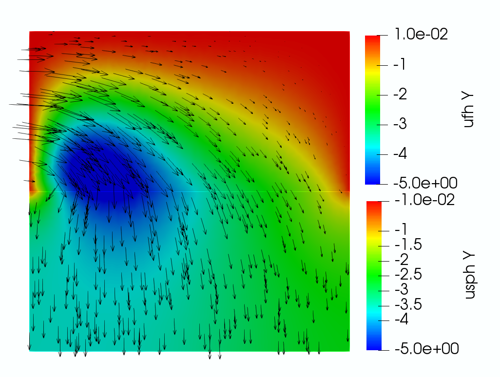
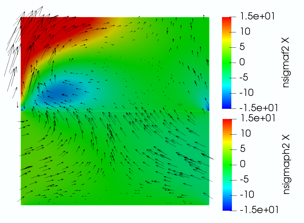
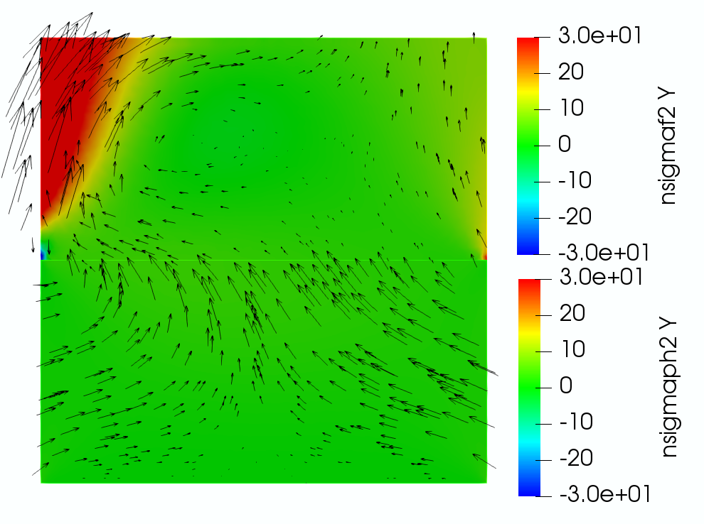
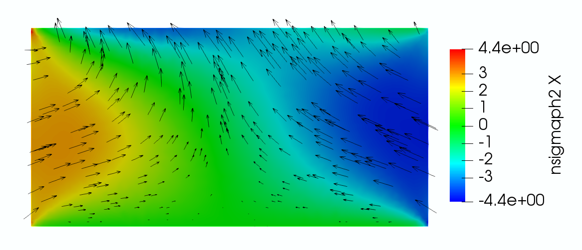
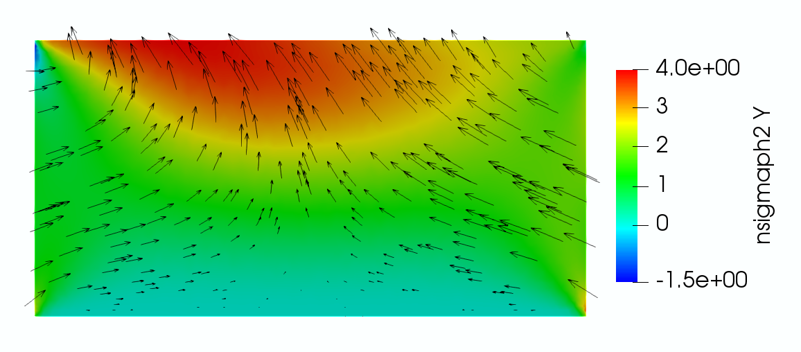
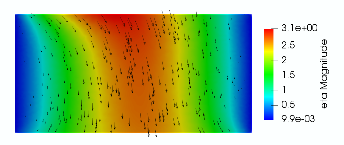
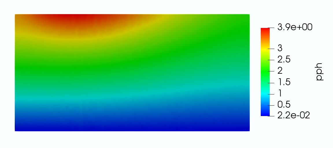
Figure 1: Example 2, Case 1, $\mathbf{K}=\mathbf{I}$, $s_{0}=1$, $\lambda_{p}=1$, $\mu_{p}=1$. Computed solution at final time $T=3$. Top left: velocities $\mathbf{u}_{f}$ and $\mathbf{u}_{p}+\partial_{t}{\bm{\eta}}_{p}$ (arrows), $\mathbf{u}_{f,2}$ and $\mathbf{u}_{p,2}+\partial_{t}{\bm{\eta}}_{p,2}$ (color). Top middle and right: stresses $-({\bm{\sigma}}_{f,12},{\bm{\sigma}}_{f,22})^{\mathrm{t}}$ and $-({\bm{\sigma}}_{p,12},{\bm{\sigma}}_{p,22})^{\mathrm{t}}$ (arrows); top middle: $-{\bm{\sigma}}_{f,12}$ and $-{\bm{\sigma}}_{p,12}$ (color); top right: $-{\bm{\sigma}}_{f,22}$ and $-{\bm{\sigma}}_{p,22}$ (color). Middle: poroelastic stress $-({\bm{\sigma}}_{p,12},{\bm{\sigma}}_{p,22})^{\mathrm{t}}$ (arrows); middle left: $-{\bm{\sigma}}_{p,12}$ (color); middle right: $-{\bm{\sigma}}_{p,22}$ (color). Bottom left: displacement ${\bm{\eta}}_{p}$ (arrows), $|{\bm{\eta}}_{p}|$ (color). Bottom right: Darcy pressure $p_{p}$.

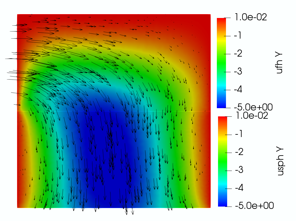
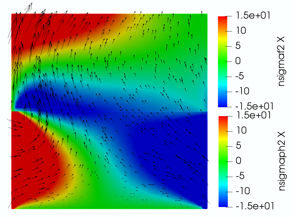
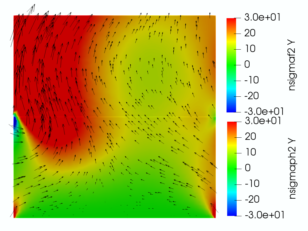
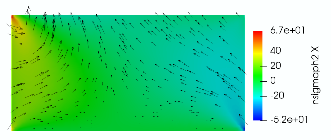
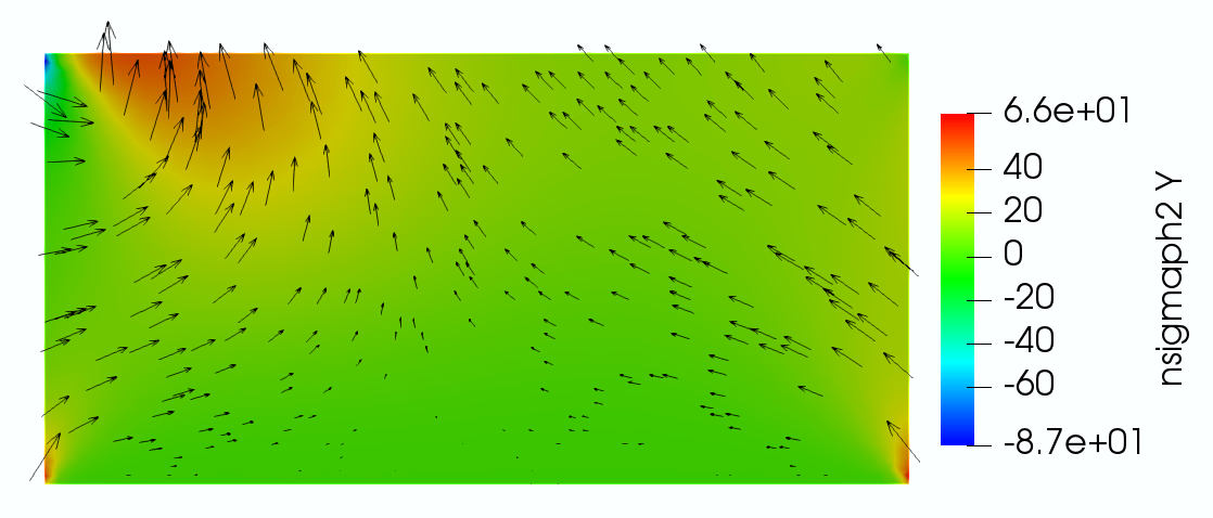
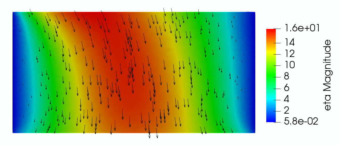
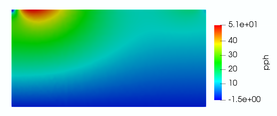
Figure 2: Example 2, Case 2, $\mathbf{K}=10^{-4}\times\mathbf{I}$, $s_{0}=10^{-4}$, $\lambda_{p}=10^{6}$, $\mu_{p}=1$. Computed solution at final time $T=3$. Top left: velocities $\mathbf{u}_{f}$ and $\mathbf{u}_{p}+\partial_{t}{\bm{\eta}}_{p}$ (arrows), $\mathbf{u}_{f,2}$ and $\mathbf{u}_{p,2}+\partial_{t}{\bm{\eta}}_{p,2}$ (color). Top middle and right: stresses $-({\bm{\sigma}}_{f,12},{\bm{\sigma}}_{f,22})^{\mathrm{t}}$ and $-({\bm{\sigma}}_{p,12},{\bm{\sigma}}_{p,22})^{\mathrm{t}}$ (arrows); top middle: $-{\bm{\sigma}}_{f,12}$ and $-{\bm{\sigma}}_{p,12}$ (color); top right: $-{\bm{\sigma}}_{f,22}$ and $-{\bm{\sigma}}_{p,22}$ (color). Middle: poroelastic stress $-({\bm{\sigma}}_{p,12},{\bm{\sigma}}_{p,22})^{\mathrm{t}}$ (arrows); middle left: $-{\bm{\sigma}}_{p,12}$ (color); middle right: $-{\bm{\sigma}}_{p,22}$ (color). Bottom left: displacement ${\bm{\eta}}_{p}$ (arrows), $|{\bm{\eta}}_{p}|$ (color). Bottom right: Darcy pressure $p_{p}$.

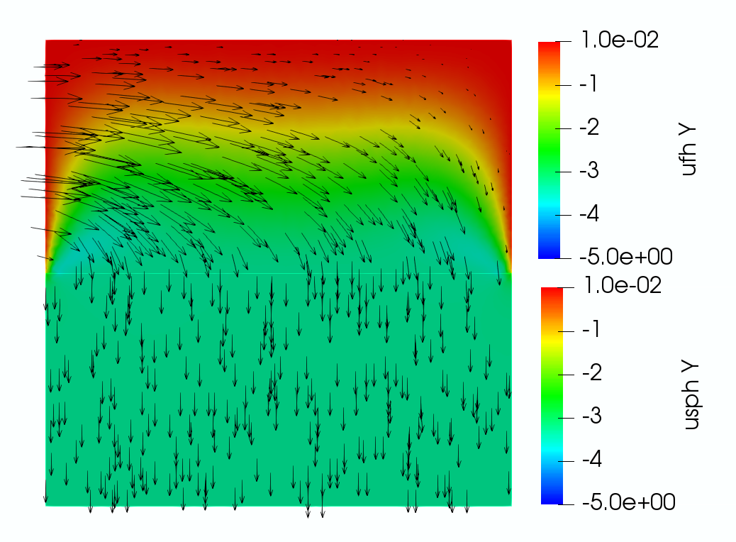
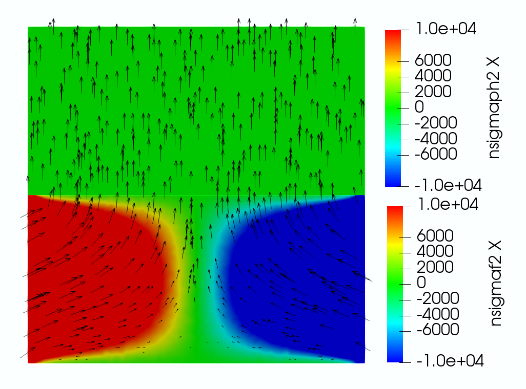
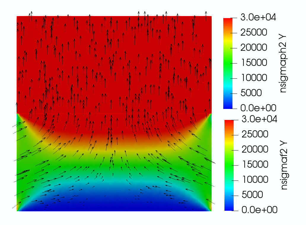
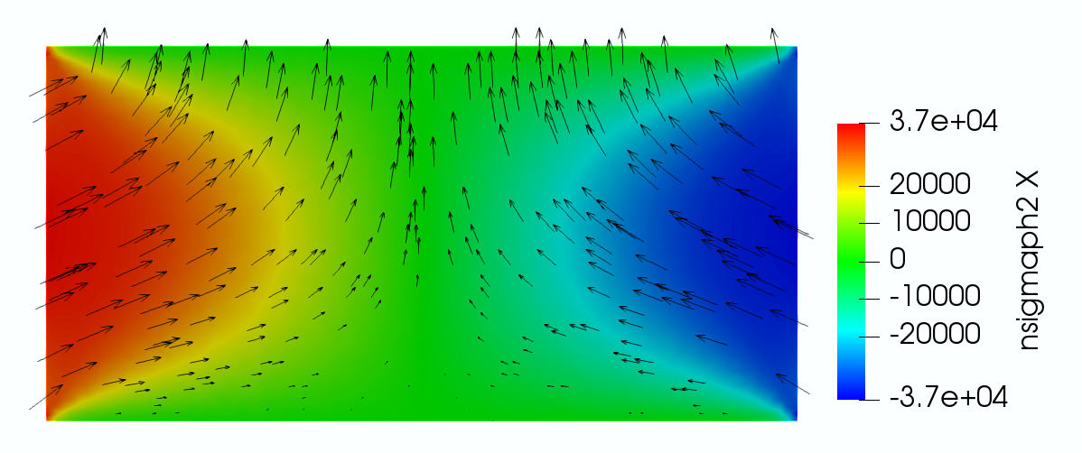
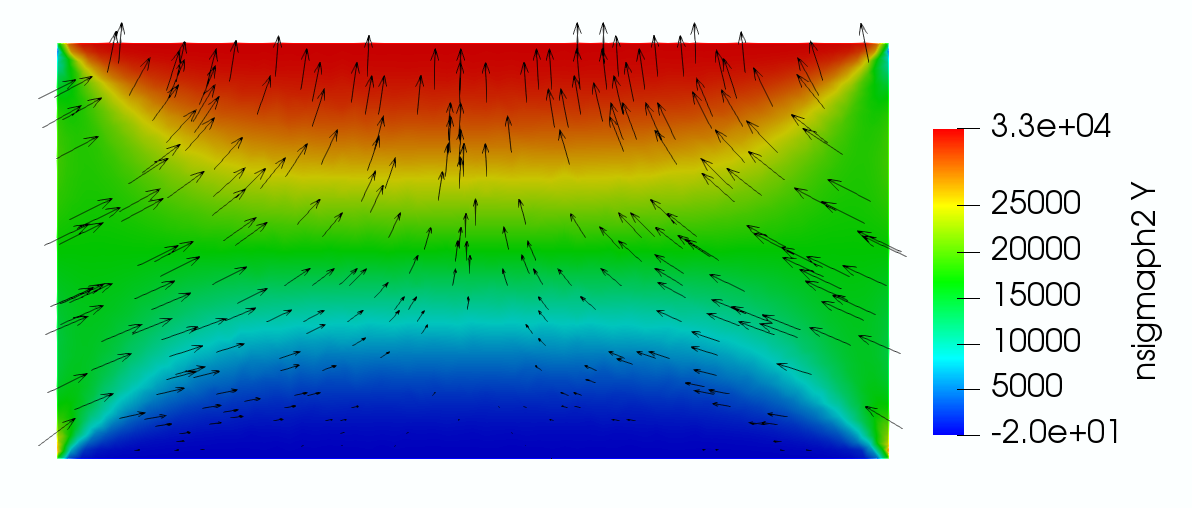
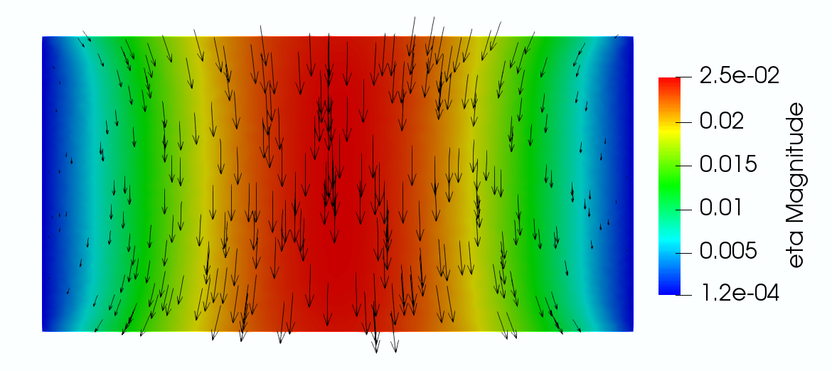
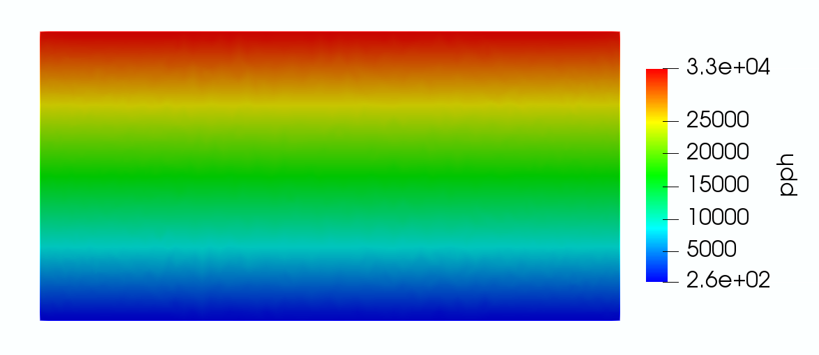
Figure 3: Example 2, Case 3, $\mathbf{K}=10^{-4}\times\mathbf{I}$, $s_{0}=10^{-4}$, $\lambda_{p}=10^{6}$, $\mu_{p}=10^{6}$. Computed solution at final time $T=3$. Top left: velocities $\mathbf{u}_{f}$ and $\mathbf{u}_{p}+\partial_{t}{\bm{\eta}}_{p}$ (arrows), $\mathbf{u}_{f,2}$ and $\mathbf{u}_{p,2}+\partial_{t}{\bm{\eta}}_{p,2}$ (color). Top middle and right: stresses $-({\bm{\sigma}}_{f,12},{\bm{\sigma}}_{f,22})^{\mathrm{t}}$ and $-({\bm{\sigma}}_{p,12},{\bm{\sigma}}_{p,22})^{\mathrm{t}}$ (arrows); top middle: $-{\bm{\sigma}}_{f,12}$ and $-{\bm{\sigma}}_{p,12}$ (color); top right: $-{\bm{\sigma}}_{f,22}$ and $-{\bm{\sigma}}_{p,22}$ (color). Middle: poroelastic stress $-({\bm{\sigma}}_{p,12},{\bm{\sigma}}_{p,22})^{\mathrm{t}}$ (arrows); middle left: $-{\bm{\sigma}}_{p,12}$ (color); middle right: $-{\bm{\sigma}}_{p,22}$ (color). Bottom left: displacement ${\bm{\eta}}_{p}$ (arrows), $|{\bm{\eta}}_{p}|$ (color). Bottom right: Darcy pressure $p_{p}$.

In Case 2 we test the model for a problem that exhibits both locking regimes for poroelasticity: 1) small permeability and storativity and 2) almost incompressible material [53]. In particular, we take $\mathbf{K}=10^{-4}\times\mathbf{I}$ and $s_{0}=10^{-4}$. Furthermore, the choice $\lambda_{p}=10^{6}$, $\mu_{p}=1$ results in Poisson’s ratio $\nu=0.4999995$. The computed solution does not exhibit locking or oscillations. The behavior is qualitatively similar to Case 1, with larger fluid and poroelastic stresses and a Darcy pressure gradient.

In Case 3, the Lamé coefficient $\mu_{p}$ is increased from $1$ to $10^{6}$, resulting in a much stiffer poroelastic medium, which is typical in subsurface flow applications. The solution is again free of locking effects or oscillations, but it differs significantly from Case 2, including three orders of magnitude larger stresses and Darcy pressure, as well as smaller displacement and Darcy velocity.

9 Conclusions

In this paper we developed and analyzed a new mixed elasticity formulation for the Stokes–Biot problem, as well as its mixed finite element approximation. We consider a five-field Biot formulation based on a weakly symmetric stress–displacement–rotation elasticity formulation and a mixed velocity–pressure Darcy formulation. The classical velocity–pressure formulation is used for the Stokes system. Suitable Lagrange multipliers are introduced to enforce weakly the balance of force, slip with friction, and continuity of normal flux on the interface. The advantages of the resulting mixed finite element method, compared to previous works, include local momentum conservation, accurate stress with continuous normal component, and robustness with respect to the physical parameters. In particular, the numerical results indicate locking-free and oscillation-free behavior in the regimes of small storativity and permeability, as well as for almost incompressible media.

References

- [1] I. Ambartsumyan, V. J. Ervin, T. Nguyen, and I. Yotov. A nonlinear Stokes-Biot model for the interaction of a non-Newtonian fluid with poroelastic media. ESAIM Math. Model. Numer. Anal., 53(6):1915–1955, 2019.
- [2] I. Ambartsumyan, E. Khattatov, T. Nguyen, and I. Yotov. Flow and transport in fractured poroelastic media. GEM Int. J. Geomath., 10(1):1–34, 2019.
- [3] I. Ambartsumyan, E. Khattatov, J. M. Nordbotten, and I. Yotov. A multipoint stress mixed finite element method for elasticity on simplicial grids. SIAM J. Numer. Anal., 58(1):630–656, 2020.
- [4] I. Ambartsumyan, E. Khattatov, J. M. Nordbotten, and I. Yotov. A multipoint stress mixed finite element method for elasticity on quadrilateral grids. Numer. Methods Partial Differential Equations, 37(3):1886–1915, 2021.
- [5] I. Ambartsumyan, E. Khattatov, and I. Yotov. A coupled multipoint stress–multipoint flux mixed finite element method for the Biot system of poroelasticity. Comput. Methods Appl. Mech. Engrg., 372:113407, 2020.
- [6] I. Ambartsumyan, E. Khattatov, I. Yotov, and P. Zunino. Simulation of flow in fractured poroelastic media: a comparison of different discretization approaches. In Finite difference methods, theory and applications, volume 9045 of Lecture Notes in Comput. Sci., pages 3–14. Springer, Cham, 2015.
- [7] I. Ambartsumyan, E. Khattatov, I. Yotov, and P. Zunino. A Lagrange multiplier method for a Stokes-Biot fluid-poroelastic structure interaction model. Numer. Math., 140(2):513–553, 2018.
- [8] D. Arnold and J. Lee. Mixed methods for elastodynamics with weak symmetry. SIAM J. Numer. Anal., 52(6):2743–2769, 2014.
- [9] D. N. Arnold, G. Awanou, and W. Qiu. Mixed finite elements for elasticity on quadrilateral meshes. Adv. Comput. Math., 41:553–572, 2015.
- [10] D. N. Arnold, R. S. Falk, and R. Winther. Mixed finite element methods for linear elasticity with weakly imposed symmetry. Math. Comp., 76(260):1699–1723, 2007.
- [11] S. Badia, A. Quaini, and A. Quarteroni. Coupling Biot and Navier-Stokes equations for modelling fluid-poroelastic media interaction. J. Comput. Phys., 228(21):7986–8014, 2009.
- [12] Y. Bazilevs, K. Takizawa, and T. E. Tezduyar. Computational fluid-structure interaction: methods and applications. John Wiley & Sons, 2013.
- [13] G. S. Beavers and D. D. Joseph. Boundary conditions at a naturally impermeable wall. J. Fluid. Mech, 30:197–207, 1967.
- [14] E. A. Bergkamp, C. V. Verhoosel, J. J. C. Remmers, and D. M. J. Smeulders. A staggered finite element procedure for the coupled Stokes-Biot system with fluid entry resistance. Comput. Geosci., 24(4):1497–1522, 2020.
- [15] M. Biot. General theory of three-dimensional consolidation. J. Appl. Phys., 12:155–164, 1941.
- [16] D. Boffi, F. Brezzi, L. F. Demkowicz, R. G. Durán, R. S. Falk, and M. Fortin. Mixed finite elements, compatibility conditions, and applications, volume 1939 of Lecture Notes in Mathematics. Springer-Verlag, Berlin; Fondazione C.I.M.E., Florence, 2008.
- [17] F. Brezzi and M. Fortin. Mixed and hybrid finite element methods, volume 15 of Springer Series in Computational Mathematics. Springer-Verlag, New York, 1991.
- [18] M. Bukač, I. Yotov, R. Zakerzadeh, and P. Zunino. Effects of poroelasticity on fluid-structure interaction in arteries: a computational sensitivity study. In Modeling the heart and the circulatory system, volume 14 of MS&A. Model. Simul. Appl., pages 197–220. Springer, Cham, 2015.
- [19] M. Bukač, I. Yotov, R. Zakerzadeh, and P. Zunino. Partitioning strategies for the interaction of a fluid with a poroelastic material based on a Nitsche’s coupling approach. Comput. Methods Appl. Mech. Engrg., 292:138–170, 2015.
- [20] M. Bukač, I. Yotov, and P. Zunino. An operator splitting approach for the interaction between a fluid and a multilayered poroelastic structure. Numer. Methods Partial Differential Equations, 31(4):1054–1100, 2015.
- [21] M. Bukač, I. Yotov, and P. Zunino. Dimensional model reduction for flow through fractures in poroelastic media. ESAIM Math. Model. Numer. Anal., 51(4):1429–1471, 2017.
- [22] H.-J. Bungartz and M. Schäfer. Fluid-structure interaction: modelling, simulation, optimisation, volume 53. Springer Science & Business Media, 2006.
- [23] A. Cesmelioglu and P. Chidyagwai. Numerical analysis of the coupling of free fluid with a poroelastic material. Numer. Methods Partial Differential Equations, 36(3):463–494, 2020.
- [24] A. Cesmelioglu, H. Lee, A. Quaini, K. Wang, and S.-Y. Yi. Optimization-based decoupling algorithms for a fluid-poroelastic system. In Topics in numerical partial differential equations and scientific computing, volume 160 of IMA Vol. Math. Appl., pages 79–98. Springer, New York, 2016.
- [25] S. Cesmelioglu. Analysis of the coupled Navier-Stokes/Biot problem. J. Math. Anal. Appl., 456(2):970–991, 2017.
- [26] P. Ciarlet. The Finite Element Method for Elliptic Problems. Studies in Mathematics and its Applications, Vol. 4. North-Holland Publishing Co., Amsterdam-New York-Oxford, 1978.
- [27] T. Davis. Algorithm 832: UMFPACK V4.3 - an unsymmetric-pattern multifrontal method. ACM Trans. Math. Software, 30(2):196–199, 2004.
- [28] M. Discacciati, E. Miglio, and A. Quarteroni. Mathematical and numerical models for coupling surface and groundwater flows. Appl. Numer. Math., 43(1-2):57–74, 2002.
- [29] H. C. Elman, D. J. Silvester, and A. J. Wathen. Finite elements and fast iterative solvers: with applications in incompressible fluid dynamics. Oxford University Press, 2014.
- [30] V. J. Ervin, E. W. Jenkins, and S. Sun. Coupled generalized nonlinear Stokes flow with flow through a porous medium. SIAM J. Numer. Anal., 47(2):929–952, 2009.
- [31] M. Fernández. Incremental displacement-correction schemes for the explicit coupling of a thin structure with an incompressible fluid. Comptes Rendus Math., 349(7):473–477, 2011.
- [32] G. P. Galdi and R. Rannacher, editors. Fundamental trends in fluid-structure interaction, volume 1 of Contemporary Challenges in Mathematical Fluid Dynamics and Its Applications. World Scientific Publishing Co. Pte. Ltd., Hackensack, NJ, 2010.
- [33] J. Galvis and M. Sarkis. Non-matching mortar discretization analysis for the coupling Stokes-Darcy equations. Electron. Trans. Numer. Anal., 26:350–384, 2007.
- [34] G. Gatica, A. Márquez, R. Oyarzúa, and R. Rebolledo. Analysis of an augmented fully-mixed approach for the coupling of quasi-newtonian fluids and porous media. Comput. Methods Appl. Mech. Engrg., 270:76–112, 2014.
- [35] G. Gatica, S. Meddahi, and R. Oyarzúa. A conforming mixed finite-element method for the coupling of fluid flow with porous media flow. IMA J. Numer. Anal., 29(1):86–108, 2009.
- [36] F. Hecht. New development in FreeFem++. J. Numer. Math., 20(3-4):251–265, 2012.
- [37] M. Jayadharan, E. Khattatov, and I. Yotov. Domain decomposition methods for mixed finite element discretizations of the Biot system of poroelasticity. Comput. Geosci., 2021, https://doi.org/10.1007/s10596-021-10091-w.
- [38] E. Khattatov and I. Yotov. Domain decomposition and multiscale mortar mixed finite element methods for linear elasticity with weak stress symmetry. ESAIM Math. Model. Numer. Anal., 53(6):2081–2108, 2019.
- [39] H. Kunwar, H. Lee, and K. Seelman. Second-order time discretization for a coupled quasi-Newtonian fluid-poroelastic system. Internat. J. Numer. Methods Fluids, 92(7):687–702, 2020.
- [40] W. J. Layton, F. Schieweck, and I. Yotov. Coupling fluid flow with porous media flow. SIAM J. Numer. Anal., 40(6):2195–2218, 2002.
- [41] J. Lee. Robust error analysis of coupled mixed methods for Biot’s consolidation model. J. Sci. Comput., 69(2):610–632, 2016.
- [42] V. Martin, J. Jaffré, and J. E. Roberts. Modeling fractures and barriers as interfaces for flow in porous media. SIAM J. Sci. Comput., 26:1667–1691, 2005.
- [43] T. Richter. Fluid-structure Interactions: Models, Analysis and Finite Elements, volume 118. Springer, 2017.
- [44] B. Riviere and I. Yotov. Locally conservative coupling of Stokes and Darcy flows. SIAM J. Numer. Anal., 42(5):1959–1977, 2005.
- [45] P. G. Saffman. On the boundary condition at the surface of a porous media. Stud. Appl. Math., 2:93–101, 1971.
- [46] R. E. Showalter. Monotone Operators in Banach Space and Nonlinear Partial Differential Equations. Mathematical Surveys and Monographs, 49. American Mathematical Society, Providence, RI, 1997.
- [47] R. E. Showalter. Poroelastic filtration coupled to Stokes flow. Control theory of partial differential equations. Lect. Notes Pure Appl. Math., 242, Chapman & Hall/CRC, Boca Raton, FL, pages 229–241, 2005.
- [48] R. E. Showalter. Nonlinear degenerate evolution equations in mixed formulation. SIAM J. Math. Anal., 42(5):2114–2131, 2010.
- [49] D. Vassilev, C. Wang, and I. Yotov. Domain decomposition for coupled Stokes and Darcy flows. Comput. Methods Appl. Mech. Engrg., 268:264–283, 2014.
- [50] J. Wen and Y. He. A strongly conservative finite element method for the coupled Stokes-Biot model. Comput. Math. Appl., 80(5):1421–1442, 2020.
- [51] H. K. Wilfrid. Nonconforming finite element methods for a Stokes/Biot fluid–poroelastic structure interaction model. Results Appl. Math., 7:100127, 2020.
- [52] S.-Y. Yi. Convergence analysis of a new mixed finite element method for Biot’s consolidation model. Numer. Meth. Partial. Differ. Equ., 30(4):1189–1210, 2014.
- [53] S.-Y. Yi. A study of two modes of locking in poroelasticity. SIAM J. Numer. Anal., 55(4):1915–1936, 2017.