The clustered selected-internal Steiner tree problem

Abstract

Given a complete graph $G=(V,E)$, with nonnegative edge costs, two subsets $R\subset V$ and $R^{\prime}\subset R$, a partition $\mathcal{R}=\{R_{1},R_{2},\ldots,R_{k}\}$ of $R$, $R_{i}\cap R_{j}=\phi$, $i\neq j$ and $\mathcal{R}^{\prime}=\{R^{\prime}_{1},R^{\prime}_{2},\ldots,R^{\prime}_{k}\}$ of $R^{\prime}$, $R^{\prime}_{i}\subset R_{i}$, a clustered Steiner tree is a tree $T$ of $G$ that spans all vertices in $R$ such that $T$ can be cut into $k$ subtrees $T_{i}$ by removing $k-1$ edges and each subtree $T_{i}$ spanning all vertices in $R_{i}$, $1\leq i\leq k$. The cost of a clustered Steiner tree is defined to be the sum of the costs of all its edges. A clustered selected-internal Steiner tree of $G$ is a clustered Steiner tree for $R$ if all vertices in $R^{\prime}_{i}$ are internal vertices of $T_{i}$, $1\leq i\leq k$. The clustered selected-internal Steiner tree problem is concerned with the determination of a clustered selected-internal Steiner tree $T$ for $R$ and $R^{\prime}$ in $G$ with minimum cost. In this paper, we present the first known approximation algorithm with performance ratio $(\rho+4)$ for the clustered selected-internal Steiner tree problem, where $\rho$ is the best-known performance ratio for the Steiner tree problem.

(xxxxxxxxxx)

1 Introduction

Given an undirected graph $G=(V,E)$, a subset $R\subseteq V$ of vertices, and a nonnegative edge cost function, a Steiner tree is used to find a tree in $G$ that spans all vertices in $R$. The given vertices $R$ are usually referred to as terminals and other vertices $V\setminus R$ as Steiner vertices. The cost of a Steiner tree is defined to be the sum of the costs of all its edges. The Steiner tree problem is concerned with the determination of a Steiner tree for $R$ in $G$ with minimum cost [8, 13, 14, 22]. The Steiner tree problem had been showed to be NP-Complete [15] and MAX SNP-hard [3]. Hence, many approximation algorithms had been designed for the Steiner tree problem [2, 4, 5, 19, 20, 27, 28, 33, 34]. Moreover, The Steiner tree problem had many significant applications in network routing, VLSI design, and phylogenetic tree reconstruction [6, 8, 12, 13, 14, 17, 22, 29, 31].

Motivated by the applications of the facility allocation in the (sensor) network and engineering change orders (ECO) in VLSI design, Hsieh and Yang [21] proposed a variant of the Steiner tree problem, called the selected-internal Steiner tree problem. Given a complete undirected graph $G=(V,E)$, a nonnegetive cost function on edges, and two subsets $R\subseteq V$ and $R^{\prime}\subset R$, a Steiner tree for $R$ in $G$ is a selected-internal Steiner tree if all terminals in $R^{\prime}$ are internal vertices of this Steiner tree. The selected-internal Steiner tree problem (SISTP for short) is concerned with the determination of a selected-internal Steiner tree for $R$ and $R^{\prime}$ in $G$ with minimum cost [21, 25]. For the SISTP, without loss of generality, we assume $|R\setminus R^{\prime}|\geq 2$ for the SISTP, otherwise the solution of SISTP may not exist. Then Hsieh and Yang [21] showed that the SISTP is NP-complete and MAX SNP-hard. They also proposed a $2\rho$-approximation algorithm for the SISTP on metric graphs (i.e., a complete graph and the lengths of edges satisfy the triangle inequality), where $\rho$ is the best-known performance ratio for the Steiner tree problem whose performance ratio is $\ln{4}+\epsilon\approx 1.39$ [5]. Li et al. [25] improved the performance ratio to $(\rho+1)$ for the SISTP.

Although the SISTP is defined by a group of vertices (terminals), some applications of computer and transportation network routing are considered in more than one group of vertices [1, 9, 11, 18, 24, 32]. Chisman [9] presented a variant of the traveling salesman problem [10, 16], called as the clustered traveling salesman problem. Wu and Lin [32] proposed another variant of the Steiner tree problem, called as the clustered Steiner tree problem. Given a complete graph $G=(V,E)$, with a nonnegetive cost function on edges, a subset $R\subset V$, and a partition $\mathcal{R}=\{R_{1},R_{2},\ldots,R_{k}\}$ of $R$, $R_{i}\cap R_{j}=\phi$, $i\neq j$, a clustered Steiner tree is a tree $T$ of $G$ that spans all vertices in $R$ such that $T$ can be cut into $k$ subtrees $T_{i}$ by removing $k-1$ edges and each subtree $T_{i}$ spanning all vertices in $R_{i}$, $1\leq i\leq k$. In other word, all the vertices in the same cluster ($R_{i}$) are clustered together in $T$. Each subtree $T_{i}$ is called as a local tree of $T$. The cost of a clustered Steiner tree is defined to be the sum of the costs of all its edges. The local cost of a clustered Steiner tree is the sum of the costs of all its edges in all its local trees. Then the inter-cluster cost of a clustered Steiner tree is the sum of the costs of remaining edges. The clustered Steiner tree problem (CSTP for short) is concerned with the determination of a clustered Steiner tree $T$ for $R$ in $G$ with minimum cost. Wu and Lin [32] showed that the CSTP is NP-complete and proposed a $(\rho+2)$-approximation algorithm for the CSTP on metric graphs. In this paper, we presented a variant of the SISTP and the CSTP, called as the clustered selected-internal Steiner tree problem. Given a complete graph $G=(V,E)$, with a nonnegetive cost function on edges, two subsets $R\subset V$ and $R^{\prime}\subset R$, a partition $\mathcal{R}=\{R_{1},R_{2},\ldots,R_{k}\}$ of $R$, $R_{i}\cap R_{j}=\phi$, $i\neq j$, and $\mathcal{R}^{\prime}=\{R^{\prime}_{1},R^{\prime}_{2},\ldots,R^{\prime}_{k}\}$ of $R^{\prime}$, $R^{\prime}_{i}\subset R_{i}$, a clustered selected-internal Steiner tree of $G$ is a clustered Steiner tree for $R$ if all vertices in $R^{\prime}_{i}$ are internal vertices of $T_{i}$, $1\leq i\leq k$. The clustered selected-internal Steiner tree problem (CSISTP for short) is concerned with the determination of a clustered selected-internal Steiner tree $T$ for $R$ and $R^{\prime}$ in $G$ with minimum cost. It is not hard to see the CSISTP is NP-hard, since the SISTP is its special versions when $k=1$. A Possible application of the CSISTP is to combine the applications of the SISTP and the CSTP in the following scenarios. Suppose there is a group of $|R|$ hosts (servers) in a computer network. A multicast tree is about building a tree to connect the group such that data can be transmitted to the group. In some network resource allocation strategies, some specified hosts (servers) in the group must act as transmitters and the others need not have this restriction [21]. Hence, transmitters are represented by the internal vertices of the multicast tree. The cost of an edge of the multicast tree represents the transmission distance, building or routing costs between two hosts in the network. Hence, a multicast tree in a network whose some specified servers in the group must be transmitters can be modeled by the SISTP [21]. Then, for some communication networks, sometimes the edges are divided into two levels: inter-cluster or intra-cluster, possibly with different costs, qualities, and capacities. After the multicast tree is constructed, the communications between hosts in the same cluster should be routed locally rather than globally for the sake of capacity consideration or the simpleness of routing protocols [32]. If all local topologies are given [32]. The purpose is to design the inter-cluster topology, as well as the possible insertion of local Steiner vertices without violating their topologies. These reasons caused us to build a multicast tree which satisfies the definition of the CSTP and the SISTP, simultaneously.

In this paper, we design the first known approximation algorithm with performance ratio of $(\rho+4)$ for the CSISTP on metric graphs. The rest of this paper is organized as follows. In Section 2, we describe our $(\rho+4)$-approximation algorithm to solve the CSISTP. Finally, we give the concluding remarks in Section 3.

2 A $(\rho+4)$-Approximation Algorithm for the CSISTP

Formally, we list the definition of the CSISTP as follows.

Definition 2.1.

For a complete graph $G=(V,E)$, a subset $R\subset V$, a partition $\mathcal{R}=\{R_{1},R_{2},\ldots,R_{k}\}$ of $R$, $R_{i}\cap R_{j}=\phi$, $i\neq j$, a clustered Steiner tree is a tree $T$ of $G$ that spans all vertices in $R$ such that $T$ can be cut into $k$ subtrees $T_{i}$ by removing $k-1$ edges and each subtree $T_{i}$ spanning all vertices in $R_{i}$, $1\leq i\leq k$.

CSTP

(Clustered Steiner Tree Problem)

Instance:

A complete graph $G=(V,E)$ with a cost function $c:E\rightarrow\mathbb{R}_{\geq 0}$ on the edges, a subset $R\subset V$, a partition $\mathcal{R}=\{R_{1},R_{2},\ldots,R_{k}\}$ of $R$, $R_{i}\cap R_{j}=\phi$, $i\neq j$.

Problem:

Find a clustered Steiner tree $T$ for $R$ in $G$ such that the sum of the costs of all its edges in $T$ is minimized.

Definition 2.2.

For a complete graph $G=(V,E)$, two subsets $R\subset V$ and $R^{\prime}\subset R$, a partition $\mathcal{R}=\{R_{1},R_{2},\ldots,R_{k}\}$ of $R$, $R_{i}\cap R_{j}=\phi$, $i\neq j$, and $\mathcal{R}^{\prime}=\{R^{\prime}_{1},R^{\prime}_{2},\ldots,R^{\prime}_{k}\}$ of $R^{\prime}$, each $R^{\prime}_{i}\subset R_{i}$. A clustered selected-internal Steiner tree of $G$ is a clustered Steiner tree for $R$ if all vertices in $R^{\prime}_{i}$ are internal vertices of $T_{i}$, $1\leq i\leq k$.

CSISTP

(Clustered Selected-Internal Steiner Tree Problem)

Instance:

A complete graph $G=(V,E)$ with a cost function $c:E\rightarrow\mathbb{R}_{\geq 0}$ on the edges, two subsets $R\subset V$ and $R^{\prime}\subset R$, a partition $\mathcal{R}=\{R_{1},R_{2},\ldots,R_{k}\}$ of $R$, $R_{i}\cap R_{j}=\phi$, $i\neq j$, and $\mathcal{R}^{\prime}=\{R^{\prime}_{1},R^{\prime}_{2},\ldots,R^{\prime}_{k}\}$ of $R^{\prime}$, each $R^{\prime}_{i}\subset R_{i}$.

Problem:

Find a clustered selected-internal Steiner tree $T$ for $R$ and $R^{\prime}$ in $G$ such that the sum of the costs of all its edges in $T$ is minimized..

For a subgraph $T$ of $G$, the cost of a tree $T=(V_{T},E_{T})$, denoted by $c(T)$, is the sum of the costs of all its edges in $T$, that is, $c(T)=\sum_{e\in E_{T}}c(e)$. The following examples illustrate the CSTP, SISTP and CSISTP, respectively. Consider the instance shown in Fig. 1, in which the graph $G=(V,E)$, $R=\{A,B,C,D,E,F\}$, and $R^{\prime}=\{C,F\}$. An optimal solution $T_{b}$ of $G$ for the CSTP with $k=3$ when $R_{1}=\{A,B\},R_{2}=\{C,D,E\},R_{3}=\{F\}$ is shown in Fig. 2, in which $c(T_{b})=23$. An optimal solution $T_{c}$ of $G$ for the SISTP is shown in Fig. 3, in which $c(T_{c})=22$. An optimal solution $T_{d}$ of $G$ for the CSISTP with $k=2$ when $R_{1}=\{A,B,F\},R_{2}=\{C,D,E\}$, $R_{1}^{\prime}=\{F\},R_{2}^{\prime}=\{C\}$ is shown in Fig. 4, in which $c(T_{d})=25$.

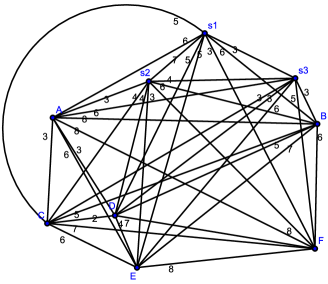
Figure 1: An instance: A complete graph $G=(V,E)$, $R=\{A,B,C,D,E,F\}$, $R^{\prime}=\{C,F\}$.

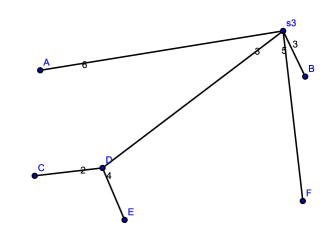
Figure 2: The optimal solution $T_{b}$ when $R_{1}=\{A,B\},R_{2}=\{C,D,E\},R_{3}=\{F\}$ for the CSTP. (Note that $c(T_{b})=23$).

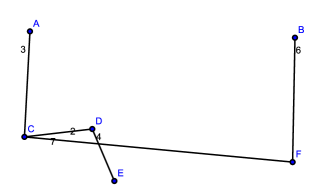
Figure 3: The optimal solution $T_{c}$ for the SISTP. (Note that $c(T_{c})=22$).

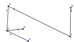
Figure 4: The optimal solution $T_{d}$ when $R_{1}=\{A,B,F\},R_{2}=\{C,D,E\}$, $R_{1}^{\prime}=\{F\},R_{2}^{\prime}=\{C\}$ for the CSISTP. (Note that $c(T_{d})=25$).

Definition 2.3.

For a cluster Steiner tree $T$ spanning $R$, the local tree of $T_{i}$ on $T$ is the minimal subtree of $T$ that spans all vertices in $R_{i}$, $1\leq i\leq k$.

In this section, we present a $(\rho+4)$-approximation algorithm for the CSISTP, whose cost function is metric. For a complete graph $G=(V,E)$, let $c(u,v)$ denote the cost of a edge $(u,v)$, for the two vertices $u,v\in V$. For a vertex subset $S$, let $G[S]$ denote the subgraph of $G$ induced by $S$. A minimum spanning tree (MST for short) [10, 26] of $G[S]$ is concerned with the determination of a tree spanning all verteices in $S$ with minimum cost of $G[S]$. We let $A_{mst}(G[S])$ be the algorithm to find a minimum spanning tree of $G[S]$. For a graph $H=(V_{H},E_{H})$, the contraction of an edge $(u,v)$ is to replace the two vertices $u$ and $v$ with a new vertex $w$, and then the edge cost is assigned to $c(w,x)=\min{\{c(u,x),c(v,x)\}}$ for any other vertex $x$. For a subgraph $S=(V_{S},E_{S})$ in $H$, the contraction of $S$ in $H$ means to contract all the edges of $E_{S}$ in an arbitrary order, and the resulting graph is denoted by $H/S$. For convenience, we also use $H/S$ to $H/H[S]$ when $S$ is a vertex subset. Finally, we let $G/R$ denote the graph resulted from contracting every $R_{i}\in R$, $1\leq i\leq k$, i.e., each cluster $R_{i}$ is concentrated into a vertex [32].

Definition 2.4.

For a graph $G=(V,E)$, a Hamiltonian path of $V$ is a path that visits each vertex in $V$ exactly once.

Definition 2.5.

A graph $G=(V,E)$ is Hamiltonian-connected if for every pair of vertices $u$ and $v$, the two vertices can be connected by a Hamiltonian path from $u$ to $v$.

For any clustered Steiner tree $T$ and each its local tree $T_{i}$ of $R_{i}$, Wu and Lin [32] showed $T$ can be transformed into a clustered Steiner tree $\widehat{T}$ such that each local tree $\widehat{T}_{i}$ of $\widehat{T}$ is a Hamiltonian Path of $R_{i}$. By Wu and Lin’s algorithm [32], for any clustered Steiner tree $T$, if the vertex $r$ in $R_{i}$ is an internal vertex in $T_{i}$, the vertex $r$ is also an internal vertex in $\widehat{T}_{i}$. Hence, Wu and Lin’s algorithm [32] also satisfies any clustered selected-internal Steiner tree for $R$ and $R^{\prime}$ in $G$, i.e., each vertex in $R^{\prime}_{i}$ is also an internal vertex in $\widehat{T}_{i}$.

Definition 2.6.

[32] For a clustered Steiner tree $T$ for $R$, the inter-cluster tree of $T$ is that the contraction of all its local trees becomes in a tree, denoted by $T/R$.

For any clustered Steiner tree $T$ for $R$ and its local tree $T_{i}$, $1\leq i\leq k$, the next three lemmas come from [32].

Lemma 2.7.

Each local tree $T_{i}$ is replaced with a Hamiltonian path $\widehat{T}_{i}$ of $R_{i}$ and each vertex in $R^{\prime}_{i}$ is a internal vertex of $\widehat{T}_{i}$, $1\leq i\leq k$. We have $c(\widehat{T}_{i})\leq 2c(T_{i})$.

Lemma 2.8.

For each inter-cluster tree $\widehat{T}/R$ of $\widehat{T}$, we have $c(\widehat{T}/R)\leq c(T)$.

Since each clustered Steiner tree $T$ satisfies the Lemma 2.7 and Lemma 2.8, we have next Lemma.

Lemma 2.9.

Let $T_{opt}$ be the optimal solution for the CSTP. There exists a clustered Steiner tree $\widehat{T}$ such that each local tree $\widehat{T}_{i}$ of $\widehat{T}$ is a Hamiltonian Path of $R_{i}$ and each vertex in $R^{\prime}_{i}$ is a internal vertex of $\widehat{T}_{i}$ that $c(\widehat{T}/R)\leq c(T_{opt})$.

Given a connected graph $G=(V,E)$, the cube of $G$, denoted by $G^{3}=(V,E_{G^{3}})$, is the graph with the same vertex set as $G$ and any edge $(u,v)$ in $E_{G^{3}}$ if and only if there exists a path between the two vertices $u$ and $v$ in $G$ and the number of edges in the path is at most three. Independently, Sekanina [30] and Karaganis [23] proved that the cube of every connected graph with at least three vertices is Hamiltonian-connected. We let $A_{h}(G,u,v)$ be the algorithm for finding a Hamiltonian path between the two vertices $u$ and $v$ in the $G^{3}$ by Karaganis’ proof [23], whose time-complexity is $O(|V|^{2})$. See Appendixm or Chen [7] for more details of this algorithm. For a tree $T=(V_{T},E_{T})$ and $(u,w),(w,v)\in E_{T}$, we define the shortcut between $u$ and $v$ is to replace edges $(u,w)$ and $(w,v)$ with $(u,v)$.

Lemma 2.10.

For every tree $T=(V_{T},E_{T})$ of $G$, if $T^{h}=(V_{T},E_{T^{h}})$ is the output of Hamiltonian-path of $V_{T}$ by $A_{h}(T,u,v)$, we have $c(T^{h})\leq 2c(T)$ by the triangle inequality with doubling the tree edges $E_{T}$ and then traversal shortcuts between the adjacent vertices in $T^{h}$.

Now, we describe the $(\rho+4)$-approximation algorithm for the CSISTP. First, for each $R_{i}$, we use Algorithm $A_{mst}(G[R_{i}])$ to find a MST $T^{s}_{i}$ of $G[R_{i}]$, $1\leq i\leq k$. Next, select any two vertices $u$ and $v$ in $R_{i}\setminus R^{\prime}_{i}$ (Note that $|R_{i}\setminus R^{\prime}_{i}|\geq 2$). Then we use $A_{h}(T^{s}_{i},u,v)$ to find a Hamiltonian path $T^{h}_{i}$ between the two vertices $u$ and $v$ in the cube of $T^{s}_{i}$. By Lemma 2.10, we have $c(T^{h}_{i})\leq 2c(T^{s}_{i})$, $1\leq i\leq k$. Moreover. we construct $G/R$ and let $\widetilde{R}=\{r_{i}|1\leq i\leq k\}$, where $r_{i}$ is the vertex resulted from the contraction of $R_{i}$. For a graph $G=(V,E)$ with a subset $R\subseteq V$, let $\mathcal{A}_{stp}(G,R)$ be the $\rho$-approximation algorithm to solve the Steiner tree problem for $R$ in $G$. Furthermore, we use $\mathcal{A}_{stp}(G/R,\widetilde{R})$ to find an inter-cluster tree that spans all vertices in $\widetilde{R}$. Finally, replace each $r_{i}$ with $T^{h}_{i}$ to obtain a clustered Steiner tree (also a clustered selected-internal Steiner tree).

For clarification, we describe the approximation algorithm for the CSISTP as follows.

Algorithm APX

Input:

A complete graph $G=(V,E)$ with a nonnegetive cost function $c$ on edges, two subsets $R\subset V$ and $R^{\prime}\subset R$, a partition $\mathcal{R}=\{R_{1},R_{2},\ldots,R_{k}\}$ of $R$, $R_{i}\cap R_{j}=\phi$, $i\neq j$, and $\mathcal{R}^{\prime}=\{R^{\prime}_{1},R^{\prime}_{2},\ldots,R^{\prime}_{k}\}$ of $R^{\prime}$, $R^{\prime}_{i}\subset R_{i}$, where the cost function is metric.

Output:

A clustered selected-internal Steiner tree $\mathcal{T}$ for $R$ and $R^{\prime}$ in $G$.

1.

For each $R_{i}$, use Algorithm $A_{mst}(G[R_{i}])$ [10, 26] to find a MST $T^{s}_{i}$ of $G[R_{i}]$, $1\leq i\leq k$.

2.

For each $T^{s}_{i}$, select any two vertices $u$ and $v$ in $R_{i}\setminus R^{\prime}_{i}$, and then use Algorithm $A_{h}(T^{s}_{i},u,v)$ to find a Hamiltonian path $T^{h}_{i}$ between the two vertices $u$ and $v$ in the cube of $T^{s}_{i}$.

3.

Construct $G/R$ and let $\widetilde{R}=\{r_{i}|1\leq i\leq k\}$, where $r_{i}$ is the vertex resulted from the contraction of $R_{i}$.

4.

Use Algorithm $\mathcal{A}_{stp}(G/R,\widetilde{R})$ to find the inter-cluster tree that spans all vertices in $\widetilde{R}$.

5.

Replace each $r_{i}$ with $T^{h}_{i}$ to obtain a clustered selected-internal Steiner tree $\mathcal{T}$.

The result of this section is summarized in the following theorem.

Theorem 2.11.

Algorithm APX is a $(\rho+4)$-approximation algorithm for the CSISTP.

Proof 2.12.

We first analyze the time-complexity of Algorithm APX as follows. For each $R_{i}$, use Prim’s Algorithm [10, 26] to find a MST for $G[R_{i}]$ takes $O(|R_{i}|^{2})$ time. Hence, step 1 runs $O(|R|^{2})$ time. Also, step 2 can take $O(|R|^{2})$ time [23]. Step 3 and step 5 take $O(|V|^{2})$ and $O(|V|)$ time, respectively. Hence, the time-complexity of Algorithm APX is dominated by the cost of the step 3 for running the $\rho$-approximation algorithm for the STP.

Next, we prove the performance ratio of Algorithm APX. Let $T_{opt}$ be the optimal solution for the CSISTP for $R$ and $R^{\prime}$ in $G$ and $T^{o}_{i}$ is its local tree of $R_{i}$, $1\leq i\leq k$. We also let $\widehat{T}$ be a tree satisfying Lemma 2.7–2.9. For each local tree $T^{h}_{i}$, we have $c(T^{h}_{i})\leq 2c(T^{s}_{i})$ by Lemma 2.10. Since each $T^{s}_{i}$ is a MST of $G[R_{i}]$, by Lemma 2.7, we have $c(T^{s}_{i})\leq c(\widehat{T}_{i})\leq 2c(T^{o}_{i})$. Then the cost of $\widehat{T}/R$ is greater than or equal to the cost of the optimal solution for the Steiner tree problem for $\widetilde{R}$ in the graph $G/R$. Step 5 runs a $\rho$-approximation algorithm to solve the Steiner tree problem for $\widetilde{R}$ in the graph $G/R$. Hence, $c(\mathcal{T}/R)\leq\rho c(\widehat{T}/R)\leq\rho c(T_{opt})$ by Lemma 2.8–2.9. Finally, we have

$$c(\mathcal{T})=\sum_{i=1}^{k}c(T^{h}_{i})+c(\mathcal{T}/R) \leq 2\sum_{i=1}^{k}c(T^{s}_{i})+\rho c(T_{opt})$$

$$\leq 4\sum_{i=1}^{k}c(T^{o}_{i})+\rho c(T_{opt})\leq(\rho+4)c(T_{opt}),$$

and the theorem is proved.

3 Conclusion

In this paper, we have investigated the CSISTP. Then we have proposed an approximation algorithm with performance ratio of $(\rho+4)$ for the CSISTP on metric graphs. For future research, improving the performance ratio for the CSISTP is an immediate direction.

Appendix A Appendix

Karaganis [23] proved that the cube of a connected graph $G$ with at least three vertices is Hamiltonian-connected, i.e., there exists a Hamiltonian path between any two vertices. In this proof, Karaganis let $T$ be a spanning tree of $G$ and construct a Hamiltonian path between any two vertices $v_{a}$ and $v_{b}$ in $T^{3}$ recursively, in which $T^{3}$ is the cube of $T$. We list the algorithm, denoted by $A_{h}(T,v_{a},v_{b})$, as follows.

Algorithm $A_{h}(T,v_{a},v_{b})$

Input:

A tree $T=(V_{T},E_{T})$ with two vertices $v_{a}$ and $v_{b}$ of $T$.

Output:

A Hamiltonian path $T^{h}$ between $v_{a}$ and $v_{b}$ in $T^{3}$.

Repeat the following steps until the condition $|V_{T}|=1$ holds.

1.

If $v_{a}$ and $v_{b}$ are not adjacent then

1.1.

Find a path $P=(v_{a},v_{1},v_{2},\ldots,v_{b})$ between $v_{a}$ and $v_{b}$ in $T$.

1.2.

Cut the edge $(v_{a},v_{1})$ in $T$ such that $T$ be separated into two trees, say $T_{v_{a}}$ and $T_{v_{b}}$ respectively, containing $v_{a}$ and $v_{b}$.

1.3.

If the number of the vertex of $T_{v_{a}}$ is one then let $v_{a^{\prime}}$ be $v_{a}$ else let $v_{a^{\prime}}$ be a vertex adjacent to $v_{a}$ in $T_{v_{a}}$.

1.4.

Let $v_{b^{\prime}}$ be the vertex $v_{1}$ in $T_{v_{b}}$.

   

Else

1.5.

Cut the edge $(v_{a},v_{b})$ in $T$ such that $T$ be separated into two trees, say $T_{v_{a}}$ and $T_{v_{b}}$ respectively, containing $v_{a}$ and $v_{b}$.

1.6.

If the number of the vertex of $T_{v_{a}}$ is one then let $v_{a^{\prime}}$ be $v_{a}$ else let $v_{a^{\prime}}$ be a vertex adjacent to $v_{a}$ in $T_{v_{a}}$.

1.7.

If the number of the vertex of $T_{v_{b}}$ is one then let $v_{b^{\prime}}$ be $v_{b}$ else let $v_{b^{\prime}}$ be a vertex adjacent to $v_{b}$ in $T_{v_{b}}$.

2.

Call $A_{h}(T_{v_{a}},v_{a},v_{a^{\prime}})$ to find a Hamiltonian path $P_{v_{a}}$ between $v_{a}$ and $v_{a^{\prime}}$ in $T_{v_{a}}^{3}$.

3.

Call $A_{h}(T_{v_{b}},v_{b^{\prime}},v_{b})$ to find a Hamiltonian path $P_{v_{b}}$ between $v_{b^{\prime}}$ and $v_{b}$ in $T_{v_{b}}^{3}$.

4.

Connect $P_{v_{a}}$ and $P_{v_{b}}$ by the edge $(v_{a^{\prime}},v_{b^{\prime}})$.

After running $A_{h}(T,v_{a},v_{b})$, Karaganis [23] proved that there exists a Hamiltonian path between the two vertices $v_{a}$ and $v_{b}$ in $T^{3}$. By the triangle inequality and traversal shortcuts between the adjacent vertices in $T^{h}$, it is clear that $c(T^{h})\leq 2c(T)$. Let F($|V_{T}|$) be the time complexity of $A_{h}(T,v_{a},v_{b})$ on a tree $T$ with $|V_{T}|$ vertices. Then we can express $F(|V_{T}|)$ recursively as a recurrence relation : $F(|V_{T}|)=O(|V_{T}|)+F(|V_{T_{v_{a}}}|)+F(|V_{T_{v_{b}}}|)$ and the solution of $F(|V_{T}|)$ is $O(|V_{T}|^{2})$ time.

References

- [1] X. Bao and Z. Liu, An improved approximation algorithm for the clustered traveling salesman problem, Information Processing Letters 112 (2012) 908–910.
- [2] P. Berman and V. Ramaiyer, Improved approximations for the Steiner tree problem, Journal of Algorithms 17 (1994) 381–408.
- [3] M. Bern and P. Plassmann, The Steiner tree problem with edge lengths 1 and 2, Information Processing Letters 32 (1989) 171–176.
- [4] A. Borchers and D.Z. Du, The -Steiner ratio in graphs, SIAM Journal on Computing 26 (1997) 857–869.
- [5] J. Byrka, F. Grandoni, T. Rothvos and L. Sanita, Steiner Tree Approximation via Iterative Randomized Rounding, Journal of the Association for Computing Machinery 60 (2013) 6.
- [6] A. Caldwell, A. Kahng, S. Mantik, I. Markov and A. Zelikovsky, On wirelength estimations for row-based placement, IEEE Transactions on Computer-Aided Design of Integrated Circuits and Systems 18(9) (1999) 1265–1278.
- [7] Y.H. Chen, The bottleneck selected-internal and partial terminal Steiner tree problems, Networks 68(4) (2016) 331–339.
- [8] X. Cheng and D.Z. Du, Steiner Trees in Industry (Kluwer Academic Publishers, Dordrecht, Netherlands, 2001).
- [9] J.A. Chisman, The clustered traveling salesman problem, Computers & Operations Research (1975) 115–119.
- [10] T.H. Cormen, C.E. Leiserson, R.L. Rivest and C. Stein, Introduction to Algorithm, 3rd edition (MIT Press, Cambridge, 2009).
- [11] C. Ding, Y. Cheng and M. He, Two-level genetic algorithm for clustered traveling salesman problem with application in large-scale TSPs, Tsinghua Science & Technology 12 (2007) 459–465.
- [12] L.M.A. Drummond and M. Santos, A distributed dual ascent algorithm for Steiner problems in multicast routing, Networks 53 (2009) 170–183.
- [13] D.Z. Du, J.M. Smith and J.H. Rubinstein, Advance in Steiner Tree (Kluwer Academic Publishers, Dordrecht, Netherlands, 2000).
- [14] D.Z. Du and X. Hu, Steiner tree problems in computer communication networks (World Scientific Publishing Company, 2008).
- [15] M. Garey, R. Graham and D. Johnson, The complexity of computing Steiner minimal trees, SIAM Journal on Applied Mathematics 32 (1977) 835–859.
- [16] A Golovnev, Approximating asymmetric tsp in exponential time, International Journal of Foundations of Computer Science bf 25 (01) (2014) 89–99.
- [17] D. Graur and W.H. Li, Fundamentals of Molecular Evolution, second edition (Sinauer Publishers, Sunderland, MA, 2000).
- [18] N. Guttmann-beck, R. Hassin, S. Khuller and B. Raghavachari, Approximation algorithms with bounded performance guarantees for the clustered traveling salesman problem, Algorithmica 28 (2000) 422–437.
- [19] S. Hougardy and H.J. Promel, A 1.598 approximation algorithm for the Steiner tree problem in graphs, Proceedings of the 10th Annual ACM–SIAM Symposium on Discrete Algorithms (SODA) (Baltimore, USA, 1999), pp. 448–453.
- [20] S. Hougardy and S. Kirchner, Lower bounds for the relative greedy algorithm for approximating Steiner trees, Networks 47 (2006) 111–115.
- [21] S.Y. Hsieh and S.C. Yang, Approximating the selected-internal Steiner tree, Theoretical Computer Science 381 (2007) 288–291.
- [22] F.K. Hwang, D.S. Richards and P. Winter, The Steiner Tree Problem, In: Annuals of Discrete Mathematics, Vol. 53 (Elsevier Science Publishers, Amsterdam, 1992).
- [23] J.J. Karaganis, On the cube of a graph, Canadian Mathematical Bulletin 11 (1968) 295–296.
- [24] G. Laporte, J.Y. Potvin and F. Quilleret, A Tabu search heuristic using genetic diversification for the clustered traveling salesman problem, Journal of Heuristics 2 (1995) 187–200.
- [25] X. Li, F. Zou, Y. Huang, D. Kim and W. Wu, A better constant-factor approximation for selected-internal Steiner minimum tree, Algorithmica 56 (2010) 333–341.
- [26] R.C. Prim, Shortest connection networks And some generalizations, Bell System Technical Journal 36 (1957) 1389–1401.
- [27] H.J. Prommel and A. Steger, A new approximation algorithm for the Steiner tree problem with performance ratio 5/3, Journal of Algorithms 36 (2000) 89–101.
- [28] G. Robins and A. Zelikovsky, Tighter bounds for graph Steiner tree approximation, SIAM Journal on Discrete Mathematics 19 (2005) 122–134.
- [29] P. Saikia and S. Karmakar, Distributed approximation algorithms for Steiner tree in the congested clique, International Journal of Foundations of Computer Science 31 (07) (2020) 941–968.
- [30] M. Sekanina, On an ordering of the set of vertices of a connected graph, Publications of the Faculty of Science, University of Brno 412 (1960) 137–141.
- [31] P. Winter, Steiner problem in networks: A survey, Networks 17 (1987) 129–167.
- [32] B.Y. Wu and C.W. Lee, On the clustered Steiner tree problem, Journal of Combinatorial Optimization 30 (2015) 370–386.
- [33] A. Zelikovsky, An 11/6-approximation algorithm for the network Steiner problem, Algorithmica 9 (1993) 463–470.
- [34] A. Zelikovsky, A faster approximation algorithm for the Steiner tree problem in graphs, Information Processing Letters 46 (1993) 79–83.