Systolic Computing on GPUs for Productive Performance

Abstract.

We propose a language and compiler to productively build high-performance software systolic arrays that run on GPUs. Based on a rigorous mathematical foundation (uniform recurrence equations and space-time transform), our language has a high abstraction level and covers a wide range of applications. A programmer specifies a projection of a dataflow compute onto a linear systolic array, while leaving the detailed implementation of the projection to a compiler; the compiler implements the specified projection and maps the linear systolic array to the SIMD execution units and vector registers of GPUs. In this way, both productivity and performance are achieved in the same time. This approach neatly combines loop transformations, data shuffling, and vector register allocation into a single framework. Meanwhile, many other optimizations can be applied as well; the compiler composes the optimizations together to generate efficient code.

We implemented the approach on Intel GPUs. This is the first system that allows productive construction of systolic arrays on GPUs. We allow multiple projections, arbitrary projection directions and linear schedules, which can express most, if not all, systolic arrays in practice. Experiments with 1- and 2-D convolution on an Intel GEN9.5 GPU have demonstrated the generality of the approach, and its productivity in expressing various systolic designs for finding the best candidate. Although our systolic arrays are purely software running on generic SIMD hardware, compared with the GPU’s specialized, hardware samplers that perform the same convolutions, some of our best designs are up to 59% faster. Overall, this approach holds promise for productive high-performance computing on GPUs.

1. Introduction

All modern GPUs achieve performance via hardware multi-threading and SIMD (single-instruction multiple-data), and an efficient memory hierarchy (Fatahalian and Houston, 2008). The mainstream programming languages such as CUDA and OpenCL essentially expose an SIMT (single-instruction multiple-threads) programming interface, and rely on an underlying compiler to transparently map a wrap of threads to SIMD execution units. If data need to be exchanged among threads in the same wrap, programmers have to write explicit shuffle instructions (NVidia, 2020).

This paper proposes a new programming style that programs GPUs as building software systolic arrays. Systolic arrays have been extensively studied since 1978 (Kung and Leiserson, 1978), and shown an abundance of practice-oriented applications, mainly in fields dominated by iterative procedures (Zehendner, 2007), e.g. image and signal processing, matrix arithmetic, non-numeric applications, relational database (H.T. Kung, 1982; Kurzak et al., 2013; Wei et al., 2017; Intel, 2019a; Kung et al., 1987; Intel, 2017; Hughey, 1991), and so on.

A systolic array is composed of many hardware PEs (Processing Elements) that have the same instructions and works rhythmically: every time step, the PEs typically read inputs from some neighbors, process the inputs, and forward the inputs or results to other neighbors. Therefore, systolic arrays can be viewed as “the combination of SIMD and the pipeline architectures characteristics” (Quinton, 1987), a fact that has been observed for a long time.

Based on this fact, we can build a systolic array on a GPU by mapping the PEs to the SIMD lanes of the GPU, and realizing the data forwarding using shuffle instructions among vector registers. This idea has been proposed as “software systolic array” by Chen et al., and demonstrated on stencils and convolution manually with competitive performance (Chen et al., 2019). Similar ideas can be found elsewhere. For examples, Pondemente, Luna and Alba used GPUs to build systolic arrays for a generic search algorithm (Alba and Vidal, 2012), Wang et al. implemented sequence alignment algorithms on GPUs in a systolic style without mentioning it (Wang et al., 2017). All these works were done on Nvidia GPUs in the CUDA language.

These state-of-art works, however, focus on specific workloads, and the systolic arrays were built in high programming skills. None of the works has pointed out a general, systematic solution how to build on GPUs arbitrary systolic arrays for the numerous workloads that are known to benefit from systolic algorithms. And they have not provided a productive tool for quickly building systolic arrays on GPUs, either.

In this paper, we present a language and compiler to productively build high-performance systolic arrays that run on GPUs. A programmer specifies a dataflow compute in uniform recurrence equations (UREs), and a projection of the compute onto a linear systolic array in a space-time transform. We allow multiple projections, arbitrary projection directions and linear schedules. Our approach has the following characteristics:

1. Generality.

   UREs and space-time transform are the theoretical foundation of most systolic arrays we can see in the real world. They are rigorously formulated in mathematics and have been extensively studied. By enabling them, our language and compiler are able to cover the wide range of applications to which numerous systolic arrays apply.

2. Productivity.

   Our language has a higher abstraction level than the popular, SIMT-based programming languages like CUDA and OpenCL. Both UREs and space-time transforms are succinct math: UREs are a functional notation of a compute, and space-time transforms are expressed by matrices.

   Our language separates concerns of programmers. For a compute, programmers write its functional notation (UREs) and its optimizations (space-time transforms, and other loop and data optimizations) separately.

   Our language is a specification language: programmers only specify optimizations, but leave their detailed implementation to a compiler; the compiler implements the optimizations, particularly, maps linear systolic arrays determined by the specified space-time transforms to the SIMD execution units and vector registers of GPUs. In this way, both productivity and performance are achieved in the same time.

3. Performance.

   A space-time transform neatly combines loop transformations, data shuffling, and vector register allocation together: it can transform a loop nest in a single shot with the combined effect of several loop transformations (like loop reordering, skewing and vectorization), allocation of minimum number of vector registers, and shuffling of the data in the registers.

   Meanwhile, many other optimizations can be applied as well. These optimizations include tiling, multi-threading, building a memory hierarchy with shared memory and registers, etc. The compiler composes the optimizations together to generate efficient code.

We prototyped a system for our approach on Intel GPUs (Intel, 2015). We leverage Susy (Lai et al., 2020), a system that enabled UREs and limited space-time transforms for FPGAs. Susy allows only a single projection, and the projection direction must follow a loop dimension. In our system, we break the limitations to allow multiple projections and arbitrary projection directions, and generate code for GPUs, which is essentially different from FPGAs, and necessitates substantial innovation. From the perspective of programming style, Susy for FPGAs is single-thread SIMD, while our language for GPUs is a mix of SIMT and SIMD. From the perspective of hardware architectures, FPGAs have on-chip memory but no hardware caches, have massive programmable logic resources and registers, while GPUs have shared memory, hardware caches, fixed execution units, and limited thread-private registers, and thus the compiler has to optimize very differently.

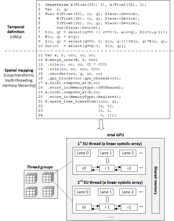
Figure 1. The overall flow.

Fig. 1 provides a high-level overview of our system. Programmers write a specification, which contains two parts: (1) a temporal definition, which is a functional definition of the compute to perform, in the form of UREs, and (2) a spatial mapping, which is optimizations to map the compute efficiently to a GPU. These optimizations transform loops (e.g. by loop tiling, reordering, space-time transform, etc.), enable multi-threading, and build a memory hierarchy. In more detail, the iteration space of a dataflow compute is cut into groups of software threads, and scheduled group by group to a GPU at runtime; every software thread is mapped to a hardware thread called Execution Unit (EU) thread. For brevity, we will use the term thread to refer to a software thread, and EU thread for its corresponding hardware thread.

Unlike a traditional thread, a thread here contains a linear systolic array, as specified by a space-time transform as part of the spatial mapping. The linear systolic array is realized by the SIMD function units and vector registers in a EU thread. More specifically, every lane of a SIMD function unit is a PE, and the PEs exchange data by shuffling the vector registers that contain the data. One may view a thread here as a wrap of threads in CUDA.

This is the first system that allows productive construction of systolic arrays on GPUs, to the best of our knowledge. We remark that although the current system targets only Intel GPUs, it is general and should be applicable to other GPUs as well.

We performed initial experiments with 1- and 2-dimensional convolution on an Intel Gen9.5 GPU, and compared the performance with the hardware samplers of the GPU performing the same convolutions. The experiments show that the approach is very general and flexible; various systolic designs of the convolutions can be expressed succinctly in 10-20 minutes, and thus programmers can quickly search for the best designs; the best designs are 14%-59% faster than the specialized hardware samplers, which is very encouraging since our systolic arrays are purely software on generic SIMD hardware. Overall, these initial results show that our approach holds promise for productive high-performance computing on GPUs.

2. Background

In this section, we briefly introduce necessary background knowledge. Throughout the paper, any vector is assumed to be a column vector, except pointed out otherwise.

2.1. Uniform Recurrence Equation

We follow Quinton’s definition of URE (Quinton, 1984) with slight generalization (Xue, 1992). A system of UREs are equations, each of which has the following form:

(1) $$V_{i}(\vec{z})=f(V_{1}(\vec{z}-\vec{e_{1}}),V_{2}(\vec{z}-\vec{e_{2}}),...,V_{p}(\vec{z}-\vec{e_{p})})$$

where $V_{1},V_{2},...,V_{p}$ are variables, $f$ is an arbitrary function, $\vec{z}$ is a (computation) point (i.e. an iteration) in an $n$-dimensional space, and point $\vec{z}$ reads variables $V_{1},V_{2},...,V_{p}$ from the previous points at constant distances of $\vec{e_{1}},\vec{e_{2}},...,\vec{e_{p}}$, respectively (We assume that there is only one dependence associated with one variable). In other words, the UREs represent an $n$-deep loop nest with a uniform dependence structure.

UREs are a functional way to express a computation so that any memory location $V_{i}(\vec{z})$ is written only once. This is called dynamic single-assignment (DSA) (Vanbroekhoven et al., 2007). The read-write relationship between computation points is explicit, which makes it easy for a compiler to analyze and parallelize the computation.

2.2. Space-time Transform

A space-time transform projects the computation points in an $n$-dimensional space to an $n-1$-dimensional space, and schedules the points to execute in temporal order. Following the notations of Chen and Kung (Chen and Kung, 1998), let $\vec{d}$ be a projection vector that projects the points to the $n-1$-dimensional space. In the $n-1$-dimensional space, the coordinates of the points are $n-1$-dimensional vectors, and can be viewed as linear combinations of the column vectors of a $(n-1)*n$ allocation matrix (also called projection matrix) $\mathbf{P}$. The projection vector is a normal vector of the $n-1$-dimensional space and thus there must be $\mathbf{P}\vec{d}=0$. Also let $\vec{s}$ be a scheduling vector representing the time scheduling. Then a point $\vec{z}$ in the original space is mapped to $\bigl{(}\begin{smallmatrix}\mathbf{P}\\ \vec{s}^{T}\end{smallmatrix}\bigr{)}\vec{z}=\bigl{(}\begin{smallmatrix}\mathbf{P}\vec{z}\\ \vec{s}^{T}\vec{z}\end{smallmatrix}\bigr{)}$. That is, point $\vec{z}$ in the original space is allocated to point $\mathbf{P}\vec{z}$ in the new space, and is scheduled to execute at time step $\vec{s}^{T}\vec{z}$. The points in the new space is what we referred to as PEs before. See Fig. 2 for an illustration.

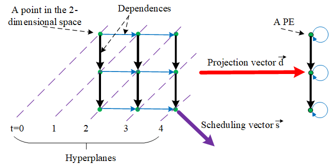
Figure 2. Illustrating the concept of space-time transform. Here 9 points in a 2-dimensional space are projected to run on 3 PEs in a 1-dimensional space. The dependences are projected accordingly.

A transform is valid if and only if the following conditions are satisfied (Chen and Kung, 1998):

• Data availability: $\vec{s}^{T}\vec{e}\geq 0$ for any dependence $\vec{e}$. $\vec{s}^{T}\vec{e}\neq 0$ for non-broadcast data.

• Processor availability: $\vec{s}^{T}\vec{d}>0$.

The first condition ensures that for any dependence (except read-after-read, or so-called broadcast), its source point has to be executed before its sink point. The second condition ensures that two computation points, if mapped to the same PE, do not execute at the same time.

Multiple projections can be applied to an $n$-dimensional space. They can be collectively expressed by a single space-time transform. Fig. 3 illustrates the concept with a 3-dimensional space projected to a 1-dimensional space after two projections. This example, however, can be generalized to arbitrary multiple projections. We leave the detailed theory to a literature (Chen and Kung, 1998).

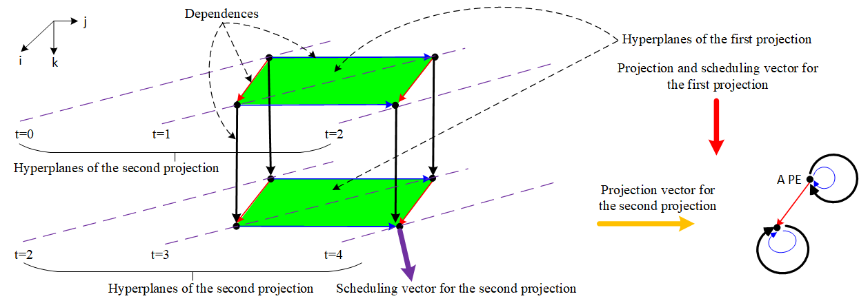
Figure 3. Illustration of multiple projection. In this example, there are 2 projections that project a 3-dimensional space $(i,j,k)$ into a 1-dimensional space. When expressing the two projections in a single space-time transform, one may find that the time schedule equals $i+j+2*k$; in other words, the scheduling vector $\vec{s}$ equals $\bigl{(}\begin{smallmatrix}1&1&2\end{smallmatrix}\bigr{)}^{T}$. One may also find that any compute point $(i,j,k)$ are mapped to a PE indexed by $i$, i.e. the allocation matrix equals $\bigl{(}\begin{smallmatrix}1&0&0\end{smallmatrix}\bigr{)}$.

3. Language and Programming Model

As we said, our language is a specification language for GPUs. Typically, a specification is written in our language following a specific pattern: a set of UREs expressing a temporal definition, followed by a spatial mapping. In the spatial mapping, all UREs are merged together as the body of the same loop nest; for this loop nest, loop tiling and reordering are usually performed first, so as to create a final shape of the loop nest; then some outermost loops are designated as the loops for scanning thread groups, and for scanning the threads in a group, respectively; after that, the input data are loaded either to shared memory (and then into registers automatically by the compiler), or to registers directly; finally, other loop optimizations are applied for performance; particularly, every thread is built into a systolic array by a space-time transform of the UREs. In our programming model, registers are private to threads.

Table 1 describes a minimal set of the language features. The space_time_transform primitive is the main feature this paper proposes. As said before, it is much more general than the same named feature in Susy (Lai et al., 2020), and internally targets GPUs instead of FPGAs. In a space-time transform, we allow only linear schedules, which is the most popularly used in practice. Thus this is not a real restriction in the real world.

Table 1. Primitives of our language.

Primitive	Description
Func F([return type, arguments, place])	Declare a function. The return type and arguments must be declared for a recurrence function. Place is where the function will be running, either CPU (i.e. Place::Host) or GPU (i.e. Place::Device). The default place is CPU.
F(arguments)=select(condition, value1 [, value2])	Define a function. The function returns value1 if condition is true, or value2 otherwise. If value2 is not specified, the function is undefined when condition is false.
F.merge_ures(G, H, ...)	Put the set of UREs F, G, H, ... as the body of the loop nest of function F.
F.tile(var, var${}_{\texttt{o}}$, var${}_{\texttt{i}}$, factor)	Tile the loop variable var of F into two new variables var${}_{\texttt{o}}$ and var${}_{\texttt{i}}$ with a factor of factor.
F.reorder(var1, var2, ..., var${}_{\texttt{n}}$)	Reorder the loop nest of function F according to the specified order (starting from the innermost level).
F.gpu_blocks(x, [y, [,z]])	The groups of threads are scanned by loop x (and y, z if specified).
F.gpu_threads(x, [y, [,z]])	The threads in a group are scanned by loop x (and y, z if specified).
F.in(G)	The call to F in function G.
F.compute_at(G, x)	Compute function F at loop level x of function G, which calls function F.
F.store_in(memory type)	Store the values of function F in a given type of memory, e.g. shared memory or registers.
F.space_time_transform(source loops,	Map the source loops of function F to the destination loops with the transform matrix.
destination loops, transform matrix	The loops are specified to start from the innermost level. The transform matrix is in the
[, reverse transform]	form of $\bigl{(}\begin{smallmatrix}\mathbf{P}\\ \vec{s}^{T}\end{smallmatrix}\bigr{)}$, where $\mathbf{P}$ and $\vec{s}$ are the allocation matrix and scheduling vector, respectively
[, SpaceTimeTransform::CheckTime])	(See Section 2).
	The reverse transform describes how to map from the destination loop variables after the transform back to the source variables before the transform. The reverse transform is optional when the transform matrix is unimodular, in which case the compiler can automatically compute the reverse transform.
	If SpaceTimeTransform::CheckTime is specified, the compiler generates an explicit check for each PE to execute only when its time steps come; otherwise, every PE always runs and the programmer needs ensure that does not affect correctness.

3.1. Illustrating the Language, Programming Model and IR Changes

Fig. 1 illustrates our language with a specific design for 1-D convolution. The mathematical definition of 1-D convolution is

(2) $$Z(c)=\sum\limits_{q}x(c+q)*w(q)$$

where $x$ is a sequence of input data, and $w$ is a short sequence of weights. At every position $c$ of the output sequence, the weight sequence multiplies with the corresponding input data, and generates one result $Z(c)$.

There are many systolic designs for convolution accelerators. According to Jo, Kim and Park (Jo et al., 2018), these designs can be classified based on the following ordered combinations of inputs, weights and partial sums:

An input or weight

• B: is Broadcast to all PEs,

• F: is Forwarded from one PE to another, or

• S: Stays in a PE,

and a partial sum is

• A: Aggregated from all PEs,

• M: Migrated from one PE to another, or

• S: Sedimented in a PE.

Fig. 4 illustrates one of the designs, namely SBM (Jo et al., 2018), in which the inputs stay in each PE, the weights are broadcast to all the PEs, and the partial sums migrate from a PE to another.

The top half of Fig. 1 contains a specification to express this design. The capitalized symbols in the example specification (and in the rest of the paper) like CC etc. represent static constants. In the temporal definition of the specification, Line 7-9 define the 1-D convolution according to Equation 2, but in a recurrent form. These recurrent equations can be intuitively derived by following the dataflow in Fig. 4. Line 10 defines an output function Out that takes a final value of Z after the corresponding recurrent computation is done. Function Out is not really a URE, but is treated so by the compiler to be simple. As we can see, the temporal definition of a compute is close to the original mathematical definition in Equation 2, and exposes the dataflow. This makes it easy for programmers to define the functionality of the compute and for the compiler to analyze dependences, which is an advantage of the programming model.

In the spatial mapping, Line 12 makes the UREs the body of the loop nest of function X. The compiler will build an intermediate representation (IR) for the loop nest like this:

⬇

for (c = 0; c < C; c++)

for (q = 0; q < Q; q++)

X(c,q) = select(q==0||c==C-1,x(c+q), X(c+1,q-1))

W(c,q) = w(q)

Z(c,q) = select(q==0, 0, Z(c,q-1))+X(c,q)*W(c,q)

Out(c) = select(q==Q-1, Z(c,q))

Then Line 13-15 split the outer loop twice into 3 loops, and reorder all the loops. Then Line 16 designates the outermost two loops for scanning thread groups and threads, respectively. Line 17-20 load the weights and inputs for each thread into shared memory and registers, respectively. Consequently, the loop nest becomes like this:

⬇

parallel for (oc=0; oc< C/CC/CCC; oc++) // Groups

parallel for (cc = 0; cc < CC; cc++) // Threads

if (oc == 0 && cc == 0)

allocate, and load weights into, shared memory

load weights from shared memory into registers

load inputs to be used into registers

for (q = 0; q < Q; q++)

for (ccc = 0; ccc < CCC; ccc++)

c = oc * CC * CCC + cc * CCC + ccc

X(c,q)=select(q==0||c==C-1,x(c+q),X(c+1,q-1))

W(c,q)=w(q)

Z(c,q)=select(q==0,0, Z(c,q-1))+X(c,q)*W(c,q)

Out(c)=select(q==Q-1, Z(c,q))

Line 21-24 express the systolic array determined by the projection shown in Fig. 4. The source loops ccc and q are mapped to a space loop s and a time loop t by a transform matrix $\bigl{(}\begin{smallmatrix}1&1\\ 0&1\end{smallmatrix}\bigr{)}$, which means that s = ccc + q and t = q. This is a unimodular matrix, and the compiler can automatically find the reverse transform. The compiler maps variable X, W, and Z to vector registers based on the transform matrix, and determines the sizes of the vector registers as Q + CCC -1. The compiler then replaces the references to the variables with references to the vector registers. Consequently, the two source loops ccc and q become like this:

⬇

vector<float, Q + CCC - 1> X, W, Z;

for (t = 0; t < Q; t++)

vectorize for (s = 0; s < Q + CCC - 1; s++)

q, ccc = t, s - t // Reverse transform

c = oc * CC * CCC + cc * CCC + ccc

X(s)=select(q==0||c==C-1,x(c+q),X(s))

W(s)=w(q)

Z(s)=select(q==0,0, Z(s-1))+X(s)*W(s)

Out(c)=select(q==Q-1, Z(s))

In the next section, we will explain in more detail how the above evolution of IR is realized by the compiler.

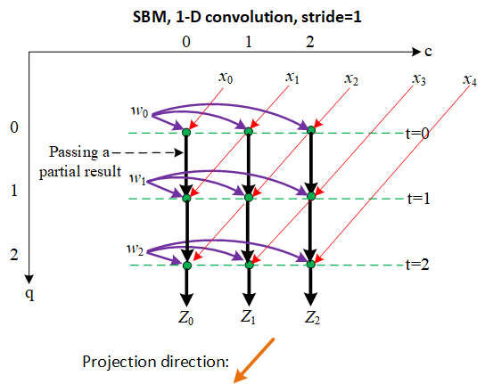
Figure 4. SBM systolic design for 1-D convolution.

4. Compiler

Fig. 5 shows our compilation flow. As we said, a specification contains a temporal definition and a spatial mapping. The compiler first records information according to the temporal definition, then based on that information, building an IR and transforming the IR according to the spatial mapping. This is a reactive compilation phase, in which the compiler performs only the specified optimizations. After that, the compiler enters a proactive compilation phase, where the compiler transparently optimize the IR. For example, the compiler may perform common sub-expression elimination to reduce the strength of computation, hoist loop invariant out of a loop, etc. Finally, the compiler generates code for the target GPU from the IR. Currently, we generate GPU code in the CM language (Intel, 2019b), which extends the standard C++ language with explicit SIMD support for GPUs to exploit data parallelism in applications. Particularly, our linear systolic arrays are realized in the CM language using matrices/vectors and SIMD operations that manipulate the matrices/vectors. Finally, we invoke the CM compiler to generate binaries for Intel GPUs.

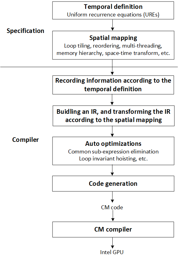
Figure 5. The compilation flow.

4.1. Space-time Transform

Here we describe the compiler implementation of space-time transform in more detail. As we said, no matter we project a loop nest once or multiple times, we can express the projection(s) in a single space-time transform. Let $\mathbf{P}$ be the allocation matrix, and $\vec{s}$ be the scheduling vector. To be simple but without losing generality, let us say the original IR is

⬇

1 $\mathbf{Code\ 1:\ Original\ IR\ Example}$

2int $V$[extents of $\vec{z}$];

3for loops of $\vec{z}$

4 $V[\vec{z}]=f(V[\vec{z}-\vec{e}])+g(\vec{z})$

where $V$ is a recurrent variable with a dependence distance vector $\vec{e}$, and $f$ and $g$ are arbitrary functions. Then in general, the compiler transforms the IR as follows:

⬇

1 $\mathbf{Code\ 2:\ Space-time\ Transformed\ IR\ Example}$

2int $V$[extent of $\mathbf{P}\vec{z}$][$\vec{s}^{T}\vec{e}$ + 1];

3for t = min($\vec{s}^{T}\vec{z}$); t <= max($\vec{s}^{T}\vec{z}$); t++

4 vectorize for each PE $\vec{x}\in\mathbf{P}\vec{z}$

5 $V[\vec{x}][1,2,...,\vec{s}^{T}\vec{e}$] = $V[\vec{x}][0,1,...,\vec{s}^{T}\vec{e}$-1]

6 $\vec{z}=h(\vec{x},t)$

7 if $\vec{z}$ is in the original iteration space

8 $V[\vec{x}][0]=f(V[\vec{x}+\mathbf{P}\vec{e}][\vec{s}^{T}\vec{e}])+g(\vec{z})$

Here h is a function that reverses the space-time transform so that from the current PE and time step, we can find the corresponding computation point in the original iteration space before the transform. If the transform matrix is unimodular, the compiler can compute its inverse matrix and that is the reverse transform h. Otherwise, the programmer must specify the reverse transform.

Note that in the above transformed IR, variable V in Line 2 must be a matrix: (1) $\mathbf{P}\vec{z}$ is the index of the PE on which the original point $\vec{z}$ is to run; the index is a scalar as the transform is for building a linear systolic array. Therefore, the first dimension of V, the extent (i.e. the upper bound) of $\mathbf{P}\vec{z}$ is the number of PEs in the linear systolic array, and is a static constant. (2) $\vec{s}^{T}\vec{e}$ is constant given that both $\vec{s}$ and $\vec{e}$ are static constant vectors. Therefore, the second dimension of V is also a static constant. A special case is that when $\vec{s}^{T}\vec{e}$ equals 0, variable V degenerates into a vector.

Therefore, in generating code for the transformed loop nest, the compiler maps variable V in Line 2 above to a matrix or vector. The dimensions of the matrix or vector are determined by the allocation matrix $\mathbf{P}$ and scheduling vector $\vec{s}$, in other words, space-time transform also performs register allocation for recurrent variables. In Line 5, every PE shuffles its own data. In Line 8, every PE gets an input from a neighbor PE at a constant space distance ($\mathbf{P}\vec{e}$) and a constant time distance ($\vec{s}^{T}\vec{e}$), performs some compute locally, and saves the results locally. Thus we can see that the entire body of the loop nest can be vectorized. That is why the loop in Line 4 is annotated as vectorized.

In short, the data type to generate is matrix or vector, and the operations are vectorized. Since the CM language is specialized in matrix/vector types and operations, we choose to generate CM code.

4.1.1. Optimized Code Generation for Special Cases

Above we have illustrated a space-time transformed IR in general. Here we discuss special cases for which we may reduce register usage and/or produce more compact code.

In the Code 1 (original IR example) above, we can see that a previous value of variable V, $V[\vec{z}-\vec{e}]$, is used, and it will never be used again. Therefore, the new value of variable V, $V[\vec{z}]$, can reuse the register assigned to the previous value. This is called register coalescing. Therefore, with some slight change to the code generation pattern, the compiler can generate the following code for space-time transform instead:

⬇

1 $\mathbf{Code\ 3:\ Space-time\ Transformed\ IR\ Example}$

2 $\mathbf{\ after\ Register\ Coalescing}$

3int $V$[extent of $\mathbf{P}\vec{z}$][$\vec{s}^{T}\vec{e}$];

4for t = min($\vec{s}^{T}\vec{z}$); t <= max($\vec{s}^{T}\vec{z}$); t++

5 vectorize for each PE $\vec{x}\in\mathbf{P}\vec{z}$

6 $\vec{z}=h(\vec{x},t)$

7 int $tmp$;

8 if $\vec{z}$ is in the original iteration space

9 $tmp=f(V[\vec{x}+\mathbf{P}\vec{e}][\vec{s}^{T}\vec{e}])+g(\vec{z})$

10 $V[\vec{x}][1,2,...,\vec{s}^{T}\vec{e}$ - 1] = $V[\vec{x}][0,1,...,\vec{s}^{T}\vec{e}$-2]

11 $V[\vec{x}][0]=tmp$

Note that the second dimension of V is now $\vec{s}^{T}\vec{e}$: 1 register is saved for each PE. Also, when $\vec{s}^{T}\vec{e}$ equals 1, Line 10 above (register shifting) can be removed. And if the programmer has not specified SpaceTimeTransform::CheckTime when using the space_time_transform() primitive, the above code can be further simplified:

⬇

1 $\mathbf{Code\ 4:\ Space-time\ Transformed\ IR\ Example\ with}$

2$\mathbf{\vec{s}^{T}\vec{e}=1,Register\ Coalescing,\ and\ without\ Checking}$

3int $V$[extent of $\mathbf{P}\vec{z}$];

4for t = min($\vec{s}^{T}\vec{z}$); t <= max($\vec{s}^{T}\vec{z}$); t++

5 vectorize for each PE $\vec{x}\in\mathbf{P}\vec{z}$

6 $\vec{z}=h(\vec{x},t)$

7 $V[\vec{x}]=f(V[\vec{x}+\mathbf{P}\vec{e}])+g(\vec{z})$

For example, for the specification shown at the top half of Fig. 1, one may find that all the variables can be register coalesced. Further, variable X and Z have a dependence with a distance $\vec{e}=\bigl{(}\begin{smallmatrix}-1\\ 1\end{smallmatrix}\bigr{)}$ and $\bigl{(}\begin{smallmatrix}0\\ 1\end{smallmatrix}\bigr{)}$, respectively. With the scheduling vector $\vec{s}=\bigl{(}\begin{smallmatrix}0&1\end{smallmatrix}\bigr{)}$, we have $\vec{s}^{T}\vec{e}=1$ for both dependences. Also, SpaceTimeTransform::CheckTime is not specified. Therefore, the above Code 4 style of code generation can be applied, which results in the transformed IR as shown at the end of Section 3.1.

5. Generality and Flexibility: with 1-D and 2-D Convolution as Examples

Our approach is based on UREs and space-time transforms. This makes our approach very general: UREs and space-time transforms are the theoretical foundation of most, if not all, systolic arrays. They have been extensively studied during the past several decades, and have been used to design numerous systolic arrays from various domains (H.T. Kung, 1982; Hughey, 1991; Quinton, 1987). They are also mathematically simple and rigorous.

This approach is also flexible: from one systolic design, often with slight changes in its UREs and/or transform matrix, a new systolic design can be created. This opens an avenue for exploring the systolic design space for the best designs.

In this section, we demonstrate the generality and flexibility of our approach with various designs of 1-D and 2-D convolution. We have shown a design, SBM, for 1-D convolution before in Fig. 4, and its UREs and space-time transform in the specificaiton in Fig. 1. Here we show several other designs for 1-D convolution in Table 2. Among them, BSM, FSM, BFS, and FFS were proposed by Jo, Kim and Park for an ASIC implementation by manually transforming dataflow graphs (Jo et al., 2018). Here we express the same designs, but use UREs and space-time transforms instead (See the descriptions in the table). The UREs and space-time transforms for each design can be used to replace those in the example specification in Fig. 1.

To further show the generality and flexibility, in Table 2, we also present a new design, FBS, for 1-D convolution, with a stride of 1 and 2, respectively.

All these designs for 1-D convolution involve only one projection. To demonstrate multiple projections, we also look at 2-D convolution, which is defined as below:

(3) $$Z(c,r)=\sum\limits_{q}\sum\limits_{p}x(c+q,r+p)*w(q,p)$$

Fig. 6 show the SBM design for 2-D convolution. Although it looks complicated, following the dataflow, we can easily figure out the UREs as follows:

⬇

X(c,p,q,r)=select(c==C-1||q=0,x(c+q,r+p),X(c+1,p,q-1,r))

W(c,p,q,r)=w(q,p)

Z(c,p,q,r)=select(p==0 && q==0, 0,

select(p==0,Z(c,p+P-1,q-1,r), Z(c,p-1,q,r)))

+ X(c,p,q,r) * W(c,p,q,r)

Out(c, r)=select(p==P-1 && q==Q-1, Z(c,p,q,r))

Following the two projection directions shown in the figure, we can easily figure out that the allocation matrix is $\bigl{(}\begin{smallmatrix}1&0&1\end{smallmatrix}\bigr{)}$, i.e. a computation point at (c, p, q) at any given r will be mapped to PE c + q.

Following the two scheduling directions shown in the figure, we can also easily figure out that the scheduling vector is $\bigl{(}\begin{smallmatrix}0&1&P\end{smallmatrix}\bigr{)}$.

As we can see, UREs and space-time transforms can easily express all these designs. The mathematics involved is intuitive, and should be comfortably mastered by common programmers. Besides, programmers can leverage the wealth of research fruits accumulated in the past several decades.

Table 2. Several other systolic designs for 1-D convolution.

X(c, q) = x(c + q) W(c, q) = select(c == 0, w(q), W(c - 1, q)) Z(c, q) = select(q == 0, 0, Z(c, q - 1)) + X(c,q)*W(c,q) Space-time transform: $\bigl{(}\begin{smallmatrix}s\\ t\end{smallmatrix}\bigr{)}=\bigl{(}\begin{smallmatrix}0&1\\ 1&1\end{smallmatrix}\bigr{)}*\bigl{(}\begin{smallmatrix}c\\ q\end{smallmatrix}\bigr{)}$	X(c, q) = select(c == 0 || q == Q - 1, x(c + q), X(c - 1, q + 1)) W(c, q) = select(c == 0, w(q), W(c - 1, q)) Z(c, q) = select(q == Q - 1, 0, Z(c, q + 1)) + X(c,q)*W(c,q) Space-time transform: $\bigl{(}\begin{smallmatrix}s\\ t\end{smallmatrix}\bigr{)}=\bigl{(}\begin{smallmatrix}0&1\\ 1&-1\end{smallmatrix}\bigr{)}*\bigl{(}\begin{smallmatrix}c\\ q\end{smallmatrix}\bigr{)}$
X(c, q) = x(c + q) W(c, q) = select(c == 0, w(q), W(c - 1, q)) Z(c, q) = select(q == 0, 0, Z(c, q - 1)) + X(c,q)*W(c,q) Space-time transform: $\bigl{(}\begin{smallmatrix}s\\ t\end{smallmatrix}\bigr{)}=\bigl{(}\begin{smallmatrix}1&0\\ 1&1\end{smallmatrix}\bigr{)}*\bigl{(}\begin{smallmatrix}c\\ q\end{smallmatrix}\bigr{)}$	X(c, q) = select(c == 0 || q == Q - 1, x(c + q), X(c - 1, q + 1)) W(c, q) = select(c == 0, w(q), W(c - 1, q)) Z(c, q) = select(q == 0, 0, Z(c, q - 1)) + X(c,q)*W(c,q) Space-time transform: $\bigl{(}\begin{smallmatrix}s\\ t\end{smallmatrix}\bigr{)}=\bigl{(}\begin{smallmatrix}1&0\\ 2&1\end{smallmatrix}\bigr{)}*\bigl{(}\begin{smallmatrix}c\\ q\end{smallmatrix}\bigr{)}$
X(c, q) = select(q == 0 —— c == C - 1, x(c + q), X(c + 1, q - 1)) W(c, q) = w(q) Z(c, q) = select(q == 0, 0, Z(c, q - 1)) + X(c,q)*W(c,q) Space-time transform: $\bigl{(}\begin{smallmatrix}s\\ t\end{smallmatrix}\bigr{)}=\bigl{(}\begin{smallmatrix}1&0\\ 0&1\end{smallmatrix}\bigr{)}*\bigl{(}\begin{smallmatrix}c\\ q\end{smallmatrix}\bigr{)}$	X(c, q) = select(q ¡ 2 —— c == C - 1, x(c + q), X(c + 1, q - 2)) W(c, q) = w(q) Z(c, q) = select(q == 0, 0, Z(c, q - 1)) + X(c,q)*W(c,q) Space-time transform: $\bigl{(}\begin{smallmatrix}s\\ t\end{smallmatrix}\bigr{)}=\bigl{(}\begin{smallmatrix}1&0\\ 0&1\end{smallmatrix}\bigr{)}*\bigl{(}\begin{smallmatrix}c\\ q\end{smallmatrix}\bigr{)}$

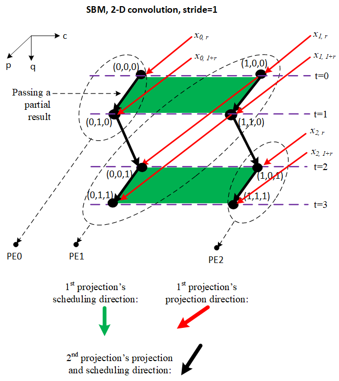
Figure 6. Applying 2 projections to 2-D convolution. In this design, we keep the outer loop r untouched, and transform only the inner loops (c, p, q). Every point is annotated with its corresponding indices (c, p, q). For simplicity, the broadcasting of weights is not drawn.

6. Experiments

We have prototyped our approach on top of Susy (Lai et al., 2020), generating CM code for Intel GPUs . In this section, we evaluated the performance of generated code that implements the above 1-D and 2-D convolution designs described in Section 3.1 and  5. The first SBM design is programmed using about 10 to 20 minutes, and with slight modification of the UREs and space-time transform of the SBM design, all the other designs are quickly expressed in a few minutes. This demonstrates the generality and flexibility of our approach, and the productivity of exploring the design space.

Our testing machine has an Intel HD Graphics 620 GPU, which is manufactured in 14 nm process based on Gen9.5 Kaby Lake architecture, runs at 1.1 GHZ and shares 3.9 GB memory with an Core i5 CPU. This GPU has 3 subslices; every subslice has 8 EUs, and every EU has 7 threads; every EU thread contains SIMD 8/16 lanes for 32/16-bit floats/integers, and 128 vector registers; each vector register has 32 bytes. EU threads in the same subslice can communicate through shared memory.

This GPU has hardware support for 1- and 2-D convolution of output size 16*1 and 16*4. Every subslice of the GPU has a sampler, which fetches data from external memory, and performs operations including convolution. The CM language has two interface functions, cm_va_1d_convolve and cm_va_2d_convolve, to allow programmers to use the hardware samplers to perform convolutions directly.

We issue over 10 millions of threads for sufficiently long and stable execution time, 56 threads as a group, each thread running a convolution (1-D or 2-D, performed by the sampler or our software systolic arrays, with filter size equal to 2 or 5 for 1-D convolution or 2x2 or 5x5 for 2-D convolution, with stride equal to 1 or 2), and every thread generating a 16*4 output matrix. Then we calculate the throughput by the number of output data divided by the execution time. We report the relative performance of our systolic arrays by their throughputs divided by the throughputs of the samplers for the same convolutions. We choose to compare with the sampler since it is a specialized hardware, and thus sets up a high-performance baseline.

6.1. Summary of the Experimental Results

Briefly, our experiments yield the following results:

1. All our systolic designs work correctly with reasonable performance. Among them, SBM and FBS show the best performance: they are 47%-59% faster than the samplers for 1-D convolution, and are close to or faster than the samplers for 2-D convolution with a small filter size. Profiling shows this is due to their efficient usage of the SIMD lanes in the EUs. Qualitative analysis also confirms that they are the best designs.

2. The sampler-performed convolutions are limited in flexibility since the filter size can not exceed 8, and the stride is fixed to 1. In comparison, our software systolic arrays are not limited to any specific filter size or stride.

Table 3. 1-D Convolution Experimental Results.

	SBM		BSM		FSM		BFS		FFS		FBS
Filter size	2	5	2	5	2	5	2	5	2	5	2	5
Relative performance	157%	147%	67%	49%	56%	39%	56%	48%	33%	30%	159%	157%

Table 4. Analytical Model for 1 1-D Convolution (filter size=5)

	SBM	BSM	FSM	BFS	FFS	FBS
Outturn a	3.2	0.8	0.8	0.8	0.46	3.2
Utilization b	80%	80%	80%	25%	14%	100%
Reg usage	80	25	35	80	112	80

^a Equals 16/(#time steps)

^b Equals 16* (filter size)/(#SIMD lanes * #time steps)

Table 5. 2-D Convolution Experimental Results

	SBM		FBS
Filter size	2x2	5x5	2x2	5x5
Relative performance	92%	20%	114%	24%

6.2. Detailed Results

Table 3 shows the performance of our designs for 1-D convolution. SBM and FBS with a 5x5 filter show outstanding performance among all the other designs. All the other designs show inferior performance.

The difference in performance among these designs is expected. We can derive an analytical model for the designs shown in Table 4. To be simple, consider 1 convolution with filter size of 5. Every design outputs 16 results. Thus the average outturn is 16/(#time steps). Furthermore, a design performs (#SIMD lanes * #time steps) number of operations in a convolution, but among them only 16 * (filter size) number of operations contribute to useful results, and thus the utilization rate of the SIMD lanes equals 16 * (filter size) / (#SIMD lanes * #time steps). Finally we can count the number of scalar registers the compiler allocates for each design (A vector register is counted as multiple scalar registers). A design with high outturn, high utilization of SIMD lanes, and preferably lower register usage, is a good design, and expected to yield high performance. As we can see from the analytical mode in Table 4, SBM and FBS excel at both outturn and utilization, while the other designs are inferior.

Table 5 reports the performance of 2-D convolution for filter size of 2x2 and 5x5 with stride of 1. They demonstrate multi-projection and generality of our approach. The SBM design has been shown in Fig. 6; the FBS design is similar, and simply converts a 2-D convolution into multiple FBS 1-D convolutions. We will work on the other designs of 2-D convolution in future.

As we can see, the two designs are close to or surpass the performance of the samplers for 2-D convolutions when the filter size is small, but the performance drops sharply as the filter size increases. As there is no public document on how the samplers implement 2-D convolution, we have difficulty in understanding the performance difference and will contact Intel experts for help.

7. Related Work

Systolic arrays are usually built on spatial architectures like FPGAs and CGRAs, or built as ASIC circuits (H.T. Kung, 1982; Saldaña-González and Arias-Estrada, 2009; Hrabovsky et al., 2017; Buyukkurt and Najjar, 2008; Settle, 2013; Jouppi et al., 2017).

The Alpha language (Verge et al., 1991) is a functional language to express and transform iterative algorithms, and generate systolic arrays. Programmers have limited control on optimizations.

T2S (Rong, 2017) is a methodology that addresses high-performance high productivity programming on spatial architectures like FPGAs. T2S advocates a programming style that separates concerns by separating a temporal definition from a spatial mapping. T2S-Tensor (Srivastava et al., 2019) is the first system that realizing the principle of T2S, built upon the Halide language and compiler framework (Ragan-Kelley et al., 2013). T2S-Tensor creates asynchronous (i.e. wavefront) arrays, and has demonstrated impressive productivity and performance for dense matrix multiply, MTTKRP, TTM and TTMc on an Arria-10 FPGA and a research CGRA. However, T2S-Tensor relies on loop unrolling, which permits creating only a limited set of systolic arrays.

Susy (Lai et al., 2020) introduces UREs and space-time transforms into T2S-Tensor, and generates synchronous arrays on FPGAs. It achieves performance for matrix multiply similar to that of T2S-Tensor, but with much less block RAM usage: thanks to space-time transform, the register requirement of a recurrent variable can be precisely calculated. The limitation of Susy is that it allows only a single projection along a loop dimension.

GPUs are usually programmed in SIMT style in CUDA or OpenCL. Our approach takes advantage of the fact that the underlying execution units actually work in SIMD fashion, and therefore, we enable a mixed style of SIMT + SIMD.

Our approach leverages Susy, breaks its limitations and extends it to GPUs, with substantial innovation as summarized in Section 1. We are not aware of any other language and compiler for creating systolic arrays on GPUs.

8. Conclusion and Future Work

We have presented a programming language and compiler, for the first time to the best of our knowledge, for quickly building high-performance systolic arrays on GPUs. Based on UREs and space-time transform, our approach has a solid mathematical foundation and should be able to cover a wide range of applications. Primitive experimental results on Intel GPUs have confirmed the generality and flexibility of this approach, and demonstrated its promise in performance and productivity.

In future, we will build a design space explorer that can automatically enumerate valid systolic designs for a workload, and search for the best candidates, and we will extend the system to CPUs as well, since CPUs also have SIMD execution units.

- (1)
- Alba and Vidal (2012) Enrique Alba and Pablo Vidal. 2012. Systolic Optimization on GPU Platforms. In Computer Aided Systems Theory – EUROCAST 2011, Roberto Moreno-Díaz, Franz Pichler, and Alexis Quesada-Arencibia (Eds.). Springer Berlin Heidelberg, Berlin, Heidelberg, 375–383.
- Buyukkurt and Najjar (2008) Betul Buyukkurt and Walid A. Najjar. 2008. Compiler Generated Systolic Arrays For Wavefront Algorithm Acceleration on FPGAs. In In International Conference on Field Programmable Logic and Applications.
- Chen et al. (2019) Peng Chen, Mohamed Wahib, Shinichiro Takizawa, Ryousei Takano, and Satoshi Matsuoka. 2019. A Versatile Software Systolic Execution Model for GPU Memory-Bound Kernels. In Proceedings of the International Conference for High Performance Computing, Networking, Storage and Analysis (SC ’19). Association for Computing Machinery, New York, NY, USA, Article 53, 81 pages. https://doi.org/10.1145/3295500.3356162
- Chen and Kung (1998) Yen-Kuang Chen and S.Y. Kung. 1998. A Systolic Design Methodology with Application to Full-Search Block-Matching Architectures. Journal of VLSI signal processing systems for signal, image and video technology 19 (1998), 51–77.
- Fatahalian and Houston (2008) Kayvon Fatahalian and Mike Houston. 2008. A Closer Look at GPUs. Commun. ACM 51, 10 (Oct. 2008), 50–57. https://doi.org/10.1145/1400181.1400197
- Hrabovsky et al. (2017) J. Hrabovsky, P. Segec, M. Moravcik, and J. Papan. 2017. Systolic-based 2D convolver for CNN in FPGA. In 2017 15th International Conference on Emerging eLearning Technologies and Applications (ICETA). 1–7. https://doi.org/10.1109/ICETA.2017.8102485
- H.T. Kung (1982) H.T. Kung. 1982. Why systolic architectures? Computer 15, 1 (1982), 37–46.
- Hughey (1991) Richard Paul Hughey. 1991. Programmable Systolic Arrays. Ph.D. Dissertation. Brown University, Providence, Rhode Island.
- Intel (2015) Intel. 2015. The Compute Architecture of Intel Processor Graphics Gen9. https://software.intel.com/sites/default/files/managed/c5/9a/The-Compute-Architecture-of-Intel-Processor-Graphics-Gen9-v1d0.pdf.
- Intel (2017) Intel. 2017. Accelerating Genomics Research with OpenCL™ and FPGAs. https://www.intel.com/content/dam/altera-www/global/en_US/pdfs/literature/wp/wp-accelerating-genomics-opencl-fpgas.pdf
- Intel (2019a) Intel. 2019a. Intel Design Examples. https://www.intel.com/content/www/us/en/ programmable/support/support-resources/design-examples/design-software/opencl/matrix-multiplication.html.
- Intel (2019b) Intel. 2019b. Intel(R) C for Metal Compiler. https://github.com/intel/cm-compiler.
- Jo et al. (2018) J. Jo, S. Kim, and I. Park. 2018. Energy-Efficient Convolution Architecture Based on Rescheduled Dataflow. IEEE Transactions on Circuits and Systems I: Regular Papers 65, 12 (Dec 2018), 4196–4207. https://doi.org/10.1109/TCSI.2018.2840092
- Jouppi et al. (2017) Norman P. Jouppi, Cliff Young, Nishant Patil, David Patterson, Gaurav Agrawal, Raminder Bajwa, Sarah Bates, Suresh Bhatia, Nan Boden, Al Borchers, Rick Boyle, Pierre-luc Cantin, Clifford Chao, Chris Clark, Jeremy Coriell, Mike Daley, Matt Dau, Jeffrey Dean, Ben Gelb, Tara Vazir Ghaemmaghami, Rajendra Gottipati, William Gulland, Robert Hagmann, C. Richard Ho, Doug Hogberg, John Hu, Robert Hundt, Dan Hurt, Julian Ibarz, Aaron Jaffey, Alek Jaworski, Alexander Kaplan, Harshit Khaitan, Daniel Killebrew, Andy Koch, Naveen Kumar, Steve Lacy, James Laudon, James Law, Diemthu Le, Chris Leary, Zhuyuan Liu, Kyle Lucke, Alan Lundin, Gordon MacKean, Adriana Maggiore, Maire Mahony, Kieran Miller, Rahul Nagarajan, Ravi Narayanaswami, Ray Ni, Kathy Nix, Thomas Norrie, Mark Omernick, Narayana Penukonda, Andy Phelps, Jonathan Ross, Matt Ross, Amir Salek, Emad Samadiani, Chris Severn, Gregory Sizikov, Matthew Snelham, Jed Souter, Dan Steinberg, Andy Swing, Mercedes Tan, Gregory Thorson, Bo Tian, Horia Toma, Erick Tuttle, Vijay Vasudevan, Richard Walter, Walter Wang, Eric Wilcox, and Doe Hyun Yoon. 2017. In-Datacenter Performance Analysis of a Tensor Processing Unit. In Proceedings of the 44th Annual International Symposium on Computer Architecture (ISCA ’17). Association for Computing Machinery, New York, NY, USA, 1–12. https://doi.org/10.1145/3079856.3080246
- Kung and Leiserson (1978) H.T. Kung and C.E. Leiserson. 1978. Systolic Arrays for (VLSI). Technical Report CMU-CS-79-103. Carnegie Mellon University, Pittsburgh, Pennsylvania.
- Kung et al. (1987) Sun-Yuan Kung, Sheng-Chun Lo, et al. 1987. Optimal systolic design for the transitive closure and the shortest path problems. IEEE Trans. Comput. 100, 5 (1987), 603–614.
- Kurzak et al. (2013) J. Kurzak, P. Luszczek, M. Gates, I. Yamazaki, and J. Dongarra. 2013. Virtual Systolic Array for QR Decomposition. In 2013 IEEE 27th International Symposium on Parallel and Distributed Processing. 251–260. https://doi.org/10.1109/IPDPS.2013.119
- Lai et al. (2020) Yi-Hsiang Lai, Hongbo Rong, Size Zheng, Weihao Zhang, Xiuping Cui, Yunshan Jia, Jie Wang, Brendan Sullivan, Zhiru Zhang, Yun Liang, Youhui Zhang, Jason Cong, Nithin George, Jose Alvarez, Christopher Hughes, and Pradeep Dubey. 2020. SuSy: A Programming Model for Productive Construction of High-Performance Systolic Arrays on FPGAs. To appear at ICCAD 2020.
- NVidia (2020) NVidia. 2020. CUDA C++ PROGRAMMING GUIDE. https://docs.nvidia.com/pdf/CUDA_C_Programming_Guide.pdf.
- Quinton (1984) Patrice Quinton. 1984. Automatic Synthesis of Systolic Arrays from Uniform Recurrent Equations. In Proceedings of the 11th Annual International Symposium on Computer Architecture (ISCA ’84). ACM, New York, NY, USA, 208–214. https://doi.org/10.1145/800015.808184
- Quinton (1987) Patrice Quinton. 1987. An introduction to systolic architectures. In Future Parallel Computers, P. Treleaven and M. Vanneschi (Eds.). Springer Berlin Heidelberg, Berlin, Heidelberg, 387–400.
- Ragan-Kelley et al. (2013) Jonathan Ragan-Kelley, Connelly Barnes, Andrew Adams, Sylvain Paris, Frédo Durand, and Saman Amarasinghe. 2013. Halide: A Language and Compiler for Optimizing Parallelism, Locality, and Recomputation in Image Processing Pipelines. In Proceedings of the 34th ACM SIGPLAN Conference on Programming Language Design and Implementation (PLDI ’13). ACM, New York, NY, USA, 519–530. https://doi.org/10.1145/2491956.2462176
- Rong (2017) Hongbo Rong. 2017. Programmatic Control of a Compiler for Generating High-performance Spatial Hardware. CoRR abs/1711.07606 (2017). arXiv:1711.07606 http://arxiv.org/abs/1711.07606
- Saldaña-González and Arias-Estrada (2009) Griselda Saldaña-González and Miguel Arias-Estrada. 2009. FPGA Based Acceleration for Image Processing Applications. In Image Processing, Yung-Sheng Chen (Ed.). IntechOpen. Available from: https://www.intechopen.com/books/image-processing/fpga-based-acceleration-for-image-processing-applications.
- Settle (2013) Sean O Settle. 2013. High-performance Dynamic Programming on FPGAs with OpenCL. In 2013 IEEE High Performance Extreme Computing Conference(HPEC ’13).
- Srivastava et al. (2019) Nitish Srivastava, Hongbo Rong, Prithayan Barua, Guanyu Feng, Huanqi Cao, Zhiru Zhang, David Albonesi, Vivek Sarkar, Wenguang Chen, Paul Petersen, Geoff Lowney, Adam Herr, Christopher Hughes, Timothy Mattson, and Pradeep Dubey. 2019. ”T2S-Tensor : Productively Generating High-Performance Spatial Hardware for Dense Tensor Computation”. In Proceedings of the International Symposium on Field-Programmable Custom Computing Machines (FCCM).
- Vanbroekhoven et al. (2007) Peter Vanbroekhoven, Gerda Janssens, Maurice Bruynooghe, and Francky Catthoor. 2007. A Practical Dynamic Single Assignment Transformation. ACM Trans. Des. Autom. Electron. Syst. 12, 4, Article 40 (Sept. 2007). https://doi.org/10.1145/1278349.1278353
- Verge et al. (1991) Hervé Verge, Christophe Mauras, and Patrice Quinton. 1991. The ALPHA Language and Its Use for the Design of Systolic Arrays. J. VLSI Signal Process. Syst. 3, 3 (Sept. 1991), 173–182. https://doi.org/10.1007/BF00925828
- Wang et al. (2017) J. Wang, X. Xie, and J. Cong. 2017. Communication Optimization on GPU: A Case Study of Sequence Alignment Algorithms. In 2017 IEEE International Parallel and Distributed Processing Symposium (IPDPS). 72–81.
- Wei et al. (2017) Xuechao Wei, Cody Hao Yu, Peng Zhang, Youxiang Chen, Yuxin Wang, Han Hu, Yun Liang, and Jason Cong. 2017. Automated systolic array architecture synthesis for high throughput CNN inference on FPGAs. In Proceedings of the 54th Annual Design Automation Conference 2017. ACM, 29.
- Xue (1992) J. Xue. 1992. The Formal Synthesis of Control Signals for Systolic Arrays. Ph.D. Dissertation. Department of Computer Science, University of Edinburgh.
- Zehendner (2007) Eberhard Zehendner. 2007. Algorithms of Informatics. Chapter 16. Systolic Systems. Available: https://www.tankonyvtar.hu/en/tartalom/tamop425/0046_algorithms_of_informatics_volume2/ch04.html.