Luminous Type II Short-Plateau Supernovae 2006Y, 2006ai, and 2016egz: A Transitional Class from Stripped Massive Red Supergiants

Abstract

The diversity of Type II supernovae (SNe II) is thought to be driven mainly by differences in their progenitor’s hydrogen-rich (H-rich) envelope mass, with SNe IIP having long plateaus ($\sim 100$ days) and the most massive H-rich envelopes. However, it is an ongoing mystery why SNe II with short plateaus (tens of days) are rarely seen. Here, we present optical/near-infrared photometric and spectroscopic observations of luminous Type II short-plateau SNe 2006Y, 2006ai, and 2016egz. Their plateaus of about $50$–$70$ days and luminous optical peaks ($\lesssim-18.4$ mag) indicate significant pre-explosion mass loss resulting in partially stripped H-rich envelopes and early circumstellar material (CSM) interaction. We compute a large grid of MESA+STELLA single-star progenitor and light-curve models with various progenitor zero-age main-sequence (ZAMS) masses, mass-loss efficiencies, explosion energies, ⁵⁶Ni masses, and CSM densities. Our model grid shows a continuous population of SNe IIP–IIL–IIb-like light-curve morphology in descending order of H-rich envelope mass. With large ⁵⁶Ni masses ($\gtrsim 0.05\,M_{\odot}$), short-plateau SNe II lie in a confined parameter space as a transitional class between SNe IIL and IIb. For SNe 2006Y, 2006ai, and 2016egz, our findings suggest high-mass red supergiant (RSG) progenitors ($M_{\rm ZAMS}\simeq 18$–$22\,M_{\odot}$) with small H-rich envelope masses ($M_{\rm H_{\rm env}}\simeq 1.7\,M_{\odot}$) that have experienced enhanced mass loss ($\dot{M}\simeq 10^{-2}\,M_{\odot}\,{\rm yr}^{-1}$) for the last few decades before the explosion. If high-mass RSGs result in rare short-plateau SNe II, then these events might ease some of the apparent underrepresentation of higher-luminosity RSGs in observed SN II progenitor samples.

2021 May 25

1 Introduction

The majority of massive stars (zero-age main-sequence masses $M_{\mathrm{ZAMS}}\gtrsim 8\,M_{\odot}$) end their lives when their iron cores collapse and explode as hydrogen-rich (H-rich), Type II supernovae (SNe II) (Smartt, 2009, 2015). The difference in progenitor’s H-rich envelope mass at the moment of core collapse likely results in different SN II subtypes (e.g., Nomoto et al. 1995; Heger et al. 2003; Dessart et al. 2011, 2016b; Eldridge et al. 2017, 2018): SNe IIP (light-curve plateau of $\sim 100$ days); SNe IIL (linear decline light curve); and SNe IIb (spectrum dominated initially by hydrogen and then by helium), in descending order (see Arcavi 2017 for a review). SNe IIn show narrow H emission lines, indicating strong circumstellar material (CSM) interaction (see Smith 2017 for a review). Based on the direct progenitor identifications in pre-explosion images, the current consensus is that the progenitors are red supergiants (RSGs) for SNe IIP; yellow supergiants in a binary system for SNe IIb; luminous blue variables and RSGs/super-asymptotic giant branch stars for SNe IIn; and RSGs and/or yellow supergiants for SNe IIL, in descending order of confidence (see Van Dyk 2016 for a review).

The division between SNe IIP and IIL is both arbitrary and controversial because it is solely based on the shape of their photospheric-phase optical light curves (Barbon et al., 1979), while SNe IIb and IIn are spectroscopically distinct. There have been claims of distinct light-curve populations of SNe IIP and IIL (e.g., Arcavi et al. 2012; Faran et al. 2014), but larger light-curve samples have increased the support for a more continuous population (e.g., Anderson et al. 2014; Sanders et al. 2015; Galbany et al. 2016b; Valenti et al. 2016). While SNe IIP and IIL show a continuous range of spectroscopic properties in optical (e.g., Gutiérrez et al. 2017a, b), Davis et al. (2019) recently find a strong dichotomy of near-infrared (NIR) spectroscopic properties between SNe IIP and IIL, which may point to differences in the immediate environment.

In terms of the photospheric plateau duration, it is puzzling that SNe II with short plateaus (tens of days) are rarely observed (see e.g., Nakaoka et al. 2019 and Bostroem et al. 2020 for peculiar SNe IIb and IIL), despite analytical and numerical predictions that the plateau duration scales continuously with progenitor and explosion properties (Popov, 1993; Kasen & Woosley, 2009; Sukhbold et al., 2016; Goldberg et al., 2019). In a broader context of SN II population, it is also an outstanding question whether SNe IIP/L and IIb form a continuum or not (e.g., Arcavi et al. 2012; Faran et al. 2014; Pessi et al. 2019).

The increasing sample size of SNe IIP/L suggests that CSM interaction, resulting from violent pre-explosion mass loss, plays a key role even when their spectra do not show IIn-like Balmer emission lines. By fitting numerical models to the Valenti et al. (2015, 2016) light-curve sample, Morozova et al. (2017, 2018) show that SNe IIP from RSG progenitors with CSM interaction can reproduce SNe IIL. They also show that CSM interaction is required in even normal SNe IIP to reproduce the rapid UV-optical rise in the models (see also Moriya et al. 2011, 2017, 2018; Förster et al. 2018).

The observed RSG population (in the Milky Way, Magellanic Clouds, M31, and M33) lies in a luminosity range of $4.5\lesssim{\rm log}_{10}(L/L_{\odot})\lesssim 5.5$, implying their ZAMS mass range of $\sim 9$–$25\,M_{\odot}$ based on theoretical stellar tracks (e.g., Levesque et al. 2005, 2006; Massey et al. 2009; Drout et al. 2012; Gordon et al. 2016). However, Smartt (2009, 2015) show that the best-fit cumulative Salpeter initial mass function (IMF; Salpeter 1955) on 26 pre-explosion detections/limits of SNe IIP/L progenitors truncates below the high-luminosity end of RSGs, translating to a ZAMS mass upper limit of $\lesssim 18\,M_{\odot}$. This is referred to as the red supergiant problem, since there seems to be a lack of SNe II with identified progenitors in the range $\sim 18$–$25\,M_{\odot}$. Due to the complicated evolution of terminal massive stars and observational uncertainties in dust extinction and bolometric correction, the statistical significance and robustness of the RSG problem has been a highly debated topic (e.g., Walmswell & Eldridge 2012; Eldridge et al. 2013; Kochanek 2014; Meynet et al. 2015; Sukhbold et al. 2016; Adams et al. 2017; Davies & Beasor 2018).

Here, we report optical/NIR photometry and spectroscopy of Type II SNe 2006Y, 2006ai, and 2016egz. In Sections 2 and 3, we summarize their discoveries, follow-up observations, and data reduction. In Section 4, we analyze their host galaxies, light curves, and spectra, in addition to producing a large single-star model grid by varying different progenitor and explosion properties. This reveals their transitional nature between SNe IIL and IIb with small H-rich envelope mass, high progenitor ZAMS mass, and dense CSM estimates. As such, we discuss their formation channel and implications for the RSG problem in Section 5. Finally, we summarize our findings and draw conclusions in Section 6.

2 Discoveries

Luckas et al. (2006b) discovered SN 2006Y on 2006 February 3.58 (UT dates are used throughout) at 17.7 mag at $\text{R.A.}=07^{\text{h}}13^{\text{m}}17^{\text{s}}.17$ and $\text{Dec.}=-51^{\circ}41^{\prime}18".8$ with a subsequent detection on 2006 February 7.60 at 17.3 mag and last non-detection limit on 2006 January 27.59 at 18.5 mag, using the unfiltered $35$ cm Tenagra telescope at Perth, Australia. With the same instrumental setup, Luckas et al. (2006a) discovered SN 2006ai on 2006 February 17.54 at 16.2 mag at $\text{R.A.}=07^{\text{h}}29^{\text{m}}52^{\text{s}}.16$ and $\text{Dec.}=-84^{\circ}02^{\prime}20".5$ with a subsequent detection on 2006 February 19.52 at 16.0 mag and last non-detection limit on 2005 December 16.79 at 18.5 mag. Morrell & Folatelli (2006) obtained optical spectra of SNe 2006Y and 2006ai on February 27.14 and March 5.12, respectively, with the Las Campanas $2.5$ m du Pont telescope through the Carnegie Supernova Project-I (CSP-I; Hamuy et al. 2006), classifying them as SNe II. CSP-I also obtained optical spectra of the host galaxies of SNe 2006Y and 2006ai and measured redshifts of $z=0.0336\pm 0.0001$ and $0.0158\pm 0.0001$, respectively.

The All-Sky Automated Survey for Supernovae (ASAS-SN; Shappee et al. 2014) discovered SN 2016egz (ASASSN-16hn) on 2016 July 24.32 at 16.1 mag at $\text{R.A.}=00^{\text{h}}04^{\text{m}}03^{\text{s}}.854$ and $\text{Dec.}=-34^{\circ}48^{\prime}51".87$ with a last non-detection limit on 2016 July 17.23 at 17.4 mag, using the V-band $14$ cm ASAS-SN Cassius telescope at Cerro Tololo, Chile (Brown, 2016). A prediscovery detection on 2016 July 21.26 at 15.5 mag with the same instrumental setup was retrieved via the ASAS-SN light-curve server (Shappee et al., 2014; Kochanek et al., 2017). Fraser et al. (2016) obtained an optical spectrum of SN 2016egz on 2016 July 26.25 with the European Southern Observatory (ESO) $3.58$ m New Technology Telescope (NTT) through the Public ESO Spectroscopic Survey for Transient Objects (PESSTO; Smartt et al. 2015), classifying it as a young SN II at $z=0.0232\pm 0.0003$ of the host galaxy, GALEXASC J000403.88-344851.6 (Colless et al., 2003).

Given the tight last non-detection limits, we estimate the explosion epochs of SNe 2006Y and 2016egz by simply taking the midpoint of the last non-detection and the first detection with the error being the estimated explosion epoch minus the last non-detection. This yields $\text{MJD}_{0}=53766.1\pm 3.4$ and $57588.2\pm 2.0$ for SNe 2006Y and 2016egz, respectively. As there is no constraining last non-detection limit for SN 2006ai, we adopt the explosion epoch estimate $\text{MJD}_{0}=53781.6\pm 5.0$ ($\sim 1.9$ days before the discovery) from the spectral matching technique of Anderson et al. (2014) and Gutiérrez et al. (2017a). This is reasonable given the early rising light curves (see $\S$3). For each SN, we use the explosion epoch as a reference epoch for all phases. We assume a standard Lambda cold dark matter cosmology with $H_{0}=71.0$  km s^-1 Mpc^-1, $\Omega_{\Lambda}=0.7$, and $\Omega_{m}=0.3$, and convert the redshifts to luminosity distances: $d_{L}=146$ Mpc ($\mu=35.8$ mag), $67.5$ Mpc ($34.1$ mag), and $100$ Mpc ($35.0$ mag), respectively, for SNe 2006Y, 2006ai, and 2016egz.

3 Observations and Data Reduction

Figure 1: Host-subtracted and extinction-corrected light curves of SNe 2006Y, 2006ai, and 2016egz. Error bars denote $1\sigma$ uncertainties and are sometimes smaller than the marker size. Note the similar luminous V-band peaks ($\lesssim-18.2$ mag) and short V-band plateaus ($\sim 50$–$70$ days). The tail of SN 2006Y is not well sampled, while those of SNe 2006ai and 2016egz are roughly consistent with ⁵⁶Co decay.

Figure 2: Extinction-corrected spectral series of SNe 2006Y, 2006ai, and 2016egz. Approximate evolutionary phases are given as: shock for shock-cooling phase with a mostly blue featureless continuum; photo for optically thick photospheric phase with prominent hydrogen P Cygni features; and nebular for optically thin nebular phase with forbidden emission lines (e.g., [O i] $\lambda\lambda 6300,6364$). Note that the narrow emission lines (e.g., H$\alpha$ and H$\beta$) and the late-time ($\gtrsim 70$ d) blue continuum with the $4000\,\textup{\AA}$ break are host contaminants, as seen in the host (i.e., the last) spectra.

For SNe 2006Y and 2006ai, uBgVri optical and YJH NIR photometry were obtained through CSP-I. Standard reduction techniques were applied to all images (e.g., Stritzinger et al. 2011). Then deep template observations obtained once the SN had sufficiently faded from detection were used to subtract the underlying host galaxy emission. Photometry of the SN was computed differentially with respect to a local sequence of stars, together with definitive photometry in the standard ugri (Smith et al., 2002), BV (Landolt, 1992), and YJH (Persson et al., 1998) photometric systems, and calibrated to standard star fields observed on photometric nights (see Krisciunas et al. 2017 for a detailed description of the above). The V-band light curves presented here are an updated version to those included in the Anderson et al. (2014) sample. CSP-I spectroscopy of SNe 2006Y and 2006ai has already been published in Gutiérrez et al. (2017a), and the reader is referred to that publication for more details.

For SN 2016egz, Las Cumbres Observatory BgVri-band data were obtained with the SBIG and Sinistro cameras on the network of 1-m telescopes at Sutherland (South Africa), the Cerro Tololo Inter-American Observatory (Chile), and Siding Spring (Australia) (Brown et al., 2013), through the Supernova Key Project and Global Supernova Project. Using lcogtsnpipe (Valenti et al., 2016), a PyRAF-based photometric reduction pipeline, point-spread function fitting was performed. Reference images were obtained with a Sinistro camera after the SN faded, and image subtraction was performed using PyZOGY (Guevel & Hosseinzadeh, 2017), an implementation in Python of the subtraction algorithm described in Zackay et al. (2016). BV- and gri-band data were calibrated to Vega (Stetson, 2000) and AB (Albareti et al., 2017) magnitudes, respectively, using standard fields observed on the same night by the same telescope as the SN.

Las Cumbres Observatory optical spectra for SN 2016egz were taken with the FLOYDS spectrographs mounted on the 2m Faulkes Telescope North (FTN) and South (FTS) at Haleakala (USA) and Siding Spring (Australia), respectively, through the Supernova Key Project and Global Supernova Project. A $2\arcsec$ slit was placed on the target along the parallactic angle (Filippenko, 1982). One-dimensional spectra were extracted, reduced, and calibrated following standard procedures using floyds_pipeline (Valenti et al., 2014). Additional optical spectra of the SN and host galaxy were obtained by PESSTO and extended PESSTO (ePESSTO) with NTT ($+$EFOSC2). EFOSC2 spectra were reduced and calibrated in a standard manner using a custom built pipeline for the PESSTO project (Smartt et al., 2015).

All photometry and spectroscopy of SNe 2006Y, 2006ai, and 2016egz are presented in Figures 1 and 2, respectively, and will be available for download via the Open Supernova Catalog (Guillochon et al., 2017) and the Weizmann Interactive Supernova Data Repository (WISeREP; Yaron & Gal-Yam 2012). For SNe 2006Y, 2006ai, and 2016egz, no Na i D absorption is seen at the host redshift (Figure 2), indicating low host extinction at the SN position. Thus, we correct all photometry and spectroscopy only for the Milky Way extinction (Schlafly & Finkbeiner, 2011) of $A_{V}=0.347$, $0.337$, and $0.042$ mag for SNe 2006Y, 2006ai, and 2016egz, respectively, assuming the Fitzpatrick (1999) reddening law with $R_{V}=3.1$.

4 Analysis

4.1 Host Galaxies

Table 1: Host Galaxy Line Fluxes ($10^{-15}$ erg s^-1 cm^-2)

SN	[O ii] $\lambda 3727$	H$\beta$	[O iii] $\lambda 4959$	[O iii] $\lambda 5007$	H$\alpha$	[N ii] $\lambda 6583$	[S ii] $\lambda 6717$	[S ii] $\lambda 6731$
2006Y	$13.9\pm 0.3$	$2.89\pm 0.04$	$3.08\pm 0.07$	$9.87\pm 0.02$	$10.37\pm 0.04$	$0.86\pm 0.01$	$1.52\pm 0.04$	$1.06\pm 0.03$
2006ai	–	$37\pm 2$	$7.2\pm 0.3$	$18.4\pm 0.6$	$181\pm 3$	$54\pm 1$	$7.8\pm 0.6$	$45\pm 3$
2016egz	$5.08\pm 0.04$	$1.03\pm 0.04$	$1.95\pm 0.04$	$4.87\pm 0.02$	$4.62\pm 0.03$	$0.14\pm 0.01$	$0.13\pm 0.02$	$1.13\pm 0.02$

Table 2: Host Galaxy Properties

SN	$M_{B}$	Galaxy Class	${\rm SFR}(L_{\rm H\alpha})$	${\rm SFR}(L_{\rm[O~{}{\sc II}]})$	${\rm SFR}(L_{\rm GALEX})$	$12+{\rm log}_{10}({\rm O/H})$	$Z$
	(mag)		($M_{\odot}\,{\rm yr}^{-1}$)	($M_{\odot}\,{\rm yr}^{-1}$)	($M_{\odot}\,{\rm yr}^{-1}$)		($Z_{\odot}$)
2006Y	$-16.32$	Star forming	$0.2$	$0.5$	–	$8.32$ ($7.72$–$8.72$)	$0.35$
2006ai	$-19.22$	Star forming	$0.8$	–	–	$8.71$ ($8.50$–$8.91$)	$0.87$
2016egz	$-16.36$	Star forming	$0.04$	$0.08$	$0.15$	$8.20$ ($7.81$–$8.69$)	$0.27$

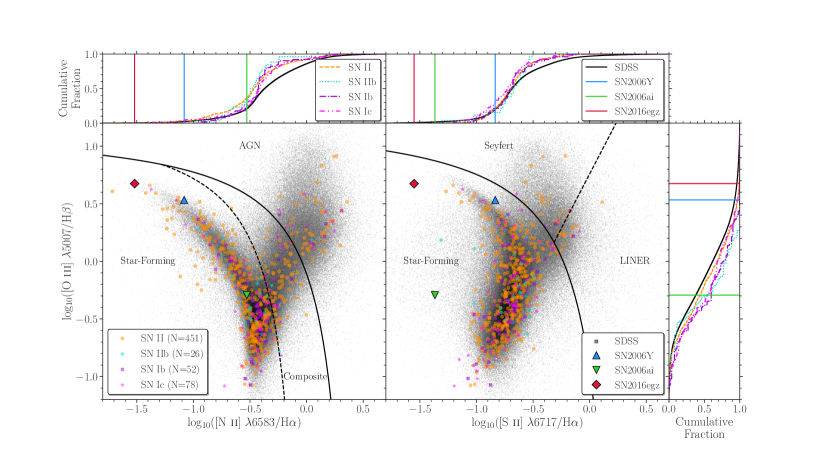
Figure 3: Comparison of the host galaxy BPT diagrams and cumulative fractions with respect to each axis of SNe 2006Y, 2006ai, and 2016egz with the SN sample of Graham (2019) and the Eighth Data Release of the Sloan Digital Sky Survey (SDSS DR8; Eisenstein et al. 2011; Aihara et al. 2011). The galaxy classification scheme is adopted from Kewley et al. (2006). Note that the host galaxies of SNe 2006Y, 2006ai, and 2016egz lie in the star-forming region with relatively low [N ii]/H$\alpha$ ($\lesssim 21\%$ and $\lesssim 37\%$ of SDSS and SN II host galaxies, respectively), [S ii]/H$\alpha$ ($\lesssim 21\%$ of SDSS and SN II host galaxies), and moderate-to-high [O iii]/H$\beta$ ($\lesssim 62\%$ and $\lesssim 56\%$ of SDSS and SN II host galaxies, respectively).

We measure host galaxy line fluxes by fitting a Gaussian profile to each line. The measurements are summarized in Table 1. In Figure 3, we place the host galaxies in Baldwin-Phillips-Terlevich (BPT) diagrams (Baldwin et al., 1981) based on the line ratios of [O iii] $\lambda 5007$/H$\beta$, [N ii] $\lambda 6583$/H$\alpha$, and [S ii] $\lambda 6717$/H$\alpha$. According to the Kewley et al. (2006) classification scheme, the host galaxies of SNe 2006Y, 2006ai, and 2016egz lie in the star-forming region in the BPT diagrams. Thus, we estimate star-formation rates (SFRs) from the H$\alpha$ and [O ii] $\lambda 3727$ fluxes using the calibrations summarized in Kennicutt (1998) and from the Galaxy Evolution Explorer (GALEX) photometry (Seibert et al. 2012, retrieved via NED) using the Salim et al. (2007) calibration where the measurements are available. These SFR estimates yield a range of $0.04$–$0.8\,M_{\odot}\,{\rm yr}^{-1}$. We also estimate host galaxy metallicities from the measured line ratios and various estimates using PyMCZ (Bianco et al., 2016). The weighted averages of $12+{\rm log}_{10}(\rm O/H)=8.20$–$8.71$ roughly correspond to $0.3$–$0.9\,Z_{\odot}$ (Asplund et al., 2009). The measured host galaxy properties are summarized in Table 2.

The host galaxies of SNe 2006Y, 2006ai, and 2016egz are star-forming galaxies at subsolar metallicities. They show relatively low [N ii]/H$\alpha$, [S ii]/H$\alpha$, and moderate-to-high [O iii]/H$\beta$ in the BPT comparisons with the SDSS and core-collapse supernova (CCSN) host galaxies (Figure 3). Compared to CCSN host galaxy samples, the host SFRs are relatively low ($\lesssim 25\%$ of CCSNe; Galbany et al. 2014), while the host metallicities span a wide range ($\sim 90\%$–$100\%$ of CCSNe; Anderson et al. 2016; Galbany et al. 2016a). SNe 2006Y, 2006ai, and 2016egz are also included in the Gutiérrez et al. (2018) SN II sample in low-luminosity host galaxies, in which they find that low-luminosity galaxies generally host SNe II with slower declining light curves and weaker absorption lines, but did not find strong correlations with plateau lengths or expansion velocities. Thus, short-plateau SNe, like 2006Y, 2006ai, and 2016egz, do not seem to have strong environmental preferences, although this merits future investigations with bigger samples given the rarity of these short-plateau SNe.

4.2 V-band and Bolometric Light Curves

Figure 4: Comparison of the unnormalized (top) and normalized to peak (bottom) light curves of SNe 2006Y, 2006ai, and 2016egz with SN II samples (gray transparent lines), including the archetypal SN IIP 1999em, the low-luminosity SNe IIP 2005cs and 2008bk, and the early-flash SN 2013fs. Error bars denote $1\sigma$ uncertainties and are sometimes smaller than the marker size. Note the similar high luminosity and short plateaus of SNe 2006Y, 2006ai, and 2016egz, which could be more pronounced, as their peaks are lower limits (i.e., not observed).

We fit a blackbody spectral energy distribution (SED) to every epoch of photometry containing at least three filters (excluding the r band owing to strong H$\alpha$ contamination) obtained within $0.3$ days of each other to estimate blackbody temperature and radius. Then we integrate the fitted blackbody SED over the full (and UBVRI: $3250$–$8900\textup{\AA}$) wavelength range to obtain bolometric (and pseudobolometric) luminosity at each epoch. Comparing the luminosity on the ⁵⁶Co tail to that of SN 1987A (Hamuy, 2003), we estimate ⁵⁶Ni masses of $0.062\pm 0.002\,M_{\odot}$ and $0.090\pm 0.005\,M_{\odot}$ for SNe 2006ai and 2016egz, respectively. Although the tail of SN 2006Y is not well sampled, we put a rough ⁵⁶Ni mass constraint of $0.06$–$0.09\,M_{\odot}$ based on the last V-band point and r- and i-band tail luminosity in between those of SNe 2006ai and 2016egz (Figure 1). These ⁵⁶Ni mass estimates are among the highest in the Anderson et al. (2014) and Valenti et al. (2016) samples.

The comparisons of the V-band and pseudobolometric light curves of SNe 2006Y, 2006ai, and 2016egz, respectively, with the Anderson et al. (2014) and Valenti et al. (2016) samples are shown in Figure 4. Anderson et al. (2014) include SNe 2006Y and 2006ai in their sample analysis and identify SN 2006Y as an outlier to many observed trends; it shows the fastest decline from the bright maximum followed by the shortest plateau length. The V-band light curves of SNe 2006ai and 2016egz show peak and plateau characteristics similar to SN 2006Y. The similarities stand out even more when their light curves are normalized to peak, showing one of the largest peak-to-tail luminosity contrasts and the shortest (optically thick) photospheric durations (Figure 4(a)). The peculiarities of SNe 2006Y and 2016egz could be even more extreme (compared to normal SN II population), given that their light-curve peaks are lower limits (not observed).

The similar characteristics can also be seen in the pseudobolometric light-curve comparison in Figure 4(b). In addition, the peaks and the following decline rates of SNe 2006Y, 2006ai, and 2016egz are brighter and steeper, respectively, than those of SN 2013fs (Yaron et al., 2017) whose early time ($\lesssim 5$ d) spectra show flash features (high-ionization CSM emission lines excited by the SN shock-breakout radiation; Gal-Yam et al. 2014; Khazov et al. 2016; Bruch et al. 2021). Various flash spectral and light-curve modeling have inferred high mass-loss rates for SN 2013fs, ranging from $\sim 0.001$–$0.1\,M_{\odot}\,{\rm yr}^{-1}$ for the last few years to decades before the explosion (e.g., Moriya et al. 2017; Morozova et al. 2017; Yaron et al. 2017, but see also Dessart et al. 2017; Soker 2021 and Kochanek 2019 for the possible alternatives from an extended envelope and binary interaction, respectively). Thus, the brighter and steeper peaks of SNe 2006Y, 2006ai, and 2016egz likely indicate the presence of similar or even denser CSM. However, we still do not see flash features, probably because the SN ejecta had already overrun the CSM by the time of our first spectra (Figure 2).

As first-order estimates for progenitor and explosion properties, we use the SN IIP light-curve scaling relations of Goldberg et al. (2019) that give degenerate parameter space for progenitor radius, ejecta mass ($M_{\rm ej}$), and explosion energy ($E_{\rm exp}$) based on the observed luminosity at day 50, plateau duration, and ⁵⁶Ni mass. We caution that these relations are not calibrated to short-plateau SNe, such as SNe 2006Y, 2006ai, and 2016egz, whose light curves start to drop from the plateaus around day 50, but nonetheless they should provide some crude estimates. The extra heating from ⁵⁶Ni extends plateau duration, but it is not the lack of ⁵⁶Ni that causes the short plateaus of SNe 2006Y, 2006ai, and 2016egz, given their high ⁵⁶Ni mass estimates. If we assume a typical RSG radius of $800\,R_{\odot}$, then H-rich $M_{\rm ej}\sim 1$, $2$, and $4\,M_{\odot}$ and $E_{\rm exp}\sim 0.3,0.4,0.8\times 10^{51}$ erg can be inferred, respectively, for SNe 2006Y, 2006ai, and 2016egz from the light-curve scaling relations. This suggests significant progenitor H-rich envelope stripping.

4.3 MESA+STELLA Progenitor and Light-curve Modeling

Figure 5: MESA+STELLA pseudobolometric light-curve models with a single ⁵⁶Ni mass ($M_{\rm Ni}=0.07\,M_{\odot}$), color coded by the H-rich envelope mass ($M_{\rm H_{\rm env}}$) at the core collapse. Arbitrary cuts in $M_{\rm H_{\rm env}}$ are applied to display each SN II subtype in each panel. Light curves with the same color in each panel come from the same progenitor model exploded with different energies ($E_{\rm exp}$); higher $E_{\rm exp}$ result in brighter, steeper, and shorter photospheric-phase light curves. Note the continuous population of SNe IIP–IIL–short-plateau–IIb in descending order of $M_{\rm H_{\rm env}}$ and the narrow $M_{\rm H_{\rm env}}$ window that results in short-plateau SNe.

Figure 6: MESA+STELLA pseudobolometric light-curve models with a single explosion energy ($E_{\rm exp}=10^{51}$ erg) from a representative progenitor model of each SN II subtype, color coded by the ⁵⁶Ni mass ($M_{\rm Ni}$). The initial shock-cooling phase is $M_{\rm Ni}$ independent, while the following photospheric phase is $M_{\rm Ni}$ dependent. Note that in the short-plateau $M_{\rm H_{\rm env}}$ range, the light curves also span IIL morphology with a lower $M_{\rm Ni}$ ($\lesssim 0.05\,M_{\odot}$).

Figure 7: Model-grid log likelihood distributions of the explosion energy ($E_{\rm exp}$) and the progenitor properties at the core collapse: H-rich envelope mass ($M_{\rm H_{\rm env}}$), total mass ($M_{\rm tot}$), and photospheric radius ($R_{\rm ph}$), along with the 20 best-fit light-curve models and the maximum likelihood parameters. In the 2D correlation plots, the brighter yellow regions correspond to the higher correlations, while the blank space corresponds to the parameter space that is not covered by the model grid. The $M_{\rm Ni}=0.07\,M_{\odot}$ grid is used to fit SNe 2006Y and 2006ai, while the $M_{\rm Ni}=0.1\,M_{\odot}$ grid is used to fit SN 2016egz. The overall light-curve morphology is reasonably well reproduced, except the early ($\lesssim 10$ days) excess emission, which we attribute to CSM interaction (Figures 8 and 9). Note the inferred small $M_{\rm H_{\rm env}}$ and high He-core masses ($M_{\rm He_{\rm core}}=M_{\rm tot}-M_{\rm H_{\rm env}}$) of $5.4$–$6.9\,M_{\odot}$ for SNe 2006Y, 2006ai, and 2016egz.

In order to explore the effect of H-rich envelope stripping in SN II light curves in more detail and to better extract physical parameters from the short-plateau light curves, we construct a large MESA (Paxton et al., 2011, 2013, 2015, 2018, 2019) + STELLA (Blinnikov et al., 1998, 2000, 2006; Blinnikov & Sorokina, 2004; Baklanov et al., 2005) single-star progenitor and light-curve model grid. For the MESA progenitor model grid, we vary ZAMS masses ($M_{\rm ZAMS}=10.0$–$25.0\,M_{\odot}$ with $2.5\,M_{\odot}$ increments) and wind scaling factors ($\eta_{\rm wind}=0.0$–$3.0$ with $0.1$ increments), while fixing subsolar ZAMS metallicity ($Z=0.3\,Z_{\odot}$) and no rotation ($\nu/\nu_{\rm crit}=0$). For the MESA explosion model grid, we vary explosion energies ($E_{\rm exp}=0.4$–$2.0\times 10^{51}$ erg with $0.2\times 10^{51}$ erg increments) and ⁵⁶Ni masses ($M_{\rm Ni}=0.04$, $0.07$, and $0.1\,M_{\odot}$) for each progenitor model. Then we hand off these explosion models to STELLA to produce synthetic light curves and expansion velocities. A more detailed description of the model grid is presented in Appendix A.

The full light-curve model grid with $M_{\rm Ni}=0.07\,M_{\odot}$ (totaling 1,303 models) is shown in Figure 5. This shows SN II subtypes as part of a continuous population, delineated by their H-rich envelope mass ($M_{\rm H_{\rm env}}$; we use the 20% mass fraction point $X({\rm H})\geq 0.2$). Short-plateau SNe represent a transitional class between SNe IIL and IIb in a narrow $M_{\rm H_{\rm env}}$ window ($\Delta M_{\rm H_{\rm env}}\sim 1.2\,M_{\odot}$). This is likely why these short-plateau SNe are so rare. The SN II plateau slope correlations with the maximum brightness and plateau duration (e.g., Anderson et al. 2014; Sanders et al. 2015; Galbany et al. 2016b; Valenti et al. 2016) are also naturally reproduced with some scatter by varying $M_{\rm H_{\rm env}}$ and $E_{\rm exp}$. As the population is rather continuous, the applied $M_{\rm H_{\rm env}}$ cuts are somewhat arbitrary and mainly for presentation purposes.

In order to demonstrate the effect of ⁵⁶Ni heating on the SN II light curves, we use a finer $M_{\rm Ni}$ grid spacing ($0.00$–$0.10\,M_{\odot}$ with $0.01\,M_{\odot}$ increments) for a representative model of each SN II subtype and show their light curves in Figure 6. The early phase is $M_{\rm Ni}$ independent, as it is powered by shock cooling. For the SN IIP/L models, the extra heating from ⁵⁶Ni extends the photospheric-phase duration (Kasen & Woosley, 2009; Goldberg et al., 2019; Kozyreva et al., 2019), but does not affect the overall IIP/L light-curve morphology. For the short-plateau SN models, on the other hand, the plateau phase is dominantly powered by ⁵⁶Ni heating (unlike those of the SN IIP models, but rather similar to the second peak of the SN IIb models), and the light curves result in IIL morphology with lower $M_{\rm Ni}$ ($\lesssim 0.05\,M_{\odot}$). This suggests the high $M_{\rm Ni}$ preference of short-plateau SNe.

Using the Binary Population and Spectral Synthesis Version 2 (BPASS v2; Eldridge et al. 2017) and the SuperNova Explosion Code (SNEC; Morozova et al. 2015) with a single $E_{\rm exp}=10^{51}$ erg and $M_{\rm Ni}=0.05\,M_{\odot}$, Eldridge et al. (2018) show a similar SN II population trend with respect to the total progenitor hydrogen mass ($M_{\rm H}$) and note the small population of short-plateau SNe ($\sim 4.7\%$ of all SNe II). They find a lower $M_{\rm H}$ range for SNe IIL ($0.003$–$0.7\,M_{\odot}$) than short-plateau ($0.3$–$2.0\,M_{\odot}$), compared to our model grid of SNe IIL ($1.3$–$3.1\,M_{\odot}$) and short-plateau ($0.45$–$1.3\,M_{\odot}$). But we do not consider this as a serious conflict as the subtype classifications are again ambiguous and also sensitive to other physical parameters (e.g., $E_{\rm exp}$ and $M_{\rm Ni}$ as shown in Figures. 5 and 6). A more detailed analyses of our MESA+STELLA model grid and its comparisons to observed SN II samples will be presented in a future publication (Hiramatsu et al., in prep.). In this work, we focus on its application to short-plateau SNe.

The short-plateau SN models come from massive progenitors ($M_{\rm ZAMS}\geq 17.5\,M_{\odot}$) with strong wind mass loss ($\eta_{\rm wind}\geq 1.2$) stripping significant amounts of the H-rich envelope ($\gtrsim 9\,M_{\odot}$). We caution that this could partially be due to a modeling bias as the wind mass loss is more sensitive to the choice of $\eta_{\rm wind}$ for more massive progenitors. But we also note that $15.0\,M_{\odot}$ progenitors within the short-plateau $M_{\rm H_{\rm env}}$ range (modeled with $\eta_{\rm wind}=3.4$; not included in the grid) do not result in short-plateau SNe, but IIL, even with $M_{\rm Ni}=0.1\,M_{\odot}$. With binary interactions, Eldridge et al. (2018) find a wider $M_{\rm ZAMS}$ range ($7$–$25\,M_{\odot}$) for short-plateau SNe. Thus, it is useful to have independent means of estimating $M_{\rm ZAMS}$ for cross checking (e.g., direct progenitor identification and nebular spectra; see $\S$4.6 for nebular spectral analysis).

For SNe 2006Y, 2006ai, and 2016egz, we perform $\chi^{2}$ fitting on the observed pseudobolometric light curves with our model grid. In Figure 7, we show the resultant model-grid log likelihood distributions of $E_{\rm exp}$ and the progenitor properties at the core collapse: $M_{\rm H_{\rm env}}$, total mass ($M_{\rm tot}$), and photospheric radius ($R_{\rm ph}$), along with the best-fit light-curve models and the maximum likelihood parameters. The parameter choices are based on SNe IIP light-curve scaling relations (Popov, 1993; Kasen & Woosley, 2009; Sukhbold et al., 2016; Goldberg et al., 2019). But we split the mass parameter into two components: $M_{\rm H_{\rm env}}$ and $M_{\rm tot}$ to estimate He-core mass ($M_{\rm He_{\rm core}}=M_{\rm tot}-M_{\rm H_{\rm env}}$) and then to translate $M_{\rm He_{\rm core}}$ to $M_{\rm ZAMS}$. As we control H-rich envelope stripping by arbitrarily varying $\eta_{\rm wind}$, there is no one-to-one relationship between $M_{\rm tot}$ and $M_{\rm ZAMS}$. Thus, $M_{\rm He_{\rm core}}$–$M_{\rm ZAMS}$ relation is more reliable as it is less sensitive to H-rich envelope stripping and metallicity for $M_{\rm ZAMS}\lesssim 30\,M_{\odot}$ (Woosley & Weaver, 1995; Woosley et al., 2002), although binary interaction may alter the relation (e.g., Zapartas et al. 2019, 2021).

Overall, the observed short-plateau light curves of SNe 2006Y, 2006ai, and 2016egz are reasonably well reproduced by the models with $M_{\rm H_{\rm env}}\simeq 1.7\,M_{\odot}$, $M_{\rm tot}\simeq 7.1$–$8.5\,M_{\odot}$, $R_{\rm ph}\simeq 480$–$580\,R_{\odot}$, and $E_{\rm exp}\simeq 0.8$–$2.0\times 10^{51}$ erg. We also note that there exists some parameter degeneracy (Dessart & Hillier, 2019; Goldberg et al., 2019; Goldberg & Bildsten, 2020). Using the $M_{\rm He_{\rm core}}$–$M_{\rm ZAMS}$ relation from the Sukhbold et al. (2016) model grid, we translate $M_{\rm He_{\rm core}}\simeq 5.4$–$6.9\,M_{\odot}$ to $M_{\rm ZAMS}\simeq 18$–$22\,M_{\odot}$. This suggests partially stripped massive progenitors. Finally, we note that the observed early ($\lesssim 10$ days) emission of SNe 2006Y, 2006ai, and 2016egz are underestimated by the models, indicating the presence of an additional power source to pure shock-cooling emission from the bare stellar atmosphere.

4.4 MESA+STELLA CSM Light-curve Modeling

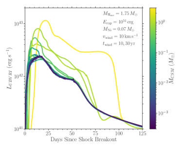
Figure 8: Subset of MESA+STELLA pseudobolometric CSM light-curve models with the single wind velocity ($v_{\rm wind}$) and two different mass-loss duration ($t_{\rm wind}$), color coded by the CSM mass ($M_{\rm CSM}=\dot{M}_{\rm wind}t_{\rm wind}$). Light curves with the same color come from different combinations of $\dot{M}_{\rm wind}$ and $t_{\rm wind}$ that result in the same $M_{\rm CSM}$; higher $\dot{M}_{\rm wind}$ and lower $t_{\rm wind}$ result in sharper light-curve peaks. Note the effect of CSM interaction on both the luminosity and shape.

Figure 9: Similar to Figure 7, but with the CSM models. The early ($\lesssim 10$ days) excess emission are reasonably well reproduced. Note the inferred smaller $E_{\rm exp}$ compared to the CSM-free fits in general, and the large $M_{\rm CSM}$ that suggest violent mass loss in the last few decades before the explosion (actual $M_{\rm CSM}$ could be even higher as the light-curve peaks are lower limits).

In order to account for the early excess emission, we propose CSM interaction as a possible power source, as suggested in $\S$4.2. At handoff to STELLA, we affix a wind density profile with $\rho_{\mathrm{wind}}(r)=\dot{M}_{\mathrm{wind}}/4\pi r^{2}v_{\mathrm{wind}}$, where $\dot{M}_{\mathrm{wind}}$ is a constant wind mass-loss rate, and $v_{\mathrm{wind}}$ is the wind velocity for time $t_{\mathrm{wind}}$ (i.e., the CSM mass, $M_{\mathrm{CSM}}=\dot{M}_{\mathrm{wind}}t_{\mathrm{wind}}$), onto the subset of MESA explosion models that result in short-plateau SNe (40 models each with $M_{\rm Ni}=0.04$, $0.07$, and $0.1\,M_{\odot}$; Figures 5(c), 15(c), and 16(c)). In addition to the 400 spatial zones for the original SN ejecta, we use 200 spatial zones for the CSM model in STELLA. We construct a grid of CSM models by varying $\dot{M}_{\mathrm{wind}}$ ($10^{-5}$–$10^{-1}\,M_{\odot}$ yr^-1 with $0.5$ dex increments) and $t_{\mathrm{wind}}$ ($10$ and $30$ yr) for each MESA short-plateau SN model, assuming a typical RSG $v_{\mathrm{wind}}=10$ km s^-1 (Moriya et al. 2011). The subset of the CSM light-curve model grid is shown in Figure 8 where the effect of increasing CSM mass on the light-curve luminosity and shape can be seen.

In Figure 9, we show the CSM model-grid log likelihood distributions of $M_{\mathrm{CSM}}$ and $E_{\rm exp}$ from $\chi^{2}$ fitting on SNe 2006Y, 2006ai, and 2016egz. The observed early excess emission as well as the overall light curves of SNe 2006Y, 2006ai, and 2016egz are reasonably well reproduced by the CSM models with $M_{\rm CSM}\simeq 0.1$–$0.3\,M_{\odot}$ ($\dot{M}_{\mathrm{wind}}\simeq 10^{-2}\,M_{\odot}$ yr^-1 with $t_{\rm wind}=10$ yr for SN 2006Y and $30$ yr for SNe 2006ai and 2016egz) and $E_{\rm exp}\simeq 1.0$–$1.4\times 10^{51}$ erg. This suggests enhanced mass loss (a few orders of magnitude greater than the standard continuous $\dot{M}_{\rm wind}\sim 10^{-5}\,M_{\odot}\,{\rm yr}^{-1}$) in the last few decades before the explosion. The inferred $E_{\rm exp}$ are generally lower than those from the CSM-free fits (Figure 7) since the CSM interaction provides additional luminosity, especially around the peak. The actual CSM could be even denser and more confined for SNe 2006Y, 2006ai, and 2016egz because their light-curve peaks are lower limits.

4.5 Photospheric Spectra

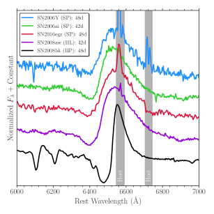
Figure 10: Comparison of the H$\alpha$ P Cygni profiles of short-plateau (SP) SNe 2006Y, 2006ai and 2016egz with the SN IIL 2008aw and the SN IIP 2008bk around $50$ days after explosion (Gutiérrez et al., 2014; Gutiérrez et al., 2017a), retrieved via the Open Supernova Catalog. The gray shaded regions represent host galaxy contamination. Each spectrum is normalized by its broad SN H$\alpha$ peak. Note that the H$\alpha$ P Cygni absorption to emission ratios of SNe 2006Y, 2006ai and 2016egz are smaller than those of the SN IIP 2008bk and even the SN IIL 2008aw.

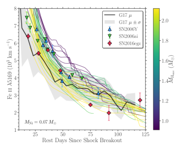
Figure 11: Comparison of Fe ii $\lambda$5169 velocities of SNe 2006Y, 2006ai, and 2016egz with the Gutiérrez et al. (2017a, G17) mean velocity evolution (black line and gray shaded region) and MESA+STELLA short-plateau SN models with $M_{\rm Ni}=0.07\,M_{\odot}$ (defined by the Sobolev optical depth $\tau_{\rm Sob}=1$), color coded by $M_{\rm H_{\rm env}}$ as in Figure 5(c). Error bars denote $1\sigma$ uncertainties and are sometimes smaller than the marker size. Velocity models with the same color come from the same progenitor model exploded with different energies; higher explosion energies result in faster velocities. Note the better agreements with the higher $M_{\rm H_{\rm env}}$ models for SNe 2006Y, 2006ai, and 2016egz.

As in the Anderson et al. (2014) sample light-curve analysis, Gutiérrez et al. (2014); Gutiérrez et al. (2017a, b) also include SNe 2006Y and 2006ai in their sample spectral analysis and identify their spectral peculiarity, namely, the smallest H$\alpha$ P Cygni absorption to emission ratios ($a/e$). They also find a correlation between $a/e$ and light-curve plateau slope (i.e., SNe IIL have shallower absorption components than SNe IIP). Several possible explanations for the smaller $a/e$ for SNe IIL have been proposed, e.g., lower $M_{\rm H_{\rm env}}$ (Schlegel, 1996; Gutiérrez et al., 2014; Gutiérrez et al., 2017b) and steeper envelope density gradients (Dessart & Hillier, 2005; Dessart et al., 2013; Gutiérrez et al., 2014). In Figure 10, we show the H$\alpha$ P Cygni profile comparison of SNe 2006Y, 2006ai, and 2016egz with SNe IIL and IIP. SN 2016egz displays a H$\alpha$ P Cygni profile similar to that of SNe 2006Y and 2006ai with a shallower absorption feature than SNe IIL and IIP. This supports lower $M_{\rm H_{\rm env}}$ as a possible cause of smaller $a/e$ since short-plateau SNe with lower $M_{\rm H_{\rm env}}$ result in smaller $a/e$ than SNe IIP and IIL, as seen in our MESA+STELLA light-curve model grid (Figure 5).

For SNe 2006Y, 2006ai, and 2016egz, we measure expansion velocities of Fe ii $\lambda$5169 from the absorption minimum by fitting a P Cygni profile. In Figure 11, we show the velocity comparison of SNe 2006Y, 2006ai, and 2016egz with the MESA+STELLA short-plateau SN models with $M_{\rm Ni}=0.07\,M_{\odot}$ (Figure 5(c)), as well as the mean velocity evolution from the Gutiérrez et al. (2017a) SN II sample. The overall velocity evolution is better reproduced with the higher $M_{\rm H_{\rm env}}$ ($\gtrsim 1.7\,M_{\odot}$) models. This is in agreement with the values inferred from the light-curve fitting (Figure 7). The Fe ii $\lambda$5169 velocities of SNe 2006Y, 2006ai, and 2016egz are generally higher than the Gutiérrez et al. (2017a) mean velocity evolution, but still within $1\sigma$ deviation. Thus, unlike their light curves, their velocities do not appear to be outliers.

However, it is worth noting that the velocity of SN 2016egz is lower than those of SNe 2006Y and 2006ai, despite it exhibiting a more luminous light curve (Figure 4). This is in disagreement with the SN IIP luminosity–velocity correlation ($L_{P}\propto v_{P}^{2}$) from the homologously expanding photosphere set by H-recombination (Hamuy & Pinto, 2002; Kasen & Woosley, 2009; Goldberg et al., 2019). By comparing the light curves (Figure 5(c)) and velocities (Figure 11) of short-plateau SN models, we do not see an obvious $L_{P}$–$v_{P}$ correlation (e.g., some of the highest and lowest $M_{\rm H_{\rm env}}$ models have similar $L_{P}$, but the highest $M_{\rm H_{\rm env}}$ models have systematically lower $v_{P}$). This suggests that the short-plateau light curves are not purely powered by shock energy released at the H-recombination front; ⁵⁶Ni heating is also important in shaping their light curves (more so than in typical SN IIP light curves). This is in agreement with the light-curve analysis with varying $M_{\rm Ni}$ (Figure 6(c)).

Finally, we note that both line shape and velocity could also be affected by the extra emission from persistent CSM interaction (e.g, Moriya et al. 2011, 2018; Dessart et al. 2016a; Hillier & Dessart 2019), even though high-velocity H$\alpha$ absorption features are absent (Chugai et al., 2007). Thus, the qualitative analyses, partially based on the light-curve modeling, in this section merit future spectral modeling of short-plateau SNe with and without CSM interaction.

4.6 Nebular Spectra

While there are no late-time ($>100$ d) spectra available for SNe 2006Y and 2006ai, we obtained two nebular-phase ($>200$ d) spectra for SN 2016egz (Figure 2). We simultaneously fit a Gaussian profile to the broad SN H$\alpha$ (excluding the narrow host H$\alpha$ region) and a double-Gaussian profile to [O i] $\lambda\lambda 6300,6364$ assuming a doublet flux ratio of 3:1 (as not resolved) and single full width at half-maximum (FWHM) velocity. Due to the low signal-to-noise ratio (S/N) and fringing, we are unable to measure [Ca ii] $\lambda\lambda 7291,7323$ fluxes. Instead, we inject a double-Gaussian profile at the [Ca ii] rest wavelengths by assuming a doublet flux ratio of 1:1 and the same single FWHM velocity as the [O i] doublet at each epoch to place a $3\sigma$ flux upper limit. The measured nebular line fluxes and FWHM velocities are summarized in Tables 3 and 4.

Table 3: SN 2016egz Nebular Line Fluxes ($10^{-15}$ erg s^-1 cm^-2)

Days	[O i] $\lambda\lambda 6300,6364$	H$\alpha$	[Ca ii] $\lambda\lambda 7291,7323$
$278.7$	$2.1\pm 0.4$	$2.6\pm 0.3$	$\leq 2.9$
$309.9$	$2.0\pm 0.3$	$1.8\pm 0.2$	$\leq 2.4$

Table 4: SN 2016egz Nebular FWHM Velocities ($10^{3}$ km s^-1)

Days	[O i] $\lambda\lambda 6300,6364$	H$\alpha$	[Ca ii] $\lambda\lambda 7291,7323$
$278.7$	$3.7\pm 0.6$	$4.0\pm 0.5$	–
$309.9$	$3.4\pm 0.4$	$3.0\pm 0.4$	–

It is known that [O i] and its ratio to [Ca ii] are insensitive respectively to the SN explosive nucleosynthesis and the SN ejecta density and temperature, so can be used as a proxy for progenitor O-core mass, and so ZAMS mass (e.g., Fransson & Chevalier 1989; Woosley & Weaver 1995; Woosley et al. 2002; Elmhamdi et al. 2004; Maeda et al. 2007; Dessart & Hillier 2011, 2020; Jerkstrand et al. 2012, 2014, 2015; Fang & Maeda 2018; Fang et al. 2019). Also, since H$\alpha$ and [N ii] are dominantly emitted respectively from the H- and He-rich envelopes, (H$\alpha$, [N ii])/[O i] can be used as a proxy for H/He-rich envelope stripping (Jerkstrand et al., 2015; Fang et al., 2019; Dessart & Hillier, 2020).

However, there are a few caveats to note especially for stripped-envelope SNe (SESNe: IIb, Ib, and Ic in descending order of H/He-rich envelope mass). [N ii]/[O i] could be affected by the progenitor He burning due to more He/N-layer burning in more massive stars (Jerkstrand et al., 2015; Fang et al., 2019). Also, [Ca ii]/[O i] could be affected by the explosion energy due to more emission from the synthesized calcium than primordial calcium in the H-rich envelope (Li & McCray, 1993; Maguire et al., 2012; Jerkstrand et al., 2015; Jerkstrand, 2017). In principle, the progenitor convective mixing and SN explosive ⁵⁶Ni mixing could also alter these line ratios for CCSNe in general (Jerkstrand, 2017; Dessart & Hillier, 2020). Because of these possible systematic effects, the direct and quantitative comparison of the nature of the progenitors between different subclasses (e.g., SNe II vs. SESNe) will require detailed spectral modeling. Nevertheless, these line ratios should provide rough CCSN progenitor estimates.

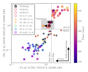
Figure 12: Comparison of the nebular line ratios of SN 2016egz (Table 3) with a CCSN sample, color coded by the phase. [Ca ii]/[O i] and (H$\alpha$, [N ii])/[O i] are proxies for progenitor O-core mass and H/He-rich envelope stripping, respectively. The vertical gray dashed line ($=1.43$) is a rough division between SNe II and SESNe adopted in Gutiérrez et al. (2020), and the horizontal gray dashed line ($=0.71$) is the highest value ($+1\sigma$ error) in the SESN sample of Fang et al. (2019). Note the similar transitional nature of SN 2016egz to SNe II 2015bs and 2017ivv in between SNe II and SESNe (gray shaded region). Figure adapted from Kuncarayakti et al. (2015), Fang et al. (2019), and Gutiérrez et al. (2020), and expanded to include additional measurements from this work on the Kuncarayakti et al. (2015) SN II sample and SNe II 1990E, 1993K, 2012A (Silverman et al., 2017), 1990K (Cappellaro et al., 1995), 1994N (Pastorello et al., 2004), 2002hh (Faran et al., 2014), 2003B, 2008bk (Gutiérrez et al., 2017a), 2005cs (Pastorello et al., 2009), 2012aw (Jerkstrand et al., 2014), 2013ej (Silverman et al., 2012), 2015bs (Anderson et al., 2018), and 2016bkv (Hosseinzadeh et al., 2018), retrieved via the Open Supernova Catalog and WISeREP.

Figure 13: Comparison of the nebular spectra of SN 2016egz with the SN II and IIb models from different progenitor $M_{\rm ZAMS}$. The host spectrum is added to the model spectra that are scaled to match the distance, ⁵⁶Ni mass, and phase of the observed SN spectra. Due to the significant host contamination and low S/N, only broad [O i] and H$\alpha$ features can be identified. Note the observed broad H$\alpha$ and [O i] strengths in between those of SNe II–IIb and $17$–$25\,M_{\odot}$ models, respectively.

In Figure 12, we show the comparison of the nebular line ratios of SN 2016egz with a combined CCSN sample from Kuncarayakti et al. (2015), Fang et al. (2019), and Gutiérrez et al. (2020) and additional SN II measurements from this work. The general increasing and decreasing trends, respectively, in the progenitor O-core mass and H/He-rich envelope stripping can be seen in the sequence of SNe II–IIb–Ib–Ic–IcBL. For a given CCSN, [Ca ii]/[O i] is relatively constant over $\sim 150$–$400$ d after the explosion (Elmhamdi et al., 2004; Maguire et al., 2012; Kuncarayakti et al., 2015; Fang et al., 2019), while (H$\alpha$, [N ii])/[O i] decreases with time (Maguire et al., 2012; Fang et al., 2019). Since the mean phases of the SN II and SESN samples are $330$ days and $215$ days, respectively, we expect to see more separation in the (H$\alpha$, [N ii])/[O i] space if they had been all taken at the same epoch.

Fang et al. (2019) divide the SN IIb sample into extended (eIIb) and compact (cIIb) H-rich envelope classes based on their light-curve morphology. Chevalier & Soderberg 2010 suggest $M_{\rm H_{\rm env}}\gtrsim 0.1\,M_{\odot}$ for SNe eIIb, and otherwise for SNe cIIb. Given the $M_{\rm H_{\rm env}}$ range, SNe eIIb typically result in a double-peak light curve (Figure 5(d)) where the first and second peaks are powered by shock-cooling envelope and radioactive decay, respectively. Compared to the other SESN types, Fang & Maeda (2018) and Fang et al. (2019) identify excess emission around [N ii] for SNe eIIb and attribute it to H$\alpha$ from the residual envelope.

We note that SN 2016egz as well as SNe 2015bs and 2017ivv lie in a somewhat transitional region between SNe II and eIIb–Ib (Figure 12). For SN II 2015bs, Anderson et al. (2018) infer a high progenitor $M_{\rm ZAMS}$ of $17$–$25\,M_{\odot}$ based on the nebular line fluxes and velocities. Dessart & Hillier (2020) also suggest a high $M_{\rm He_{\rm core}}$ and low $M_{\rm H_{\rm env}}$ to better match the broad nebular line profiles ($v_{{\rm H}\alpha,\,{\rm FWHM}}\simeq 4200$ km s^-1; see also Dessart et al. 2010). For SN 2017ivv, Gutiérrez et al. (2020) estimate a $M_{\rm ZAMS}$ of $15$–$17\,M_{\odot}$ and note the transitional characteristics from SN II to IIb by analyzing the temporal evolution of the nebular line ratios. Following this line of reasoning, the nebular line ratios (and upper limits) and velocities of SN 2016egz likely suggest a similar partially stripped massive progenitor. This agrees with the inferred parameters from the light-curve analysis.

In order to be more quantitative, we compare the nebular spectra of SN 2016egz with the SNe II and IIb models of Jerkstrand et al. (2014, 2015), respectively, in Figure 13 where [O i] fluxes can be used to estimate the progenitor $M_{\rm ZAMS}$. We scale the model spectra by the observed distance, ⁵⁶Ni mass, and phase of the SN 2016egz nebular spectra according to Equation (2) of Bostroem et al. (2019). Then, we add the observed host galaxy spectrum to the model spectra to account for the host contamination. The broad SN H$\alpha$ (excluding the narrow host component) fluxes are in between those of the SNe II and IIb models, indicating a small $M_{\rm H_{\rm env}}$. The model [O i] lines start to saturate above $19\,M_{\odot}$ around $300$ days (Jerkstrand et al., 2014), making the $19\,M_{\odot}$ and $25\,M_{\odot}$ models almost indistinguishable. Thus, we put a conservative $M_{\rm ZAMS}$ constraint of $17$–$25\,M_{\odot}$ based on the observed [O i] fluxes. This is consistent with the expected $M_{\rm ZAMS}\gtrsim 17.5\,M_{\odot}$ from the light-curve analysis. One caveat to note is that there is no measurable [O i] $\lambda 5577$ in the observed spectra due to the significant host contamination, preventing us from constraining the temperature and directly estimate the O-core mass (Jerkstrand et al., 2014, 2015; Jerkstrand, 2017).

5 Discussion

5.1 Formation Channel

The short-plateau SNe 2006Y, 2006ai, and 2016egz most likely come from partially stripped massive progenitors, but a remaining question is their exact formation channel. If it is single-star evolution as assumed in this work, the main theoretical uncertainties are RSG wind mass-loss rates and stellar rotation (e.g., Hirschi et al. 2004; Georgy 2012; Chieffi & Limongi 2013; Meynet et al. 2015; Renzo et al. 2017). We assume no rotation and tweak the wind efficiency by hand, but it is debatable whether such high mass-loss rates are physically plausible. Observationally, there is indeed a wide range of measured RSG wind mass-loss rates (e.g., de Jager et al. 1988; van Loon et al. 2005; Mauron & Josselin 2011; Goldman et al. 2017; Beasor et al. 2020). In addition, recent observational and theoretical studies on RSGs and SNe II indicate that RSG wind mass-loss rates may be independent from metallicity (Goldman et al., 2017; Chun et al., 2018; Gutiérrez et al., 2018). Thus, it could be possible that the short-plateau SNe 2006Y, 2006ai, and 2016egz originate from single-star evolution. However, it is unlikely the case if RSG mass-loss rates are metallicity dependent (as in the main-sequence O/B stars; e.g., Vink et al. 2000, 2001; Mokiem et al. 2007), given the estimated subsolar host metallicities (Table 2). In such a case, interacting binary evolution is more plausible, as Eldridge et al. (2017, 2018) indeed show some interacting binary products also result in short-plateau SNe. It is also important to note that any mass-loss models need to reproduce the observed populations of not only SNe II but also RSGs. For example, Neugent et al. (2020) recently show that the luminosity function of RSGs can be used to constrain their mass-loss rates. Future statistical studies with both RSG and SN II populations at various metallicities are required to distinguish the formation channels of short-plateau SNe.

Aside from the continuous mass loss, the origin of the confined dense CSM is not well understood. In the single-star scenario, a number of possible mechanisms have been proposed, including pulsation-driven superwinds (Heger et al., 1997; Yoon & Cantiello, 2010), extended stellar envelopes (Dessart et al., 2017; Soker, 2021), and internal gravity waves (Quataert & Shiode, 2012; Shiode & Quataert, 2014; Quataert et al., 2016; Fuller, 2017; Leung & Fuller, 2020; Morozova et al., 2020; Wu & Fuller, 2021). Although the expected $M_{\rm ZAMS}$ range ($19$–$25\,M_{\odot}$), where pulsation-driven superwinds could significantly alter mass loss, matches with our inferred $M_{\rm ZAMS}$ range for SNe 2006Y, 2006ai, and 2016egz, the expected maximum mass-loss rate of $\lesssim 10^{-3}\,M_{\odot}\,{\rm yr}^{-1}$ around $10^{4}$–$10^{6}$ yr before the core collapse may not result in confined CSM. Also, as the expected timescale of dominant CSM emission from an extended envelope (up to about $10$–$100$ stellar radii) is only over a few days after explosion, whether it can reproduce the $\sim 10$ d excess emission seen in SNe 2006Y, 2006ai, and 2016egz is questionable. In the binary scenario, the confined dense CSM may be expected from a wind collision interface formed between each binary component if the separation is wide enough (Kochanek, 2019). With such a wide separation, however, short-plateau SNe do not result solely from binary interaction (Eldridge et al., 2017, 2018). As such, the enhanced mass loss from internal gravity waves remains more probable, although the light-curve model predictions can be quite flexible by varying the amount and time of nuclear energy injection (Morozova et al., 2020).

5.2 Implications for the RSG Problem

Figure 14: Distribution of the SN II OPTd with a mean $\mu\simeq 86$ days and standard deviation $\sigma\simeq 14$ days. SNe 2006Y, 2006ai, and 2016egz show similar luminous short-plateau light curves, while SNe 2008bp and 2008bu show IIL-like light curves (the extinction and explosion epoch of SN 1992af are not well constrained, and the fall from the plateau of SN 2009ao is not well sampled). Note the small fraction of short-plateau SNe ($3/78\simeq 4\%$).

Regardless of the exact progenitor formation scenario, our conclusion based on the SN photometric and spectroscopic analyses should still hold, and it is worth discussing the implications of the short-plateau SNe for the RSG problem. Some proposed solutions even point toward the nonexistence of the RSG problem, as the high-mass progenitors ($\gtrsim 20\,M_{\odot}$) may not end their lives as RSGs, but as yellow supergiants (or even blue supergiants or Wolf–Rayet stars) resulting in SNe IIb/Ib (or Ib/c) due to binary interaction (Eldridge et al., 2008, 2013, 2017, 2018), stellar rotation (Hirschi et al., 2004; Chieffi & Limongi, 2013), and/or wind mass loss (Georgy, 2012; Meynet et al., 2015; Renzo et al., 2017). Others propose the high-mass RSGs do explode as SNe II, but the mistreatment of dust extinction (Walmswell & Eldridge, 2012; Beasor & Davies, 2016) and/or bolometric correction (Davies & Beasor, 2018) in the direct progenitor identifications systematically underestimates the progenitor masses. In addition, the statistical significance of the RSG problem has been questioned (see Davies & Beasor 2020; Kochanek 2020 for recent discussions). If the RSG problem is indeed real, then the direct collapse of high-mass RSGs to black holes (i.e., failed explosion) is a plausible solution (O’Connor & Ott, 2011; Ugliano et al., 2012; Kochanek, 2014; Gerke et al., 2015; Pejcha & Thompson, 2015; Sukhbold et al., 2016; Adams et al., 2017; Basinger et al., 2020; Pejcha, 2020; Kresse et al., 2021). In this context, the transitional nature of SNe 2006Y, 2006ai, and 2016egz is important, highlighting the possibility that these partially stripped massive progenitors die as RSGs and explode as short-plateau SNe II, rather than becoming SESNe or directly collapsing to black holes.

As a first-order rate estimate for short-plateau SNe, we use the optically thick phase duration (OPTd; the time between the explosion and the plateau drop) distribution of SNe II (including SNe 2006Y, 2006ai, and 2016egz) from Gutiérrez et al. (2018) in Figure 14. The lack of SNe II with ${\rm OPTd}\lesssim 40$ days indicates that there exists an H-rich envelope boundary between SNe II and IIb, as also seen in the light-curve model grid (Figure 5). On the tail of the smooth Gaussian-like OPTd distribution, there is a small population with shorter OPTd than SN 2016egz (Figure 14). SNe 2008bp and 2008bu show IIL-like light curves with fainter ⁵⁶Co decay tails than those of SNe 2006Y, 2006ai, and 2016egz. Their light curves might be reproduced with the high-mass ($\geq 17.5\,M_{\odot}$) progenitor models within the short-plateau $M_{\rm H_{\rm env}}$ range with a lower $M_{\rm Ni}$ and varying $E_{\rm exp}$ (Figures 5(c) and 6(c)). We do not consider the other SNe as probable short-plateau candidates here because of the uncertainties in extinction and explosion epoch for SN 1992af (Anderson et al., 2014; Galbany et al., 2016b; Gutiérrez et al., 2017a) and the poor light-curve sampling at the plateau fall for SN 2009ao. If we take the short-plateau SN fraction of $3/78$ (or $5/78$ if we naively include SNe 2008bp and 2008bu) at face value, a short-plateau SN rate of $\sim 4\%$ (or $\sim 6\%$) of all SNe II can be inferred. This is roughly consistent with the rate estimate from Eldridge et al. (2018) ($\sim 4.7\%$; see $\S$4.3). Recently, Gofman et al. (2020) apply enhanced mass-loss rates to RSGs and found that massive RSGs ($M_{\rm ZAMS}\simeq 20$–$21\,M_{\odot}$) with a similar $M_{\rm H_{\rm env}}$ range ($\sim 0.8$–$1.8\,M_{\odot}$) to that of our short-plateau SN models end up as dust-unobscured SNe II. They roughly estimate a rate of this class to be $2$–$4\%$ of all SNe II, which is similar to our estimate of short-plateau SNe.

Assuming the Salpeter IMF with lower and upper RSG mass limits of $8$ and $25\,M_{\odot}$, respectively, the inferred ZAMS mass range of the short-plateau SNe 2006Y, 2006ai, and 2016egz ($18$–$22\,M_{\odot}$) corresponds to $10\%$ of all SNe II. It may be possible that the missing fraction ($10\%-4\%=6\%$) does not end up as RSGs, but there also seems to be an absence of promising high-mass SESN candidates (Lyman et al., 2016; Taddia et al., 2018; Barbarino et al., 2020). Thus, together with SN 2015bs (Anderson et al., 2018) and the possible failed explosion of a $\sim 25\,M_{\odot}$ RSG (Gerke et al., 2015; Adams et al., 2017; Basinger et al., 2020), this apparent rate mismatch may support the proposed islands of explodability in a sea of black hole formation (Sukhbold et al., 2016) where there is no single mass cut between SN II explosions and black hole formations (see also O’Connor & Ott 2011; Ugliano et al. 2012; Pejcha & Thompson 2015; Patton & Sukhbold 2020; Pejcha 2020; Sukhbold & Adams 2020; Kresse et al. 2021).

In order to further test the hypothesis, more detailed progenitor mass and rate calculations of short-plateau SNe are necessary. The bare photospheres of the short-plateau SN progenitor models in this work lie in the effective temperature and photospheric luminosity ranges of $3.65<{\rm log}_{10}(T_{\rm eff}/{\rm K})<3.72$ and $5.23<{\rm log}_{10}(L_{\rm ph}/L_{\odot})<5.53$, respectively, which are within those observed for luminous RSGs (e.g., Levesque et al. 2005, 2006; Massey et al. 2009; Drout et al. 2012; Gordon et al. 2016). Given the high constant mass loss as well as the enhanced mass loss in the last few decades before the explosion, however, significant dust extinction is likely expected for the short-plateau SN progenitors (e.g., Nozawa & Fukugita 2013; Nozawa et al. 2014), making their direct progenitor identifications unlikely (if they all come from the single-star channel; see Eldridge et al. 2017, 2018 for the interacting binary channel). The circumstellar dust is likely destroyed as the SN shock progresses through. Therefore, SN photometric and spectroscopic analyses of large samples will be required to better determine their progenitor mass and rate distributions.

6 Conclusions

We have presented the optical/NIR photometric and spectroscopic observations of luminous Type II short-plateau SNe 2006Y, 2006ai, and 2016egz. Based on the V-band and pseudobolometric light-curve sample comparisons, the peculiar light curves with the short plateaus and luminous peaks suggest partially stripped H-rich envelopes and CSM interaction at early time. We have constructed a large MESA+STELLA single-star progenitor and light-curve model grid (with and without CSM interaction) that shows a continuous population of SNe IIP–IIL–IIb-like light-curve morphology in descending order of H-rich envelope mass, with short-plateau SNe lying in a confined parameter space between SNe IIL and IIb with large ⁵⁶Ni masses ($\gtrsim 0.05\,M_{\odot}$). For SNe 2006Y, 2006ai, and 2016egz, our model grid suggests high-mass RSG progenitors ($M_{\rm ZAMS}\simeq 18$–$22\,M_{\odot}$) with small H-rich envelope masses ($M_{\rm H_{\rm env}}\simeq 1.7\,M_{\odot}$) to reproduce the short-plateau light curves, and enhanced mass loss ($\dot{M}\simeq 10^{-2}\,M_{\odot}\,{\rm yr}^{-1}$) for the last few decades before the explosion to capture the early luminous peaks. In addition, the P Cygni profiles and photospheric velocities likely point toward low H-rich envelope masses, and the nebular line ratios and spectral model comparisons prefer high-mass ($M_{\rm ZAMS}\simeq 17$–$25\,M_{\odot}$) progenitors.

Although the exact progenitor formation channel remains an open question, the transitional nature of SNe 2006Y, 2006ai, and 2016egz has important implications for the RSG problem, in that these partially stripped massive progenitors end their lives as RSGs and explode as short-plateau SNe. We roughly estimate a short-plateau SN rate of $\sim 4\%$ of all SNe II, which is smaller than the IMF expectation of $\sim 10\%$. This rate mismatch may support the proposed islands of explodability scenario. Further verification of this scenario requires the determination of the short-plateau SN progenitor mass and rate distributions through large SN photometric and spectroscopic sample analyses (as done in this work for three objects), as their direct progenitor identifications are expected to be quite challenging. Current and future large transient surveys are promising to provide the necessary SN samples.

Appendix A Extra MESA+STELLA Description and Models

We start with MESA revision 10398 test suites, example_make_pre_ccsn and example_ccsn_IIp, respectively, for progenitor evolution from the pre-main sequence to Fe-core infall and SN explosions from the core collapse to near shock breakout (by excising the core and injecting a thermal bomb). Then we use STELLA for SN light-curve and expansion-velocity calculations from the shock breakout to radioactive decay tail. The reader is referred to Paxton et al. (2018) for more details on the workflow and relevant physical parameters.

For the MESA progenitor model grid, we vary ZAMS masses ($M_{\rm ZAMS}=10.0$–$25.0\,M_{\odot}$ with $2.5\,M_{\odot}$ increments) and wind scaling factors ($\eta_{\rm wind}=0.0$–$3.0$ with $0.1$ increments), while fixing subsolar ZAMS metallicity ($Z=0.3\,Z_{\odot}$), no rotation ($\nu/\nu_{\rm crit}=0$), mixing length in the H-rich envelope ($\alpha_{\rm env}=3.0$), and convective overshooting parameters ($f_{\rm ov}=0.02$ and $0.01$ for $10.0\,M_{\odot}$ and the other ZAMS masses, respectively). As the main objective of this work is to observe how SN II light curves are affected by H-rich envelope stripping, we control the progenitor mass loss by using the Dutch prescription (Glebbeek et al. 2009, and references therein) and arbitrarily varying $\eta_{\rm wind}$ in single-star evolution (see, e.g., Mauron & Josselin 2011; Goldman et al. 2017; Beasor et al. 2020 for a wide range of observed RSG mass-loss rates), rather than exploring the details of mass-loss mechanisms (e.g., interacting binary evolution; see Eldridge 2017 for a review). With our parameter setup, $\sim 20\%$ of the MESA progenitor models do not advance to Fe-core formation, mostly due to some low-mass ($\leq 12.5\,M_{\odot}$) models developing highly degenerate cores and fail during off-center burning stages such as neon ignition.

For the MESA explosion model grid, we vary explosion energies ($E_{\rm exp}=0.4$–$2.0\times 10^{51}$ erg with $0.2\times 10^{51}$ erg increments) for each progenitor model. The SN shock propagation is modeled with the Duffell (2016) Rayleigh-Taylor instability mixing prescription until near shock breakout, and the resultant ⁵⁶Ni distribution is scaled to match a fixed ⁵⁶Ni mass ($M_{\rm Ni}=0.04$, $0.07$, and $0.1\,M_{\odot}$). Then, we hand off these explosion models to STELLA to produce synthetic light curves and expansion velocities using 400 spatial zones and 40 frequency bins. Any fallback material is frozen onto the central remnant and excised via a $500$ km s^-1 velocity cut at the inner boundary at the handoff between MESA and STELLA (i.e., the extra heating from fallback accretion onto the central remnant is not taken into account, but can be relevant for high-mass progenitors with low $E_{\rm exp}$; e.g., Lisakov et al. 2018; Chan et al. 2018; Moriya et al. 2019). With our parameter setup, $\sim 5\%$ each of the MESA explosion models and STELLA light-curve models do not converge numerically, mostly with high-mass ($\geq 22.5\,M_{\odot}$) progenitors. We simply discard the failed models (in Fe-core formation or explosion) and focus on the bulk properties of the model grid in this work.

As for the model grids with $M_{\rm Ni}=0.04$ and $0.1\,M_{\odot}$, the light-curve models are shown in Figures 15 and 16, and the short-plateau SN velocity models are shown in Figure 17.

Figure 15: Same as Figure 5, but with $M_{\rm Ni}=0.04\,M_{\odot}$.

Figure 16: Same as Figure 5, but with $M_{\rm Ni}=0.1\,M_{\odot}$.

Figure 17: Same as Figure 11, but with $M_{\rm Ni}=0.04$ and $0.1\,M_{\odot}$.

References

- Adams et al. (2017) Adams, S. M., Kochanek, C. S., Gerke, J. R., Stanek, K. Z., & Dai, X. 2017, MNRAS, 468, 4968
- Aihara et al. (2011) Aihara, H., Allende Prieto, C., An, D., et al. 2011, ApJS, 193, 29
- Albareti et al. (2017) Albareti, F. D., Allende Prieto, C., Almeida, A., et al. 2017, ApJS, 233, 25
- Anderson et al. (2014) Anderson, J. P., González-Gaitán, S., Hamuy, M., et al. 2014, ApJ, 786, 67
- Anderson et al. (2016) Anderson, J. P., Gutiérrez, C. P., Dessart, L., et al. 2016, A&A, 589, A110
- Anderson et al. (2018) Anderson, J. P., Dessart, L., Gutiérrez, C. P., et al. 2018, Nature Astronomy, 2, 574
- Arcavi (2017) Arcavi, I. 2017, Hydrogen-Rich Core-Collapse Supernovae, ed. A. W. Alsabti & P. Murdin (Cham: Springer International Publishing), 239–276
- Arcavi et al. (2012) Arcavi, I., Gal-Yam, A., Cenko, S. B., et al. 2012, ApJ, 756, L30
- Asplund et al. (2009) Asplund, M., Grevesse, N., Sauval, A. J., & Scott, P. 2009, ARA&A, 47, 481
- Astropy Collaboration et al. (2018) Astropy Collaboration, Price-Whelan, A. M., Sipőcz, B. M., et al. 2018, AJ, 156, 123
- Baklanov et al. (2005) Baklanov, P. V., Blinnikov, S. I., & Pavlyuk, N. N. 2005, Astronomy Letters, 31, 429
- Baldwin et al. (1981) Baldwin, J. A., Phillips, M. M., & Terlevich, R. 1981, PASP, 93, 5
- Barbarino et al. (2020) Barbarino, C., Sollerman, J., Taddia, F., et al. 2020, arXiv e-prints, arXiv:2010.08392
- Barbon et al. (1979) Barbon, R., Ciatti, F., & Rosino, L. 1979, A&A, 72, 287
- Basinger et al. (2020) Basinger, C. M., Kochanek, C. S., Adams, S. M., Dai, X., & Stanek, K. Z. 2020, arXiv e-prints, arXiv:2007.15658
- Beasor & Davies (2016) Beasor, E. R., & Davies, B. 2016, MNRAS, 463, 1269
- Beasor et al. (2020) Beasor, E. R., Davies, B., Smith, N., et al. 2020, MNRAS, 492, 5994
- Bertin & Arnouts (1996) Bertin, E., & Arnouts, S. 1996, A&AS, 117, 393
- Bianco et al. (2016) Bianco, F. B., Modjaz, M., Oh, S. M., et al. 2016, Astronomy and Computing, 16, 54
- Blinnikov et al. (2000) Blinnikov, S., Lundqvist, P., Bartunov, O., Nomoto, K., & Iwamoto, K. 2000, ApJ, 532, 1132
- Blinnikov & Sorokina (2004) Blinnikov, S., & Sorokina, E. 2004, Ap&SS, 290, 13
- Blinnikov et al. (1998) Blinnikov, S. I., Eastman, R., Bartunov, O. S., Popolitov, V. A., & Woosley, S. E. 1998, ApJ, 496, 454
- Blinnikov et al. (2006) Blinnikov, S. I., Röpke, F. K., Sorokina, E. I., et al. 2006, A&A, 453, 229
- Bostroem et al. (2019) Bostroem, K. A., Valenti, S., Horesh, A., et al. 2019, MNRAS, 485, 5120
- Bostroem et al. (2020) Bostroem, K. A., Valenti, S., Sand, D. J., et al. 2020, ApJ, 895, 31
- Brown (2016) Brown, J. 2016, Transient Name Server Discovery Report, 2016-484, 1
- Brown et al. (2013) Brown, T. M., Baliber, N., Bianco, F. B., et al. 2013, PASP, 125, 1031
- Bruch et al. (2021) Bruch, R. J., Gal-Yam, A., Schulze, S., et al. 2021, ApJ, 912, 46
- Cappellaro et al. (1995) Cappellaro, E., Danziger, I. J., della Valle, M., Gouiffes, C., & Turatto, M. 1995, A&A, 293, 723
- Chan et al. (2018) Chan, C., Müller, B., Heger, A., Pakmor, R., & Springel, V. 2018, ApJ, 852, L19
- Chevalier & Soderberg (2010) Chevalier, R. A., & Soderberg, A. M. 2010, ApJ, 711, L40
- Chieffi & Limongi (2013) Chieffi, A., & Limongi, M. 2013, ApJ, 764, 21
- Chugai et al. (2007) Chugai, N. N., Chevalier, R. A., & Utrobin, V. P. 2007, ApJ, 662, 1136
- Chun et al. (2018) Chun, S.-H., Yoon, S.-C., Jung, M.-K., Kim, D. U., & Kim, J. 2018, ApJ, 853, 79
- Colless et al. (2003) Colless, M., Peterson, B. A., Jackson, C., et al. 2003, arXiv e-prints, arXiv:astro-ph/0306581
- Davies & Beasor (2018) Davies, B., & Beasor, E. R. 2018, MNRAS, 474, 2116
- Davies & Beasor (2020) Davies, B., & Beasor, E. R. 2020, MNRAS, 496, L142
- Davis et al. (2019) Davis, S., Hsiao, E. Y., Ashall, C., et al. 2019, ApJ, 887, 4
- de Jager et al. (1988) de Jager, C., Nieuwenhuijzen, H., & van der Hucht, K. A. 1988, A&AS, 72, 259
- Dessart & Hillier (2005) Dessart, L., & Hillier, D. J. 2005, A&A, 437, 667
- Dessart & Hillier (2011) Dessart, L., & Hillier, D. J. 2011, MNRAS, 410, 1739
- Dessart & Hillier (2019) Dessart, L., & Hillier, D. J. 2019, A&A, 625, A9
- Dessart & Hillier (2020) Dessart, L., & Hillier, D. J. 2020, A&A, 642, A33
- Dessart et al. (2016a) Dessart, L., Hillier, D. J., Audit, E., Livne, E., & Waldman, R. 2016a, MNRAS, 458, 2094
- Dessart et al. (2011) Dessart, L., Hillier, D. J., Livne, E., et al. 2011, MNRAS, 414, 2985
- Dessart et al. (2013) Dessart, L., Hillier, D. J., Waldman, R., & Livne, E. 2013, MNRAS, 433, 1745
- Dessart et al. (2016b) Dessart, L., Hillier, D. J., Woosley, S., et al. 2016b, MNRAS, 458, 1618
- Dessart et al. (2017) Dessart, L., John Hillier, D., & Audit, E. 2017, A&A, 605, A83
- Dessart et al. (2010) Dessart, L., Livne, E., & Waldman, R. 2010, MNRAS, 408, 827
- Drout et al. (2012) Drout, M. R., Massey, P., & Meynet, G. 2012, ApJ, 750, 97
- Duffell (2016) Duffell, P. C. 2016, ApJ, 821, 76
- Eisenstein et al. (2011) Eisenstein, D. J., Weinberg, D. H., Agol, E., et al. 2011, AJ, 142, 72
- Eldridge (2017) Eldridge, J. 2017, Population Synthesis of Massive Close Binary Evolution, ed. A. W. Alsabti & P. Murdin (Cham: Springer International Publishing), 1–22
- Eldridge et al. (2013) Eldridge, J. J., Fraser, M., Smartt, S. J., Maund, J. R., & Crockett, R. M. 2013, MNRAS, 436, 774
- Eldridge et al. (2008) Eldridge, J. J., Izzard, R. G., & Tout, C. A. 2008, MNRAS, 384, 1109
- Eldridge et al. (2017) Eldridge, J. J., Stanway, E. R., Xiao, L., et al. 2017, PASA, 34, e058
- Eldridge et al. (2018) Eldridge, J. J., Xiao, L., Stanway, E. R., Rodrigues, N., & Guo, N. Y. 2018, PASA, 35, 49
- Elmhamdi et al. (2004) Elmhamdi, A., Danziger, I. J., Cappellaro, E., et al. 2004, A&A, 426, 963
- Fang & Maeda (2018) Fang, Q., & Maeda, K. 2018, ApJ, 864, 47
- Fang et al. (2019) Fang, Q., Maeda, K., Kuncarayakti, H., Sun, F., & Gal-Yam, A. 2019, Nature Astronomy, 3, 434
- Faran et al. (2014) Faran, T., Poznanski, D., Filippenko, A. V., et al. 2014, MNRAS, 442, 844
- Filippenko (1982) Filippenko, A. V. 1982, PASP, 94, 715
- Fitzpatrick (1999) Fitzpatrick, E. L. 1999, PASP, 111, 63
- Förster et al. (2018) Förster, F., Moriya, T. J., Maureira, J. C., et al. 2018, Nature Astronomy, 2, 808
- Fransson & Chevalier (1989) Fransson, C., & Chevalier, R. A. 1989, ApJ, 343, 323
- Fraser et al. (2016) Fraser, M., Reynolds, T., Inserra, C., & Yaron, O. 2016, Transient Name Server Classification Report, 2016-490, 1
- Fuller (2017) Fuller, J. 2017, MNRAS, 470, 1642
- Gal-Yam et al. (2014) Gal-Yam, A., Arcavi, I., Ofek, E. O., et al. 2014, Nature, 509, 471
- Galbany et al. (2014) Galbany, L., Stanishev, V., Mourão, A. M., et al. 2014, A&A, 572, A38
- Galbany et al. (2016a) Galbany, L., Stanishev, V., Mourão, A. M., et al. 2016a, A&A, 591, A48
- Galbany et al. (2016b) Galbany, L., Hamuy, M., Phillips, M. M., et al. 2016b, AJ, 151, 33
- Georgy (2012) Georgy, C. 2012, A&A, 538, L8
- Gerke et al. (2015) Gerke, J. R., Kochanek, C. S., & Stanek, K. Z. 2015, MNRAS, 450, 3289
- Glebbeek et al. (2009) Glebbeek, E., Gaburov, E., de Mink, S. E., Pols, O. R., & Portegies Zwart, S. F. 2009, A&A, 497, 255
- Gofman et al. (2020) Gofman, R. A., Gluck, N., & Soker, N. 2020, MNRAS, 494, 5230
- Goldberg & Bildsten (2020) Goldberg, J. A., & Bildsten, L. 2020, ApJ, 895, L45
- Goldberg et al. (2019) Goldberg, J. A., Bildsten, L., & Paxton, B. 2019, ApJ, 879, 3
- Goldman et al. (2017) Goldman, S. R., van Loon, J. T., Zijlstra, A. A., et al. 2017, MNRAS, 465, 403
- Gordon et al. (2016) Gordon, M. S., Humphreys, R. M., & Jones, T. J. 2016, ApJ, 825, 50
- Graham (2019) Graham, J. F. 2019, arXiv e-prints, arXiv:1905.13197
- Guevel & Hosseinzadeh (2017) Guevel, D., & Hosseinzadeh, G. 2017, Dguevel/Pyzogy: Initial Release, v0.0.1, Zenodo, doi:10.5281/zenodo.1043973
- Guillochon et al. (2017) Guillochon, J., Parrent, J., Kelley, L. Z., & Margutti, R. 2017, ApJ, 835, 64
- Gutiérrez et al. (2014) Gutiérrez, C. P., Anderson, J. P., Hamuy, M., et al. 2014, ApJ, 786, L15
- Gutiérrez et al. (2017a) Gutiérrez, C. P., Anderson, J. P., Hamuy, M., et al. 2017a, ApJ, 850, 89
- Gutiérrez et al. (2017b) Gutiérrez, C. P., Anderson, J. P., Hamuy, M., et al. 2017b, ApJ, 850, 90
- Gutiérrez et al. (2018) Gutiérrez, C. P., Anderson, J. P., Sullivan, M., et al. 2018, MNRAS, 479, 3232
- Gutiérrez et al. (2020) Gutiérrez, C. P., Pastorello, A., Jerkstrand, A., et al. 2020, MNRAS, 499, 974
- Hamuy (2003) Hamuy, M. 2003, ApJ, 582, 905
- Hamuy & Pinto (2002) Hamuy, M., & Pinto, P. A. 2002, ApJ, 566, L63
- Hamuy et al. (2006) Hamuy, M., Folatelli, G., Morrell, N. I., et al. 2006, PASP, 118, 2
- Heger et al. (2003) Heger, A., Fryer, C. L., Woosley, S. E., Langer, N., & Hartmann, D. H. 2003, ApJ, 591, 288
- Heger et al. (1997) Heger, A., Jeannin, L., Langer, N., & Baraffe, I. 1997, A&A, 327, 224
- Hillier & Dessart (2019) Hillier, D. J., & Dessart, L. 2019, A&A, 631, A8
- Hirschi et al. (2004) Hirschi, R., Meynet, G., & Maeder, A. 2004, A&A, 425, 649
- Hosseinzadeh et al. (2018) Hosseinzadeh, G., Valenti, S., McCully, C., et al. 2018, ApJ, 861, 63
- Hunter (2007) Hunter, J. D. 2007, Computing in Science and Engineering, 9, 90
- Jerkstrand (2017) Jerkstrand, A. 2017, Spectra of Supernovae in the Nebular Phase, ed. A. W. Alsabti & P. Murdin (Cham: Springer International Publishing), 795–842
- Jerkstrand et al. (2015) Jerkstrand, A., Ergon, M., Smartt, S. J., et al. 2015, A&A, 573, A12
- Jerkstrand et al. (2012) Jerkstrand, A., Fransson, C., Maguire, K., et al. 2012, A&A, 546, A28
- Jerkstrand et al. (2014) Jerkstrand, A., Smartt, S. J., Fraser, M., et al. 2014, MNRAS, 439, 3694
- Kasen & Woosley (2009) Kasen, D., & Woosley, S. E. 2009, ApJ, 703, 2205
- Kennicutt (1998) Kennicutt, Robert C., J. 1998, ARA&A, 36, 189
- Kewley et al. (2006) Kewley, L. J., Groves, B., Kauffmann, G., & Heckman, T. 2006, MNRAS, 372, 961
- Khazov et al. (2016) Khazov, D., Yaron, O., Gal-Yam, A., et al. 2016, ApJ, 818, 3
- Kochanek (2014) Kochanek, C. S. 2014, ApJ, 785, 28
- Kochanek (2019) Kochanek, C. S. 2019, MNRAS, 483, 3762
- Kochanek (2020) Kochanek, C. S. 2020, MNRAS, 493, 4945
- Kochanek et al. (2017) Kochanek, C. S., Shappee, B. J., Stanek, K. Z., et al. 2017, PASP, 129, 104502
- Kozyreva et al. (2019) Kozyreva, A., Nakar, E., & Waldman, R. 2019, MNRAS, 483, 1211
- Kresse et al. (2021) Kresse, D., Ertl, T., & Janka, H.-T. 2021, ApJ, 909, 169
- Krisciunas et al. (2017) Krisciunas, K., Contreras, C., Burns, C. R., et al. 2017, AJ, 154, 211
- Kuncarayakti et al. (2015) Kuncarayakti, H., Maeda, K., Bersten, M. C., et al. 2015, A&A, 579, A95
- Landolt (1992) Landolt, A. U. 1992, AJ, 104, 340
- Leung & Fuller (2020) Leung, S.-C., & Fuller, J. 2020, ApJ, 900, 99
- Levesque et al. (2005) Levesque, E. M., Massey, P., Olsen, K. A. G., et al. 2005, ApJ, 628, 973
- Levesque et al. (2006) Levesque, E. M., Massey, P., Olsen, K. A. G., et al. 2006, ApJ, 645, 1102
- Li & McCray (1993) Li, H., & McCray, R. 1993, ApJ, 405, 730
- Lisakov et al. (2018) Lisakov, S. M., Dessart, L., Hillier, D. J., Waldman, R., & Livne, E. 2018, MNRAS, 473, 3863
- Luckas et al. (2006a) Luckas, P., Trondal, O., & Schwartz, M. 2006a, Central Bureau Electronic Telegrams, 406, 1
- Luckas et al. (2006b) Luckas, P., Trondal, O., Schwartz, M., & Subbarao, M. 2006b, IAU Circ., 8668, 2
- Lyman et al. (2016) Lyman, J. D., Bersier, D., James, P. A., et al. 2016, MNRAS, 457, 328
- Maeda et al. (2007) Maeda, K., Kawabata, K., Tanaka, M., et al. 2007, ApJ, 658, L5
- Maguire et al. (2012) Maguire, K., Jerkstrand, A., Smartt, S. J., et al. 2012, MNRAS, 420, 3451
- Massey et al. (2009) Massey, P., Silva, D. R., Levesque, E. M., et al. 2009, ApJ, 703, 420
- Mauron & Josselin (2011) Mauron, N., & Josselin, E. 2011, A&A, 526, A156
- Meynet et al. (2015) Meynet, G., Chomienne, V., Ekström, S., et al. 2015, A&A, 575, A60
- Mokiem et al. (2007) Mokiem, M. R., de Koter, A., Vink, J. S., et al. 2007, A&A, 473, 603
- Moriya et al. (2011) Moriya, T., Tominaga, N., Blinnikov, S. I., Baklanov, P. V., & Sorokina, E. I. 2011, MNRAS, 415, 199
- Moriya et al. (2018) Moriya, T. J., Förster, F., Yoon, S.-C., Gräfener, G., & Blinnikov, S. I. 2018, MNRAS, 476, 2840
- Moriya et al. (2019) Moriya, T. J., Müller, B., Chan, C., Heger, A., & Blinnikov, S. I. 2019, ApJ, 880, 21
- Moriya et al. (2017) Moriya, T. J., Yoon, S.-C., Gräfener, G., & Blinnikov, S. I. 2017, MNRAS, 469, L108
- Morozova et al. (2020) Morozova, V., Piro, A. L., Fuller, J., & Van Dyk, S. D. 2020, ApJ, 891, L32
- Morozova et al. (2015) Morozova, V., Piro, A. L., Renzo, M., et al. 2015, ApJ, 814, 63
- Morozova et al. (2017) Morozova, V., Piro, A. L., & Valenti, S. 2017, ApJ, 838, 28
- Morozova et al. (2018) Morozova, V., Piro, A. L., & Valenti, S. 2018, ApJ, 858, 15
- Morrell & Folatelli (2006) Morrell, N., & Folatelli, G. 2006, Central Bureau Electronic Telegrams, 422, 1
- Nakaoka et al. (2019) Nakaoka, T., Moriya, T. J., Tanaka, M., et al. 2019, ApJ, 875, 76
- Neugent et al. (2020) Neugent, K. F., Massey, P., Georgy, C., et al. 2020, ApJ, 889, 44
- Nomoto et al. (1995) Nomoto, K. I., Iwamoto, K., & Suzuki, T. 1995, Phys. Rep., 256, 173
- Nozawa & Fukugita (2013) Nozawa, T., & Fukugita, M. 2013, ApJ, 770, 27
- Nozawa et al. (2014) Nozawa, T., Yoon, S.-C., Maeda, K., et al. 2014, ApJ, 787, L17
- O’Connor & Ott (2011) O’Connor, E., & Ott, C. D. 2011, ApJ, 730, 70
- Oliphant (2006) Oliphant, T. E. 2006, A Guide to NumPy (USA: Trelgol Publishing)
- Pastorello et al. (2004) Pastorello, A., Zampieri, L., Turatto, M., et al. 2004, MNRAS, 347, 74
- Pastorello et al. (2009) Pastorello, A., Valenti, S., Zampieri, L., et al. 2009, MNRAS, 394, 2266
- Patton & Sukhbold (2020) Patton, R. A., & Sukhbold, T. 2020, MNRAS, 499, 2803
- Paxton et al. (2011) Paxton, B., Bildsten, L., Dotter, A., et al. 2011, ApJS, 192, 3
- Paxton et al. (2013) Paxton, B., Cantiello, M., Arras, P., et al. 2013, ApJS, 208, 4
- Paxton et al. (2015) Paxton, B., Marchant, P., Schwab, J., et al. 2015, ApJS, 220, 15
- Paxton et al. (2018) Paxton, B., Schwab, J., Bauer, E. B., et al. 2018, ApJS, 234, 34
- Paxton et al. (2019) Paxton, B., Smolec, R., Schwab, J., et al. 2019, ApJS, 243, 10
- Pejcha (2020) Pejcha, O. 2020, The Explosion Mechanism of Core-Collapse Supernovae and Its Observational Signatures (Cham: Springer International Publishing), 189–211
- Pejcha & Thompson (2015) Pejcha, O., & Thompson, T. A. 2015, ApJ, 801, 90
- Persson et al. (1998) Persson, S. E., Murphy, D. C., Krzeminski, W., Roth, M., & Rieke, M. J. 1998, AJ, 116, 2475
- Pessi et al. (2019) Pessi, P. J., Folatelli, G., Anderson, J. P., et al. 2019, MNRAS, 488, 4239
- Popov (1993) Popov, D. V. 1993, ApJ, 414, 712
- Quataert et al. (2016) Quataert, E., Fernández, R., Kasen, D., Klion, H., & Paxton, B. 2016, MNRAS, 458, 1214
- Quataert & Shiode (2012) Quataert, E., & Shiode, J. 2012, MNRAS, 423, L92
- Renzo et al. (2017) Renzo, M., Ott, C. D., Shore, S. N., & de Mink, S. E. 2017, A&A, 603, A118
- Salim et al. (2007) Salim, S., Rich, R. M., Charlot, S., et al. 2007, ApJS, 173, 267
- Salpeter (1955) Salpeter, E. E. 1955, ApJ, 121, 161
- Sanders et al. (2015) Sanders, N. E., Soderberg, A. M., Gezari, S., et al. 2015, ApJ, 799, 208
- Schlafly & Finkbeiner (2011) Schlafly, E. F., & Finkbeiner, D. P. 2011, ApJ, 737, 103
- Schlegel (1996) Schlegel, E. M. 1996, AJ, 111, 1660
- Science Software Branch at STScI (2012) Science Software Branch at STScI. 2012, PyRAF: Python alternative for IRAF, ascl:1207.011
- Seibert et al. (2012) Seibert, M., Wyder, T., Neill, J., et al. 2012, in American Astronomical Society Meeting Abstracts, Vol. 219, American Astronomical Society Meeting Abstracts #219, 340.01
- Shappee et al. (2014) Shappee, B. J., Prieto, J. L., Grupe, D., et al. 2014, ApJ, 788, 48
- Shiode & Quataert (2014) Shiode, J. H., & Quataert, E. 2014, ApJ, 780, 96
- Silverman et al. (2012) Silverman, J. M., Foley, R. J., Filippenko, A. V., et al. 2012, MNRAS, 425, 1789
- Silverman et al. (2017) Silverman, J. M., Pickett, S., Wheeler, J. C., et al. 2017, MNRAS, 467, 369
- Smartt (2009) Smartt, S. J. 2009, ARA&A, 47, 63
- Smartt (2015) Smartt, S. J. 2015, PASA, 32, e016
- Smartt et al. (2015) Smartt, S. J., Valenti, S., Fraser, M., et al. 2015, A&A, 579, A40
- Smith et al. (2002) Smith, J. A., Tucker, D. L., Kent, S., et al. 2002, AJ, 123, 2121
- Smith (2017) Smith, N. 2017, Interacting Supernovae: Types IIn and Ibn, ed. A. W. Alsabti & P. Murdin (Cham: Springer International Publishing), 403–429
- Soker (2021) Soker, N. 2021, ApJ, 906, 1
- Stetson (2000) Stetson, P. B. 2000, PASP, 112, 925
- Stritzinger et al. (2011) Stritzinger, M. D., Phillips, M. M., Boldt, L. N., et al. 2011, AJ, 142, 156
- Sukhbold & Adams (2020) Sukhbold, T., & Adams, S. 2020, MNRAS, 492, 2578
- Sukhbold et al. (2016) Sukhbold, T., Ertl, T., Woosley, S. E., Brown, J. M., & Janka, H. T. 2016, ApJ, 821, 38
- Taddia et al. (2018) Taddia, F., Stritzinger, M. D., Bersten, M., et al. 2018, A&A, 609, A136
- Ugliano et al. (2012) Ugliano, M., Janka, H.-T., Marek, A., & Arcones, A. 2012, ApJ, 757, 69
- Valenti et al. (2014) Valenti, S., Sand, D., Pastorello, A., et al. 2014, MNRAS, 438, L101
- Valenti et al. (2015) Valenti, S., Sand, D., Stritzinger, M., et al. 2015, MNRAS, 448, 2608
- Valenti et al. (2016) Valenti, S., Howell, D. A., Stritzinger, M. D., et al. 2016, MNRAS, 459, 3939
- Van Dyk (2016) Van Dyk, S. D. 2016, Supernova Progenitors Observed with HST, ed. A. W. Alsabti & P. Murdin (Cham: Springer International Publishing), 1–27
- van Loon et al. (2005) van Loon, J. T., Cioni, M. R. L., Zijlstra, A. A., & Loup, C. 2005, A&A, 438, 273
- Vink et al. (2000) Vink, J. S., de Koter, A., & Lamers, H. J. G. L. M. 2000, A&A, 362, 295
- Vink et al. (2001) Vink, J. S., de Koter, A., & Lamers, H. J. G. L. M. 2001, A&A, 369, 574
- Virtanen et al. (2020) Virtanen, P., Gommers, R., Oliphant, T. E., et al. 2020, Nature Methods, 17, 261
- Walmswell & Eldridge (2012) Walmswell, J. J., & Eldridge, J. J. 2012, MNRAS, 419, 2054
- Waskom et al. (2020) Waskom, M., Botvinnik, O., Ostblom, J., et al. 2020, mwaskom/seaborn: v0.10.0 (January 2020), v0.10.0, Zenodo, doi:10.5281/zenodo.3629446
- Woosley et al. (2002) Woosley, S. E., Heger, A., & Weaver, T. A. 2002, Reviews of Modern Physics, 74, 1015
- Woosley & Weaver (1995) Woosley, S. E., & Weaver, T. A. 1995, ApJS, 101, 181
- Wu & Fuller (2021) Wu, S., & Fuller, J. 2021, ApJ, 906, 3
- Yaron & Gal-Yam (2012) Yaron, O., & Gal-Yam, A. 2012, PASP, 124, 668
- Yaron et al. (2017) Yaron, O., Perley, D. A., Gal-Yam, A., et al. 2017, Nature Physics, 13, 510
- Yoon & Cantiello (2010) Yoon, S.-C., & Cantiello, M. 2010, ApJ, 717, L62
- Zackay et al. (2016) Zackay, B., Ofek, E. O., & Gal-Yam, A. 2016, ApJ, 830, 27
- Zapartas et al. (2021) Zapartas, E., de Mink, S. E., Justham, S., et al. 2021, A&A, 645, A6
- Zapartas et al. (2019) Zapartas, E., de Mink, S. E., Justham, S., et al. 2019, A&A, 631, A5