Rosella: A Self-Driving Distributed Scheduler for Heterogeneous Clusters

Qiong Wu and Zhenming Liu
William & Mary

Abstract

Large-scale interactive web services and advanced AI applications make sophisticated decisions in real-time, based on executing a massive amount of computation tasks on thousands of servers. Task schedulers, which often operate in heterogeneous and volatile environments, require high throughput, i.e., scheduling millions of tasks per second, and low latency, i.e., incurring minimal scheduling delays for millisecond-level tasks. Scheduling is further complicated by other users’ workloads in a shared system, other background activities, and the diverse hardware configurations inside datacenters.

We present Rosella, a new self-driving, distributed approach for task scheduling in heterogeneous clusters. Rosella automatically learns the compute environment and adjusts its scheduling policy in real-time. The solution provides high throughput and low latency simultaneously because it runs in parallel on multiple machines with minimum coordination and only performs simple operations for each scheduling decision. Our learning module monitors total system load and uses the information to dynamically determine optimal estimation strategy for the backends’ compute-power. Rosella generalizes power-of-two-choice algorithms to handle heterogeneous workers, reducing the max queue length of $O(\log n)$ obtained by prior algorithms to $O(\log\log n)$ . We evaluate Rosella with a variety of workloads on a 32-node AWS cluster. Experimental results show that Rosella significantly reduces task response time, and adapts to environment changes quickly.

I Introduction

The recent explosion of artificial intelligence (AI) and machine learning significantly altered the compute workloads in backend data centers [liu2019near]. Users today expect real-time delivery of highly intelligent services to their devices [cluster21-weighttransfer, 8665577, wu2020bats]. Search engines continuously predict search queries and refresh search results on browsers within a few tens of milliseconds, requiring the processing of enormous tiny tasks on thousands of machines [Yu2011, Dean2013]. Virtual and augmented reality devices continuously analyze video and render graphics based on the analysis results. The emerging class of advanced AI applications (e.g., autonomous vehicles [wu2015early], assets pricing [wu2019adaptive, wu2019deep] and robotics) need to perform many simulations in strict timing requirements to determine the next action when interacting with physical or virtual environments [Silver2016].

It becomes prohibitively expensive to process such workloads in dedicated compute clusters. A costly single dedicated GPU-server can process only one or two video streams [aws-dl], yet consumer products or surveillance solutions require analyzing thousands of data streams simultaneously. Therefore, recent data-intense systems often attempt to tape in highly volatile, lower-cost computing sources. For example, AWS scales to the computation demands while also provides a reduced-cost option by leasing its under-utilized boxes (e.g. T instances, or spot instance bidding [aws-spot, aws-burst]). However, three challenges must be solved to schedule applications on such systems efficiently at scale:

High-throughput and low latency requirement. Task schedulers are now required to provide high throughput as they need to schedule millions of tasks per second for these applications [ousterhout2013sparrow, ray-osdi]. At the same time, scheduling needs to be low latency because the tasks require responses at a millisecond level [reddi2020mlperf].

Heterogeneous environments. Task schedulers operate in environments composed of CPUs, GPUs, FPGAs, and specialized ASICs [liu2020gpus, ibrahim2019analyzing, lin2018gpu, liu2016lightweight, liu2018architectural]. Administrators may rent servers from public clouds (AWS, Azure, etc.) and markets (AWS marketplace). Different types of servers may be rented to minimize their changing prices and cost efficacy. Organizations using private clouds may host servers of different generations to gradually upgrade servers. Advanced cross-platform machine learning frameworks (e.g., TensorFlow [abadi2016tensorflow]) can also be executed on heterogeneous boxes such as smartphones, consumer-grade PCs, high-end GPUs, and other devices.

Unknown and evolving compute-power. Workers’ performances are often time-varying in practice. For example, multiple groups in a large organization share the same clusters. The computing power of servers controlled by a different group’s scheduler may drop when an adjacent group launches a large batch of jobs [greenberg2015building]. For example, instances offered by AWS come from residual/under-utilized resources, and the compute-throughput fluctuate [aws-burst].

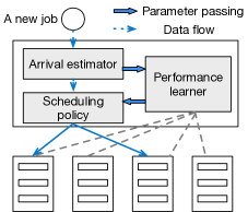
We present Rosella, a high-throughput and low-latency self-driving scheduler for heterogeneous systems. Rosella continuously adjusts its policy as the workers’ compute power fluctuates in a self-driving way. Rosella learns the workers’ processing power and acts on the learned parameters simultaneously. Specifically, Rosella possesses the following salient features (see also Fig. 1):

1. Efficiently learning the parameters. Rosella efficiently estimates the processing power of each worker. Rosella’s learning-time scales inverse-proportional to the load ratio, and logarithmically to the number of servers. Both dependencies are essentially optimal, making the scheduler highly scalable. For example, when the number of servers doubles, learning time only increases by a constant unit of times.

2. Heterogeneity-aware schedulers. We unify two major scheduling techniques in our job-allocation algorithm. The first is the so-called proportional sampling strategy [gandhi2015halo]. When a new task arrives, the scheduler chooses a worker according to a multinomial distribution so that the probability that the $i$ -th worker is chosen is proportional to its compute-power, e.g., if the $i$ -th worker is five times faster than the $j$ -th worker, the $i$ -th worker is five times more likely to be chosen. The second is the power-of-two-choices [Mitzenmacher00thepower] (PoT) strategy. When a new task arrives, we execute the proportional sampling algorithm twice to obtain two candidate workers and assign the task to the worker with the shorter queue.

In summary, we make the following contributions:

$\bullet$ We analyze the root causes why prior scheduling algorithms fail to provide high-throughput and low latency in a heterogeneous cloud system.

$\bullet$ We propose an algorithm to schedule jobs to a cluster with different compute-power workers. Compared to prior work, our scheduling algorithm reduces the worst-case queue length from $O(\log n)$ to $O(\log\log n)$ .

$\bullet$ We implement our algorithm on top of Spark [spark] scheduler. Extensive experiments of real-life workloads on a 32-node AWS cluster demonstrate that Rosella significantly outperforms a state-of-the-art scheduler [ousterhout2013sparrow] by $65\%$ in response time, and also is robust against various workloads in the dynamic and heterogeneous cluster.

II Problem Setting

Refer to caption — Figure 1: The architecture of Rosella: it continuously learns backend workers’ performance and adjusts its scheduling policy.

We consider a distributed system that consists of $n$ workers. Jobs may contain one or more tasks. When a new job arrives, the scheduler can probe a certain number of workers and decide how the tasks should be assigned to the workers based on their queue length. $\lambda$ is total arrival rate. The compute power of the workers is heterogeneous. The processing/service rate for worker $i$ is $\mu_{i}$ . Let $\mu=\sum_{i\leq n}\mu_{i}$ be the system’s the total processing power, and $\alpha=\lambda/\mu$ be the system’s load ratio. Both $\mu_{i}$ and $\lambda$ can change over time to reflect volatility in the system. We aim to design a simple scheduling algorithm that simultaneously optimizes the following metrics:

1. Response time. When a job arrives, how much time does the system need to process the job?

2. Learning and recovery time. When a system experiences a shock (many $\mu_{i}$ s changed), the scheduler does not have accurate estimates of the service rates of the workers ( $\mu_{i}$ s). How much time does the system need to re-learn the $\mu_{i}$ s, and once learned, how much time does the system need to recover (e.g., handling the backlogs produced by the scheduler using inaccurate estimates of $\mu_{i}$ s)?

III Motivation

Learning and scheduling algorithms have been widely studied [smith1978new, Mitzenmacher00thepower, McDiarmid05, moseley2011scheduling, lin2013joint, xie2015power, ying2017power, 258866, 258870, humphries2021case, kaffes2019centralized], but none are directly applicable in our setting. Below, we review the commonly used scheduling algorithms and learning algorithms and explain why they are not applicable.

III-A Scheduling Algorithms

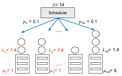
Uniform algorithm. When a new job arrives, the scheduler uniformly chooses a worker to serve it [Mitzenmacher2005]. When all $\mu_{i}$ s are uniform, the system consists of $n$ independent standard queues. At each time unit, each queue receives $\lambda/n$ tasks and can process $\mu/n$ tasks. All queues can process more tasks than they receive and thus all of them are stationary. The expected length of the largest queue is $O(\log n)$ . The uniform algorithm fails work when the service rates are different for different servers, i.e., by assigning the same amount of jobs to each server, the faster servers are underloaded and slower servers are overloaded.

Example 1.

Fig. 2a shows the example of uniform algorithm does not work. Assume there are 10 workers. The service rates for workers 1 to 9 are 1. The service rate for worker 10 is 6. The arrival rate is $14$ . The uniform algorithm assigns 10% of jobs to worker 1 (i.e., $\lambda_{1}=1.4$ ) but $\mu_{1}=1$ , implying that in the long run, worker 1 needs to process more tasks than its capacity.

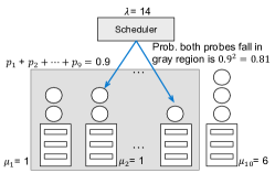
Power of two choices (PoT). When a new task arrives, the scheduler probes two random workers and assigns the new job to the worker with shorter queue. The PoT algorithm has improved worst-case queue length when the workers are homogeneous i.e., with high probability the largest queue length is $O(\log\log n)$ [Mitzenmacher00thepower]. However, the PoT algorithm suffers the same problem where slower workers are overloaded in the heterogeneous environment.

Example 2.

Fig. 2b shows the example of PoT does not work. Using the same configuration in Example 1, With probability $0.9\times 0.9=0.81$ , the scheduler selects 2 slow workers so one of them will process the job. On average there are $14\times 0.81=11.34$ jobs arriving at the slow workers, but the slow workers’ total processing power is only $9$ , implying that in the long run the slow workers need to process more jobs than their capacity.

Heterogeneity-aware load balancing. Recent attempts address the heterogeneity issue via assigning more jobs to more powerful workers [gandhi2015halo]. However, they impractically assume accurate knowledge of the servers’ processing powers and the processing powers do not change over time.

III-B Learning Algorithms

Explore-exploit paradigm. One reliable way to estimate $\mu_{i}$ is to compute the average processing time of the sufficient recent tasks. The explore-exploit paradigm arises because we do not want to assign many jobs to slow workers (i.e., exploit more powerful ones) and we also want to closely track the slower workers’ processing power so that we can use it when it becomes faster (explore the weaker ones).

The explore-exploit paradigm has been widely studied (e.g., multi-arm bandit problems [bubeck2012regret]), but the solutions mostly focus on the so-called regret bound. Regret analysis assumes that the regrets are memoryless, (i.e., a wrong decision is only penalized once). However, in our setting, a wrong decision may have a long-lasting effect (i.e., an adversarial impact on all subsequent load-balancing decisions).

Our learning objective. Instead of minimizing the regret, our learning and schedule algorithm simultaneously must 1. Efficiently learn the processing power. When the system is cold-started or has recently experienced a shock, the algorithm needs to efficiently (re)-learn the workers’ processing power; 2. Rapidly converge to the stationary distribution. When the algorithm re-learns the workers’ processing power, the system rapidly converges to the stationary distribution (i.e., efficiently handles the backlogs from using inaccurate/old processing power estimates); and 3. Be robust against estimation errors. The scheduler must work well in the presence of small estimation error.

IV System Design

This section explains Rosella’s architecture, and the operational details. Fig. 1 shows the architecture and the three main components: arrival estimator (Sec. IV-A), scheduling policy (Sec. IV-B) and performance learner (Sec. IV-C). When a job arrives, it goes to the arrival estimator, which estimates and updates the arrival rate $\lambda$ of the system. Next, the job goes to the scheduling policy, which uses the estimates of $\mu_{i}$ provided by the performance learner to choose the appropriate worker. The performance learning, which operates in the background, continuously maintains current estimates of each worker’s processing power. It takes the estimate $\lambda$ as input and determines how to communicate with the workers.

Technical challenges. 1. Power-of-two generalization. Recall that a classical PoT algorithm uniformly samples two workers, and uses the one with lighter loads to process the new job. Generalization of the PoT algorithm requires us to use non-uniform sampling (see Sec. IV-B for further discussions), and redefine the rule of choosing a worker because both of the two policies below are plausible (see e.g., [foss1998stability, foley2001join, bramson2010randomized, bramson2012asymptotic]):

1.

The join the shortest queue policy ( $\mathrm{SQ}$ ): assigns the incoming job to the queue with the shorter length.
2.

The join the least loaded queue policy ( $\mathrm{LL}$ ): assigns the incoming job to the queue with shorter waiting time.

Sec. IV-B discusses our design choice on these policies.

2. The explore-exploit paradigm and more jobs are better. Our performance learning component must balance the tradeoffs between estimating slow workers (that could potentially become fast) and assigning more jobs to fast workers. While this is a classical explore-exploit paradigm extensively studied in multi-arm bandit problems, one key difference is that in multi-arm bandit problems, a scheduler needs to passively perform the explore operations (e.g., only when a job arrives can the scheduler use it to explore) the workers’ performance; whereas our algorithm can actively explore servers’ performance by creating new jobs.

Optimizing the learning performance involves carefully controlling the number of jobs that need to be to be created for the purpose of exploration. Creating too few jobs will not accelerate the learning process, while creating too many jobs will slow down the whole system.

IV-A The arrival estimator

This component estimates $\lambda$ , using the mean interarrival time for the last $S$ jobs as the estimation of $1/\lambda$ . Here, $S$ is a hyperparameter. When $S$ is large, the estimate of $\lambda$ is more accurate, but the system reacts more slowly to the change of worker speeds. When $S$ is small, the estimate of $\lambda$ is less accurate, but the system reacts more rapidly to the environment changes.

IV-B The scheduling policy

The scheduling policy component (Fig. 3) has access to estimates $\hat{\mu}_{i}$ from the performance learning component and schedule the jobs. Our policy deviates from the classical PoT algorithms in two major ways.

1. Proportional sampling schedule (PSS). To circumvent heterogeneity of the workers, our approach probes faster workers with higher probability. Let $p_{i}=\hat{\mu}_{i}/(\sum_{i\leq n}\hat{\mu}_{i})$ . The proportional sampling procedure samples a worker from a multinomial distribution $(p_{1},p_{2},...,p_{n})$ . When the $\hat{\mu}_{i}$ ’s are accurate, workers behave like independent queues under proportional sampling with high probability that the maximum queue length is $O(\log n)$ .

2. Power-of-two-choices with $\mathrm{SQ}$ . We integrate PoT techniques to further reduce the maximum queue length, i.e., we use PSS to choose two workers and place the new job to the better one. We can use $\mathrm{SQ}$ or $\mathrm{LL}$ policy. Rosella uses $\mathrm{SQ}$ since it avoids using slower servers until too many jobs are waiting at the faster server:

Example 3.

A system consists of $n=\mu+1$ worker, where $\mu\gg 1$ is an integer. Worker 1’s processing rate is $\mu$ and the other servers’ processing rate is 1. The total processing rate is $2\mu$ , and the first server is substantially faster. The arrival rate of the jobs is $1.5\mu$ .

The probability that worker 1 is chosen as a candidate is $1-\left(\frac{1}{2}\right)^{2}=\frac{3}{4}$ . When worker 1 is chosen as a candidate, it will pick up the new job if it has less than $\mu-1$ jobs because the expected processing time for the other workers is at least $1$ (even assuming the other candidate’s queue is empty), whereas the expected processing time of worker 1 is $<1$ when it has less than $\mu-1$ jobs.

Assume that the system starts with empty queues at time $0$ . In the beginning, the arrival rate to worker 1 is $1.5\mu\times\frac{3}{4}=\frac{9}{8}$ while its processing rate is $\mu$ . Thus, the queue quickly builds up until its length hits $\mu-1$ . The queue will not shrink much afterward because as worker 1’s queue decreases, worker 1 will attempt to pick up more jobs. Thus, in the stationary state, the length of queue 1 is around $\mu-1$ , and the expected waiting time for a job at worker 1 is $(\mu-1+1)/\mu=1$ , which is as slow as the other slow servers.

In general, more jobs will be congested at the faster workers; all the workers could be as slow as the slowest server. In the $\mathrm{SQ}$ policy, however, slower workers will be utilized before faster servers become too full, alleviating the congestion problem.

{codebox}\Procname

$\proc{PPoT-Scheduling-policy}(s_{i})$ \li\Comment $s_{i}$ is the $i$ -th job. \liLet $p_{i}=\frac{\hat{\mu}_{i}}{\sum_{i\leq n}\hat{\mu}_{i}}$ \liLet $\vec{p}=(p_{1},\dots,p_{n})$ . \li $j_{1},j_{2}\leftarrow\mathrm{multinomial}(\vec{p})$ . \li\Commentlet $q_{i}$ be the length of queue $i$ . \li $j^{*}=\arg\min_{j\in\{j_{1},j_{2}\}}\{q_{i}\}$ . \li\Commentplace the job at the $j^{*}$ -th server.

Figure 3: Pseudocode for our proportional-sampling+PoT scheduling.

IV-C Performance learner

The performance learner, which operates in the background, continuously maintains current estimates of each worker’s processing power. It takes the estimate of $\lambda$ as input and uses it to determine how often to communicate with the workers. The performance learner actively generates new jobs and assigns them to the workers (see $\proc{Learner-Dispatcher}$ in Fig. 4). The jobs serve as benchmarks to estimate the workers’ processing powers.

Rosella generates the benchmark jobs according to a Poisson process with parameter $c_{0}(\bar{\mu}-\hat{\lambda})$ , where $\bar{\mu}$ is the minimum guaranteed service throughput, $\hat{\lambda}$ is the estimate of arrival rates, and $c_{0}$ is a small constant (say 0.1). Generating jobs at this frequency ensures that we optimally monitor all resources in the cluster while not jamming the system and slowing down the processing of other jobs. The benchmark jobs have low priorities, which will not be executed if other “real” jobs are waiting in the worker.

Choosing benchmark jobs. The benchmark jobs shall resemble recent workloads. For example, they can be replicates of the most recent queries at the frontend.

Learning. When worker $i$ completes computation of a job, it will communicate with the performance learner to update its estimate $\hat{\mu}_{i}$ (see $\proc{Learner-aggregate}$ in Fig. 4). The estimate is based on computing the average processing time of the last $L$ jobs, where $L=\Theta(\frac{\log(1/n)}{(1-\hat{\alpha})^{2}})$ , and $\hat{\alpha}=\hat{\lambda}/\bar{\mu}$ is the estimated load ratio. The historical window length depends on the load ratio $\alpha$ and total number of jobs $n$ for the following reasons: When $\alpha$ is small, there are sufficient residual compute resources so we can afford to have sloppy estimates. Therefore, the size of the historical window shrinks when $\alpha$ decreases. There is also a dependency on $\log 1/n$ because we need to use the standard Chernoff/union bound techniques to argue that all estimates are in reasonable quality (see Sec. LABEL:sec:analysis for the analysis).

When a worker is slow, it may take time to collect the statistics over its most recent $L$ tasks. Therefore, we set a waiting time cut-off, i.e., if we cannot estimate $\mu_{i}$ in $(1+\epsilon)L/\mu^{*}$ time (the variables in the Fig. 4), we set the estimate as 0, effectively treating the small worker as dead.

{codebox}\Procname

$\proc{Learner-Dispatcher}$ \li\CommentDispatches benchmark jobs to workers \liSample $t_{i}\sim\mathrm{Poisson}\left(0.1(\bar{\mu}-\hat{\lambda})\right)$ . \liAt time $t_{i}$ : $j\leftarrow\mathrm{Uniform}([n])$ . \liAssign a low priority job to worker $j$ .

{codebox}
\Procname

$\proc{Learner-aggregate}(\mbox{worker }i)$ \li\CommentCommunicate with performance learner \li $\hat{\alpha}\leftarrow\hat{\lambda}/\bar{\mu}$ , $\epsilon=\frac{3}{10}(1-\alpha)$ , $\mu^{*}=(1-\hat{\alpha})/10$ . \li $L\leftarrow\frac{c_{1}}{\epsilon^{2}}\log(1/n)$ for some constant $c_{1}$ . \liLet $\hat{q}_{i}$ be the average processing time \li for the most recent $L$ jobs \li\Ifcannot measure $\hat{q}_{i}$ in $(1+\epsilon)L/\mu^{*}$ time, $\hat{\mu}_{i}=0$ . \li\Commentthe workers too slow \li\Else $\hat{\mu}_{i}=(1-\epsilon)1/\hat{q}_{i}$ \End\liReport $\hat{\mu}_{i}$ to the performance learner

Figure 4: Pseudocode for the performance learner.