WASP-186 and WASP-187: two hot Jupiters discovered by SuperWASP and SOPHIE with additional observations by TESS

Abstract

We present the discovery of two new hot Jupiters identified from the WASP survey, WASP-186b and WASP-187b (TOI-1494.01 and TOI-1493.01). Their planetary nature was established from SOPHIE spectroscopic observations, and additional photometry was obtained from TESS. Stellar parameters for the host stars are derived from spectral line, IRFM, and isochrone placement analyses. These parameters are combined with the photometric and radial velocity data in an MCMC method to determine the planetary properties. WASP-186b is a massive Jupiter (4.22$\pm{0.18}\ M_{J}$, 1.11 $\pm{0.03}\ R_{J}$) orbiting a mid-F star on a 5.03 day eccentric (e=0.327$\pm{0.008}$) orbit. WASP-187b is a low density (0.80 $\pm{0.09}\ M_{J}$, 1.64 $\pm{0.05}R_{J}$) planet in a 5.15 day circular orbit around a slightly evolved early F-type star.

1 Introduction

While hot Jupiters are relatively rare, occurring for less than 1 star in 100 (Zhou et al., 2019), they are valuable because they are extreme examples of planetary-system formation. Because these planets have deep transits and short periods, they are well suited for discovery by ground-based surveys such as the Hungarian-made Automated Telescope Network (HATnet; Bakos et al., 2004), HATSouth (Bakos et al., 2013), the Qatar Exoplanet Survey (QES; Alsubai et al., 2013), the Kilodegree Extremely Little Telescope (KELT; Pepper et al., 2007), the Wide-Angle Search for Planets (WASP; Pollacco et al., 2006), and the Next-Generation Transit Survey (NGTS; Wheatley et al., 2018). As these small-aperture ground surveys are able to detect planets around bright stars, the resulting planet population is useful for follow-up studies of atmospheric composition and structure using occultation and transmission spectroscopy (e.g. Sing et al., 2015; Line et al., 2016).

In this study, we present the discovery of two new hot Jupiter planets: WASP-186b and WASP-187b (TOI-1494.01 and TOI-1493.01). Using Radial Velocity (RV) data from SOPHIE as well as photometry from WASP and TESS, we determine joint probability distributions for the system parameters. In section 2 we describe the observations of both stars with section 3 describing the method used to fit the planet transit and RV data. Finally, section 4 provides discussion of the new planets in the context of the known population of exoplanets.

2 Observations

Both WASP-186 and WASP-187 were originally flagged as candidates in the WASP survey data after an initial search of the data using the Box-Least-Squares (BLS) method (Kovács et al., 2002) using the implementation from Collier Cameron et al. (2006). The planetary nature of both candidates was established with follow-up RV data from the SOPHIE spectrograph (Perruchot et al., 2008; Bouchy et al., 2009b). Additionally, both of these planets were recently observed in photometry taken by the Transiting Exoplanet Survey Satellite (TESS; Ricker et al., 2015). A list of all of the observations can be found in Table 1, with further information found in the following sections.

Table 1: Summary of available photometric and radial velocity observations for WASP-186 and WASP-187.

Date	Source	No.obs
WASP-186b
2006 Aug - 2014 Jan	SuperWASP	81 014
2019 Oct - 2019 Nov	TESS	821
2016 Nov - 2017 Nov	SOPHIE HE	25
WASP-187b
2004 Jun - 2011 Nov	SuperWASP	15 278
2019 Oct - 2019 Nov	TESS	821
2014 Dec - 2016 Aug	SOPHIE HR	19
2016 Sep - 2017 Feb	SOPHIE HE	13

2.1 WASP Photometry

WASP-186 was observed by SuperWASP beginning in 2006 and ending in 2014 with a total of 81,014 30-second exposures. The star was originally flagged for further review in July 2016 after inspection of the lightcurve. WASP-187 was observed from 2004 until 2011 with a total of 15,278 observations. In 2014, the target was flagged for further observations.

The ORCA-TAMTFA transit-search run, which includes multi-season data on 480 fields in the region around the celestial equator that was observed by both SuperWASP and WASP-South, 716 fields from SuperWASP only and 553 from WASP-South only, is the largest and most homogeneous dataset available for WASP. As such, the photometry from this run was used as the basis for analysis by the machine learning method described in Schanche et al. (2019). This work combined the results of a Random Forest Classifier and Convolutional Neural Network to find and rank transit candidates. The field in which WASP-186 was identified as a candidate is not part of this run; however, WASP-187 was included and was identified as a good planetary candidate.

2.2 SOPHIE spectroscopy

Both WASP-186 and WASP-187 were observed with the SOPHIE spectrograph, first to establish the planetary nature of the SuperWASP transiting candidates, then to determine their masses and orbital eccentricities. SOPHIE is dedicated to high-precision RV measurements at the 1.93-m telescope of the Haute-Provence Observatory (Perruchot et al., 2008; Bouchy et al., 2009b)) and is widely used for SuperWASP follow-up (e.g. Collier Cameron et al. (2007a); Hébrard et al. (2013); Schanche et al. (2019)).

WASP-187 was observed between Dec. 2014 and Aug. 2016 in High-Resolution (HR) mode with a resolving power $R=76\,000$ and fast readout mode. Further data were taken between Sept. 2016 and Feb. 2017 in High-Efficiency (HE) mode with a resolving power $R=40\,000$ and slow readout mode. HR and HE observations could present a systematic radial velocity shift, so they are considered below as independent datasets. WASP-186 was observed between Nov. 2016 and Nov. 2017, only in HE mode and slow readout mode. Two low signal-to-noise observations of WASP-186 were not used.

The spectra were extracted using the SOPHIE pipeline (Bouchy et al., 2009b) and the radial velocities were measured from the weighted cross-correlation with a numerical mask (Baranne et al., 1996; Pepe et al., 2002). They were corrected for the CCD charge transfer inefficiency (Bouchy et al., 2009a) and their error bars were computed from the cross-correlation function (CCF) using the method presented by Boisse et al. (2010). Following the method described e.g. in Pollacco et al. (2008) and Hébrard et al. (2008), we estimated and corrected for moonlight contamination by using the second SOPHIE fiber aperture which is targeted on the sky while the first aperture points toward the star. The monitoring of constant stars revealed no significant instrumental drifts at the epochs of the observations.

The radial velocities are reported in Table 2. They have larger uncertainties than is typical for SOPHIE due to the rotational line broadening. The resulting CCFs have full width at half maximum of 22 and 21 km/s for WASP-186 and WASP-187, respectively. Still, they show significant variations in phase with the SuperWASP transit ephemeris, with semi-amplitudes corresponding to companions in the planetary-mass regime.

Radial velocities measured using different stellar masks (F0, G2, K0, or K5) produce variations with similar amplitudes, so it is unlikely that these variations are produced by blend scenarios composed of stars of different spectral types. We also checked for signals in the line asymmetry due to blending or magnetic activity using the line bisector measured using the approach of Boisse et al. (2010). They are plotted in Fig. 1 and show no variations correlated with RVs (Pearson correlation coefficients of -0.29 and -0.03 for WASP-186 and 187, respectively). We can thus conclude the the RV variations are not due to spectral-line profile changes attributable to blends or stellar activity, but rather to Doppler shifts due to planetary-mass companions.

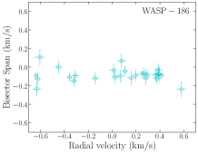
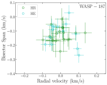
Figure 1: Bisector spans as a function of radial velocities for WASP-186 (left) and WASP-187 (right). The radial velocities shown in x-axis are obtained after subtracting the average radial velocity. For WASP-187, green and blue circles correspond to the data taken in HE and HR modes, respectively. Note that the 55.4-m/s fitted shift between HR and HE RVs of WASP-187 is corrected here.

Table 2: SOPHIE measurements of the planet-host stars

BJDUTC	RV	$\pm$$1\,\sigma$	bisect.∗	exp.	SNR†
-2 450 000	(km/s)	(km/s)	(km/s)	(sec)
WASP-186 = TOI-1494 (HE mode)
7719.3870	-5.655	0.031	-0.071	257	25.3
7721.5162	-6.064	0.033	-0.120	420	26.3
7744.3659	-5.628	0.031	-0.082	149	25.9
7745.3613	-6.244	0.031	-0.150	165	25.7
7746.3741	-6.230	0.031	-0.092	208	26.2
7778.2913	-5.529	0.045	-0.076	900	19.6
7791.3104	-6.528	0.043	0.107	1200	23.2
7792.2705	-5.843	0.039	0.067	272	25.3
7977.6056	-6.280	0.025	-0.109	900	36.0
7988.6111	-5.669	0.015	-0.070	900	55.9
7989.6207	-5.511	0.013	-0.092	900	61.1
7992.5287	-6.371	0.032	-0.001	229	26.0
8003.5848	-5.762	0.040	-0.115	412	25.1
8008.6203	-5.724	0.033	-0.086	282	25.3
8036.4419	-5.855	0.035	-0.098	382	26.4
8037.5082	-6.559	0.014	-0.090	900	59.2
8038.4968	-5.910	0.035	-0.034	321	26.6
8039.5341	-5.548	0.031	-0.122	196	26.1
8040.4692	-5.533	0.032	-0.074	263	26.2
8041.4421	-5.816	0.029	-0.044	188	29.0
8052.4838	-6.547	0.031	-0.127	147	25.9
8053.4492	-5.898	0.032	-0.108	342	25.6
8054.4030	-5.556	0.035	-0.086	514	25.2
8057.4893	-6.554	0.038	-0.237	441	25.5
8085.4759	-5.537	0.035	-0.030	245	26.7
WASP-187 = TOI-1493 (HR mode)
7020.3536	-20.287	0.029	-0.144	1400	37.5
7047.2607	-20.262	0.057	-0.072	1400	16.9
7247.6246	-20.236	0.039	-0.100	508	26.0
7275.6507	-20.188	0.038	-0.121	407	25.7
7303.4805	-20.284	0.020	0.028	1400	45.1
7306.5457	-20.222	0.039	-0.271	708	25.1
7309.5569	-20.217	0.041	-0.061	994	25.0
7331.5082	-20.194	0.023	-0.194	684	39.7
7332.5412	-20.151	0.026	-0.225	628	37.2
7333.5243	-20.258	0.030	-0.051	1400	33.9
7334.4887	-20.241	0.022	-0.195	655	39.4
7335.3682	-20.281	0.036	-0.090	300	25.4
7401.2935	-20.295	0.038	-0.070	676	25.0
7623.5982	-20.224	0.037	-0.053	384	25.1
7624.6495	-20.217	0.045	-0.171	445	22.1
7625.6060	-20.098	0.036	-0.243	499	24.9
7627.6290	-20.228	0.038	-0.157	446	25.3
7628.6165	-20.333	0.038	-0.150	520	25.1
7629.5948	-20.275	0.041	-0.077	1619	23.1
WASP-187 = TOI-1493 (HE mode)
7658.6570	-20.348	0.026	-0.111	638	32.6
7659.5249	-20.327	0.015	-0.164	916	50.8
7660.4893	-20.276	0.024	-0.113	319	32.0
7661.5282	-20.205	0.024	-0.117	281	32.1
7681.5194	-20.243	0.027	-0.104	445	31.8
7682.5562	-20.188	0.027	-0.168	258	32.6
7720.4122	-20.338	0.024	-0.137	277	32.3
7721.5065	-20.375	0.025	-0.076	545	33.0
7744.3363	-20.198	0.023	-0.158	138	32.2
7745.3565	-20.260	0.023	-0.113	171	32.0
7746.3691	-20.339	0.023	-0.016	181	33.1
7778.2806	-20.335	0.023	-0.163	485	33.0
7792.2768	-20.305	0.029	-0.166	263	30.3
$\ast$: bisector spans; error bars are twice those of the RVs.
†: signal-to-noise ratio per pixel at 550 nm.

2.3 TESS photometry

In October and November 2019, both candidates were observed in Sector 17 of the TESS mission and given the designations as TESS Objects of Interest (TOI)-1494.01 and TOI-1493.01 with four transits observed for each target. However, a momentum dump at the beginning of the observation run coincided with the first transit of WASP-186 leading the affected transit to appear deeper. We therefore remove the first transit from further analysis. Although the event did not disrupt a transit for WASP-187, we remove the data for this time frame to remove any impact on the out-of-transit measurement. Additionally, the data surrounding spacecraft perigee was removed for both lightcurves.x The Full Frame Images (FFIs) have a cadence of 30 minutes, with each image comprising a stack of 2 second exposures over that time frame. The data were downloaded and the lightcurves were extracted and long term trends were removed using the functions provided in the lightkurve package (Lightkurve Collaboration et al., 2018). We checked both stars for centroid shifts, but no shifts corresponding to the transits were detected, supporting the conclusion that the transits occur on the target star.

3 Analysis

3.1 Spectral Characterization

For each star, the SOPHIE spectra not polluted by Moonlight were shifted to a common radial velocity and co-added. The spectral analyses were performed using the process outlined in Doyle et al. (2013), i.e. the stellar effective temperature ($T_{\rm eff}$) was found using the $H\alpha$ line; the stellar surface gravity (log $g$) was determined from the Na D and Mg b lines; the metallicity was estimated from the width of several Fe I lines; and the projected rotational velocity (v sin i) was determined by convolving the SOPHIE spectrum with the instrumental profile and then using spectrum synthesis to fit the Fe I lines, in agreement with results obtained from the the CCF using the calibration of Boisse et al. (2010). The results of this spectral analysis can be found in Table 3.

Table 3: Initial stellar parameters from the spectroscopic ($T_{\rm eff}$, log $g$, Fe/H, and $v\sin{i}$), isochrone placement, ($M_{\ast}$ and Age), and Gaia+IRFM ($\varpi$, $R_{\ast}$) analysis of WASP-186 and WASP-187.

Parameter	WASP-186	WASP-187
$T_{\rm eff}$ (K)	$6300\pm 100$	$6100\pm 100$
log $g$	$4.1\pm 0.2$	$3.8\pm 0.2$
Fe/H	$-0.08\pm 0.14$	$0.0\pm 0.11$
$v\sin{i}$ (${\rm km\,s}^{-1}$)	$15.6\pm 0.9$	$15.3\pm 1.0$
$M_{\ast}$	$1.21^{+0.07}_{-0.08}$	$1.53^{+0.07}_{-0.09}$
Age (Gyr)	$3.1^{+1.0}_{-0.8}$	$2.55^{+0.49}_{-0.25}$
Parallax $\varpi$ (mas)	3.563 $\pm{0.042}$	2.667 $\pm{0.048}$
$R_{\ast}$ ($R_{\odot}$)	1.46 $\pm{0.02}$	2.87 $\pm{0.05}$

3.2 Gaia IRFM

The infrared flux method (IRFM), introduced by Blackwell & Shallis (1977), is a semi-direct way to measure stellar angular diameter and effective temperature. This method combines flux measurements at different wavelengths with stellar atmospheric models to determine the stellar properties. The IRFM method has been implemented by several groups, e.g. (Alonso et al., 1994; Ramírez & Meléndez, 2005; González Hernández & Bonifacio, 2009; Casagrande et al., 2010). Here we expand the method with the incorporation of data from Gaia.

The magnitudes and corresponding uncertainties for WASP-186 and WASP-187 in the Gaia G, $G_{\rm BP}$ and $G_{\rm RP}$ bandpasses (Riello et al., 2018) were retrieved from the second data release (DR2) archive (Gaia Collaboration et al., 2018), along with data taken in the J, H, and K filters from the 2MASS survey (Skrutskie et al., 2006) and in the W1 and W2 (3.4 and 4.6 $\mu$m) bandpasses from the WISE survey (Wright et al., 2010). This information is used together with the stellar synthetic spectra atlas of Castelli & Kurucz (2003) to find initial estimates of stellar effective temperature and angular diameter ($\theta$). The Gaia parallax measurement ($\varpi$) is then used to produce a radius measurement for the star.

3.3 Stellar Masses

Using stellar parameters derived from the spectral line fitting (shown in Table 3), stellar masses and ages for WASP-186 and WASP-187 were determined by the isochrone placement functionality of the mcmci tool (Bonfanti & Gillon, 2020). Following an MCMC approach, with five chains of 100 000 steps and a burn-in fraction of 20 per cent, stellar masses were calculated by interpolating over grids of stellar isochrones and evolutionary tracks to be $M_{\rm*}=1.21_{-0.08}^{+0.07}$ $M_{\odot}$ and $M_{\rm*}=1.53_{-0.09}^{+0.07}$ $M_{\odot}$ for WASP-186 and WASP-187, respectively. The corresponding stellar ages were found to be $3.1_{-0.8}^{+1.0}$ and $2.55_{-0.25}^{+0.49}$ Gyr. This places WASP-187 near the main-sequence turn-off on evolutionary tracks for the most probable range of masses.

3.4 Planetary Parameters

The MCMC approach is commonly used in exoplanet model fitting as it is efficiently able to fit a model to the data while at the same time providing a posterior probability distribution of each fitted parameter. The implementation used here is modeled on Collier Cameron et al. (2007b). The code aims to fit the stellar parameters along with the transit and RV data simultaneously.

The jump parameters used to describe the data are chosen to be independent of each other, therefore the fit of the data to the model relies on the transition of the MCMC jump parameters to the physical variables (For a full description of the transition from these jump parameters to physical variables, see Appendix A). The jump parameters used here are: the transit epoch ($T_{c}$), period ($P$), impact parameter ($b$), transit width ($w$), transit depth ($(R_{P}/R_{S})^{2}$), received flux ($f$), parallax ($\varpi$), stellar radius ($R_{\ast}$), extinction ($E(B{-}V)$), log of the system error which accounts for zero-point uncertainties in the definitions of the flux-to-magnitude conversions for the different bandpasses in the IRFM calculation ($\log{\sigma_{\rm sys}}$), RV amplitude ($K$), RV offset ($\gamma$), and RV jitter ($\sigma_{\rm jit}$). For WASP-187 the RV offset and jitter are treated separately for the High-Resolution and High-Efficiency modes. The eccentricity $e$ and argument of periastron $\omega$ are parameterized as $\sqrt{e}\cos{\omega}$ and $\sqrt{e}\sin{\omega}$; the fit to the orbit of WASP-187 was, however, found to be consistent with an eccentricity of 0. Therefore the final MCMC held these values constant. Finally, the transit depth of WASP-187 was underestimated when WASP data were included in the fit. There are no contaminating stars within 114 arcsec. The most likely explanation is a slight dilution of the signal from the detrending of the WASP data. To account for the dilution, we fit an additional positive, constant flux offset to the WASP fluxes for this star, thereby allowing the TESS data to dominate the depth determination while retaining the timing information provided by WASP.

Initial fits for the depth, width, impact parameter, period, and epoch for the photometric datasets were done using the Transit Model in the PyCHEOPS v0.6.0 Python package. The power-2 limb darkening coefficients (Maxted, 2018) are interpolated from tables for TESS and WASP separately for the initial fit, as well as at every step in the MCMC. The initial fit for the radial velocity parameters were obtained with the RadVel package.

Several additional pieces of prior information are incorporated into the model. Given $T_{\rm eff}$, $\log g$, and Fe/H, the stellar surface flux spectrum is computed and attenuated by a galactic extinction law characterised by $E(B{-}V)$. The resulting reddened spectrum is folded through the Gaia, 2MASS and WISE photon-weighted filter transmission curves and scaled by the zero-points and the squared angular radius to obtain synthetic apparent magnitudes. The residuals of the observed minus synthetic magnitudes in the eight bandpasses and their uncertainties contribute directly to the likelihood at each jump. There is also a prior imposed on the parallax from the measurement in Gaia DR2 ($3.562\pm 0.043$ and $2.664\pm 0.044$ mas for WASP-186 and WASP-187 respectively). $T_{\rm eff}$ and $\log g$ priors are imposed from the spectroscopic analysis described in section 3.1. Finally, the stellar mass prior was determined from the isochrone placement method described in section 3.3.

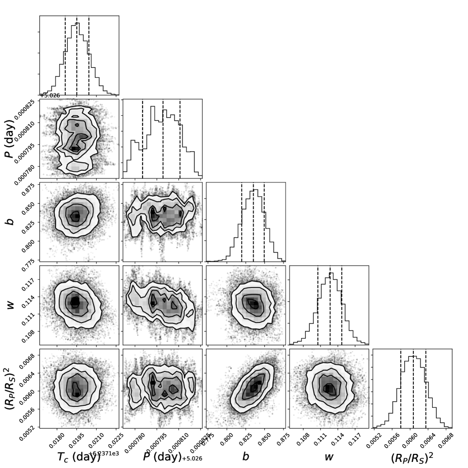
Figure 7: Cornerplot of the jump parameters describing the photometric data from the final MCMC run for WASP-186.

The MCMC went through 3 burn-in phases of 6 000, 2 000, and 2 000 steps, with updates of the jump lengths after each phase. The final MCMC was run for 50 000 steps. The final corner plots for the MCMC runs are shown in Figures 7 through 12 in the appendix. The resulting best-fit model for WASP-186b and WASP-187b are shown in Figures 2 and 3.

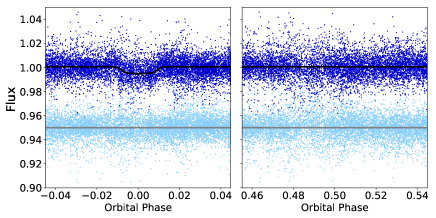
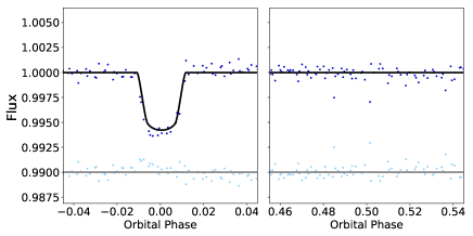
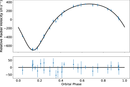
Figure 2: WASP (top), TESS (middle), and SOPHIE (bottom) data for WASP-186b phase folded on the best-fitting period. Residuals to the fit are shown below the data.

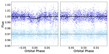
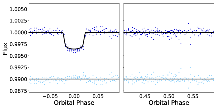
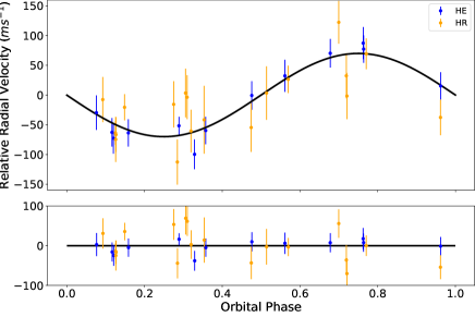
Figure 3: WASP (top), TESS (middle), and SOPHIE (bottom) data for WASP-187b phase folded on the best-fitting period. Residuals to the fit are shown below the data.

Table 4: System parameters for WASP-186 and WASP-187

Parameters	Symbol (Unit)	WASP-186	WASP-187
Stellar Parameters
WASP ID		1SWASP J011558.85+213700.9	1SWASP J010953.96+254054.0
TESS ID		TOI-1494.01/TIC-411608801	TOI-1493.01/TIC-15692883
Gaia ID		2790691147020786816	306410392895767680
Right Ascension	RA (hh:mm:ss)	01:15:58.85	01:09:53.96
Declination	Dec (dd:mm:ss)	+21:37:00.9	+25:40:54.0
Visual Magnitude	Vmag (mag)	10.82	10.30
TESS Magnitude	Tmag (mag)	10.30	9.71
Gaia Magnitude	Gmag (mag)	10.65	10.13
Stellar Mass	$M_{\ast}$ ($M_{\odot}$)	$1.22^{+0.07}_{-0.08}$	$1.54\pm 0.09$
Stellar Radius	$R_{\ast}$ ($R_{\odot}$)	$1.47\pm 0.02$	$2.83\pm 0.05$
Effective Temperature	$T_{\rm eff}$ (K)	$6361^{+105}_{-82}$	$6150^{+92}_{-85}$
Parallax	$\varpi$ (mas)	$3.571^{+0.044}_{-0.042}$	$2.663^{+0.046}_{-0.043}$
Stellar Density	$\rho_{s}$ ($\rho_{\odot}$)	$0.387^{+0.028}_{-0.027}$	$0.068\pm 0.005$
Surface Gravity	log $g$  (cgs)	$4.193^{+0.028}_{-0.029}$	$3.722\pm 0.029$
Received Flux	f*1e-9 (cgs)	$1.266^{+0.007}_{-0.006}$	$2.055\pm 0.008$
Extinction	$E(B{-}V)$ (mag)	$0.03\pm 0.02$	$0.09\pm 0.02$
Planet Parameters
Period	P (d)	$5.026799^{+.000012}_{-.000014}$	$5.147878^{+.000005}_{-.000009}$
Transit Epoch	Tc-2450000	$6237.1195\pm 0.0009$	$5197.3529^{+0.002}_{-0.0022}$
Transit Width	$w$ (hr)	$2.704^{+0.048}_{-0.051}$	$5.82^{+0.095}_{-0.091}$
Transit Depth	$(R_{P}/R_{S})^{2}$	$0.0061\pm 0.0003$	$0.0035\pm 0.0002$
Planet Mass	$M_{p}\ (M_{Jup})$	$4.22\pm 0.18$	$0.8\pm 0.09$
Planet Radius	$R_{p}\ (R_{Jup})$	$1.11\pm 0.03$	$1.64\pm 0.05$
Semi-major Axis	a (au)	$0.06^{+0.0012}_{-0.0013}$	$0.0653\pm 0.0013$
Impact Parameter	$b$	$0.84^{+0.01}_{-0.02}$	$0.76\pm 0.02$
Orbital Eccentricity	$e$	$0.33\pm 0.01$	0 (Fixed)
Argument of Periastron	$\omega$	$3.02^{+0.05}_{-0.06}$	0 (Fixed)
Planet Density	$\rho_{p}\ (\rho_{Jup})$	$2.881^{+0.3}_{-0.279}$	$0.169^{+0.026}_{-0.023}$
Surface Gravity	log $g$ (cgs)	$3.93\pm 0.03$	$2.87^{+0.05}_{-0.06}$
RV Semi-amplitude	K ($m\ s^{-1}$)	$530.29^{+8.43}_{-8.59}$	$70.0^{+6.84}_{-7.75}$
Zero-point Uncertainty	$\log{\sigma_{\rm sys}}$	$-2.19^{+0.41}_{-0.34}$	$-2.16^{+0.32}_{-0.25}$
RV offset	$\gamma$ ($m\ s^{-1}$)	$-5866.2^{+5.7}_{-5.6}$	$-20275.3^{+6.9}_{-6.8}$ (HE), $-20220.4^{+9.2}_{-9.3}$ (HR)
RV Jitter	$\sigma_{\rm jit}$ ($m\ s^{-1}$	$0.8^{+7.1}_{-7.3}$	$3.6^{+4.8}_{-2.8}$ (HE), $17.0^{+12.7}_{-8.7}$ (HR)

4 Discussion and Conclusions

The full set of parameters derived for WASP-186b and WASP-187b can be found in Table 4. Note that the values reported for $T_{\rm eff}$, stellar log $g$, $\varpi$, $M_{\ast}$ and $R_{\ast}$ were determined by the MCMC analysis and differ slightly from the prior values shown in Table 3.

WASP-186 is a mid-F type star with an effective temperature of $6361^{+105}_{-82}\,$K, agreeing with the spectral determination within errors. The parallax estimate corresponds to a distance of 280.71${}^{+13.05}_{-11.96}$ pc (Bailer-Jones et al., 2018). The star is rotating with a $v\sin{i}$ of $15.6\pm{0.9}\,{\rm km\,s}^{-1}$. As can be seen in Figure 4, the planet has a radius typical for a hot Jupiter ($1.11\pm{0.03}\,R_{\rm Jup}$), but is quite massive at $4.22\pm{0.18}\,M_{\rm Jup}$. WASP-186b therefore fits among the most massive and dense hot Jupiters known. WASP-186b is also notable as the orbit has an eccentricity of 0.33 $\pm{0.01}$, pointing to late-time high-eccentricity migration, rather than disc migration (Rasio & Ford, 1996; Ford & Rasio, 2008). Using equation 1 of Dobbs-Dixon et al. (2004) and an estimate for $Q^{\prime}_{p}$ of 10⁶ in line with the estimation from Yoder & Peale (1981), the time scale of eccentricity damping via tidal disturbance is on the order of 15.7 Gyr, well above the estimated age of 3.1${}^{+1.0}_{-0.8}$ Gyr. WASP-186b therefore joins the small group of massive and eccentric planets, including WASP-150b Cooke et al. (2020), WASP-162b (Hellier et al., 2019), HATS-41b (Bento et al., 2018), XO-3b (Johns-Krull et al., 2008), and HAT-P-2b (Bakos et al., 2007). Finally, the planet has an equilibrium temperature ($T_{eq}$) of $1348^{+23}_{-22}$ K, assuming zero albedo and isotropic blackbody re-radiation.

The host star for WASP-187b has begun to evolve away from the main sequence (see Fig. 5), indicated by the stellar effective temperature of $6150^{+92}_{-85}\,$K, mass of $1.54\pm{0.09}\,M_{\odot}$, and radius of $2.83\pm{0.05}\,R_{\odot}$. The star is 375.52$\pm{.45}$ pc away (Bailer-Jones et al., 2018) and has a projected rotation is similar to that of WASP-186 at 15.3 $\pm{1.0}\,{\rm km\,s}^{-1}$, indicating the rotation has slowed since leaving the main sequence (Wolff & Simon, 1997). WASP-187b is hotter ($T_{eq}=1726^{+31}_{-29}$) and significantly less dense than WASP-186b with a mass of $0.80\pm{0.09}\,M_{\rm Jup}$ and a radius of $1.64\pm{0.05}\,R_{\rm Jup}$, suggesting that this planet could be undergoing re-inflation (Hartman et al., 2016). Both planets have a period of around 5 days, but their radii lie near the low and high radius boundaries for known hot Jupiters of that period (see Fig. 6).

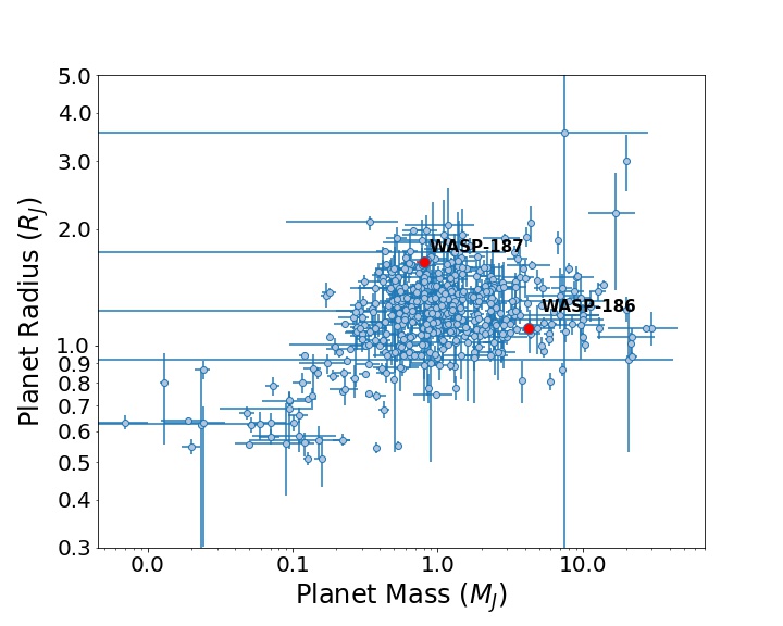
Figure 4: Planet mass versus planet radius for all Jupiter-sized planets ($R_{P}>0.5R_{J}$) with mass and radius measurements. Data for this and subsequent plots was obtained from the NASA Exoplanet Archive http://exoplanetarchive.ipac.caltech.edu.

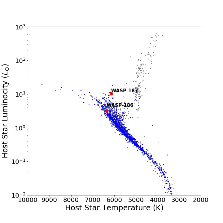
Figure 5: H-R diagram showing temperature versus stellar luminosity for all stars known to host exoplanets. Stars hosting planets with periods less than 10 days are shown in blue, while stars hosting planets with longer periods are in gray. Note that WASP-187 lies to the right of the main sequence, indicating that the star has entered the post-main sequence phase of its life.

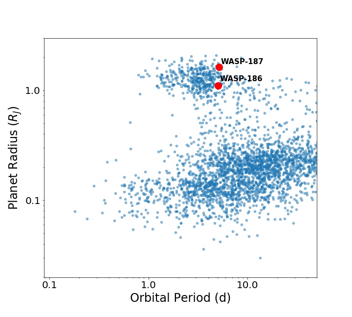
Figure 6: Orbital period versus planet radius for all known exoplanets with a period less than 50 days.

Data Availability

The data used in this publication can be accessed at https://doi.org/10.17630/c311756f-557e-4955-b50e-980633ded8f9

Appendix A State to Physical Variables

In order to convert the MCMC jump parameters ($P$, $w$, $d$, $b$, $\sqrt{e}\cos{\omega}$, $\sqrt{e}\sin{\omega}$, $f$, $\varpi$, $R_{\ast}$, $E(B{-}V)$, and $\log(\sigma_{\rm sys})$) to their physical meaning for the system, the following equations were used:

The eccentricity $e$ and argument of periastron $\omega$ are found using:

$$e=(\sqrt{e}\cos{\omega})^{2}+(\sqrt{e}\sin{\omega})^{2}$$ (1)

and

$$\omega=\tan^{-1}(\sqrt{e}\sin{\omega},\sqrt{e}\cos{\omega})$$ (2)

The transit duration (in days) that would be expected if the impact parameter were 0 is given by

$$w_{0}=\dfrac{w(1+k)}{\sqrt{(1+k)^{2}-b^{2}}}$$ (3)

where $w$ is a proxy for the transit width and $k$ is the ratio of the planetary to stellar radii, $R_{p}/R_{\ast}$. The ratio of the stellar radius to the semi-major axis is then given by

$$\dfrac{R_{\ast}}{a}=\dfrac{\pi\ w_{0}\ (1+e\sin{\omega})}{(1+k)P\sqrt{(1-e^{2})}}$$ (4)

where P is the orbital period in days. As described by Winn (2009), $\cos{i}$ and $\sin{i}$ are then calculated as

$$\cos{i}=b\dfrac{R_{\ast}}{a}\dfrac{1+e\sin{\omega}}{(1-e^{2})}\\ \sin{i}=\sqrt{1-\cos{i}^{2}}$$ (5)

The next step is to get the angular radius of the star. First the radius and parallax of the star are used to get the angular radius ($\theta\equiv\dfrac{R_{\ast}}{d}$):

$$\theta=\dfrac{R_{\ast}\ (\varpi+0.082)}{1000\star 180\star 3600}$$ (6)

where $\varpi$ is the parallax in milli-arcseconds, and the correction of Stassun & Torres (2018) is applied to the parallax.

The orbital separation can then be found by:

$$\dfrac{a}{a_{\oplus}}=\dfrac{\theta}{\varpi}\dfrac{a}{R_{\ast}}$$ (7)

with $a_{\oplus}$ being one astronomical unit and $\varpi$ expressed in radians.

The mass of the star can then be calculated using Kelper’s third law and appropriate unit conversions:

$$\dfrac{M_{\ast}}{M_{\odot}}=\left(\dfrac{a}{a_{\oplus}}\right)^{3}\left(\dfrac{P}{1{\rm year}}\right)^{-2}$$ (8)

The angular radius is also utilized to find the stellar surface flux $F$:

$$F=f/\theta^{2}.$$ (9)

The stellar surface flux is corrected for extinction iteratively:

$$F_{\rm ext}=F\ 10^{0.4\ E(B{-}V)\ R_{\rm bol}}.$$ (10)

$R_{\rm bol}$ used here is the bolomentric extinction to reddening ratio, determined by optimizing the fit to stellar radii in the asteroseismic samples provided in Silva Aguirre et al. (2015):

$$R_{\rm bol}=2.31+0.000509(T_{\rm eff}-5894)$$ (11)

The flux is then used to find the effective temperature $T_{\rm eff}$. In this way, the $T_{\rm eff}$ and $E(B{-}V)$ values are decoupled from the stellar radius.

With the mass and radius of the star now known, we can calculate $\log g$.

Finally, the power-2 limb darkening parameters are interpolated from a grid specific to each instrument using the $\log g$ and $T_{\rm eff}$ calculated.

The final physical variables therefore are $\sin{i}$, $\dfrac{R_{\ast}}{a}$, k, $T_{\rm eff}$, $\log g$, $\theta$, $M_{\ast}$ $\sigma_{\rm sys}$, $e$, and $\omega$.

Appendix B MCMC Results

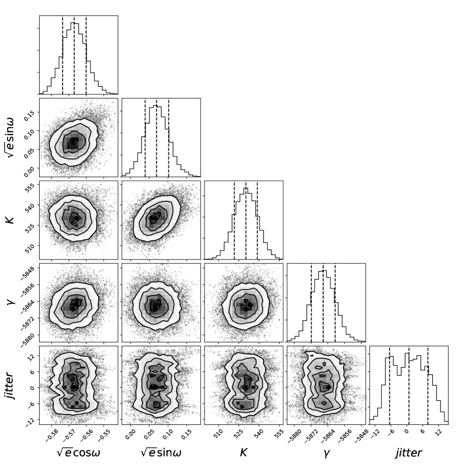
Figure 8: Cornerplot of the jump parameters describing the Radial Velocity data from the final MCMC run for WASP-186.

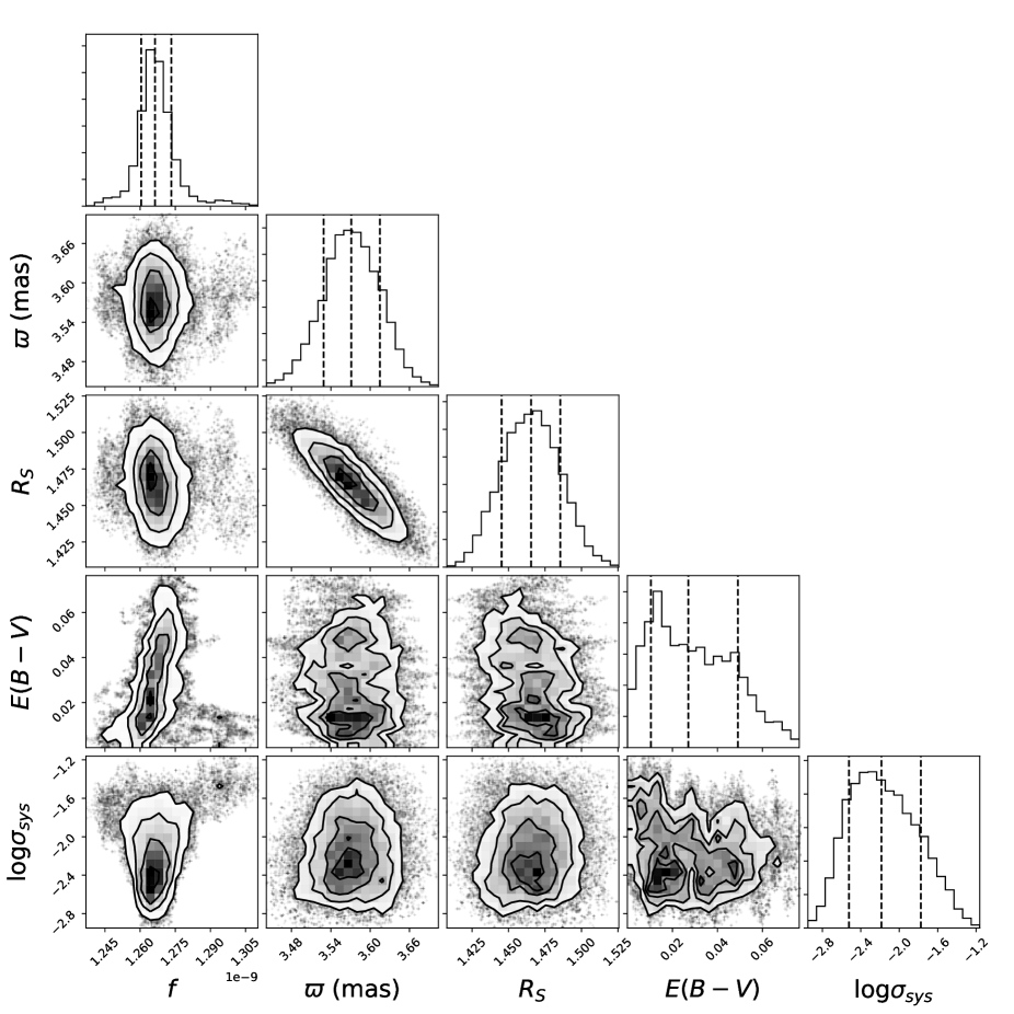
Figure 9: Cornerplot of the jump parameters describing the stellar features from the final MCMC run for WASP-186.

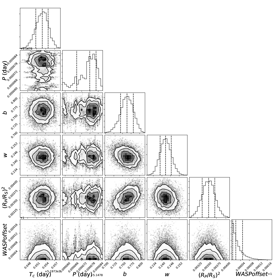
Figure 10: Same as Figure 7 but for WASP-187.

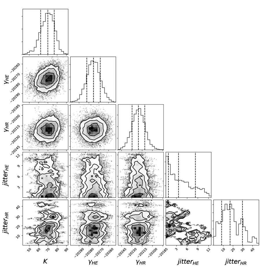
Figure 11: Same as Figure 8 but for WASP-187.

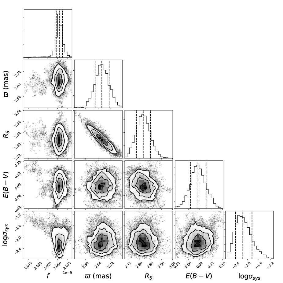
Figure 12: Same as Figure 9 but for WASP-187.

References

- Alonso et al. (1994) Alonso A., Arribas S., Martinez-Roger C., 1994, A&A, 282, 684
- Alsubai et al. (2013) Alsubai K. A., et al., 2013, Acta Astron., 63, 465
- Bailer-Jones et al. (2018) Bailer-Jones C. A. L., Rybizki J., Fouesneau M., Mantelet G., Andrae R., 2018, AJ, 156, 58
- Bakos et al. (2004) Bakos G., Noyes R. W., Kovács G., Stanek K. Z., Sasselov D. D., Domsa I., 2004, PASP, 116, 266
- Bakos et al. (2007) Bakos G. Á., et al., 2007, ApJ, 670, 826
- Bakos et al. (2013) Bakos G. Á., et al., 2013, PASP, 125, 154
- Baranne et al. (1996) Baranne A., et al., 1996, A&AS, 119, 373
- Bento et al. (2018) Bento J., et al., 2018, MNRAS, 477, 3406
- Blackwell & Shallis (1977) Blackwell D. E., Shallis M. J., 1977, MNRAS, 180, 177
- Boisse et al. (2010) Boisse I., et al., 2010, A&A, 523, A88
- Bonfanti & Gillon (2020) Bonfanti A., Gillon M., 2020, A&A, 635, A6
- Bouchy et al. (2009a) Bouchy F., Isambert J., Lovis C., Boisse I., Figueira P., Hébrard G., Pepe F., 2009a, in Kern P., ed., EAS Publications Series Vol. 37, EAS Publications Series. pp 247–253, doi:10.1051/eas/0937031
- Bouchy et al. (2009b) Bouchy F., et al., 2009b, A&A, 505, 853
- Casagrande et al. (2010) Casagrande L., Ramírez I., Meléndez J., Bessell M., Asplund M., 2010, A&A, 512, A54
- Castelli & Kurucz (2003) Castelli F., Kurucz R. L., 2003, in Piskunov N., Weiss W. W., Gray D. F., eds, IAU Symposium Vol. 210, Modelling of Stellar Atmospheres. p. A20 (arXiv:astro-ph/0405087)
- Collier Cameron et al. (2006) Collier Cameron A., et al., 2006, MNRAS, 373, 799
- Collier Cameron et al. (2007a) Collier Cameron A., et al., 2007a, MNRAS, 375, 951
- Collier Cameron et al. (2007b) Collier Cameron A., et al., 2007b, MNRAS, 380, 1230
- Cooke et al. (2020) Cooke B. F., et al., 2020, AJ, 159, 255
- Dobbs-Dixon et al. (2004) Dobbs-Dixon I., Lin D. N. C., Mardling R. A., 2004, ApJ, 610, 464
- Doyle et al. (2013) Doyle A. P., et al., 2013, MNRAS, 428, 3164
- Ford & Rasio (2008) Ford E. B., Rasio F. A., 2008, ApJ, 686, 621
- Gaia Collaboration et al. (2018) Gaia Collaboration et al., 2018, A&A, 616, A1
- González Hernández & Bonifacio (2009) González Hernández J. I., Bonifacio P., 2009, A&A, 497, 497
- Hartman et al. (2016) Hartman J. D., et al., 2016, AJ, 152, 182
- Hébrard et al. (2008) Hébrard G., et al., 2008, A&A, 488, 763
- Hébrard et al. (2013) Hébrard G., et al., 2013, A&A, 549, A134
- Hellier et al. (2019) Hellier C., et al., 2019, MNRAS, 482, 1379
- Johns-Krull et al. (2008) Johns-Krull C. M., et al., 2008, ApJ, 677, 657
- Kovács et al. (2002) Kovács G., Zucker S., Mazeh T., 2002, A&A, 391, 369
- Lightkurve Collaboration et al. (2018) Lightkurve Collaboration et al., 2018, Lightkurve: Kepler and TESS time series analysis in Python, Astrophysics Source Code Library (ascl:1812.013)
- Line et al. (2016) Line M. R., et al., 2016, AJ, 152, 203
- Maxted (2018) Maxted P. F. L., 2018, A&A, 616, A39
- Pepe et al. (2002) Pepe F., Mayor M., Galland F., Naef D., Queloz D., Santos N. C., Udry S., Burnet M., 2002, A&A, 388, 632
- Pepper et al. (2007) Pepper J., et al., 2007, PASP, 119, 923
- Perruchot et al. (2008) Perruchot S., et al., 2008, The SOPHIE spectrograph: design and technical key-points for high throughput and high stability. p. 70140J, doi:10.1117/12.787379
- Pollacco et al. (2006) Pollacco D. L., et al., 2006, PASP, 118, 1407
- Pollacco et al. (2008) Pollacco D., et al., 2008, MNRAS, 385, 1576
- Ramírez & Meléndez (2005) Ramírez I., Meléndez J., 2005, ApJ, 626, 446
- Rasio & Ford (1996) Rasio F. A., Ford E. B., 1996, Science, 274, 954
- Ricker et al. (2015) Ricker G. R., et al., 2015, Journal of Astronomical Telescopes, Instruments, and Systems, 1, 014003
- Riello et al. (2018) Riello M., et al., 2018, A&A, 616, A3
- Schanche et al. (2019) Schanche N., et al., 2019, MNRAS, 483, 5534
- Silva Aguirre et al. (2015) Silva Aguirre V., et al., 2015, MNRAS, 452, 2127
- Sing et al. (2015) Sing D. K., et al., 2015, MNRAS, 446, 2428
- Skrutskie et al. (2006) Skrutskie M. F., et al., 2006, AJ, 131, 1163
- Stassun & Torres (2018) Stassun K. G., Torres G., 2018, ApJ, 862, 61
- Wheatley et al. (2018) Wheatley P. J., et al., 2018, MNRAS, 475, 4476
- Winn (2009) Winn J. N., 2009, in Pont F., Sasselov D., Holman M. J., eds, IAU Symposium Vol. 253, Transiting Planets. pp 99–109 (arXiv:0807.4929), doi:10.1017/S174392130802629X
- Wolff & Simon (1997) Wolff S., Simon T., 1997, PASP, 109, 759
- Wright et al. (2010) Wright E. L., et al., 2010, AJ, 140, 1868
- Yoder & Peale (1981) Yoder C. F., Peale S. J., 1981, Icarus, 47, 1
- Zhou et al. (2019) Zhou G., et al., 2019, AJ, 158, 141