The public debt multiplier

Abstract

We study the effects on economic activity of a pure temporary change in government debt and the relationship between the debt multiplier and the level of debt in an overlapping generations framework. The debt multiplier is positive but quite small during normal times while it is much larger during crises. Moreover, it increases with the steady state level of debt. Hence, the call for fiscal consolidation during recessions seems ill-advised. Finally, a rise in the steady state debt-to-GDP level increases the steady state real interest rate providing more room for manoeuvre to monetary policy to fight deflationary shocks.

Keywords: Fiscal Policy, Public Debt, Multiplier, Overlapping Generations.

JEL classification: E52, E62, H63.

1 Introduction

In face of the Great Recession and the unprecedented fall in output, private consumption and investment spending, all advanced economies responded with a range of fiscal and monetary policy measures: increases in government spending, tax cuts, and various type of “unconventional”monetary policy measures, given that monetary policy was unable to lower further the nominal interest rate already close or at the zero lower bound.

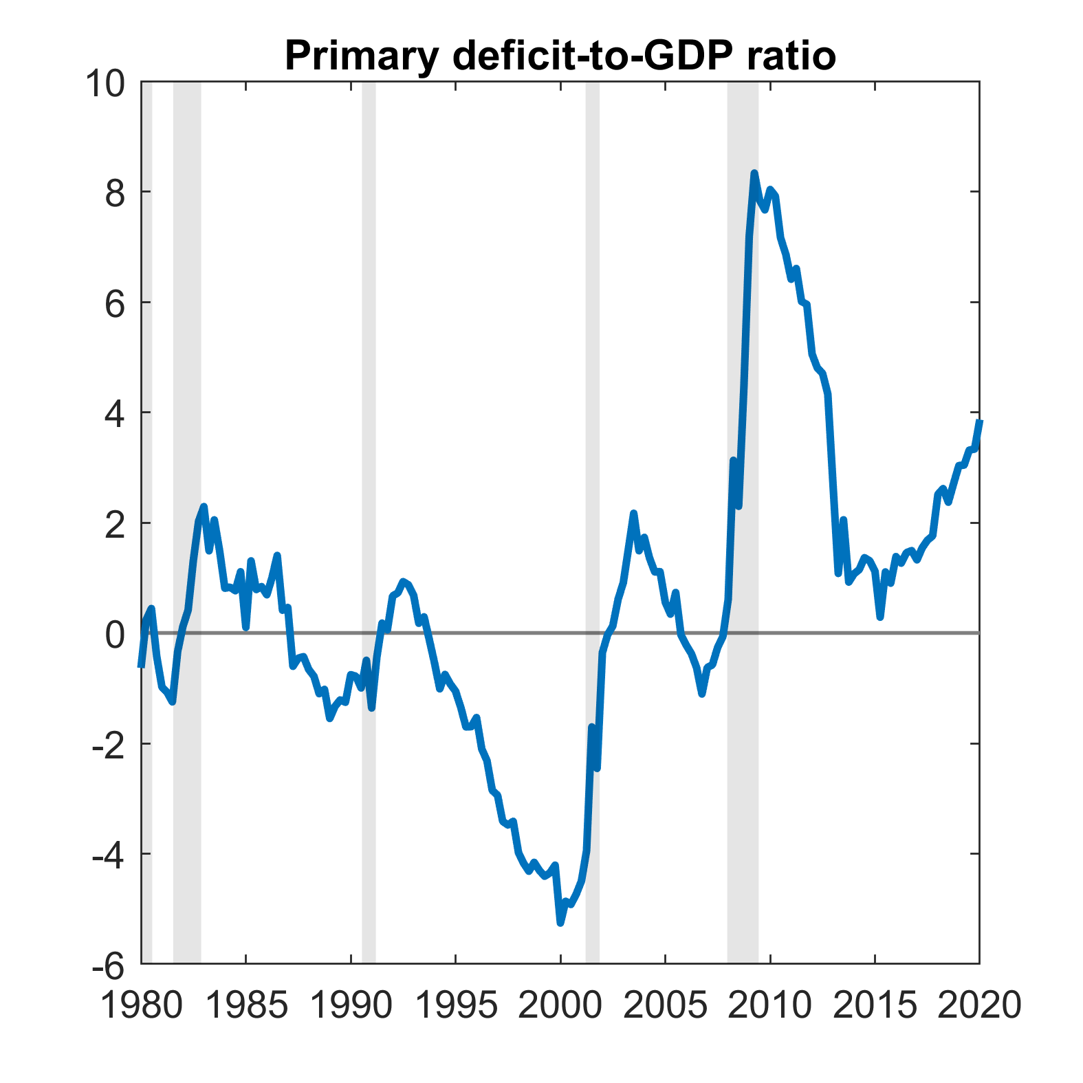
(a) Primary deficit to GDP ratio

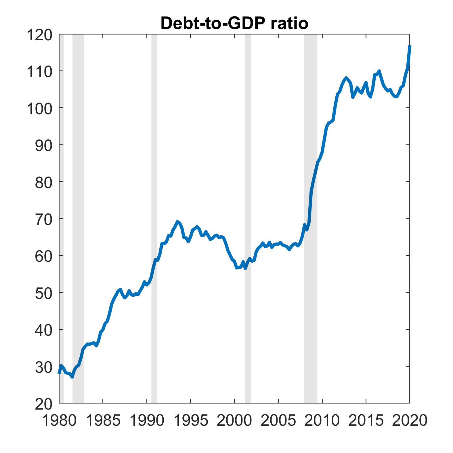
(b) Debt-to-GDP ratio

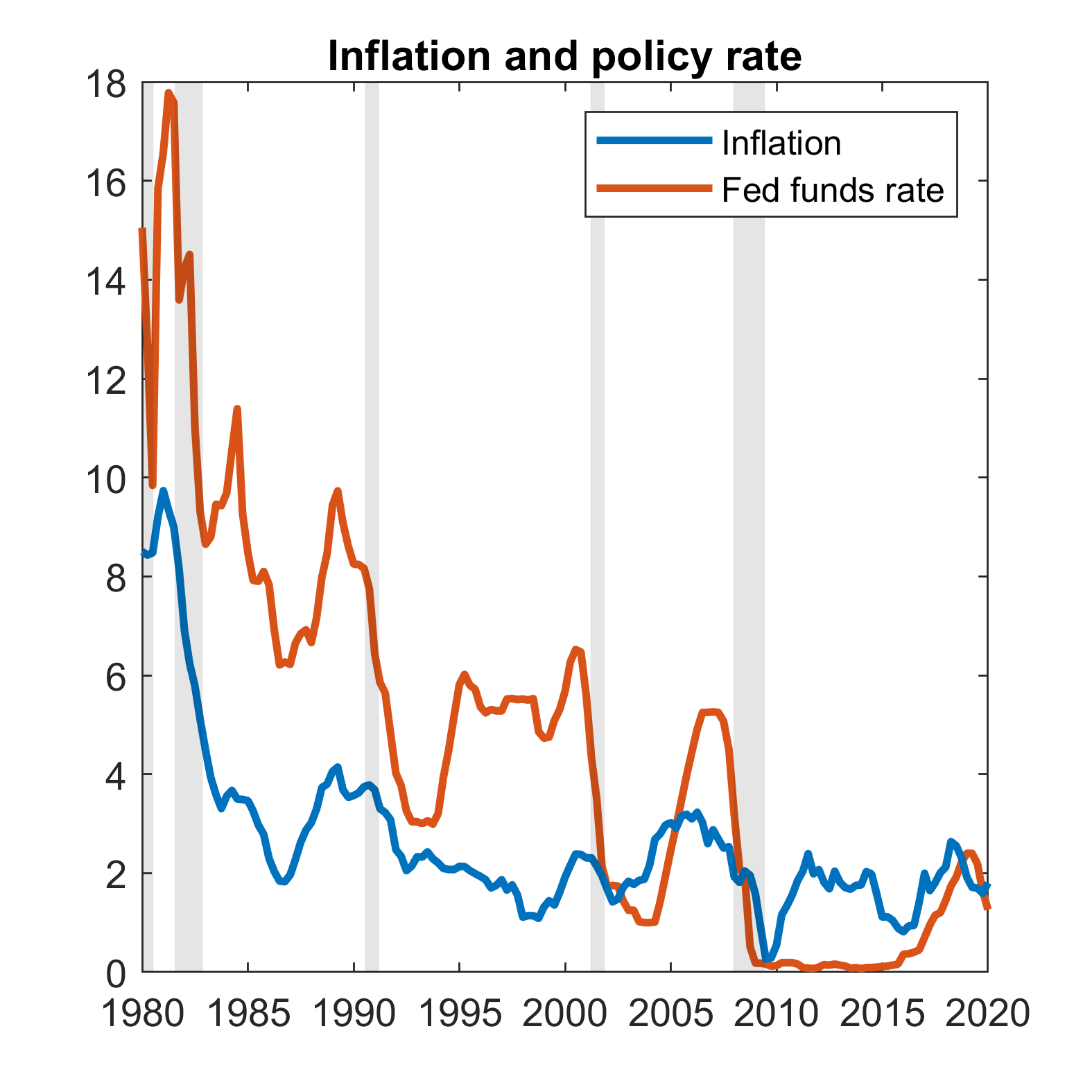
(c) Inflation and federal funds rate

Figure 1: The paths of the primary deficit to GDP ratio, debt-to-GDP ratio, inflation and policy rate in the U.S. Source: FRED database.

As a result, the Great Recession deteriorated the fiscal positions of most advanced economies. Figures 1a and 1b show the expansion in both the fiscal deficit and the debt-to-GDP ratio for the United States starting in 2008. Monetary policy also reacted promptly decreasing sharply the nominal interest rate to a level very close to zero (see Figure 1c). The level of inflation in the US rebounded after the initial drop and then started drifting down, remaining below target. Thus the US almost doubled the level of public debt from the pre-crisis level of about 60% in 2007 to a level above 110% in 2016. Other countries exhibit very similar dynamics, and the response to the crisis was clearly marked by an increase in public debt in most developed economies. In the euro area the increase in public debt triggered the sovereign debt crisis and a second recession. Evidently the government’s aim was to support the collapsing level of aggregate demand.

The increase in debt was brought about both by an increase in government spending and by a decrease in taxation. This boosted a large literature on fiscal multiplier, both spending and tax multipliers. Some works aimed at understanding the analytical mechanism of the fiscal multipliers, and its interaction with the zero lower bound (see Christiano et al., 2011; Eggertsson, 2011; Woodford, 2011). These works showed that multipliers for public spending are larger when the ZLB avoids the crowding out effect in private spending, thus amplifying the effect on output. When nominal interest rates are positive and adjust according to a Taylor rule, the rise in inflation that follows an expansion in government spending causes the central bank to raise the nominal interest rate to counteract the initial increase in demand. Conversely, when the ZLB constraint is binding the nominal interest rate does not raise to curb inflationary pressures, thus not dampening demand. Another strand of the literature focused on quantifying these multipliers empirically, using VARs, and theoretically, using DSGE models (e.g., Leeper et al., 2010; Ramey, 2011; Zubairy, 2014; Leeper et al., 2017; Ramey, 2019). Given the attention drawn by the Great Recession, many works investigated the possibility that fiscal multipliers vary depending on the state of the economy, and empirically investigates whether fiscal multipliers are higher during recessions than in normal times. The rational behind this assumption is that in a Keynesian world the economy will not always be characterized by full employment of resources, suggesting a higher multiplier during economic slack. The seminal paper by Auerbach and Gorodnichenko (2012) showed that fiscal multipliers are non-linear and state dependent. The papers by Blanchard and Leigh (2013, 2014) and its preceding Box in the IMF World Economic Outlook 2012 have been widely discussed, and have clearly influenced the policy debate and possibly the policy stance in some countries. These results are corroborated by many other works (Auerbach and Gorodnichenko, 2013; Caggiano et al., 2015; Fazzari et al., 2015). More recently, Ramey and Zubairy (2018) cast doubt on these results, because they estimate multipliers which are below one also during recession periods.

This very large literature investigates fiscal multipliers of both spending and different kinds of taxes. In this paper, we aim to fill a gap in this literature by instead analyzing the debt multiplier, that is, the output effect of a pure change in government debt, caused by the mere deferral of future taxes. This topic has acquired even greater importance in light of the COVID-19 epidemic. In fact, while the Fed and other central banks reacted to the adverse shock by bringing interest rates to zero once again, the governments of many affected countries implemented a number of tax relief and tax deferral measures. Analysing the effects of tax cuts and the interplay between the level of debt and the stance of monetary policy is a key issue in the current economic debate.

What are in general the effects of a temporary and pure change in government debt on economic activity? It is well known in the literature that, assuming lump-sum taxes, a standard infinitely-lived representative (ILRA) agent model provides a very simple and disarming answer to this question: none. Ricardian equivalence would hold in such a model, so the effect of deferring lump-sum taxes would affect the economy only if (and to the extent that) taxes are distortionary. It is also well-known that in an overlapping generations (OLG) framework, the Ricardian equivalence does not hold because taxes levied at different times affect different cohorts, thus a pure deferral of taxes has a positive impact on private aggregate demand. As such, an increase in the level of public debt, caused by a cut in lump-sum taxes, would have a positive effect on output. This is the effect we want to study. One could consider the debt multiplier as a complement to the fiscal multipliers so far appeared in the literature, mainly derived in an ILRA framework. The debt multiplier would be the additional multiplier that one can get if any temporary fiscal policy measure would be financed through a pure temporary increase in public debt (i.e., a postponement of lump-sum taxes). The aim of this paper is to analyze this debt multiplier.

Hence, we move away from the infinitely-lived representative agent (ILRA) assumption and adopt an OLG setting. In particular, we investigate two questions: (i) How does the debt multiplier depend on the level of public debt? (ii) Is the debt multiplier higher or lower in crisis time, that is, in a situation where there is a big negative demand shock so that the nominal interest rate hits the zero lower bound (ZLB)?

A clarification at this point is needed. What we call “debt multiplier”is similar to what is often referred to in the literature as “transfer multiplier”. Giambattista and Pennings (2017) and Mehrotra (2018) focus on the analysis of the transfer multiplier in two-agents models (respectively with a hand-to-mouth/Ricardians agents economy and with savers/borrowers consumers). Notably, these are alternative ways of breaking the Ricardian equivalence. By using a different denomination, we would like to stress the role of debt as a fiscal instrument, and the idea that government debt is households’ financial wealth, thus it is part of the supply of assets affecting the equilibrium real interest rate, as in Ascari and Rankin (2013).

Regarding question (i), in an ILRA framework the steady state real interest rate is pinned down by the subjective discount rate of the representative agent’s utility function. Instead, in an OLG framework the real interest rate also depends on the amount of assets in the economy. The larger the amount of assets, the higher will be the steady state real interest rate needed for the OLG agents to be willing to hold those assets. Since government bonds represent net wealth in an OLG framework, an increase in the level of debt means an increase in the level of the real interest rate at steady state. Question (ii) arises naturally from the literature on fiscal multipliers, that shows that fiscal multipliers are larger when the nominal interest rate is stuck at the ZLB.

This paper presents two lines of analysis. First, following Eggertsson (2011), we provide analytical results about the sign of the debt multiplier by considering a linearized version of a simple OLG model. Our findings indicate that the debt multiplier is positive even if the tax reduction is totally reversed in the future. We also find that debt multipliers increase with the level of debt, because of the positive relationship between fiscal multipliers and steady state real interest rates. Hence, the starting level of public debt affects the debt multiplier, especially so during a ZLB episode. In this respect, the calls for fiscal consolidation in recession times seem ill-advised. Second, to account for the presence of non-linear dynamics (see, Lindé and Trabandt, 2018), we take the model in its original non-linear form and run a series of simulation exercises to quantify the debt multiplier. In normal times, or in a period of mild recession in which nominal rates remain positive, the multiplier is generally quite small, unless we shut off the wealth effect channel of government debt on labor supply. The debt multiplier is larger when the recession is severe and interest rates drop to zero. This reinstates the importance of fiscal stimulus when conventional monetary policy is impotent. Quantitatively, three elements are important for the size of the debt multiplier: the average life length (i.e., the survival probability), the income effect on labor supply and the persistence of the debt expansion. If we set the survival probability to 0.95, use GHH preferences, and consider a permanent expansion in debt, the debt multipliers in our model is equal to 0.74 on impact, not too distant from the estimates of the government spending multipliers reported by the recent literature. Finally, we also show that a high steady state level of debt could provide monetary policy with more room for manoeuvre in case of a deflationary shock, because it increases the steady state nominal rate, through a rise in the steady state real rate, for any given steady state inflation target.

The paper is organized as follows. Section 2 presents some empirical evidence relating long-term real interest rates to the level of debt-to-GDP. Section 3 describes the OLG model using two different specifications for the preferences of households. Section 4 contains the analytical derivation of debt multipliers. Section 5 investigates numerically the size of multipliers and the relation with the level of debt. Section 6 concludes.

2 Stylized facts

One implication of the OLG framework is that the long-run debt-to-output ratio determines the long-term real interest rate. The larger is the level of debt, the higher the real interest rate. This is the key mechanism through which the level of debt affects the debt multiplier. The question whether government debt affects the real interest rate has often been investigated in the literature. One possible channel through which this can occur is capital stock. If government spending crowds out the physical capital stock, then, from a simple production model, an exogenous increase in government debt causes the real interest rate to increase. Moreover, factors other than government debt can influence the determination of interest rates in credit markets (see Engen and Hubbard, 2004).

The insurgence of the sovereign debt crisis in 2010 has posed also other interesting issues concerning the link between government debt and interest rate spreads. Intuitively, as one country’s government debt goes up, the perception of investors on the risk of investing in that particular country worsens, thus dampening demand for the country’s government bonds. This lowers the price of bonds and boosts risk premia and yields, which in turn makes the debt burden heavier. Then, the country may need to increase debt again to face higher interest payments, thus triggering a vicious cycle of higher debt and higher interest rates.

Figure 2 shows the long-term real interest rate and the government debt-to-GDP ratio for a set of countries. The long term interest rate is long-term government bond yield (in most cases 10 year) adjusted for inflation (calculated as the change in the GDP deflator). We use 2000-2018 averages to indicate steady state values. When average inflation is particularly high over the sample we incur in negative values for the real interest rate. The scatter plot captures the positive relationship between the two variables, as the regression line is positively sloped. The case of Greece is evident, with a high level of debt-to-GDP accompanied by a high real interest rate.

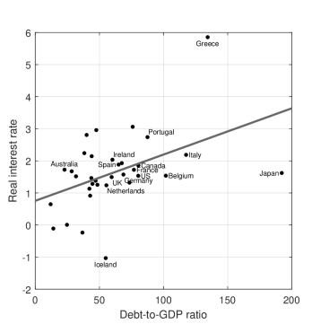
Figure 2: The relationship between debt-to-GDP ratio and the real interest rate (2000-2018 averages).

Thus, the empirical evidence suggests that the long-term real interest rate is positively related to the long-run level of debt as a percentage of GDP. In the remainder of the paper, we will show that this relationship holds also from a theoretical point of view.

3 The model

We use a dynamic general equilibrium model with overlapping generations à la Blanchard (1985). Agents have an exogenous probability, $q$ ($0<q<1$), of surviving to the next period. This framework includes infinite lives as a special case, namely where $q=1$. Apart from the characteristics concerning specifically overlapping generations we keep the model as simple as we can and comparable to the standard infinitely lived agents model of Eggertsson (2011).

3.1 Households

The setup is very similar to Ascari and Rankin (2013). Households maximize utility in consumption and leisure. They receive income from working, from interests on bonds and from profits. At the same time, they allocate their income stream between consumption and bond holdings, and they pay lump-sum taxes.

As a benchmark case, we consider the following log-log utility function:

$$E_{n}\sum_{t=n}^{\infty}\left(\beta q\right)^{t-n}\xi_{t}\left[\log\left(C_{s,t}\right)+\eta\log\left(1-L_{s,t}\right)\right]\text{,}$$ (1)

where $n$ is the current period and $s$ ($\leq n$) is the household’s birth-period. $C_{s,t}$ denotes consumption in period $t$ of a household born in period $s$ and likewise for hours worked $L_{s,t}$. $\beta>0$ is the discount factor, $\xi_{t}$ is a shock to preferences or to the discount factor and $\eta>0$. In equilibrium a positive realization of $\frac{\xi_{t+1}}{\xi_{t}}$ will induce a rise in the effective discount factor so that households want to save more. This will trigger a fall in consumption today and lead to an economic recession which could imply zero nominal interest rates.

The optimization problem of the households consists of maximizing the utility function subject to the budget constraint:

$$P_{t}C_{s,t}+B_{s,t}^{N}=(1/q)\left(1+i_{t-1}\right)B_{s,t-1}^{N}+W_{t}L_{s,t}+P_{t}\left(D_{t}-T_{t}\right)\text{.}$$ (2)

$B_{s,t}^{N}$ are bond holdings of a household born in period $s$ in period $t$. $P_{t}$, $W_{t}$ and $i_{t}$ indicate the price index, wage and the nominal interest rate, respectively. $D_{t}$ and $T_{t}$ denote profits from firms and lump-sum taxes. As in Blanchard (1985), the households receive an “annuity” at the gross rate $1/q$ on their financial wealth if they survive, otherwise this wealth passes to the insurance company. The profits of the insurance companies are zero in equilibrium.

From the first order conditions we obtain the following in the benchmark case:

$$\frac{W_{t}}{P_{t}} =\eta\frac{C_{s,t}}{1-L_{s,t}}\text{,}$$ (3)

$$C_{s,t} =E_{t}\left\{\frac{C_{s,t+1}}{\beta\left(1+r_{t}\right)}\frac{\xi_{t}}{\xi_{t+1}}\right\}\text{,}$$ (4)

where $\left(1+r_{t}\right)=\left(1+i_{t}\right)P_{t}/E_{t}P_{t+1}$ is the real interest rate. Equation (3) is the individual labor supply, while equation (4) is the individual Euler equation.

In this case the utility function implies the existence of a wealth effect between hours and consumption. Although the benchmark specification of the utility function is standard in OLG models, it implies that as agents age they will hit the constraint of non-negative labor supply, because $C_{s,t}$ increases with the agent’s age, $t-s$. Hence, we consider also the case where this effect is absent, through the use of Greenwood et al. (1988) (henceforth, GHH) preferences. Moreover, the wealth effect on labor supply has strong effects on the fiscal multipliers in DSGE models, so that the literature often employs similar type of preferences (e.g., Monacelli and Perotti, 2008). In the GHH case we have:

$$E_{n}\sum_{t=n}^{\infty}\left(\beta q\right)^{t-n}\xi_{t}\log\left[C_{s,t}-\left(\eta/\varepsilon\right)L_{s,t}^{\varepsilon}\right]\text{,}$$ (5)

where $\varepsilon>1$. GHH preferences enables to avoid this problem as (3) is replaced by the following:

$$\frac{W_{t}}{P_{t}}=\eta L_{s,t}^{\varepsilon-1}\text{,}$$ (6)

where there is no $C_{s,t}$ and thus the labor supply is independent of $s$. At the same time (4) is replaced by:

$$C_{s,t}-\left(\eta/\varepsilon\right)L_{s,t}^{\varepsilon}=E_{t}\left\{\frac{C_{s,t+1}-\left(\eta/\varepsilon\right)L_{s,t+1}^{\varepsilon}}{\beta\left(1+r_{t}\right)}\frac{\xi_{t}}{\xi_{t+1}}\right\}.$$ (7)

Aggregation.

We can derive the aggregate counterpart of equations (3) and (4) by multiplying by $\left(1-q\right)q^{t-s}$ (individuals born in period $s$ and still alive in $t$) and summing both sides for $s=-\infty,...,t$. The relationship between a generic aggregate variable $X_{t}$ and its constituent individual variables is:

$$X_{t}=\sum_{s=t}^{-\infty}\left(1-q\right)q^{t-s}X_{s,t}\text{.}$$ (8)

After some algebra we obtain the following aggregate expressions:

$$\frac{W_{t}}{P_{t}}\left(1-L_{t}\right) =\eta C_{t}\text{,}$$ (9)

$$E_{t}C_{t+1}+\frac{\left(1-q\right)}{\left(1+\eta\right)q}\frac{V_{t}}{E_{t}\delta_{t+1}} =\beta E_{t}\left\{\left(1+r_{t}\right)\frac{\xi_{t+1}}{\xi_{t}}\right\}C_{t},$$ (10)

where $\delta_{t}=1+q\beta E_{t}\left\{\frac{\xi_{t+1}}{\xi_{t}}\delta_{t+1}\right\}$. Note that for $q<1$, government debt represents net wealth and thereby affects consumption spending. Following Ascari and Rankin (2013), we define financial wealth as: $V_{s,t}=\frac{1}{q}\left(1+i_{t}\right)B_{s,t}^{N}$. Note that the relationship of aggregate to individual financial wealth is slightly different from the general one, being rather: $\frac{1}{q}V_{t}=\sum_{s=t}^{-\infty}\left(1-q\right)q^{t-s}V_{s,t}$, because we include the annuity payout in our definition of $V_{s,t}$. The aggregate Euler equation says that the growth rate of aggregate consumption depends positively on the real interest rate, on the growth rate of the shock and negatively on aggregate financial wealth.

For the model with GHH preferences (9) and (10) become:

$$\frac{W_{t}}{P_{t}} =\eta L_{t}^{\varepsilon-1},$$ (11)

$$E_{t}C_{t+1}+\frac{\left(1-q\right)}{q}\frac{V_{t}}{E_{t}\delta_{t+1}}-\left(\eta/\varepsilon\right)E_{t}L_{t+1}^{\varepsilon} =\beta E_{t}\left\{\left(1+r_{t}\right)\frac{E_{t}\xi_{t+1}}{\xi_{t}}\right\}\left[C_{t}-\left(\eta/\varepsilon\right)L_{t}^{\varepsilon}\right].$$ (12)

Finally, the representative households decides how to allocate its consumption expenditures among the different varieties of goods, indexed by $i\in\left[0,1\right]$. The consumption index is represented by a standard CES function:

$$C_{s,t}=\left[\int\limits_{0}^{1}C_{i,s,t}^{\frac{\theta-1}{\theta}}di\right]^{\frac{\theta}{\theta-1}},$$ (13)

with $\theta>1$. The household maximizes (13) subject to the budget constraint $\int\limits_{0}^{1}P\left(i\right)C\left(i\right)_{s,t}di=Z_{s,t}$, where $Z_{s,t}$ is total expenditure for goods. This leads to the familiar constant elasticity demand function for good type $i$:

$$C_{i,s,t}=\left(\frac{P_{i,t}}{P_{t}}\right)^{-\theta}\frac{Z_{s,t}}{P_{t}}=\left(\frac{P_{i,t}}{P_{t}}\right)^{-\theta}C_{s,t},$$ (14)

where

$$P_{t}=\left[\int\limits_{0}^{1}P_{i,t}^{1-\theta}di\right]^{\frac{1}{1-\theta}}.$$ (15)

3.2 Firms

The problem of firms is independent of households’ preferences. There is a continuum of firms indexed by $i\in\left[0,1\right]$, each producing a differentiated good. All firms operate under monopolistic competition and use the same technology represented by a Cobb-Douglas production function with aggregate labor as unique factor of production, so we have that $Y_{i,t}=L_{i,t}^{\sigma}$ where $Y_{i,t}$ and $L_{i,t}$ are the output and the amount of labor employed by firm $i$. Firms face the same demand schedule and take $P_{t}$, $W_{t}$ and $Y_{t}$ as given.

Prices are sticky à la Calvo (1983), so that each firm may reset its price only with a probability $1-\alpha$ in any given period. With probability $\alpha$ it keeps its price unchanged. The optimization problem of a firm $i$ that adjusts its price $P_{i,n}$ in period $n$ is then:

$$\max_{P_{i,n}}E_{n}\sum_{t=n}^{\infty}\alpha^{t-n}\Delta_{n,t}\frac{P_{i,n}Y_{i,t}-W_{t}L_{i,t}}{P_{t}}$$ (16)

subject to the demand schedule

$$Y_{i,t}=\left(\frac{P_{i,t}}{P_{t}}\right)^{-\theta}Y_{t}\text{,}$$ (17)

where the discount factor $\Delta_{n,t}$ is given by

$$\Delta_{n,t}\equiv\left(1+r_{n}\right)^{-1}\left(1+r_{n+1}\right)^{-1}...\left(1+r_{t-1}\right)^{-1}\text{, \ \ \ }\Delta_{n,n}\equiv 1.$$ (18)

If we define $P^{*}_{n}$ as the new price set in period $n$ by firm $i$, solving the optimization problem yields the following result:

$$P^{*}_{n}=E_{n}\left[\frac{\theta}{\theta-1}\frac{1}{\sigma}\frac{\sum_{t=n}^{\infty}\alpha^{t-n}\Delta_{n,t}W_{t}Y_{t}^{\frac{1}{\sigma}}P_{t}^{\frac{\theta}{\sigma}-1}}{\sum_{t=n}^{\infty}\alpha^{t-n}\Delta_{n,t}Y_{t}P_{t}^{\theta-1}}\right]^{\frac{1}{1+\frac{\theta}{\sigma}-\theta}}\text{.}$$ (19)

This expression says that the new price depends on current and expected future values of aggregate output, the general price level and the wage level. All firms resetting their prices in period $n$ will choose the same new price.

3.3 Government

The government’s budget constraint in nominal terms is:

$$P_{t}\left(G_{t}-T_{t}\right)+i_{t-1}B_{t-1}^{N}=\left(B_{t}^{N}-B_{t-1}^{N}\right)\text{,}$$ (20)

where $G_{t}$ is public spending. In real terms we obtain:

$$G_{t}-T_{t}=B_{t}-(1+r_{t-1})B_{t-1}\text{,}$$ (21)

where we defined $B_{t}=B_{t}^{N}/P_{t}$. Then, in line with Ascari and Rankin (2013), we express the government budget constraint in terms of the real government debt inclusive of interest payments, which we denote as $B_{t}^{\prime}=(1+r_{t})B_{t}$:

$$G_{t}-T_{t}=(1+r_{t})^{-1}B_{t}^{\prime}-B_{t-1}^{\prime}\text{.}$$ (22)

Clearly only two of the three policy instrument can be chosen independently. In what follows we will consider exogenous fiscal shocks to government debt, thus leaving lump-sum tax $T_{t}$ to be determined implicitly by (22) as residual.

The central bank follows a standard contemporaneous Taylor rule if the nominal interest rates is positive. Otherwise it is constrained by the zero lower bound (see equation (26)).

3.3.1 Market clearing

Equilibrium in the goods market simply requires that:

$$Y_{t}=C_{t}+G_{t}\text{.}$$ (23)

4 Analytical investigation of debt multipliers

In this section, we present the reduced form solution and we explain the solution method to derive the multipliers for government debt. First, we derive the multipliers in a positive interest rates environment, where the monetary authority follows a Taylor rule. Second, we present the multipliers in a zero interest rates context.

4.1 Model solution

4.1.1 Benchmark case

We derive a simplified version of the model after log linearizing the model so that a generic variable $X_{t}$ can be approximated by $x_{t}=\frac{X_{t}-X}{X}\simeq\log\left(\frac{X_{t}}{X}\right)$.The following equations are the dynamic AD curve (24), the New Keynesian Phillips Curve (25), the Central bank rule for nominal interest rates (26) and the dynamics of the auxiliary variable $\delta_{t}$ (27):

$$E_{t}y_{t+1} =\beta(1+\bar{r})y_{t}+\beta(1+\bar{r})\left(i_{t}-E_{t}\pi_{t+1}\right)+E_{t}g_{t+1}-\beta(1+\bar{r})g_{t}$$ (24)

$$-\beta(1+\bar{r})r_{t}^{e}-\left[\beta(1+\bar{r})-1\right]b_{t}^{\prime}+\left[\beta\left(1+\bar{r}\right)-1\right]E_{t}\hat{\delta}_{t+1}\text{,}$$

$$\pi_{t} =\left(1+\bar{r}\right)^{-1}E_{t}\pi_{t+1}+\kappa\left[y_{t}-\left(1-L\right)\sigma g_{t}\right]\text{,}$$ (25)

$$i_{t} =\max(0,r_{t}^{e}+\phi_{\pi}\pi_{t}+\phi_{y}y_{t})\text{,}$$ (26)

$$\hat{\delta}_{t} =q\beta\hat{\delta}_{t+1}-q\beta\left[r_{t}^{e}-\log\left(1+\bar{r}\right)\right],$$ (27)

where we define $r_{t}^{e}=\log\left(1+\bar{r}\right)-\Delta\hat{\xi}_{t+1}$, following Eggertsson (2011), and

$$\kappa=(1-\alpha)\left[\alpha^{-1}-\left(1+\bar{r}\right)^{-1}\right]\left(1-\theta+\frac{\theta}{\sigma}\right)^{-1}\frac{1}{1-L}\frac{1}{\sigma}.$$

Parameters $\phi_{\pi}$ and $\phi_{y}$ are the responses of the nominal interest rate to inflation and output, respectively. Moreover, $\bar{r}$ is the steady state value of the real interest rate, which is derived endogenously and corresponds to:

$$\bar{r}=\frac{q\left(1+\eta\right)}{\beta q\left(1+\eta\right)-\left(1-q\right)\left(1-\beta q\right)\frac{B}{Y}}-1\text{.}$$ (28)

This expression states that the steady state real interest rate, and consequently the equilibrium solution, depends on the probability of surviving and on the steady state debt to output ratio. (28) implies that a larger steady state debt-to-GDP level causes a higher level of the steady state real interest rate, which is consistent with the empirical evidence showed in Section 2. The reason is the following. Agents are born with zero financial wealth, so they must accumulate it during their lifetime. In each period, thus, aggregate wealth drags on consumption growth in the aggregate Euler equation (10) in the Blanchard (1985) OLG framework, because the agents that die in each period consume more that the one that are born (some works in the literature refer to this effect as “generational turnover effect”). This has two important implications. First, the real interest rate, that keeps aggregate consumption in steady state constant, is larger than the one that would keep the individual consumption constant in steady state. According to (4), the latter is the same as in the ILRA model and equal to $(1/\beta-1)$. Hence, differently from ILRA models, the following holds:

$$\beta\left(1+\bar{r}\right)>1\text{.}$$ (29)

Given (4), condition (29) implies that agents save and accumulate wealth during their lifetime, exactly because the real interest rate is larger than the subjective discount rate.

Second, the steady state real interest rate, $\bar{r}$, depends on financial wealth, i.e., on the supply of assets in the economy. The larger the amount of assets, the stronger the generational turnover effects and the larger should be the real interest rate to keep aggregate consumption constant. In simpler words, the supply and demand of assets determine the steady state real interest rate in this OLG framework, so that the larger the supply of assets in the economy the higher should be the real interest rate to make agents willing to hold that amount of assets.

This relationship has important implications for the model solution and we will come back to it in what follows. For the moment, it is important to stress that the steady state value of the debt affects the steady state real interest rate, and hence it affects the dynamics of the economy and, as we will show, the multipliers.

We consider temporary shocks. In computing the fiscal multipliers, we follow the same approach in Eggertsson (2011) to which thus our results are immediately comparable. To do so, we make the following assumptions. We define the long-run as the time at which the shock $r_{t}^{e}$ is at steady state. The short-run is the period in which the economy is subject to temporary disturbances and it is defined by $r_{t}^{e}=r_{S}^{e}$. This shock reverts back to steady state with probability $(1-\mu)$. A negative realization of $r_{t}^{e}$ implies that households want to save more so that the real interest rate must decline to keep output constant. In general it can be interpreted as any exogenous reason for a decline in spending. Eggertsson (2011) suggests it can be thought for example as an exogenous increase in the probability of default by borrowers, which characterizes a banking crisis. As in Eggertsson (2011), we assume that fiscal policy is perfectly correlated with the shock, that is, we consider government debt increases/decreases which are a direct reaction to the shock, such that $b_{t}^{\prime}=b_{S}^{\prime}$ in the short run and $b_{t}^{\prime}=0$ in the long run (meaning that in the long-run $B_{t}^{\prime}$ is back to the steady state). Here we also implicitly assume that, for a given change in government debt, government spending remains constant at its steady state and all the adjustment occurs through a change in taxation.

Expectations about a generic variable $x_{t}$ (in deviation from its steady state) are formed as follows:

$$E_{t}x_{t+1}=\mu E^{S}_{t}x_{t+1}^{S}+\left(1-\mu\right)0=\mu E^{S}_{t}x_{t+1}^{S},$$ (30)

where $S$ stands for “short run”. The notation $E^{S}_{t}$ is used as the expectation of the variable $x_{t+1}$ conditional on the shock being in the short run state. Accordingly, $x_{t+1}^{S}$ is the value of $x_{t+1}$ conditional on the short run state. When the system is back to the steady state the variable is equal to its steady state value, so that the deviation from the steady state is zero. This applies to all the variables in the model.

The model can be solved through standard methods, such as the method of undetermined coefficients. The solution of the model enables to determine an algebraic expression for the multipliers of government spending and debt.

4.2 Positive interest rates

In this section we analyze a debt increase when interest rates are positive. In this case, a standard Taylor rule describes monetary policy: a negative realization of the shock $r_{t}^{e}$ prompts the reaction of the central bank that cuts nominal rates to counteract the fall in output and inflation. However, nominal rates remain positive as the shock $r_{t}^{e}$ is too small to activate the ZLB constraint.

We assume that government spending remains constant at its steady state. In the short run taxes will adjust (decrease) in order to meet the government budget constraint, implying a positive (higher than the steady state) level of debt. Given the way expectations are formed, when the shock is switched off, it is implicitly assumed that debt has to go back to its initial steady state level. Otherwise, the steady state will be different from the initial one, and that is not consistent with (30). Again the adjustment occurs through an increase in taxation. The impact government debt multiplier is:

$$BM=\frac{\left[\beta(1+\bar{r})-1\right]\left[1-(1+\bar{r})^{-1}\mu\right]}{\left[\beta(1+\bar{r})\left(1+\phi_{y}\right)-\mu\right]\left[1-(1+\bar{r})^{-1}\mu\right]+\beta(1+\bar{r})\kappa\left(\phi_{\pi}-\mu\right)}.$$ (31)

Note that, given that $0<\mu<1$ and $\beta(1+\bar{r})>1$, the effect of an increase in government debt is always positive if $\phi_{\pi}-\mu>0$, which is likely to occur in standard models where the Taylor principle ($\phi_{\pi}>1$) holds. In the case of a tax reduction, the increase in debt shifts out aggregate demand, stimulating production. Private consumption actually increases because in an OLG framework agents will experience a positive wealth effect, as they could be dead when taxes will adjusts upwards. The rise in consumption thus implies a higher demand and, in turn, higher output, because of nominal rigidities. Labor demand shifts upwards, because those firms which cannot adjust prices due to nominal rigidities produce more to cope with the increase in demand. While the positive wealth effect stimulates household consumption, it also reduces labour supply. Despite the shift in labor supply, the net effect is however positive for output. Note that in case of ILRA, private consumption will instead not respond because Ricardian equivalence holds. Indeed, the solid blue line in Figure 3 shows that the debt multiplier depends on the probability of surviving $q$ and it is equal zero when $q=1$.

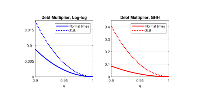
Figure 3: The debt multiplier for different values of the probability of survival.
Notes: Analytic multipliers for the baseline calibration, see Table 5.

However, the multiplier is lower than one, that is, the effect of debt on output is less than proportional, since $\mu<1$ and $\phi_{\pi}-\mu>0$. Moreover, the multiplier is lower when the responses of monetary policy to both output ($\phi_{y}$) and inflation ($\phi_{\pi}$) are stronger. This is very intuitive, because the increase in debt will cause, ceteris paribus, an increase both in output and inflation, and then the more monetary policy responds to them, the lower will be the debt multiplier. The monetary policy response following a Taylor rule is partially crowding out the expansionary effects of an increase in debt, and the more so the more hawkish is monetary policy.

Last, but not least, the debt multiplier depends on $\bar{r}$, and hence it depends on the value of debt. This result has been neglected in the literature, and it arises naturally in an OLG framework, and it holds for any fiscal multiplier, not only the debt one. The solid blue line in Figure 4 shows that the debt multiplier increases with the level of debt. The coefficient on $b^{\prime}_{t}$ on the RHS of (24), which derives from (10), is an increasing function of $\bar{r}$, so that the effect of a change in $b^{\prime}_{t}$ increases with the level of debt-to-gdp ratio. The intuition of this channel comes form the fact that in an OLG framework agents are saving during their lifetimes. Indeed, this coefficient in (24) is positive exactly because condition (29) holds, as explained earlier. A temporary increase in the level of debt determines a temporary increase in the real interest rate. According to (4), agents are saving because the steady state real interest rate is larger then the subjective discount rate. However, a given marginal increase in the real interest rate would determine a lower response of savings (and a higher response of current consumption), the higher the starting (steady state) level of real interest rate, because the marginal utility is decreasing. In other words, the higher the steady real interest rate, the higher the rate of growth of individual consumption and hence the distance between the marginal utility between two consecutive periods. Hence, for a given temporary change in the real interest rate, agents will allocate the positive wealth effect due to an increase in the debt level relatively more to current consumption than to savings.

The multiplier of government debt is zero for the ILRA model under positive interest rates. In fact, in this case, $(1+\bar{r}=\beta)$, Ricardian equivalence holds and government debt plays no role in stimulating demand.

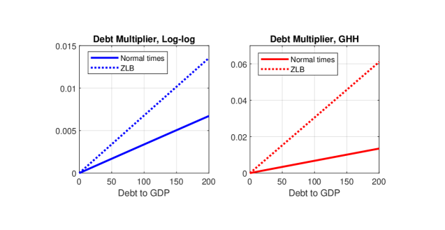
Figure 4: The debt multiplier for different values of the debt-to-GDP ratio.
Notes: Analytic multipliers for the baseline calibration.

4.2.1 GHH preferences

We do the same exercise with the model characterized by GHH preferences. Equations (24) and (25) become:

$$\frac{1}{\theta}E_{t}y_{t+1} =\beta(1+\bar{r}_{GHH})\frac{1}{\theta}y_{t}+\frac{\beta(1+\bar{r}_{GHH})}{\zeta}\left(i_{t}-E_{t}\pi_{t+1}\right)$$ (32)

$$+E_{t}g_{t+1}-\beta(1+\bar{r}_{GHH})g_{t}-\frac{\left[\beta(1+\bar{r}_{GHH})-1\right]}{\zeta}b_{t}^{\prime}$$

$$-\frac{\beta(1+\bar{r}_{GHH})}{\zeta}r_{t}^{e}+\frac{\left[\beta(1+\bar{r}_{GHH})-1\right]}{\zeta}E_{t}\hat{\delta}_{t+1},$$

$$\pi_{t} =(1+\bar{r})^{-1}E_{t}\pi_{t+1}+\kappa_{GHH}y_{t},$$ (33)

where $\kappa_{GHH}=\left(1-\alpha\right)\left[\alpha^{-1}-(1+\bar{r})^{-1}\right](1-\theta+\theta/\sigma)^{-1}\left(\frac{\varepsilon}{\sigma}-1\right)$ and $\zeta=\frac{1}{1-\sigma/\varepsilon\left(1-1/\theta\right)}>1$. The relation between the steady state real interest rate and the debt-to-GDP ratio changes and it is now equal to:

$$\bar{r}_{GHH}=\frac{1}{\beta}\left[\frac{q\left[\varepsilon\theta-\sigma\left(\theta-1\right)\right]}{q\left[\varepsilon\theta-\sigma\left(\theta-1\right)\right]-\varepsilon\theta\left(1-q\right)\left(1/\beta-q\right)\frac{B}{Y}}\right]-1,$$ (34)

while the multiplier for debt becomes:

$$BM_{GHH}=\frac{\left[1-(1+\bar{r}_{GHH})^{-1}\mu\right]\left[\beta(1+\bar{r}_{GHH})-1\right]}{\frac{\zeta}{\theta}\left[\beta(1+\bar{r}_{GHH})\left(1+\frac{\theta}{\zeta}\phi_{y}\right)-\mu\right]\left[1-(1+\bar{r}_{GHH})^{-1}\mu\right]+\beta(1+\bar{r}_{GHH})\kappa_{GHH}\left(\phi_{\pi}-\mu\right)}.$$ (35)

Also in this case, we can prove numerically that the size of the multiplier is lower than one for sensible calibrations of the parameters.

Figure 3 and 4 show that the multiplier under GHH preferences is higher than under the benchmark log-utility preferences under our benchmark calibration in Table 5. This is due to complementarity between hours and consumption, which is higher under GHH preferences, as there is no wealth effect. Under benchmark preferences, the wealth effect due to the increase in the debt induces households to consume more and work less: the labor supply curve shifts inwards, and therefore mitigates the effects of the fiscal expansion. If households have GHH preferences, the wealth effect on labor supply is absent, thus the labor supply schedule is unaffected, leading to larger increases in hours, consumption and output.

4.3 Zero interest rates

We now turn the attention to the case where the zero lower bound constraint is binding. This occurs for big enough realizations of the shock $r_{t}^{e}$, precisely when $r_{t}^{e}<-\left(\phi_{\pi}\pi_{t}+\phi_{y}y_{t}\right)$, which implies:

$$i_{t}=0\text{.}$$ (36)

We make the same fiscal experiments presented under positive interest rates. For the benchmark model, the multiplier of government debt is modified as follows:

$$BM^{ZLB}=\frac{\left[\beta(1+\bar{r})-1\right]\left[1-(1+\bar{r})^{-1}\mu\right]}{\left[\beta(1+\bar{r})-\mu\right]\left[1-(1+\bar{r})^{-1}\mu\right]-\beta(1+\bar{r})\kappa\mu}$$ (37)

The multiplier is positive if:

$$\left[\beta(1+\bar{r})-\mu\right]\left[1-(1+\bar{r})^{-1}\mu\right]-\beta(1+\bar{r})\kappa\mu>0$$

Note that this condition crucially depends on the persistence of the shock $\mu$.

Under GHH preferences, we get the following zero lower bound multiplier:

$$BM_{GHH}^{ZLB}=\frac{\left[1-(1+\bar{r}_{GHH})^{-1}\mu\right]\left[\beta(1+\bar{r}_{GHH})-1\right]}{\left[1-(1+\bar{r}_{GHH})^{-1}\mu\right]\left[\beta(1+\bar{r}_{GHH})-\mu\right]\frac{\zeta}{\theta}-\mu\beta(1+\bar{r}_{GHH})\kappa_{GHH}}$$ (38)

The literature robustly finds that fiscal multipliers are higher under the ZLB than under positive interest rates. Our results make no exception, because this also holds for the debt multipliers in the OLG context for both specifications of preferences. While Figure 4 shows it numerically for our benchmark calibration, it is easy to show it analytically. Under benchmark preferences, the condition for the debt multiplier to be higher under the ZLB than when nominal rates are positive is:

$$\begin{split}\left[\beta(1+\bar{r})\left(1+\phi_{y}\right)-\mu\right]&\left[1-(1+\bar{r})^{-1}\mu\right]+\beta(1+\bar{r})\kappa\left(\phi_{\pi}-\mu\right)\\ &>\left[\beta(1+\bar{r})-\mu\right]\left[1-(1+\bar{r})^{-1}\mu\right]-\beta(1+\bar{r})\kappa\mu,\end{split}$$ (39)

which always holds as $\phi_{y}\geqslant 0$ and $\phi_{\pi}\geqslant\mu$. Similarly, with GHH preferences the corresponding condition is:

$$\begin{split}&\left[1-(1+\bar{r}_{GHH})^{-1}\mu\right]\left[\beta(1+\bar{r}_{GHH})-\mu\right]\frac{\zeta}{\theta}-\mu\beta(1+\bar{r}_{GHH})\kappa_{GHH}\\ &\quad<\frac{\zeta}{\theta}\left[\beta(1+\bar{r}_{GHH})\left(1+\frac{\theta}{\zeta}\phi_{y}\right)-\mu\right]\left[1-(1+\bar{r}_{GHH})^{-1}\mu\right]+\beta(1+\bar{r}_{GHH})\kappa_{GHH}\left(\phi_{\pi}-\mu\right),\end{split}$$ (40)

which is always satisfied as $\phi_{y}\geqslant 0$, $\theta,\zeta>1$ and $\phi_{\pi}\geqslant\mu$.

Intuitively, monetary policy is not reacting to inflation under the ZLB, so that there is no partial crowding out of the initial increase in aggregate demand. As shown in Eggertsson (2011), when nominal interest rates are zero the AD curve shifts from downward sloping, as it is standard in macroeconomic textbooks, to upward sloping, because the central bank does not offset inflationary pressures with interest rates hikes. In this case, a higher inflation means a lower real interest rate, thus implying higher demand. This is the reason why fiscal multipliers are bigger under the ZLB constraint.

4.4 Determinacy properties and the multipliers

The determinacy properties of the equilibrium for both models considered is crucially dependent on parameter $\mu$, i.e. on the probability of remaining out of the steady state after the shock. In general, the determinacy conditions, under both positive and zero interest rates and under both types of preferences, correspond to the conditions for the multipliers to be positive. It is important to note that, for both types of preferences under positive interest rates, the determinacy conditions are always satisfied if the Taylor principle holds. These conditions for the benchmark model and GHH preferences are respectively:

$$\mu^{2}+\beta(1+\bar{r})^{2}\left(1+\phi_{y}+\kappa\phi_{\pi}\right)-(1+\bar{r})\left[\beta\left(1+\phi_{y}+\kappa(1+\bar{r})\right)+1\right]\mu>0,$$ (41)

$$\mu^{2}+\frac{\beta(1+\bar{r}_{GHH})^{2}\theta}{\zeta}\left\{\frac{\zeta}{\theta}+\phi_{y}+\kappa\phi_{\pi}\right\}-(1+\bar{r}_{GHH})\left\{\frac{\beta\theta}{\zeta}\left[\frac{\zeta}{\theta}+\phi_{y}+(1+\bar{r}_{GHH})\kappa_{GHH}\right]+1\right\}\mu>0.$$ (42)

After some algebra, it can be shown that the denominators of $BM$ and $BM_{GHH}$ are positive if conditions (41) and (42) are verified, respectively. And, given that the numerators of $BM$ and $BM_{GHH}$ are always positive, this corresponds also to have positive multipliers for debt, thus implying that a debt increase leads to an output increase (and vice versa).

Interestingly, under zero interest rates, the determinacy conditions correspond again to the conditions for the multipliers to be positive, but in this case they are not satisfied for all values of $\mu$. The determinacy conditions in this case for the benchmark model and GHH preferences are respectively:

$$\mu^{2}-(1+\bar{r})\left\{\beta\left[1+\kappa(1+\bar{r})\right]+1\right\}\mu+\beta(1+\bar{r})^{2}>0$$ (43)

$$\mu^{2}-(1+\bar{r}_{GHH})\left\{\frac{\beta\theta}{\zeta}\left[\frac{\zeta}{\theta}+(1+\bar{r}_{GHH})\kappa_{GHH}\right]+1\right\}\mu+\beta(1+\bar{r}_{GHH})^{2}>0.$$ (44)

Given a standard calibration (see Table 5), under the benchmark model, the condition of determinacy is satisfied if $\mu\leqslant 0.70$. For these values of $\mu$ the positive relationship between the fiscal variables and output is confirmed. This condition on $\mu$ is even tighter under GHH preferences: for the same calibration, in this case $\mu$ should be $\leqslant 0.58$ for the system to be determined. Again, this condition also establishes that the multipliers are positive.

4.5 Government spending multipliers

Despite not being the main focus of the paper, we briefly report here the government spending multipliers. These multipliers regard a change in government spending at balance budget, that is, coupled with an one-off change in taxation and holding the public debt constant. For the benchmark case, the government spending multiplier is:

$$GSM=\frac{\left[\beta(1+\bar{r})-\mu\right]\left[1-(1+\bar{r})^{-1}\mu\right]+\beta(1+\bar{r})\kappa\left(1-L\right)\sigma\left(\phi_{\pi}-\mu\right)}{\left[\beta(1+\bar{r})\left(1+\phi_{y}\right)-\mu\right]\left[1-(1+\bar{r})^{-1}\mu\right]+\beta(1+\bar{r})\kappa\left(\phi_{\pi}-\mu\right)}.$$ (45)

The numerator in this expression is higher than the one in (31), so that the multiplier of spending is higher than the one of debt. This result is in line with recent literature on fiscal multipliers for spending and taxes (e.g., Eggertsson, 2011; Devereux, 2011; Christiano et al., 2011). However, these are very different fiscal policy measures so the comparison is not really meaningful. In the case of government spending the wealth effect is negative because agents will have to pay higher taxes. Private consumption will contract, but less than the increase in government spending, so that aggregate demand increases. The presence of price rigidities implies also a shift in the labor demand because some firms will not be able to adjust prices and thus need to increase production to meet the higher demand (see Monacelli and Perotti, 2008). Moreover, the negative wealth effect leads to an increase in labour supply.

In the GHH case, the government spending multiplier is:

$$GSM_{GHH}=\frac{\left[1-(1+\bar{r}_{GHH})^{-1}\mu\right]\left[\beta(1+\bar{r}_{GHH})-\mu\right]\zeta}{\frac{\zeta}{\theta}\left[\beta(1+\bar{r}_{GHH})\left(1+\frac{\theta}{\zeta}\phi_{y}\right)-\mu\right]\left[1-(1+\bar{r}_{GHH})^{-1}\mu\right]+\beta(1+\bar{r}_{GHH})\kappa_{GHH}\left(\phi_{\pi}-\mu\right),}$$ (46)

which is larger than the debt multiplier, as $\zeta>1$ and $\mu<1$.

Regarding the ZLB, in accordance with the literature, our framework yields larger government spending multiplier under the ZLB than under positive interest rates for both specification of preferences. These are equal to for the benchmark case and the GHH case, respectively:

$$GSM^{ZLB}=\frac{\left[\beta(1+\bar{r})-\mu\right]\left[1-(1+\bar{r})^{-1}\mu\right]-\beta(1+\bar{r})k\left(1-L\right)\sigma\mu}{\left[\beta(1+\bar{r})-\mu\right]\left[1-(1+\bar{r})^{-1}\mu\right]-\beta(1+\bar{r})k\mu}$$ (47)

$$GSM_{GHH}^{ZLB}=\frac{\left[1-(1+\bar{r}_{GHH})^{-1}\mu\right]\left[\beta(1+\bar{r}_{GHH})-\mu\right]\zeta}{\frac{\zeta}{\theta}\left[1-(1+\bar{r}_{GHH})^{-1}\mu\right]\left[\beta(1+\bar{r}_{GHH})-\mu\right]-\mu\beta(1+\bar{r}_{GHH})\kappa_{GHH}}$$ (48)

Finally, we can prove analytically that the multiplier of debt is lower than the multiplier of spending for the GHH preferences model (as $\mu<1$ and $\zeta>1$), while for the benchmark model, this holds numerically for the standard calibration.

5 The size of the fiscal multipliers and the cost of fiscal consolidation

In the previous section, we provided analytical results on debt (and government spending) multipliers in our OLG framework. In this section we simulate the model numerically, both under positive interest rates and at the ZLB. Our aim is twofold. First, we want to quantify the size of the multiplier associated to a cut in lump-sum taxes that raises the level of debt. Second, we want to shed light on the effects of this type of intervention during a liquidity trap, with focus on the role of the initial level of debt. Moreover, Lindé and Trabandt (2018) show that fiscal multipliers computed using the non-linear solution of a DSGE model can be much smaller than the multipliers associated with the linear solution, especially in a ZLB episode where non-linearity matters most. Hence, to check that our analytical results in the linearized model still hold qualitatively in the non-linear case, we simulate our OLG model in its original non-linear form.

The calibration of the structural parameters is reported in Table 5. We adopt standard quarterly values, following the recent literature in this field. To pin down the labor disutility parameter $\eta$, we assume that people spend at work roughly one third of their time endowment, so that hours worked are set to 0.3 at steady state. This calibration ensures that the non-stochastic steady state level of output is unique and independent of the debt size. The elasticity of substitution between goods is 6, corresponding to a 20% mark up over marginal costs. We assume constant returns to scale, i.e. $\sigma$ equal to 1. The Calvo probability $\alpha$ of keeping prices fixed is set to 0.75, implying an average duration of prices of one year. For monetary policy, we assume a zero inflation target and set $\phi_{\pi}=2$ so that the Taylor principle holds. The response of nominal interest rates to output $\phi_{y}$ is set to 0.125. To calibrate the subjective discount factor ($\beta$) and the survival probability ($q$) we exploit the relationship between the debt level and the real interest rate at steady state. Figure 2 illustrates this relationship in the data, while equations (28) and (34) describe it in the model. Hence, we choose the values of $\beta$ and $q$ so the relations (28) and (34) closely match the empirical counterpart. As a result, $\beta$ is equal to 0.998 for both types of preferences, while $q$ is equal to 0.9512 under log-log preferences and to 0.9785 under GHH preferences. This implies different time horizons for households in their planning decisions under the different types of preferences, about five and twelve years, respectively. Note that these values are considerably higher than the one usually assumed in the OLG literature. We are therefore quite conservative in our choice of $q$, pushing the model towards the ILRA case and the delivering of small debt multiplier. We will briefly investigate how multipliers change with $q$ below. We initially set the debt-to-GDP ratio to 60% on an annual basis (i.e., 2.4 on a quarterly basis) in line with the reference value for the euro area. In Section 5.1 we will discuss the implications of a higher debt burden.

Table 5. Parameters calibration
Parameter	Value	Description
$\beta$	0.998	Intertemporal discount factor
$q$	0.9512	Survival probability, log-log preferences
	0.9785	Survival probability GHH preferences
$\theta$	6	Elasticity of substitution between goods
$\varepsilon$	2	Inverse of labor supply elasticity (GHH preferences only)
$\alpha$	0.75	Calvo price stickiness
$\sigma$	1	Output elasticity of labor
$\phi_{\pi}$	2	Taylor rule reaction to inflation
$\phi_{y}$	0.125	Taylor rule reaction to output
$B/Y$	2.4	Debt-to-GDP ratio (same as 60% in annualized terms)

The simulation exercise is similar to the one we studied in the analytical part of the paper and is based on two main elements: a preference shock that mimics an economic downturn and a fiscal stimulus given by an increase in debt (i.e., a tax cut) at the outset of the recession. More precisely, we start from the steady state and assume that a persistent shock to the intertemporal discount factor hits the economy and brings it in a recession that lasts for two years (i.e., 8 periods in our quarterly calibration). The government responds immediately to the adverse shock with an increase in the level of debt, engineered by a one-period tax cut. The increase in debt can be either temporary or permanent. In the first case, debt is kept constant at the new plateau throughout the recession, until a tax hike in period 9 restores the initial debt level. In the second, debt is permanently fixed at the new level. Note that in both cases, after the initial period, the fiscal plan is assumed to be credible and perfectly anticipated by private agents. In addition, by varying the size of the preference shock we are able to reproduce both a mild recession scenario, in which interest rates remain above zero, and a severe recession scenario, in which the ZLB is activated. Moreover, we consider both benchmark and GHH preferences. In each exercise, we first run a baseline simulation of the model with the preference shock only, and then we run a second simulation adding the debt shock. By subtracting the time series generated by the two simulations, we are able to obtain the impulse responses following a debt shock and the associated debt multiplier.

Figure 5 shows the outcome of the simulations for the case in which the preference shock is strong enough to bring the economy to the ZLB. Let us first consider the solid blue lines, which correspond to the baseline simulation under log-log preferences. In period 1 an adverse preference shock hits the economy and generates a severe recession: output falls by 4%, inflation also drops and the central bank reacts by bringing the nominal rate to its zero limit. Note that the government avoids any fiscal intervention and maintains real debt (plus interest) at its steady state level throughout the recession. To do so, taxes are adjusted upwards to meet the higher debt service costs brought about by the increase in real rates. The debt-to-GDP ratio also rises temporarily until output fully recovers. Now consider the effect of the fiscal stimulus. The dashed blue lines correspond to the simulation that incorporates a temporary increase in debt of 2% of annual output (or 8% of quarterly output), engineered with a pure postponement in tax payments: the initial tax cut is coupled with a single tax hike at the end of the recession. The fiscal plan induces a positive wealth effect on consumption that leads to an increase in output and inflation with respect to the baseline simulations. These effects are however quite small under benchmark preferences. The red lines illustrate the outcome of the same simulations when we assume GHH preferences. As discussed above, this specification of utility eliminates the disincentive to supply labor when consumption increases, thus reinforcing the expansionary effect of the fiscal plan. As a result, output falls on impact by less than 3.5%, which means that it remains more that 0.5% above the path it would have followed had debt been kept constant.

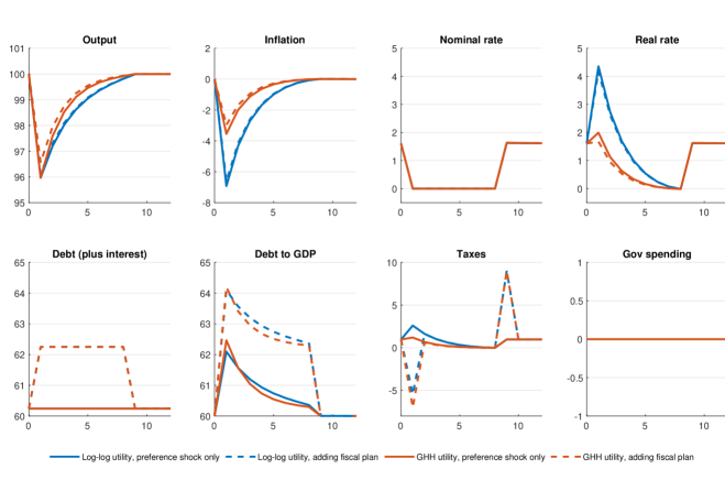
Figure 5: Impulse responses to a preference shock with and without fiscal intervention.
Notes: Inflation and interest rates are expressed in annualized percentage points. Taxes are expressed as percentage of quarterly output. Debt is expressed as percentage of annual output.

Table 5. Simulated debt multipliers for an expansion in debt
Panel a. Multipliers under log-log preferences
	Temporary change			Permanent change
	Normal times	ZLB		Normal times	ZLB
Impact
$q=0.9512$	$0.0006$	$0.0189$		$0.0000$	$0.0387$
$q=0.95$	$0.0006$	$0.0199$		$0.0000$	$0.0407$
$q=0.96$	$0.0004$	$0.0128$		$0.0000$	$0.0261$
$q=0.97$	$0.0002$	$0.0072$		$0.0000$	$0.0148$
$q=0.98$	$0.0001$	$0.0033$		$0.0000$	$0.0067$
$q=0.99$	$0.0000$	$0.0009$		$0.0000$	$0.0018$
Present value
$q=0.9512$	$0.0010$	$0.0073$		$0.0000$	$0.0131$
$q=0.95$	$0.0011$	$0.0076$		$0.0000$	$0.0138$
$q=0.96$	$0.0007$	$0.0049$		$0.0000$	$0.0088$
$q=0.97$	$0.0004$	$0.0028$		$0.0000$	$0.0050$
$q=0.98$	$0.0002$	$0.0013$		$0.0000$	$0.0023$
$q=0.99$	$0.0000$	$0.0003$		$0.0000$	$0.0006$
Panel b. Multipliers under GHH preferences
	Temporary change			Permanent change
	Normal times	ZLB		Normal times	ZLB
Impact
$q=0.9785$	$0.0004$	$0.0707$		$0.0000$	$0.1387$
$q=0.95$	$0.0022$	$0.3766$		$0.0006$	$0.7439$
$q=0.96$	$0.0013$	$0.2380$		$0.0003$	$0.4686$
$q=0.97$	$0.0007$	$0.1359$		$0.0001$	$0.2672$
$q=0.98$	$0.0003$	$0.0614$		$0.0000$	$0.1205$
$q=0.99$	$0.0001$	$0.0167$		$0.0000$	$0.0328$
Present value
$q=0.9785$	$0.0013$	$0.0230$		$0.0000$	$0.0401$
$q=0.95$	$0.0068$	$0.1257$		$0.0006$	$0.2216$
$q=0.96$	$0.0044$	$0.0785$		$0.0003$	$0.1378$
$q=0.97$	$0.0025$	$0.0444$		$0.0001$	$0.0777$
$q=0.98$	$0.0011$	$0.0200$		$0.0000$	$0.0348$
$q=0.99$	$0.0003$	$0.0054$		$0.0000$	$0.0094$

Notes: Impact multipliers are computed as the ratio between the impact variation of output (induced by the fiscal shock only) and the impact variation of debt. In the temporary debt plan, debt is raised in period 1 and brought back to the initial level in period 9, when the recession ends. In the permanent debt plan, debt is raised once and for all in period 1. Present value multipliers are computed using the formula in footnote 23, setting $k=8$.

The debt multipliers resulting from the simulations are shown in Table 5. To assess the overall effect of the fiscal plan, we consider both the impact multiplier and the present value multiplier, where the latter is computed as the present value of the variation in output during the recession period divided by the present value of the variation in debt. Under both types of preferences and both types of fiscal plans, debt multipliers are negligible in a mild recession scenario, but they are of one or two orders of magnitude larger when a severe recession hits the economy and monetary policy is constrained by the ZLB. In this case, the central bank does not adjust nominal rates upwards when the government implements the stimulus plan, as even lower rates would be required to contrast the adverse preference shock. As explained in Eggertsson (2011), at the ZLB the aggregate demand curve is actually upward sloping—rather than downward sloping as in standard theory—because the central bank does not offset inflationary pressures with interest rates hikes. In this case, a higher inflation means a lower real interest rate, implying higher demand and, in turn, larger fiscal multipliers.

The effectiveness of fiscal interventions depends on the reaction of monetary policy: when this reaction is muted, debt multipliers are more sizeable. But are they large enough to convince us that the debt level is a relevant policy instrument during a liquidity trap? Our simulations indicate that this can indeed be the case, but three elements are required. Two of them pertain to the structure of the model and are given by the size of the survival probability and the form of the utility function. When $q$ gets smaller, the model becomes increasingly less Ricardian and the wealth effects of debt play a more significant role, so that multipliers are magnified. Moreover, when households have GHH preferences rather than log-log preferences, the increase in consumption does not depress labor supply, and this again contributes to making multipliers bigger. The third element is instead related to the design of the fiscal plan. A permanent increase in debt produces a stronger response in output, as agents anticipate that the initial tax cut will not be reverted at the end of the recession. If we combine these three elements—i.e., set $q$ to 0.95, choose GHH preferences, and consider a permanent expansion in debt—we obtain a debt multiplier equal to 0.74 on impact, a figure that is not so distant from the estimates of the government spending multipliers reported by the recent literature. If we consider only a temporary expansion in debt, the associated impact multiplier reduces to 0.38, which may be considered as a small yet not irrelevant value.

Note that we assume that the fiscal stimulus only alleviates the fall in output caused by the preference shock, as the tax cut is too small to bring the economy back into the positive interest rates territory: the ZLB episode ends only when the preference shock eventually disappears, as shown in Figure 5.

Table 5 also implicitly illustrates the cost of a fiscal contraction engineered through the opposite policy, that is, through a temporary decrease in public debt caused by an initial tax hike followed by a cut. The main message is that fiscal consolidation through a temporary decrease in government debt may not be too costly in terms of output losses. However, this is true only as long as there are wealth effects on the labor supply (as in the case of log-log preferences) and the ZLB is not binding. This consideration emphasizes once again the perils of implementing a fiscal consolidation during a severe recession, when the central bank is unable to mitigate the negative consequences on output and prices. A fiscal restriction has an opposite effect on demand, and this effect will be amplified by the mechanism explained above. A restrictive fiscal intervention has deflationary effects, and when interest rates are constrained at the zero level, the central bank could not cut the interest rates to counteract deflation. Thus, the real interest rate will be higher leading to even lower demand.

5.1 Debt multipliers and the level of debt  

In the previous section we discussed the size of debt multipliers implied by our model when the stock of public debt amounts to 60% of GDP. A natural question is how previous findings change once we consider a different level of debt, and, in particular, once we increase the steady state debt-to-GDP ratio to match the values recently reached by most industrialized countries after the 2008 recession.

The analytic results of Sections 4.2 and 4.3 showed that the multipliers of the linearized version of the model directly depend on the steady state real interest rate, both in normal times and during a ZLB episode. In turn, the steady state real rate depends on the steady state debt-to-GDP ratio. Given our calibration strategy, Figure 2 also illustrates the relations (28) and (34). The implied increase in rates is pronounced: when the debt-to-GDP ratio passes from 60% to 200%, the annualized steady state real rate rises from 1.62% to 3.65%. As such, the level of debt is potentially a key variable for the size of debt multipliers.

To further examine the relation between the debt multiplier and the level of debt, we run another set of simulations in which we fix the size of the preference shock and we evaluate the effect of an expansion in debt for different levels of the initial debt-to-GDP ratio. Results are reported in Figure 6, where we show impulse responses of the economy after a temporary debt plan implemented at the ZLB, with log-log preferences. The preference shock is calibrated so that output contracts by 4% when the debt-to-GDP ratio is 60%. In this case the nominal rate remains at the ZLB for the entire duration of the recession. In the bottom-right panel of Figure 6, we show the ratio between the variation in debt and the steady state level of annual output, which is the same for all the cases considered. For a 60% debt-to-GDP ratio, the figure implies a debt multiplier of magnitude 0.0189 (as in Table 5), computed as the ratio between the impact increase of output (0.151%, in terms of quarterly output units) and the impact variation in debt (8%, again in quarterly terms).

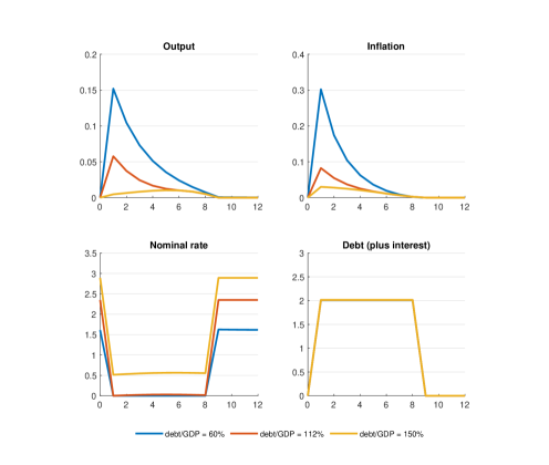
Figure 6: Impulse responses to a temporary increase in debt.
Notes: Impulse responses for output, inflation and debt-to-GDP represent the difference between the series generated with both the preference shock and the fiscal plan and the series generated with the preference shock only. The fiscal stimulus is given by a tax cut that raises the debt-to-GDP ratio by 2 percentage points in period 1, followed by a tax hike in period 9 that brings debt to its steady state level. All variables are in percentage points. The nominal interest rate and inflation are annualized. In the bottom-right panel, we show the ratio between the variation in debt and the steady state level of annual output.

For a debt-to-GDP ratio of 112%, the economy still falls into the ZLB on impact, but nominal rates can be lifted above zero already in second period. The intuition is that the steady state real rate increases with the level of steady state debt. It follows that the central bank starts from a higher nominal rate, for a given inflation target, and thus it has additional room to reduce rates and contrast the adverse preference shock. Being out from the ZLB, monetary policy is able to partially offset the positive demand shock represented by fiscal intervention, so that the responses of output and inflation are largely muted if compared to the 60% debt-to-GDP scenario. When debt is equal to 150% of GDP, the central bank can maintain interest rates above the zero limit and the expansionary effect of the fiscal stimulus plan is even weaker. The implied debt multiplier is negligible. The main takeaway here is that the steady state level of debt-to-GDP ratio could provide an alternative route to keep the economy away from the ZLB. Some papers in the literature (e.g., Blanchard et al., 2010) suggested to increase the inflation target to increase the steady state nominal rate (for a given steady state real rate) in order to provide monetary policy with more room for manoeuvre in case of a deflationary shock. This generated some debate in the literature (for a recent survey see Ascari and Sbordone, 2014). Here, we uncover an alternative route, based on the fact that in an OLG model (as well as in the data) the steady state real rate is an increasing function of the debt-to-GDP ratio. Hence, a rise in the debt-to-GDP ratio could provide monetary policy with more room for manoeuvre in case of a deflationary shock, because it increases the steady state nominal rate, through a rise in the steady state real rate (for a given steady state inflation target).

6 Conclusions

This paper analyzes the debt multiplier, that is, it addresses the consequences on economic activity of a temporary change in government debt in a simple OLG model, in which agents exhibit non-Ricardian behavior. Variations in lump-sum taxes fully reversed in the future generate wealth effects that influence the consumption and labor choices. One could consider the debt multiplier as a complement to the fiscal multipliers so far appeared in the literature, mainly featuring an ILRA framework. The debt multiplier would be the additional multiplier that one can get if any temporary fiscal policy measure would be financed through a pure temporary increase in public debt (i.e., a postponement of lump-sum taxes). We show that the debt multiplier is positive in an OLG framework. As for other fiscal multipliers analyzed in the literature, the debt multiplier depends critically on the stance of monetary policy and it is larger when interest rates are stuck at the zero bound and the subsequent adjustment in taxes is delayed until the recession has ended. Moreover, the debt multiplier increases with the level of debt-to-GDP ratio. Finally, we point out that, since the steady state real interest rate is increasing with the steady state level of debt-to-GDP ratio, a rise in the debt-to-GDP ratio could provide an alternative way to stay away from the ZLB.

References

- Adjemian et al. (2011) Adjemian, S., H. Bastani, F. Karamé, M. Juillard, J. Maih, F. Mihoubi, G. Perendia, J. Pfeifer, M. Ratto, and S. Villemot (2011): “Dynare: Reference Manual Version 4,” Dynare Working Papers 1, CEPREMAP.
- Ascari and Rankin (2007) Ascari, G. and N. Rankin (2007): “Perpetual youth and endogenous labor supply: A problem and a possible solution,” Journal of Macroeconomics, 29, 708–723.
- Ascari and Rankin (2013) ——— (2013): “The effectiveness of government debt for demand management: Sensitivity to monetary policy rules,” Journal of Economic Dynamics and Control, 37, 1544–1566.
- Ascari and Sbordone (2014) Ascari, G. and A. M. Sbordone (2014): “The Macroeconomics of Trend Inflation,” Journal of Economic Literature, 52, 679–739.
- Auerbach and Gorodnichenko (2012) Auerbach, A. J. and Y. Gorodnichenko (2012): “Measuring the Output Responses to Fiscal Policy,” American Economic Journal: Economic Policy, 4, 1 – 27.
- Auerbach and Gorodnichenko (2013) ——— (2013): “Fiscal Multipliers in Recession and Expansion,” in Fiscal Policy after the Financial Crisis, ed. by A. Alesina and F. Giavazzi, University of Chicago Press, chap. 2, 63–98.
- Bilbiie (2011) Bilbiie, F. O. (2011): “Nonseparable Preferences, Frisch Labor Supply, and the Consumption Multiplier of Government Spending: One Solution to a Fiscal Policy Puzzle,” Journal of Money, Credit and Banking, 43.
- Bilbiie et al. (2013) Bilbiie, F. O., T. Monacelli, and R. Perotti (2013): “Public Debt and Redistribution with Borrowing Constraints,” The Economic Journal, 123, F64 – F98.
- Blanchard et al. (2010) Blanchard, O., G. Dell’Ariccia, and P. Mauro (2010): “Rethinking macroeconomic policy,” Journal of Money, Credit and Banking, 42, 199–215.
- Blanchard (1985) Blanchard, O. J. (1985): “Debt, Deficits, and Finite Horizons,” Journal of Political Economy, 93, 223–247.
- Blanchard and Leigh (2013) Blanchard, O. J. and D. Leigh (2013): “Growth Forecast Errors and Fiscal Multipliers,” American Economic Review, 103, 117–20.
- Blanchard and Leigh (2014) ——— (2014): “Leraning about Fiscal Multipliers from Growth Forecast Errors,” IMF Economic Review, 62, 179–212.
- Caggiano et al. (2015) Caggiano, G., E. Castelnuovo, V. Colombo, and G. Nodari (2015): “Estimating Fiscal Multipliers: News From A Non-linear World,” The Economic Journal, 125, 746–776.
- Calvo (1983) Calvo, G. A. (1983): “Staggered prices in a utility-maximizing framework,” Journal of Monetary Economics, 12, 383–398.
- Castelnuovo and Nisticò (2010) Castelnuovo, E. and S. Nisticò (2010): “Stock market conditions and monetary policy in a DSGE model for the U.S.” Journal of Economic Dynamics and Control, 34, 1700 – 1731.
- Christiano et al. (2011) Christiano, L., M. Eichenbaum, and S. Rebelo (2011): “When Is the Government Spending Multiplier Large?” Journal of Political Economy, 119, 78–121.
- Devereux (2011) Devereux, M. B. (2011): “Fiscal Deficits, Debt, and Monetary Policy in a Liquidity Trap,” in Monetary Policy under Financial Turbulence, ed. by L. F. Céspedes, R. Chang, and D. Saravia, Central Bank of Chile, vol. 16 of Central Banking, Analysis, and Economic Policies Book Series, chap. 10, 369–410.
- Eggertsson (2011) Eggertsson, G. B. (2011): “What Fiscal Policy is Effective at Zero Interest Rates?” in NBER Macroeconomics Annual 2010, Volume 25, National Bureau of Economic Research, Inc, NBER Chapters, 59–112.
- Engen and Hubbard (2004) Engen, E. M. and R. G. Hubbard (2004): “Federal Government Debt and Interest Rates,” in NBER Macroeconomics Annual, National Bureau of Economic Research, Inc, vol. 19 of NBER Chapters, 83–160.
- Fazzari et al. (2015) Fazzari, S. M., J. Morley, and I. Panovska (2015): “State-dependent effects of fiscal policy,” Studies in Nonlinear Dynamics Econometrics, 19, 285–315.
- Gale and Orszag (2005) Gale, W. G. and P. R. Orszag (2005): “Deficits, Interest Rates, and the User Cost of Capital: A Reconsideration of the Effects of Tax Policy on Investment,” National Tax Journal, 58, 409–426.
- Giambattista and Pennings (2017) Giambattista, E. and S. Pennings (2017): “When is the government transfer multiplier large?” European Economic Review, 100, 525 – 543.
- Greenwood et al. (1988) Greenwood, J., Z. Hercowitz, and G. W. Huffman (1988): “Investment, Capacity Utilization, and the Real Business Cycle,” American Economic Review, 78, 402–417.
- Laubach (2009) Laubach, T. (2009): “New Evidence on the Interest Rate Effects of Budget Deficits and Debt,” Journal of the European Economic Association, 7, 858–885.
- Leeper et al. (2010) Leeper, E. M., M. Plante, and N. Traum (2010): “Dynamics of fiscal financing in the United States,” Journal of Econometrics, 156, 304 – 321.
- Leeper et al. (2017) Leeper, E. M., N. Traum, and T. B. Walker (2017): “Clearing Up the Fiscal Multiplier Morass,” American Economic Review, 107, 2409–54.
- Lindé and Trabandt (2018) Lindé, J. and M. Trabandt (2018): “Should we use linearized models to calculate fiscal multipliers?” Journal of Applied Econometrics, 33, 937–965.
- Mehrotra (2018) Mehrotra, N. R. (2018): “Fiscal Policy Stabilization: Purchases or Transfers?” International Journal of Central Banking, 14, 1 – 49.
- Monacelli and Perotti (2008) Monacelli, T. and R. Perotti (2008): “Fiscal Policy, Wealth Effects, and Markups,” NBER Working Papers 14584, National Bureau of Economic Research, Inc.
- Mountford and Uhlig (2009) Mountford, A. and H. Uhlig (2009): “What are the effects of fiscal policy shocks?” Journal of Applied Econometrics, 24, 960–992.
- Ramey (2011) Ramey, V. A. (2011): “Can Government Purchases Stimulate the Economy?” Journal of Economic Literature, 49, 673–85.
- Ramey (2019) ——— (2019): “Ten Years after the Financial Crisis: What Have We Learned from the Renaissance in Fiscal Research?” Journal of Economic Perspectives, 33, 89–114.
- Ramey and Zubairy (2018) Ramey, V. A. and S. Zubairy (2018): “Government Spending Multipliers in Good Times and in Bad: Evidence from U.S. Historical Data,” Journal of Political Economy, 126, 850–901.
- Sgherri and Bayoumi (2006) Sgherri, S. and T. Bayoumi (2006): “Mr. Ricardo’s Great Adventure; Estimating Fiscal Multipliers in a Truly Intertemporal Model,” IMF Working Papers 06/168, International Monetary Fund.
- Smets and Trabandt (2018) Smets, F. and M. Trabandt (2018): “Government Debt, the Zero Lower Bound and Monetary Policy,” Mimeo.
- Woodford (2011) Woodford, M. (2011): “Simple Analytics of the Government Expenditure Multiplier,” American Economic Journal: Macroeconomics, 3, 1–35.
- Zubairy (2014) Zubairy, S. (2014): “On Fiscal Multipliers: Estimates from a Medium-Scale DSGE Model,” International Economic Review, 55, 169–195.