Science Extraction from TESS Observations of Known Exoplanet Hosts

Abstract

The transit method of exoplanet discovery and characterization has enabled numerous breakthroughs in exoplanetary science. These include measurements of planetary radii, mass-radius relationships, stellar obliquities, bulk density constraints on interior models, and transmission spectroscopy as a means to study planetary atmospheres. The Transiting Exoplanet Survey Satellite (TESS) has added to the exoplanet inventory by observing a significant fraction of the celestial sphere, including many stars already known to host exoplanets. Here we describe the science extraction from TESS observations of known exoplanet hosts during the primary mission. These include transit detection of known exoplanets, discovery of additional exoplanets, detection of phase signatures and secondary eclipses, transit ephemeris refinement, and asteroseismology as a means to improve stellar and planetary parameters. We provide the statistics of TESS known host observations during Cycle 1 & 2, and present several examples of TESS photometry for known host stars observed with a long baseline. We outline the major discoveries from observations of known hosts during the primary mission. Finally, we describe the case for further observations of known exoplanet hosts during the TESS extended mission and the expected science yield.

1 Introduction

Discoveries of exoplanets have increased dramatically over the past two decades, largely due to the implementation of the transit method (Borucki & Summers, 1984; Hubbard et al., 2001). In particular, space-based photometry combined with large-scale survey strategies are able to overcome both the transit probability distribution and the observational window function that can impede ground-based approaches (Kane & von Braun, 2008; von Braun et al., 2009). Significant contributors to the space-based transit survey approaches have been the Convection, Rotation and planetary Transits (CoRoT) mission (Auvergne et al., 2009) and the Kepler mission (Borucki et al., 2010). In 2018, the Transiting Exoplanet Survey Satellite (TESS) was launched to begin its transit survey of the nearest and brightest stars (Ricker et al., 2015). The advantage of such bright stars is their suitability for follow-up observations that measure planetary masses (Fischer et al., 2016; Burt et al., 2018) and atmospheric compositions via transmission spectroscopy (Seager & Sasselov, 2000; Kempton et al., 2018). Each of the first two years of the TESS mission were devoted to observing the southern and northern ecliptic hemispheres, respectively, during which a vast discovery space was predicted (Sullivan et al., 2015; Barclay et al., 2018).

The survey design strategy of TESS has resulted in the observation of stars already known to host exoplanets that were discovered through a variety of methods. The continuous time series photometry of these stars may be used to achieve multiple science goals that have an over-arching theme of unprecedented characterization of these planetary systems. These science goals include the detection of transits for known planets (Dalba et al., 2019), the discovery of additional planets (Brakensiek & Ragozzine, 2016), the detection of phase variations and secondary eclipses (Mayorga et al., 2019), refinement of transit ephemerides (Dragomir et al., 2020), and asteroseismology of host stars (Campante et al., 2016). Each of these science goals have been realized to various degrees through the course of the TESS primary mission, providing significant insight into the physical properties of the known planets and the architectures of those systems.

In this paper, we provide a description of the science motivation behind TESS observations of known exoplanet host stars during the primary mission, along with statistics of these observations and a summary of the results. Note that “known hosts” in this work refers to stars that are known to host planets outside of TESS discoveries. In Section 2 we present the details for each of the science cases and quantify the advantage of returning to known exoplanet hosts. Section 3 provides the statistics of the known exoplanet host TESS observations, together with several examples of TESS photometry for hosts observed over multiple sectors. Section 4 summarizes the published science results regarding known exoplanet hosts from the TESS primary mission, and Section 5 discusses possible further science yield from continuing to observe known hosts during the extended mission. Section 6 provides concluding remarks and suggestions for additional science exploitation of known host observations and follow-up programs.

2 The Advantage of Observing Known Hosts

There are numerous science motivations for observing known exoplanet host stars. Here we discuss several of those motivations, including transit detection of known planets, discovery of new planets, phase signatures and secondary eclipses, transit ephemeris refinement, and asteroseismology.

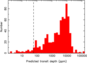
Figure 1: Histogram of predicted transit depths for all known RV planets. The vertical dashed line at 60 ppm represents the engineering requirement for the noise floor of the TESS photometric precision (actual noise floor is closer to 20 ppm).

2.1 Transit Detection of Known Exoplanets

At the current time, it remains unknown if many of the radial velocity (RV) detected exoplanets transit their host stars. Since these host stars are relatively bright, they provide numerous opportunities for detailed characterization of the systems, such as transmission spectroscopy, orbital dynamics, and potential targets for future imaging missions (Winn & Fabrycky, 2015; Kane et al., 2018; Batalha et al., 2019). The detection of transits for known planets has been discussed in detail (Kane, 2007; Kane et al., 2009; Hill et al., 2020), including the transit probabilities of such planets (Kane & von Braun, 2008; Stevens & Gaudi, 2013). A study of anticipated TESS observations of known exoplanet hosts was carried out by Dalba et al. (2019). Accounting for the transit probability, visibility of targets, and observing cadence, this study estimated that $11.7\pm 0.3$ known RV planets would exhibit transits during TESS primary mission observations, 3 of which would be new transit discoveries.

Shown in Figure 1 is a histogram of predicted transit depths for known RV planets that have not had a transit detected. The necessary data were extracted from the NASA Exoplanet Archive (Akeson et al., 2013) on 2020 May 5, and we retained all cases with the necessary planetary and stellar information. Numerous exoplanet mass-radius relationships have been derived (Kane & Gelino, 2012b; Weiss & Marcy, 2014; Chen & Kipping, 2017), and we adopt the methodology of Zeng et al. (2019), which uses a Monte Carlo approach with a planet formation motivated growth model, to estimate planetary radii from the minimum planetary masses. As a result, a total of 749 planets are included in the histogram. According to Ricker et al. (2015), the engineering requirement for the systematic noise floor of the photometric precision over one hour timescales was $\sim$60 ppm, shown in Figure 1 as a vertical dashed line. Of the 749 planets included, the predicted transit depths of 709 fall above this 60 ppm threshold. There are many other factors, such as additional noise sources (Feinstein et al., 2019), geometric transit probability (Kane & von Braun, 2008), and transit window functions (von Braun et al., 2009), that truncate the expected number of observed transits during TESS observations (Dalba et al., 2019). Fortunately, the in-flight reassessment of the photometric precision noise floor found the performance to be better than the engineering requirements. In most cases, the photometric precision of TESS is sufficient to detect transits of known RV planets should their inferior conjunction occur during the TESS observing windows.

2.2 Discovery of Additional Planets

One of the major reasons to continue monitoring known host stars is the prospect of detecting additional planets within those systems, regardless of the detection technique that was used to discover the known planets (Dietrich & Apai, 2020). Continued monitoring and discovery of additional planets is an essential pathway toward revealing the full diversity of planetary architectures (Winn & Fabrycky, 2015), including dynamical interactions (Kane & Raymond, 2014; Agnew et al., 2019) and coplanrity (Fang & Margot, 2012; Becker et al., 2017). For example, the WASP-47 system, initially detected as a single hot-Jupiter (Hellier et al., 2012), has been revealed as a complex multi-planet system and the focus of numerous follow-up efforts (Becker et al., 2015; Dai et al., 2015; Almenara et al., 2016; Sinukoff et al., 2017; Vanderburg et al., 2017; Weiss et al., 2017; Kane et al., 2020a). Although long-term photometric monitoring will only reveal those planets that happen to have orbital alignments favorable for transit detection, such planets typically fall within the demographic of short-period terrestrial planets that were below the detection threshold of previous surveys.

2.3 Phase Variations and Secondary Eclipses

In the era of precision photometry, particularly from space-based facilities, the detection of phase variations of exoplanets has become a powerful method to probe atmospheric properties (Faigler & Mazeh, 2011; Shporer, 2017). Phase variations caused by reflected light can provide insight into the scattering properties of an exoplanet’s atmosphere (Burrows et al., 2010; Kane & Gelino, 2010, 2011b; Madhusudhan & Burrows, 2012) and can disentangle multi-planet systems through sustained monitoring (Kane & Gelino, 2013; Gelino & Kane, 2014). These reflected light signatures complement the thermal structure and orbital information inferred from phase variations and secondary eclipses detected in the infrared (Harrington et al., 2006; Knutson et al., 2007; Kane & von Braun, 2009; Kane & Gelino, 2011a; Demory et al., 2016). Secondary eclipse observations enable the measurement of atmospheric temperatures that are critical in modeling exoplanet atmospheres and interiors (Line & Yung, 2013; von Paris et al., 2016; Fortney et al., 2019). Furthermore, the additional phase variation components of ellipsoidal variations and Doppler beaming can be used to distinguish between stellar and planetary companions to the host star (Drake, 2003; Kane & Gelino, 2012a). The TESS bandpass primarily spans optical wavelengths (Ricker et al., 2015), so the recovered phase signatures will be dominated by the reflected light component.

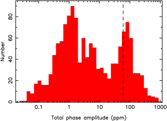
Figure 2: Top: histogram of the total phase amplitude for all of the planets described in Section 2.3. The vertical dashed line at 60 ppm represents the noise floor of the TESS photometric precision. Bottom: predicted phase amplitudes for KELT-1b, including reflected light (dashed), ellipsoidal (dotted), Doppler beaming (dot-dashed), and total (solid).

We used the stellar and exoplanet data from the NASA Exoplanet Archive, as described in Section 2.1, to calculate the reflected light, ellipsoidal variation, and Doppler beaming components for all known planets with the necessary information. A histogram of the combined amplitude for all three effects is shown in the top panel of Figure 2, including a total of 1384 planets. As for Figure 1, the vertical dashed line represents the systematic noise floor of the TESS photometric precision, of which 291 phase amplitudes lie above. For the purposes of the reflected light calculations, the geometric albedo for all planets was assumed to be 0.5 and we use the Keplerian orbital information where available. The bi-model shape in the distribution arises from a combination of exoplanet survey observational biases, and the gaps observed in both the period and mass/size of exoplanets (Matsakos & Königl, 2016; Mazeh et al., 2016; Fulton et al., 2017), for which the amplitudes of the various phase components are very sensitive. In other words, the distribution that peaks near 100 ppm is dominated by hot Jupiter planets. For example, the predicted phase amplitudes of KELT-1b, a $\sim$27 $M_{J}$ brown dwarf in a 1.22 day period orbit (Siverd et al., 2012), are represented in the bottom panel of Figure 2. The reflected light, ellipsoidal, and Doppler beaming components are shown as dashed, dotted, and dot-dashed lines respectively, and the total variations are shown as a solid line. Orbital phase zero corresponds to a planet location of superior conjunction, or ”full” reflection phase. In this extreme case, the combination of high mass and size, along with small star–planet separation, results in relatiely high ampltudes for all three components of the variations, placing it firmly within the right-hand part of the distribution shown in the top panel of Figure 2.

2.4 Transit Ephemeris Refinement

The atmospheric characterization community has the ambition to study hundreds of planets over the next decade in order to reveal the statistics of exoplanet atmospheres. This will be largely achieved with a combination of the James Webb Space Telescope (JWST) and dedicated missions, such as the Atmospheric Remote-sensing Infrared Exoplanet Large-survey (ARIEL) mission (Puig et al., 2016; Kempton et al., 2018). A significant issue facing the observational planning for atmospheric signatures of known transiting planets is the reduced quality of their transit ephemerides with time (Kane et al., 2009). The errors are dominated by uncertainties in the periods, which could be significantly reduced by observing just a handful of transits at the TESS epoch (Dragomir et al., 2020; Zellem et al., 2020). Figure 3 shows a histogram of the 95% confidence window (i.e., $\pm 2\sigma$) for transit times of 1457 well-studied transiting planets listed in the Transiting Extrasolar Planets Catalogue (Southworth, 2011). The windows were calculated for a representative date (January 1, 2025) when JWST is expected to be in full operation. More than half of the known planets will have windows greater than 2 hours, which means that observations of their transits or eclipses would require significant additional observing time to have a guaranteed observations of a full transit event. Improvement of transit ephemerides will be achieved via the use of various follow-up facilities, including CHaracterizing ExOPlanets Satellite (CHEOPS) observations of TESS targets (Broeg et al., 2014; Cooke et al., 2020).

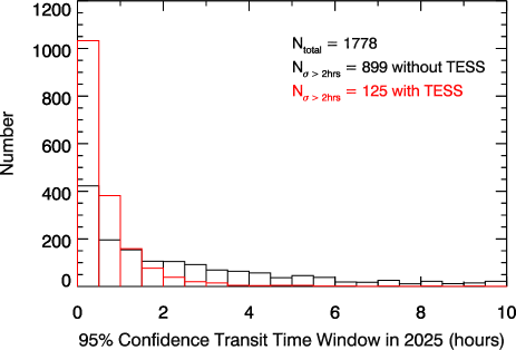
Figure 3: Histograms of the 95% confidence window for transit times of 1457 known transiting exoplanets, projected forward to January 1, 2025. The red and the black histograms are with and without TESS observations respectively.

Some of the most exciting science from Kepler came from systems of multiple transiting planets, particularly those where planet-planet interactions revealed by Transit Timing Variations (TTVs) provided an important source of mass measurements and constraints (e.g., Steffen et al., 2013; Hadden & Lithwick, 2014). Such observations of TTVs are also true for TESS but to a more limited extent (Goldberg et al., 2019; Hadden et al., 2019). Kane et al. (2019) investigated the degradation of TTV signals when switching from Kepler’s 4-year duration to the 6–12 month duration of TESS. Using a basic scaling estimate, they find that roughly tens of TESS planets will show TTVs, although only some of these will lead to useful mass constraints.

2.5 Asteroseismology

Asteroseismology is one of the most successful methods to precisely infer radii, masses, and ages of exoplanets through the characterization of their host stars (for recent reviews, see Huber, 2018; Lundkvist et al., 2018). We predicted the asteroseismic yield of known host stars in Cycles 1 and 2 by employing a statistical test (Chaplin et al., 2011; Campante et al., 2016; Schofield et al., 2019) that estimates the detectability of convection-driven, solar-like oscillations in TESS photometry of any given target. The expectation is that solar-like oscillations are detectable in nearly 100 solar-type (i.e., low-mass, main-sequence stars and cool subgiants) and red-giant known hosts, virtually all of which are RV systems (see Figure 4). Moreover, about half of such hosts are evolved stars, i.e., having $\log g<3.85$. The corresponding planet sample is mostly comprised of long-period gas giants, with a smaller fraction of hot Jupiters and warm super-Earths/Neptunes. To assess if asteroseismology can further constrain stellar and planetary properties, we estimated the precision with which fundamental stellar properties can be obtained for stars in the asteroseismic sample. We used the Bayesian code PARAM (da Silva et al., 2006; Rodrigues et al., 2014, 2017) to this end, a grid-based approach whereby observables are matched to well-sampled grids of stellar evolutionary models. Two different sets of observables were considered, one containing only spectroscopic data and a parallax-based luminosity (this allows reproducing the typical precision levels currently found in the literature), the other containing additional constraints from asteroseismology (namely, the predicted large frequency separation, $\Delta\nu$, and the predicted frequency of maximum oscillation amplitude, $\nu_{\rm max}$, both with uncertainties as expected for TESS). We found that by including asteroseismic constraints one can significantly improve (by a factor of 2–5) the precision of stellar properties when compared to estimates stemming from a combination of spectroscopy and astrometry alone (1.9 vs 3.4% in radius, 4.6 vs 6.7% in mass, 15 vs 30% in age, and 3.4 vs 15% in mean density). This asteroseismic sample will thus provide us with a benchmark ensemble of planets with precisely inferred radii, masses, and ages.

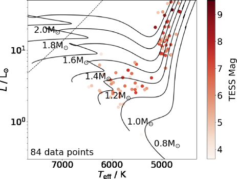
Figure 4: Predicted yield of known host stars in Cycles 1 and 2 having detectable solar-like oscillations. Solar-calibrated evolutionary tracks span the mass range 0.8–2.0 $M_{\odot}$. The slanting dashed line represents the red edge of the $\delta$ Scuti instability strip. Evolved stars (i.e., with $\log g<3.85$) make up about half of the yield.

3 Known Host Coverage

The nominal plan for TESS observations during the primary mission was to result in $\sim$85% sky coverage with a minimum observing baseline of $\sim$27 days (Ricker et al., 2015). Year 1 (Cycle 1) and year 2 (Cycle 2) of the mission were directed at the southern and northern ecliptic hemispheres, respectively. During Cycle 1, modifications were made to the location of the Cycle 2 sectors that shifted them north along a line of ecliptic longitude in order to minimize scattered light effects.

For our analysis of the TESS coverage of known exoplanet hosts during the primary mission, we include data from the NASA Exoplanet Archive (Akeson et al., 2013) from 2020 May 5, matching the sample described in Section 2.1 and Section 2.3. From these data, we exclude those exoplanet hosts whose planets were detected by TESS (45) and host stars without $V$ magnitude information (202). These restrictions reduce the planet sample from 4152 to 3912. For each host star, we determined the sectors during which they were observed by TESS using the proposal tools provided by the TESS Science Support Center.

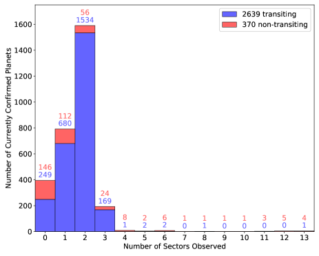
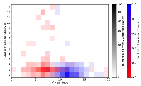
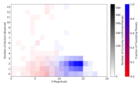
Figure 5: TESS coverage of the known exoplanets during the primary mission. The top-left and top-right panels show histograms of the number of sectors during which transiting (blue) and non-transiting (red) planets were covered during Cycle 1 and Cycle 2, respectively. The bottom-left and bottom-right panels show intensity maps of the known exoplanet coverage as a function of the host star $V$ magnitude during Cycle 1 and Cycle 2, respectively.

Shown in Figure 5 are plots that represent the TESS coverage of the known exoplanet hosts during the primary mission. The two left-hand panels in Figure 5 refer to Cycle 1 and the two right-hand panels refer to Cycle 2. The top two panels are histograms of the total number of sectors during that cycle for which exoplanets were covered by TESS observations, with transiting planets being shown in blue and planets not known to transit shown in red. The numbers above each bin indicate the number of planets represented by the transiting and non-transiting categories for that bin. Although the number of exoplanets covered during Cycle 1 are fairly evenly split between the transiting and non-transiting categories, the exoplanet sample in Cycle 2 was dominated by the observations of the Kepler field, most of which are too faint for TESS data to be profitable. We estimate the fraction of known exoplanet hosts covered by the TESS primary mission by removing those exoplanets with zero sector coverage (see bin 0 of the Figure 5 histograms) from the total number of exoplanets in our sample (3912). This results in a fractional exoplanet host coverage of $\sim$81.5%.

The bottom two panels of Figure 5 present the same data as for the top two panels, but in the form of intensity maps as a function of both sectors observed and the $V$ magnitude of the host stars. The shading and color of the bins relate to the number of planets in that bin and the relative fractions of transiting planets. These bottom two plots of Figure 5 emphasize the bimodal distribution of host star $V$ magnitudes between RV and transit surveys, resulting from the need of transit surveys for large stellar samples to overcome the geometric transit probability, thus including many more fainter stars than brighter stars (Kane et al., 2009). As for the top-right panel, the Kepler sample dominates the data shown in the bottom-right panel, causing an apparent lack of contrast in the intensity map.

Figure 5 indicates that a handful of known hosts were observed almost continuously during a given cycle of TESS observations. For example, consider the HD 40307 system, which was observed for 12 of the 13 sectors of Cycle 1. The system is known to contain at least 5 planets that are a mixture of super-Earths and mini-Neptunes discovered using the RV technique (Mayor et al., 2009; Tuomi et al., 2013; Díaz et al., 2016). Currently, none of the planets are known to transit the host star, a K2.5 dwarf (Tuomi et al., 2013). To calculate the transit probabilities and predicted transit depths, we combined the minimum planet masses of Tuomi et al. (2013) with the mass-radius relationship of Chen & Kipping (2017) to estimate radii of 1.8, 2.5, 3.0, 2.1, and 2.6 $R_{\oplus}$ for the b, c, d, f, and g planets, respectively. We further adopted the stellar radius estimate of $R_{\star}=0.7083$ $R_{\odot}$ provided by Valenti & Fischer (2005). These result in transit probabilities of 11.2%, 6.5%, 4.0%, 2.1%, and 0.9% for the b, c, d, f, and g planets, respectively. Note that these probabilities are calculated independently of each other and do not take into account coplanarity of the system. The calculated predicted transit depths are 215, 415, 598, 293, and 449 ppm for the b, c, d, f, and g planets, respectively.

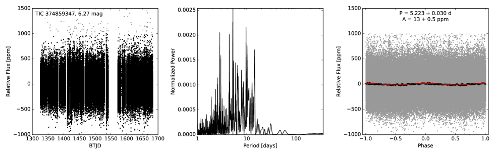
Figure 6: TESS observations of the known exoplanet host HD 40307. Left: light curve from 12 sectors of TESS observations during Cycle 1. Middle: a Lomb-Scargle periodogram calculated from the TESS photometry shown in the left panel. Right: photometry folded on the most significant period detected from the photometric variability analysis (5.223 days).

Shown in Figure 6 are the TESS photometry for HD 40307, with a 1$\sigma$ scatter of 203 ppm, and the results of a variability analysis of the data. The dates shown in the left panel are expressed in Barycentric TESS Julian Day (BTJD), where BTJD = BJD $-$ 2457000. We used the Presearch Data Conditioning (PDC) photometry, processed by the Science Processing Operations Center (SPOC) pipeline (Smith et al., 2012; Stumpe et al., 2012, 2014; Jenkins et al., 2016, 2020), and we extracted the data using the Lightkurve tool (Lightkurve Collaboration et al., 2018). The precision of the data is sufficient to rule out the previously calculated transits depths for all 5 planets. Even though the star was not observed during Sector 9, the longest period planet ($\sim$197 days) is sufficiently covered during Sectors 1–8 that the predicted 449 ppm for that planet can also be excluded from the data. An alternative explanation is that the planets do transit but their bulk densities are significantly higher than that predicted from typical mass-radius relationships. Examples such as the case of HD 40307 demonstrate the power of TESS to systematically achieve dispositive null detections of transits that are exceptionally difficult to achieve from ground-based observations (Wang et al., 2012).

4 Science From the Primary Mission

Observations of known exoplanet hosts during the TESS primary mission have realized many of the goals described in Section 2. Here we outline the major discoveries that have occurred in each of the Section 2 categories.

Transits of known planets (Section 2.1). A total of three known RV planets were discovered to transit from TESS observations during the primary mission. These include HD 118203b, a Jovian planet in a 6.13 day orbit (Pepper et al., 2020), and HD 136352 b and c, a super-Earth and mini-Neptune in 11.6 day and 27.6 day orbits, respectively (Kane et al., 2020b). The number of RV planets found to transit during the primary mission is aligned with the predictions of Dalba et al. (2019), which predicted three such discoveries.

New planets in known systems (Section 2.2). An early science result from TESS observations was the detection of an additional inner transiting planet in the Pi Mensae system (Huang et al., 2018). The combination of a Jovian planet in an eccentric 5.7 year period orbit with a mini-Neptune in a 6.27 day period orbit makes the system of dynamical interest (De Rosa et al., 2020; Xuan & Wyatt, 2020). Similarly, the long-period ($\sim$1600 days) Jovian planet in the HD 86226 system was found by Teske et al. (2020) to host a transiting mini-Neptune planet in a 3.98 day orbit.

Phase variations (Section 2.3). Numerous known transiting planets have been the subject of phase variation studies to place important constraints on their atmospheric properties. These include WASP-18b (Shporer et al., 2019), WASP-19b (Wong et al., 2020c), WASP-121b (Daylan et al., 2019), KELT-1b (Beatty et al., 2020), and KELT-9b (Wong et al., 2020a). Note that KELT-9b also exhibited an asymmetric transit in TESS photometry that was caused by rapid stellar rotation combined with a spin-orbit misalignment (Ahlers et al., 2020). A systematic study of phase curves detected for known transiting planets during Cycle 1 was carried out by Wong et al. (2020b).

Transit ephemeris refinement (Section 2.4). As described earlier, the refinement of transit ephemerides is a crucial component for enabling valuable follow-up observations, particularly those that involve atmospheric characterization (Kempton et al., 2018). A concerted effort has been undertaken by various teams to combine TESS data with ground-based observations (Yao et al., 2019; Cortés-Zuleta et al., 2020; Edwards et al., 2020) and K2 data (Ikwut-Ukwa et al., 2020) to improve the orbital properties of known transiting planets. Additionally, unexpected variations in the transit times of WASP-4b were detected by Bouma et al. (2019) and confirmed by Southworth et al. (2019), and were later explained by acceleration effects of the WASP-4 system (Bouma et al., 2020).

Stellar characterization through asteroseismology (Section 2.5). Several known exoplanet hosts have benefited from the TESS precision photometry during the primary mission, particularly those that have evolved past the main sequence. Campante et al. (2019) reported the detection of solar-like oscillations in the light curves of the red-giant exoplanet hosts HD 212771 and HD 203949. A further detection of solar-like oscillations was reported by Jiang et al. (2020) for the giant host star HD 222076, greatly improving the determined mass, radius, and age of the star. Nielsen et al. (2020) used TESS asteroseismology to firmly place the well-studied host $\lambda^{2}$ Fornacis at the early stage of its subgiant evolutionary phase.

5 Extended Mission Science Yield

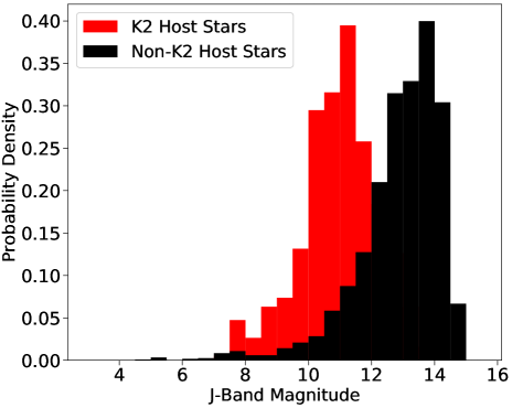
Figure 7: Histograms of host star $J$ magnitudes for exoplanets discovered via the transit method. Shown in red are those discovered with K2, and shown in black are those from all other transit surveys.

TESS has now moved in to the extended mission, from which further observations of known exoplanet host stars will result. For transits of known RV exoplanets, Dalba et al. (2019) predict that TESS will reveal one such planet be transiting for each year of the extended mission during which it returns to one of the hemispheres observed during the primary mission. As described in Section 2.1, the RV host stars are generally brighter than those of transit surveys, and so are valuable targets for follow-up observations. Likewise, extending the observations baseline for known systems, both transiting and non-transiting, will undoubtedly reveal further planets in those systems, adding to our statistical knowledge of planetary architectures. For the phase variations science, the advantage of returning to previously observed fields is to build signal-to-noise for small planet phase signatures that may have had an initial tenuous detection. The probability of detecting solar-like oscillations for a given star depends sensitively on the length of the observations (Chaplin et al., 2011; Campante et al., 2016; Schofield et al., 2019). As the baseline increases, so will the relative statistical fluctuations in the underlying background power in the Fourier spectrum decrease in magnitude. Consequently, further TESS observations of known hosts (even when the data are not contiguous) will allow the confirmation of previous tentative detections of oscillations as well as providing new detections.

Cycle 3 for TESS observations are returning to the southern ecliptic hemisphere, complementing the prior observations of the same stars during Cycle 1. Beyond Cycle 3, it is expected that TESS observations will turn to the ecliptic, observing stars not previously measured during the mission. Furthermore, the ecliptic observations will be carried out with the spacecraft rotated by 90$\arcdeg$ relative to the nominal pointing configuration. Such an observing strategy will cause a partial overlap of the camera fields with previously observed sectors in the northern and southern ecliptic, and significant overlap of with other ecliptic fields. This overlap of the ecliptic fields will result in a longer time baseline of observations relative to the $\sim$27 day duration for most of the camera pointings during the primary mission, allowing a much greater sensitivity to longer period planets and a higher science yield for many of the known host science cases described in this work. Another factor in favor of ecliptic observations are the relative brightness of the K2 mission host stars (whose transit discovery fields were largely centered along the ecliptic) and the subsequent potential for science return. Figure 7 shows histograms of the host star $J$ magnitude for planets that were discovered using the transit method. The histograms are for those cases discovered by K2 and those discovered via all other transit surveys (once again, excluding TESS). There is a clear bi-modality in the overall host star brightness distribution in which the K2 host stars are preferentially brighter. One effect of this brightness distribution is that K2 discoveries are more likely to result in successful atmospheric characterization studies (Kosiarek et al., 2019). To demonstrate this proposition, we used the Transmission Spectroscopy Metric (TSM) devised by Kempton et al. (2018), and recently applied to TESS exoplanet candidates (Ostberg & Kane, 2019). We calculated the TSM for all exoplanets with available data for the K2 and non-K2 groups represented in Figure 7. Note that faint host stars are less likely to have mass measurements for their planets (a required component of the TSM calculation), so in those cases we estimated the planet mass using the methodology of Chen & Kipping (2017). These TSM calculations revealed a mean value of 25.2 for the K2 population and 8.7 for the non-K2 population. Thus, TESS observations of the K2 host stars along the ecliptic would provide enormous benefits for the transit ephmeris refinement described in Section 2.4 in preparation for potential follow-up observations.

6 Conclusions

The TESS mission has completed a highly successful survey of the sky during the first two years. Although the discovery of previously unknown planetary systems is the primary science goal of the mission, TESS has provided serendipitous insights into previously known systems, aiding toward the characterization of some of the brightest and well-known host stars. As we have demonstrated here, $\sim$81.5% of known exoplanet hosts were observed during the primary mission, of which most of those outside the Kepler field were observed for a single sector. Regardless, the science yield for these targets was extensive, covering a broad range of topics.

The significant discoveries include transit detection of known RV planets orbiting nearby and bright host stars, such as the naked-eye star HD 136352, and additional transiting planets in known exosystems. The combination of precise photometry with the relatively bright exoplanet hosts of known transiting planets has enabled substantial progress to be made in the detection of phase variations, providing further constraints on the atmospheric properties for these planets. Observations of these known transiting systems has also greatly improved the precision of their measured orbital parameters, which is a critical factor in scheduled follow-up observations with large competitive facilities. Finally, the observation of evolved hosts by TESS has made it possible to greatly improve the properties of these stars, including mass, radius, and age, and thus better understand the planets that orbit them.

Beyond the primary mission, it is expected that further TESS observations of known exoplanet hosts will continue to yield exciting new results as the baseline of observations is increased and new fields along the ecliptic are covered. In particular, the extended baseline will likely reveal further transits of known and unknown planets for stars already known to harbor planets. As we have shown, these systems have preferentially bright host stars and will form a major contribution to the target selection for atmospheric characterization observations. Thus, an important component of the TESS legacy will be to establish the cornerstone systems whose history and future of observations place them amongst our best understood examples of planetary systems outside of the solar system.

References

- Agnew et al. (2019) Agnew, M. T., Maddison, S. T., Horner, J., & Kane, S. R. 2019, MNRAS, 485, 4703
- Ahlers et al. (2020) Ahlers, J. P., Johnson, M. C., Stassun, K. G., et al. 2020, AJ, 160, 4
- Akeson et al. (2013) Akeson, R. L., Chen, X., Ciardi, D., et al. 2013, PASP, 125, 989
- Almenara et al. (2016) Almenara, J. M., Díaz, R. F., Bonfils, X., & Udry, S. 2016, A&A, 595, L5
- Auvergne et al. (2009) Auvergne, M., Bodin, P., Boisnard, L., et al. 2009, A&A, 506, 411
- Barclay et al. (2018) Barclay, T., Pepper, J., & Quintana, E. V. 2018, ApJS, 239, 2
- Batalha et al. (2019) Batalha, N. E., Lewis, T., Fortney, J. J., et al. 2019, ApJ, 885, L25
- Beatty et al. (2020) Beatty, T. G., Wong, I., Fetherolf, T., et al. 2020, arXiv e-prints, arXiv:2006.10292
- Becker et al. (2017) Becker, J. C., Vanderburg, A., Adams, F. C., Khain, T., & Bryan, M. 2017, AJ, 154, 230
- Becker et al. (2015) Becker, J. C., Vanderburg, A., Adams, F. C., Rappaport, S. A., & Schwengeler, H. M. 2015, ApJ, 812, L18
- Borucki & Summers (1984) Borucki, W. J., & Summers, A. L. 1984, Icarus, 58, 121
- Borucki et al. (2010) Borucki, W. J., Koch, D., Basri, G., et al. 2010, Science, 327, 977
- Bouma et al. (2020) Bouma, L. G., Winn, J. N., Howard, A. W., et al. 2020, ApJ, 893, L29
- Bouma et al. (2019) Bouma, L. G., Winn, J. N., Baxter, C., et al. 2019, AJ, 157, 217
- Brakensiek & Ragozzine (2016) Brakensiek, J., & Ragozzine, D. 2016, ApJ, 821, 47
- Broeg et al. (2014) Broeg, C., Benz, W., Thomas, N., & Cheops Team. 2014, Contributions of the Astronomical Observatory Skalnate Pleso, 43, 498
- Burrows et al. (2010) Burrows, A., Rauscher, E., Spiegel, D. S., & Menou, K. 2010, ApJ, 719, 341
- Burt et al. (2018) Burt, J., Holden, B., Wolfgang, A., & Bouma, L. G. 2018, AJ, 156, 255
- Campante et al. (2016) Campante, T. L., Schofield, M., Kuszlewicz, J. S., et al. 2016, ApJ, 830, 138
- Campante et al. (2019) Campante, T. L., Corsaro, E., Lund, M. N., et al. 2019, ApJ, 885, 31
- Chaplin et al. (2011) Chaplin, W. J., Kjeldsen, H., Bedding, T. R., et al. 2011, ApJ, 732, 54
- Chen & Kipping (2017) Chen, J., & Kipping, D. 2017, ApJ, 834, 17
- Cooke et al. (2020) Cooke, B. F., Pollacco, D., Lendl, M., Kuntzer, T., & Fortier, A. 2020, MNRAS, 494, 736
- Cortés-Zuleta et al. (2020) Cortés-Zuleta, P., Rojo, P., Wang, S., et al. 2020, A&A, 636, A98
- da Silva et al. (2006) da Silva, L., Girardi, L., Pasquini, L., et al. 2006, A&A, 458, 609
- Dai et al. (2015) Dai, F., Winn, J. N., Arriagada, P., et al. 2015, ApJ, 813, L9
- Dalba et al. (2019) Dalba, P. A., Kane, S. R., Barclay, T., et al. 2019, PASP, 131, 034401
- Daylan et al. (2019) Daylan, T., Günther, M. N., Mikal-Evans, T., et al. 2019, arXiv e-prints, arXiv:1909.03000
- De Rosa et al. (2020) De Rosa, R. J., Dawson, R., & Nielsen, E. L. 2020, A&A, 640, A73
- Demory et al. (2016) Demory, B.-O., Gillon, M., de Wit, J., et al. 2016, Nature, 532, 207
- Díaz et al. (2016) Díaz, R. F., Ségransan, D., Udry, S., et al. 2016, A&A, 585, A134
- Dietrich & Apai (2020) Dietrich, J., & Apai, D. 2020, AJ, 160, 107
- Dragomir et al. (2020) Dragomir, D., Harris, M., Pepper, J., et al. 2020, AJ, 159, 219
- Drake (2003) Drake, A. J. 2003, ApJ, 589, 1020
- Edwards et al. (2020) Edwards, B., Changeat, Q., Yip, K. H., et al. 2020, MNRAS, arXiv:2005.01684
- Faigler & Mazeh (2011) Faigler, S., & Mazeh, T. 2011, MNRAS, 415, 3921
- Fang & Margot (2012) Fang, J., & Margot, J.-L. 2012, ApJ, 761, 92
- Feinstein et al. (2019) Feinstein, A. D., Montet, B. T., Foreman-Mackey, D., et al. 2019, PASP, 131, 094502
- Fischer et al. (2016) Fischer, D. A., Anglada-Escude, G., Arriagada, P., et al. 2016, PASP, 128, 066001
- Fortney et al. (2019) Fortney, J. J., Lupu, R. E., Morley, C. V., Freedman, R. S., & Hood, C. 2019, ApJ, 880, L16
- Fulton et al. (2017) Fulton, B. J., Petigura, E. A., Howard, A. W., et al. 2017, AJ, 154, 109
- Gelino & Kane (2014) Gelino, D. M., & Kane, S. R. 2014, ApJ, 787, 105
- Goldberg et al. (2019) Goldberg, M., Hadden, S., Payne, M. J., & Holman, M. J. 2019, AJ, 157, 142
- Hadden et al. (2019) Hadden, S., Barclay, T., Payne, M. J., & Holman, M. J. 2019, AJ, 158, 146
- Hadden & Lithwick (2014) Hadden, S., & Lithwick, Y. 2014, ApJ, 787, 80
- Harrington et al. (2006) Harrington, J., Hansen, B. M., Luszcz, S. H., et al. 2006, Science, 314, 623
- Hellier et al. (2012) Hellier, C., Anderson, D. R., Collier Cameron, A., et al. 2012, MNRAS, 426, 739
- Hill et al. (2020) Hill, M. L., Močnik, T., Kane, S. R., et al. 2020, AJ, 159, 197
- Huang et al. (2018) Huang, C. X., Burt, J., Vanderburg, A., et al. 2018, ApJ, 868, L39
- Hubbard et al. (2001) Hubbard, W. B., Fortney, J. J., Lunine, J. I., et al. 2001, ApJ, 560, 413
- Huber (2018) Huber, D. 2018, in Asteroseismology and Exoplanets: Listening to the Stars and Searching for New Worlds, ed. T. L. Campante, N. C. Santos, & M. J. P. F. G. Monteiro, Vol. 49, 119
- Ikwut-Ukwa et al. (2020) Ikwut-Ukwa, M., Rodriguez, J. E., Bieryla, A., et al. 2020, arXiv e-prints, arXiv:2007.00678
- Jenkins et al. (2020) Jenkins, J. M., Tenenbaum, P., Seader, S., et al. 2020, Kepler Data Processing Handbook: Transiting Planet Search, Kepler Data Processing Handbook (KSCI-19081-003),
- Jenkins et al. (2016) Jenkins, J. M., Twicken, J. D., McCauliff, S., et al. 2016, in Proc. SPIE, Vol. 9913, Software and Cyberinfrastructure for Astronomy IV, 99133E
- Jiang et al. (2020) Jiang, C., Bedding, T. R., Stassun, K. G., et al. 2020, ApJ, 896, 65
- Kane et al. (2019) Kane, M., Ragozzine, D., Flowers, X., et al. 2019, AJ, 157, 171
- Kane (2007) Kane, S. R. 2007, MNRAS, 380, 1488
- Kane et al. (2020a) Kane, S. R., Fetherolf, T., & Hill, M. L. 2020a, AJ, 159, 176
- Kane & Gelino (2010) Kane, S. R., & Gelino, D. M. 2010, ApJ, 724, 818
- Kane & Gelino (2011a) —. 2011a, ApJ, 741, 52
- Kane & Gelino (2011b) —. 2011b, ApJ, 729, 74
- Kane & Gelino (2012a) —. 2012a, MNRAS, 424, 779
- Kane & Gelino (2012b) —. 2012b, PASP, 124, 323
- Kane & Gelino (2013) —. 2013, ApJ, 762, 129
- Kane et al. (2009) Kane, S. R., Mahadevan, S., von Braun, K., Laughlin, G., & Ciardi, D. R. 2009, PASP, 121, 1386
- Kane et al. (2018) Kane, S. R., Meshkat, T., & Turnbull, M. C. 2018, AJ, 156, 267
- Kane & Raymond (2014) Kane, S. R., & Raymond, S. N. 2014, ApJ, 784, 104
- Kane & von Braun (2008) Kane, S. R., & von Braun, K. 2008, ApJ, 689, 492
- Kane & von Braun (2009) —. 2009, PASP, 121, 1096
- Kane et al. (2020b) Kane, S. R., Yalçınkaya, S., Osborn, H. P., et al. 2020b, AJ, 160, 129
- Kempton et al. (2018) Kempton, E. M. R., Bean, J. L., Louie, D. R., et al. 2018, PASP, 130, 114401
- Knutson et al. (2007) Knutson, H. A., Charbonneau, D., Allen, L. E., et al. 2007, Nature, 447, 183
- Kosiarek et al. (2019) Kosiarek, M. R., Crossfield, I. J. M., Hardegree-Ullman, K. K., et al. 2019, AJ, 157, 97
- Lightkurve Collaboration et al. (2018) Lightkurve Collaboration, Cardoso, J. V. d. M. a., Hedges, C., et al. 2018, Lightkurve: Kepler and TESS time series analysis in Python, , ascl:1812.013
- Line & Yung (2013) Line, M. R., & Yung, Y. L. 2013, ApJ, 779, 3
- Lundkvist et al. (2018) Lundkvist, M. S., Huber, D., Aguirre, V. S., & Chaplin, W. J. 2018, Characterizing Host Stars Using Asteroseismology (), 177
- Madhusudhan & Burrows (2012) Madhusudhan, N., & Burrows, A. 2012, ApJ, 747, 25
- Matsakos & Königl (2016) Matsakos, T., & Königl, A. 2016, ApJ, 820, L8
- Mayor et al. (2009) Mayor, M., Udry, S., Lovis, C., et al. 2009, A&A, 493, 639
- Mayorga et al. (2019) Mayorga, L. C., Batalha, N. E., Lewis, N. K., & Marley, M. S. 2019, AJ, 158, 66
- Mazeh et al. (2016) Mazeh, T., Holczer, T., & Faigler, S. 2016, A&A, 589, A75
- Nielsen et al. (2020) Nielsen, M. B., Ball, W. H., Standing, M. R., et al. 2020, A&A, 641, A25
- Ostberg & Kane (2019) Ostberg, C., & Kane, S. R. 2019, AJ, 158, 195
- Pepper et al. (2020) Pepper, J., Kane, S. R., Rodriguez, J. E., et al. 2020, AJ, 159, 243
- Puig et al. (2016) Puig, L., Pilbratt, G. L., Heske, A., Escudero Sanz, I., & Crouzet, P. E. 2016, in Society of Photo-Optical Instrumentation Engineers (SPIE) Conference Series, Vol. 9904, Space Telescopes and Instrumentation 2016: Optical, Infrared, and Millimeter Wave, 99041W
- Ricker et al. (2015) Ricker, G. R., Winn, J. N., Vanderspek, R., et al. 2015, Journal of Astronomical Telescopes, Instruments, and Systems, 1, 014003
- Rodrigues et al. (2014) Rodrigues, T. S., Girardi, L., Miglio, A., et al. 2014, MNRAS, 445, 2758
- Rodrigues et al. (2017) Rodrigues, T. S., Bossini, D., Miglio, A., et al. 2017, MNRAS, 467, 1433
- Schofield et al. (2019) Schofield, M., Chaplin, W. J., Huber, D., et al. 2019, ApJS, 241, 12
- Seager & Sasselov (2000) Seager, S., & Sasselov, D. D. 2000, ApJ, 537, 916
- Shporer (2017) Shporer, A. 2017, PASP, 129, 072001
- Shporer et al. (2019) Shporer, A., Wong, I., Huang, C. X., et al. 2019, AJ, 157, 178
- Sinukoff et al. (2017) Sinukoff, E., Howard, A. W., Petigura, E. A., et al. 2017, AJ, 153, 70
- Siverd et al. (2012) Siverd, R. J., Beatty, T. G., Pepper, J., et al. 2012, ApJ, 761, 123
- Smith et al. (2012) Smith, J. C., Stumpe, M. C., Van Cleve, J. E., et al. 2012, PASP, 124, 1000
- Southworth (2011) Southworth, J. 2011, MNRAS, 417, 2166
- Southworth et al. (2019) Southworth, J., Dominik, M., Jørgensen, U. G., et al. 2019, MNRAS, 490, 4230
- Steffen et al. (2013) Steffen, J. H., Fabrycky, D. C., Agol, E., et al. 2013, MNRAS, 428, 1077
- Stevens & Gaudi (2013) Stevens, D. J., & Gaudi, B. S. 2013, PASP, 125, 933
- Stumpe et al. (2014) Stumpe, M. C., Smith, J. C., Catanzarite, J. H., et al. 2014, PASP, 126, 100
- Stumpe et al. (2012) Stumpe, M. C., Smith, J. C., Van Cleve, J. E., et al. 2012, PASP, 124, 985
- Sullivan et al. (2015) Sullivan, P. W., Winn, J. N., Berta-Thompson, Z. K., et al. 2015, ApJ, 809, 77
- Teske et al. (2020) Teske, J., Díaz, M. R., Luque, R., et al. 2020, AJ, 160, 96
- Tuomi et al. (2013) Tuomi, M., Anglada-Escudé, G., Gerlach, E., et al. 2013, A&A, 549, A48
- Valenti & Fischer (2005) Valenti, J. A., & Fischer, D. A. 2005, ApJS, 159, 141
- Vanderburg et al. (2017) Vanderburg, A., Becker, J. C., Buchhave, L. A., et al. 2017, AJ, 154, 237
- von Braun et al. (2009) von Braun, K., Kane, S. R., & Ciardi, D. R. 2009, ApJ, 702, 779
- von Paris et al. (2016) von Paris, P., Gratier, P., Bordé, P., & Selsis, F. 2016, A&A, 587, A149
- Wang et al. (2012) Wang, Xuesong, S., Wright, J. T., Cochran, W., et al. 2012, ApJ, 761, 46
- Weiss & Marcy (2014) Weiss, L. M., & Marcy, G. W. 2014, ApJ, 783, L6
- Weiss et al. (2017) Weiss, L. M., Deck, K. M., Sinukoff, E., et al. 2017, AJ, 153, 265
- Winn & Fabrycky (2015) Winn, J. N., & Fabrycky, D. C. 2015, ARA&A, 53, 409
- Wong et al. (2020a) Wong, I., Shporer, A., Kitzmann, D., et al. 2020a, AJ, 160, 88
- Wong et al. (2020b) Wong, I., Shporer, A., Daylan, T., et al. 2020b, arXiv e-prints, arXiv:2003.06407
- Wong et al. (2020c) Wong, I., Benneke, B., Shporer, A., et al. 2020c, AJ, 159, 104
- Xuan & Wyatt (2020) Xuan, J. W., & Wyatt, M. C. 2020, MNRAS, 497, 2096
- Yao et al. (2019) Yao, X., Pepper, J., Gaudi, B. S., et al. 2019, AJ, 157, 37
- Zellem et al. (2020) Zellem, R. T., Pearson, K. A., Blaser, E., et al. 2020, PASP, 132, 054401
- Zeng et al. (2019) Zeng, L., Jacobsen, S. B., Sasselov, D. D., et al. 2019, Proceedings of the National Academy of Science, 116, 9723