Online Learning in Unknown Markov Games

Abstract

We study online learning in unknown Markov games, a problem that arises in episodic multi-agent reinforcement learning where the actions of the opponents are unobservable. We show that in this challenging setting, achieving sublinear regret against the best response in hindsight is statistically hard. We then consider a weaker notion of regret by competing with the minimax value of the game, and present an algorithm that achieves a sublinear $\tilde{\mathcal{O}}(K^{\nicefrac{{2}}{{3}}})$ regret after $K$ episodes. This is the first sublinear regret bound (to our knowledge) for online learning in unknown Markov games. Importantly, our regret bound is independent of the size of the opponents’ action spaces. As a result, even when the opponents’ actions are fully observable, our regret bound improves upon existing analysis (e.g., (Xie et al., 2020)) by an exponential factor in the number of opponents.

1 Introduction

Multi-agent reinforcement learning (MARL) helps us model strategic decision making problems in an interactive environment with multiple players. It has witnessed notable recent success (with two or more agents), e.g., in Go (Silver et al., 2016, 2017), video games (Vinyals et al., 2019), Poker (Brown and Sandholm, 2018, 2019), and autonomous driving (Shalev-Shwartz et al., 2016).

When studying MARL, often Markov games (MGs) (Shapley, 1953) are used as the computational model. Compared with Markov decision processes (MDPs) (Puterman, 2014), Markov games allow the players to influence the state transition and returns, and are thus capable of modeling competitive and collaborative behaviors that arise in MARL.

A fundamental problem in MGs is sample efficiency. Unlike MDPs, there are at least two key ways to measure performance in MGs: (1) the offline (self-play) setting, where we control both/all players and aim to minimize the number of episodes required to find a good policy; and (2) the online setting, where we can only control one player (which we refer to as our player), treat other players as opponents, and judge how our player performs in the whole process using regret. The offline setting is more useful when training players in a controllable environment (e.g., a simulator) and the online setting is more favorable for life-long learning.

When ensuring sample efficiency for MARL, key challenges arise from the observation model. We distinguish between two online settings. When learning in informed MGs, our player can observe the actions taken by the opponents. For learning in unknown MGs (Cesa-Bianchi and Lugosi, 2006), such observations are unavailable; information flows to our player only through the revealed returns and state transitions. We emphasize that both informed games and unknown games are describing the observation process instead of our prior knowledge of the parameters: We always assume zero knowledge of the transition function of the MG.

Learning in unknown MGs is harder, more general, and potentially of greater practical relevance than informed MGs. It is thus important to discover algorithms that can guarantee low regret. However, theoretical understanding for unknown MGs is rather limited. Even the following fundamental question for analyzing online learning in unknown MGs is open:

Q1.   Is sublinear regret achievable?

To see why learning in unknown MGs is challenging, notice that without observing an opponents’ actions, we cannot learn the transition function of the MG, even with infinitely many episodes to collect data. Therefore, explore-then-commit type of algorithms cannot achieve sublinear regret.

Another concern arises when the number of players involved increases, as then the effective size of the opponents’ action space grows exponentially in it. Therefore, the following question is also crucial, even in (easier) informed MGs:

Q2.   Can the regret be independent of the size of the opponents’ action space?

Contributions. We answer both questions Q1 and Q2 affirmatively in this paper. At the heart of our answers lies an Optimistic Nash V-learning algorithm for online learning (V-ol) that we develop. This algorithm is significant in the following aspects:

• It achieves $\tilde{\mathcal{O}}(K^{\nicefrac{{2}}{{3}}})$ regret, the first sublinear regret bound for online learning in unknown MGs. This bound is nontrivial because without observing opponents’ actions, we cannot learn the transition function of the MG, even with infinitely many episodes to collect data.

• Its regret does not depend on the size of the opponents’ action space. This regret bound is also the first of this kind in the online setting, even for the (easier) informed MG setting. For $m$-player MGs, the effective size of the opponents’ action space is $A^{m-1}$ with $A$ the size of each player’s action space. Therefore, compared with existing algorithms (Xie et al., 2020) even in the informed setting, we save an exponential factor.

• It is computationally efficient. The computational complexity does not scale up as the number of players $m$ increases; existing algorithms such as (Xie et al., 2020) suffer space and time complexities exponential in $m$. Also, in existing algorithms, a subprocedure to find a Nash equilibrium in two-player zero-sum games is called in each step, which becomes the computational bottleneck. In sharp contrast, our algorithm does not require calling any such subprocedures.

The idea of Nash V-learning first appears in (Bai et al., 2020). We denote their original Nash V-learning algorithm by V-sp (SP is an acronym for self-play) to distinguish it from our algorithm V-ol. See the discussion at the end of Section 4 for a detailed comparison of the two algorithms.

Furthermore, although the weaker notion of regret (see Section 2) that we use has appeared in prior works (Brafman and Tennenholtz, 2002; Xie et al., 2020), it is not clear why this choice is statistically reasonable. We justify this notion of regret by showing that competing with the best response in hindsight is statistically hard (Section 3). Specifically, the regret can be exponential in the horizon $H$. This result also strengthens the computational lower bound in (Bai et al., 2020) for online learning in unknown MGs. As an intermediate step, we prove that competing with the optimal policy in hindsight is also statistically hard in MDPs with adversarial transitions under bandit feedback, which strengthens the computational lower bound in (Yadkori et al., 2013) under bandit feedback and is a result of independent interest.

1.1 Related work

Learning in MGs without strategic exploration. A large body of literature focuses on solving known MGs (Littman, 1994; Hansen et al., 2013) or learning with a generative model (Jia et al., 2019; Sidford et al., 2020; Zhang et al., 2020a), using which we can sample transitions and returns for arbitrary state-action pairs. Littman (2001); Hu and Wellman (2003); Wei et al. (2017) do not assume a generative model, but their results only apply to communicating MGs.

Online MGs. Brafman and Tennenholtz (2002) propose R-max, which does not provide a regret guarantee in general. Xie et al. (2020) study this setting for two-player zero-sum games with linear function approximation using the same weaker definition of regret. They use a value iteration (VI) based algorithm and achieve $\tilde{\mathcal{O}}(\sqrt{H^{4}A^{3}B^{3}S^{3}K})$ regret when translated into the tabular language, where $A$ and $B$ are number of actions for the two players, $S$ is the number of states and $H$ is the horizon. In Appendix C, we adapt the Optimistic Nash Q-learning algorithm (Q-sp) (Bai et al., 2020) to the online setting (Q-ol, Algorithm 3) and prove for Q-ol a $\tilde{\mathcal{O}}(\sqrt{H^{5}ABSK})$ regret (Theorem 4). All the three algorithms require observing the opponents’ actions and thus cannot be applied to learning in unknown MGs.

Self-play. There is a recent line of work focusing on achieving near-optimal sample complexity in offline two-player zero-sum MGs (Bai and Jin, 2020; Xie et al., 2020; Bai et al., 2020; Liu et al., 2020). The goal is to find an $\epsilon$-approximate Nash equilibrium within $K$ episodes. VI-based methods (Bai and Jin, 2020; Xie et al., 2020) achieve $K=\tilde{\mathcal{O}}(S^{2}AB/\epsilon^{2})$. Q-sp (Bai et al., 2020) achieves $K=\tilde{\mathcal{O}}(SAB/\epsilon^{2})$, and the V-sp algorithm (Bai et al., 2020) achieves the best existing result $K=\tilde{\mathcal{O}}(S(A+B)/\epsilon^{2})$, matching the lower bound w.r.t. the dependence on $S$, $A$, $B$ and $\epsilon$. Note that in the self-play setting, we need to find good policies for both players, so the dependence on $B$ is inevitable. Extensions to multi-player general-sum games are discussed in (Liu et al., 2020) but the dependence on the number of players is exponential.

MDPs with adversarial transitions. Online MGs are closely related to adversarial MDPs. In general, competing with the optimal policy in hindsight in MDPs with adversarial transitions is intractable. With full-information feedback, the problem is computationally hard (Yadkori et al., 2013). With bandit feedback, the problem is statistically hard (Lemma 1). However, under additional structural assumptions, one can achieve low regret (Cheung et al., 2019).

MDPs with adversarial rewards. We can ensure sublinear regret if the transition is fixed (but unknown) and only the reward is chosen adversarially (Zimin and Neu, 2013; Rosenberg and Mansour, 2019; Jin et al., 2019). This yields another useful model for adversarial MDPs. The best existing result in adversarial episodic MDPs with bandit feedback and unknown transition is achieved in (Jin et al., 2019) with $\tilde{\mathcal{O}}(\sqrt{H^{3}S^{2}AK})$ regret, where $H$ is the horizon.

Single-agent RL. Finally, there is an abundance of works on sample efficient learning in MDPs. Jaksch et al. (2010) first adopt optimism to achieve efficient exploration in MDPs and Jin et al. (2018) extend this idea to model-free methods. Azar et al. (2017) and Zhang et al. (2020b) achieve minimax regret bounds (up to log-factors) $\tilde{\mathcal{O}}(\sqrt{H^{3}SAK})$ for model-based and model-free methods, respectively.

2 Background and problem setup

For simplicity, we formulate the problem of two-player zero-sum MGs in this section and provide our algorithmic solution in Section 4. Please see Section 5 for extensions to multi-player general-sum MGs.

2.1 Markov games: setup and notation

Model.

We consider episodic two-player zero-sum MGs, where the max-player (min-player) aims to maximize (minimize) its cumulative return. Let $[H]:=\{1,2,\ldots,H\}$ for positive integer $H$, and let $\Delta(\mathcal{X})$ be the set of probability distribution on set $\mathcal{X}$. Then such an MG is denoted by $\mathrm{MG}(\mathcal{S},\mathcal{A},\mathcal{B},\mathbb{P},r,H)$, where

• $H\in\mathbb{N}_{+}$ is the number of steps in each episode,

• $\mathcal{S}=\bigcup_{h\in[H+1]}\mathcal{S}_{h}$ is the state space,

• $\mathcal{A}=\bigcup_{h\in[H]}\mathcal{A}_{h}$ ($\mathcal{B}=\bigcup_{h\in[H]}\mathcal{B}_{h}$) is the action space of the max-player (min player, resp.).

• $\mathbb{P}$ is a collection of unknown transition functions $\{\mathbb{P}_{h}:\mathcal{S}_{h}\times\mathcal{A}_{h}\times\mathcal{B}_{h}\to\Delta(\mathcal{S}_{h+1})\}_{h\in[H]}$, and

• $r$ is a collection of return functions $\{r_{h}:\mathcal{S}_{h}\times\mathcal{A}_{h}\times\mathcal{B}_{h}\to[0,1]\}_{h\in[H]}$.

The return $r$ is usually called reward in MDPs, which a player aims to maximize. We will use the term “return” for MGs and reserve the term “reward” for (adversarial) MDPs.

With a subscript $h$ let $\mathcal{S}_{h},\mathcal{A}_{h},\mathcal{B}_{h},\mathbb{P}_{h},r_{h}$ denote the corresponding objects at step $h$. Let $|\cdot|$ denote cardinality of a set; then define the following terms:

$$S:=\sup_{h\in[H]}|\mathcal{S}_{h}|,\quad A:=\sup_{h\in[H]}|\mathcal{A}_{h}|,\quad B:=\sup_{h\in[H]}|\mathcal{B}_{h}|.$$

Interaction protocol.

In each episode, the MG starts at an adversarially chosen initial state $s_{1}\in\mathcal{S}_{1}$. At each step $h\in[H]$, the two players observe the state $s_{h}\in\mathcal{S}_{h}$ and simultaneously take actions $a_{h}\in\mathcal{A}_{h}$, $b_{h}\in\mathcal{B}_{h}$; then the environment transitions to the next state $s_{h+1}\sim\mathbb{P}_{h}(\cdot|s_{h},a_{h},b_{h})$ and outputs the return $r_{h}(s_{h},a_{h},b_{h})$. The max-player’s policy $\mu$ specifies a distribution on $\mathcal{A}_{h}$ at each step $h$. Concretely, $\mu=\{\mu_{h}\}_{h\in[H]}$ where $\mu_{h}:\mathcal{S}_{h}\to\Delta(\mathcal{A}_{h})$. Similarly we define the min-player’s policy $\nu$ .

Value functions.

Analogously to MDPs, for a policy pair $(\mu,\nu)$, step $h\in[H]$, state $s\in\mathcal{S}_{h}$, and actions $a\in\mathcal{A}_{h},b\in\mathcal{B}_{h}$, define the state value function and Q-value function as:

$$V_{h}^{\mu,\nu}(s) :=\mathbb{E}_{\mu,\nu}[\sum\nolimits_{h^{\prime}=h}^{H}r_{h^{\prime}}(s_{h^{\prime}},a_{h^{\prime}},b_{h^{\prime}})|s_{h}=s],$$

$$Q_{h}^{\mu,\nu}(s,a,b) :=\mathbb{E}_{\mu,\nu}[\sum\nolimits_{h^{\prime}=h}^{H}r_{h^{\prime}}(s_{h^{\prime}},a_{h^{\prime}},b_{h^{\prime}})|s_{h}=s,a_{h}=a,b_{h}=b].$$

For compactness of notation, define the operators:

$$\mathbb{P}_{h}V(s,a,b):=\mathbb{E}_{s^{\prime}\sim\mathbb{P}_{h}(\cdot|s,a,b)}[V(s^{\prime})],\quad\mathbb{D}_{\mu,\nu}[Q](s):=\mathbb{E}_{a\sim\mu(\cdot|s),b\sim\nu(\cdot|s)}[Q(s,a,b)].$$

Then we have the following Bellman equations:

$$V_{h}^{\mu,\nu}(s)=\mathbb{D}_{\mu_{h},\nu_{h}}[Q_{h}^{\mu,\nu}](s),\quad Q_{h}^{\mu,\nu}(s,a,b)=(r_{h}+\mathbb{P}_{h}V_{h+1}^{\mu,\nu})(s,a,b).$$

For convenience define $V_{H+1}^{\mu,\nu}(s):=0$ for $s\in\mathcal{S}_{H+1}$.

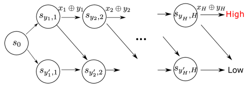
Figure 1: Illustration of the MDP $M_{X,Y}$. For $y\in\{0,1\}$, $y^{\prime}$ stands for $1-y$.

Optimality.

For a given min-player’s policy $\nu$, there exists a best response $\mu^{\dagger}$ to it, such that $V_{h}^{\mu^{\dagger},\nu}(s)=V_{h}^{\dagger,\nu}(s):=\sup_{\mu}V_{h}^{\mu,\nu}(s)$ for any step $h\in[H]$ and state $s\in\mathcal{S}_{h}$. Again, a symmetric discussion applies to the best response to a max-player’s policy. The following minimax theorem holds for two-player zero-sum MGs: for any step $h\in[H]$ and state $s\in\mathcal{S}_{h}$,

$$\max_{\mu}\min_{\nu}V_{h}^{\mu,\nu}(s)=\min_{\nu}\max_{\mu}V_{h}^{\mu,\nu}(s).$$

A policy pair $(\mu^{\ast},\nu^{\ast})$ that achieves the equality is known as a Nash equilibrium. We use $V^{\ast}_{h}(s):=V_{h}^{\mu^{\ast},\nu^{\ast}}(s)$ to denote the value at the Nash equilibrium, which is unique for the MG and we call the minimax value of the MG.

2.2 Problem setup

We are now ready to formally define the problem of online learning in an unknown MG: we control the max-player and in each step, only the state $s_{h}$ and return $r_{h}$ are revealed, but not the action of the min-player $b_{h}$. Recall that if $b_{h}$ is also accessible, we call it the informed setting.

Our goal is to maximize the expected cumulative return, or equivalently, to minimize the regret. The conventional definition of regret is to compete against the best fixed policy in hindsight:

$$\textnormal{Regret}^{\prime}(K):=\sup_{\mu}\sum_{k=1}^{K}\bigl{(}V_{1}^{\mu,\nu^{k}}(s_{1}^{k})-V_{1}^{\mu^{k},\nu^{k}}(s_{1}^{k})\bigr{)},$$ (2.1)

where the superscript $k$ denotes the corresponding objects in the $k$th episode. Although we use this compact notation, the regret depends on both $\mu^{k}$ and $\nu^{k}$.

However, even in the informed setting, achieving sublinear regret in this form is computationally hard (Bai et al., 2020). For online learning in unknown MGs, the problem is statistically hard (Section 3), thus is still intractable even if we have infinite computational power.

Therefore, by noting

$$\max_{\mu\in M}V_{1}^{\mu,\nu^{k}}(s_{1}^{k})\geq V_{1}^{\mu^{\ast},\nu^{k}}(s_{1}^{k})\geq V_{1}^{\ast}(s_{1}^{k}),$$

we consider a more modest goal. That is, to minimize the following regret against the minimax value of the game, which has appeared in prior works (Brafman and Tennenholtz, 2002; Xie et al., 2020):

$$\textnormal{Regret}(K):=\sum\nolimits_{k=1}^{K}\bigl{(}V_{1}^{\ast}(s_{1}^{k})-V_{1}^{\mu^{k},\nu^{k}}(s_{1}^{k})\bigr{)}.$$ (2.2)

3 Statistical hardness of online learning in unknown MGs

As mentioned above, we use the minimax value of the game as the benchmark for online learning in unknown MGs. In contrast, in adversarial MDPs (Jin et al., 2019), it is more common to compete against the best policy in hindsight (using regret (2.1)). In this section, we justify our usage of the weaker notion of regret (2.2) by showing that, in general, competing against the best policy in hindsight is statistically intractable. In particular, we show that in this case, the regret has to be either linear in $K$ or exponential in $H$.

Theorem 1 (Statistical hardness for online learning in unknown MGs).

For any $H\geq 2$ and $K\geq 1$, there exists a two-player zero-sum MG with horizon $H$, $|S_{h}|\leq 2$, $|A_{h}|\leq 2$, $|B_{h}|\leq 4$ such that any algorithm for unknown MGs suffers the following worst-case one-sided regret:

$$\sup_{\mu}\sum\nolimits_{k=1}^{K}\Bigl{(}V_{1}^{\mu,\nu^{k}}(s_{1})-\mathbb{E}_{\mu^{k}}V_{1}^{\mu^{k},\nu^{k}}(s_{1})\Bigr{)}\geq\Omega\bigl{(}\min\bigl{\{}\sqrt{2^{H}K},K\bigr{\}}\bigr{)}.$$

In particular, any algorithm has to suffer linear regret unless $K\geq\Omega(2^{H})$.

Here we give a sketch of our proof, while the full proof is deferred to Appendix A.

We start by considering online learning in (single-agent) MDPs, where the reward and transition function in each episode are adversarially determined, and the goal is to compete against the best (fixed) policy in hindsight. In the following lemma we show that this problem is statistically hard; see Lemma 1 in the appendix for its formal statement.

Lemma (informal).

For any algorithm, there exists a sequence of single agent MDPs with horizon $H$, $S=O(H)$ states and $A=O(1)$ actions, such that the regret defined against the best policy in hindsight is $\Omega(\min\{\sqrt{2^{H}K},K\})$.

Remark 1.

The above lemma is different from a previous hardness result in Yadkori et al. (2013), which states that this problem is computationally hard.

We now briefly explain how this family of hard MDPs is constructed, which is inspired by the “combination lock” MDP (Du et al., 2019). Every MDP $M_{X,Y}$ is specified by two $H$-bit strings: $X,Y\in\{0,1\}^{H}$. The states are $\{s_{0,0},s_{0,1},s_{1,1},\cdots,s_{0,H},s_{1,H}\}$. As shown in Figure 1, $M_{X,Y}$ has a layered structure, and the reward is nonzero only at the final layer. The only way to achieve the high reward is to follow the path $s_{0,0}\to s_{y_{1},1}\to\cdots s_{y_{H},H}$. Thus, the corresponding optimal policy is $\pi(s_{w,h})=x_{h}\oplus w$, which is only a function of $X$. Here, $\oplus$ denotes the bitwise exclusive or operator.

Now, in each episode, $Y$ is chosen from a uniform distribution over $\{0,1\}^{H}$ while $X$ is fixed. When the player interacts with $M_{X,Y}$, since $Y$ is uniformly random, it gets no effective feedback from the observed transitions, and the only informative feedback is the reward at the end. However, achieving the high reward requires guessing every bit of $X$ correctly. This “needle in a haystack” situation makes the problem as hard as a multi-armed bandit problem with $2^{H}$ arms. The regret lower bound immediately follows.

Next, we use the hard family of MDPs in Lemma 1 to prove Theorem 1 by reducing the adversarial MDP problem to online learning in unknown MGs. The construction is straightforward. The state space and the action space for the max-player are the same as that in the original MDP family. The min-player has control over the transition function and reward at each step, and executes a policy such that the induced MDP for the max-player is the same as $M_{X,Y}$. This is possible using only $B=O(1)$ actions as $M_{X,Y}$ has a layered structure. Online learning in unknown MGs then simulates the online learning in the adversarial MDP problem, and thus has the same regret lower bound.

Classes of policies. In Section 2, we define the policy $\mu$ by mappings from $\mathcal{S}_{h}$ to a distribution on $\mathcal{A}_{h}$ at each step $h$. Such policies are called Markov policies (Bai et al., 2020). The policies induced by the algorithms in the remaining part of this paper are always Markov policies. However, our lower bound also holds for general policies (Bai et al., 2020). Here, for an informed max-player the input of $\mu_{h}$ can be the history $(s_{1},a_{1},b_{1},r_{1},\cdots,s_{h})$, while for a max-player in an unknown MG the input of $\mu_{h}$ can be the history $(s_{1},a_{1},r_{1},\cdots,s_{h})$. In words, the lower bound holds even for policies that depend on histories.

Regret minimization in self-play. We emphasize that our lower bound applies to online learning in unknown MGs. For the self-play setting, people indeed minimize the strong regret (2.1) as an intermediate step toward PAC guarantees (Bai and Jin, 2020; Bai et al., 2020; Xie et al., 2020). This is possible because in self-play both players are running the policies specified by the algorithm designer. Therefore, they do not need to worry about the adversarial scenario described in the lower bound here.

4 The V-ol algorithm

Algorithm 1 Optimistic Nash V-learning for Online Learning (V-ol)

1:Require: Learning rate $\{\alpha_{t}\}_{t\geq 1}$, exploration bonus $\{\beta_{t}\}_{t\geq 1}$, policy update parameter $\{\eta_{t}\}_{t\geq 1}$

2:Initialize: for any $h\in[H],s\in\mathcal{S}_{h},a\in\mathcal{A}_{h}$, $V_{h}(s)\leftarrow H$, $L_{h}(s,a)\leftarrow 0$, $N_{h}(s)\leftarrow 0$, $\mu_{h}(a|s)\leftarrow 1/|\mathcal{A}_{h}|$.

3:for episode $k=1,\dots,K$ do

4:     Receive $s_{1}$

5:     for step $h=1,\dots,H$ do

6:         Take action $a_{h}\sim\mu_{h}(\cdot|s_{h})$

7:         Observe return $r_{h}$ and next state $s_{h+1}$

8:         Increase counter $t=N_{h}(s_{h})\leftarrow N_{h}(s_{h})+1$

9:         $V_{h}(s_{h})\leftarrow(1-\alpha_{t})V_{h}(s_{h})+\alpha_{t}(r_{h}+V_{h+1}(s_{h+1})+\beta_{t})$

10:         for all actions $a\in\mathcal{A}_{h}$ do

11:              $l_{h}(s_{h},a)\leftarrow(H-r_{h}-V_{h+1}(s_{h+1}))\mathbb{I}(a_{h}=a)/(\mu_{h}(a_{h}|s_{h})+\eta_{t})$

12:              $L_{h}(s_{h},a)\leftarrow(1-\alpha_{t})L_{h}(s_{h},a)+\alpha_{t}l_{h}(s_{h},a)$

13:         end for

14:         Update policy $\mu$ by

$$\mu_{h}(\cdot|s_{h})\leftarrow\frac{\exp\{-\eta_{t}L_{h}(s_{h},\cdot)/\alpha_{t}\}}{\sum_{a}\exp\{-\eta_{t}L_{h}(s_{h},a)/\alpha_{t}\}}$$

15:     end for

16:end for

In this section, we introduce the V-ol algorithm and its regret guarantees for online learning in two-player zero-sum unknown Markov games. We show that not only can we achieve a sublinear regret in this challenging setting, but the regret bound can be independent of the size of the opponent’s action space as well.

The V-ol algorithm.

V-ol is a variant of V-learning algorithms. Bai et al. (2020) first propose V-sp as a near-optimal algorithm for the self-play setting of two-player zero-sum MGs. See the discussion at the end of this section for a detailed comparison between V-ol and V-sp.

In V-ol (Algorithm 1), at each time step $h$, the player interacts with the environment, performs an incremental update to $V_{h}$, and updates its policy $\mu_{h}$. Note that the estimated value function $V_{h}$ is only used for the intermediate loss $l_{h}(s_{h},\cdot)$ in this time step, but not used in decision making. To encourage exploration in less visited states, we add a bonus term $\beta_{t}$. As we will see in Section 6, this update rule is optimistic, i.e., $V_{h}$ is an upper confidence bound (UCB) on the minimax value ${V_{h}^{\ast}}$ of the MG. Then the player samples the action according to the exponentially weighted averaged loss $L_{h}(s_{h},\cdot)$, which is a popular decision rule in adversarial environments (Auer et al., 1995).

Intuition behind V-learning.

Most existing provably efficient tabular RL algorithms learn a Q-table (table consisting of Q-values). However, since state-action pairs are necessary for updating the Q-table, for online learning in MGs, algorithms based on it inevitably require observing the opponent’s actions and are thus inapplicable to unknown MGs. In contrast, V-ol does not need to maintain the Q-table at all and bypasses this challenge naturally.

Moreover, learning a Q-value function in two-player Markov games usually results in a regret or sample complexity that depends on its size $SAB$, whether in the self-play setting, such as VI-ULCB (Bai and Jin, 2020) and Q-sp (Bai et al., 2020), OMNI-VI-offline (Xie et al., 2020), or in the online setting, such as OMNI-VI-online (Xie et al., 2020) and Q-ol (Appendix C). In contrast, V-learning is promising in removing the dependence on $B$, as formalized in Theorem 2.

Note that we analyze Q-ol in Appendix C to more clearly demonstrate V-ol’s advantage of avoiding learning a Q-table. Q-ol is a Q-learning-type algorithm for online MGs adapted from Q-sp. It updates the Q-values by a termporal difference method like V-ol but makes decisions based on the Q-values instead. Therefore, Q-ol applies only to the informed setting and its regret depends on $AB$ (Theorem 4).

Favoring more recent samples.

Despite the above noted advantages of V-learning, the V-sp algorithm (Bai et al., 2020) may have a regret bound that is linear in $K$, as indicated by (4.2) in Theorem 2 and discussed in Section 6 in more detail. To resolve this problem, we adopt a different set of hyperparameters to learn more aggressively by giving more weight to more recent samples. Concretely, for the self-play setting, Bai et al. (2020) specify the following hyperparameters for V-sp:

$$\alpha_{t}=\tfrac{H+1}{H+t},\;\beta_{t}=c\sqrt{\tfrac{H^{4}A\iota}{t}},\;\eta_{t}=\sqrt{\tfrac{\log A}{At}},$$

where $\iota$ is a log factor defined later. For the online setting, we set these hyperparameters as:

$$\alpha_{t}=\tfrac{GH+1}{GH+t},\;\beta_{t}=c\sqrt{\tfrac{GH^{3}A\iota}{t}},\;\eta_{t}=\sqrt{\tfrac{GH\log A}{At}},$$ (4.1)

where $G\geq 1$ is a quantity that we tune. Ostensibly, these changes may appear small, but they are essential to attaining a sublinear regret.

Remark 2.

Compared with $\alpha_{t}=\nicefrac{{1}}{{t}}$, the learning rate $\alpha_{t}=\nicefrac{{H+1}}{{H+t}}$ first proposed in (Jin et al., 2018) already favors more recent samples. Here we go one step further: our algorithm learns even more aggressively by taking $\alpha_{t}=\nicefrac{{GH+1}}{{GH+t}}$ with $G\geq 1$. Moreover, we choose a larger $\eta_{t}$ to make our algorithm care more about more recently incurred loss. $\beta_{t}$ is set accordingly to achieve optimism.

We call this variant of V-learning V-ol, for which we prove the following regret guarantees.

Theorem 2 (Regret bounds).

For any $p\in(0,1)$, let $\iota=\log(\nicefrac{{HSAK}}{{p}})$. If we run V-ol with our hyperparameter specification (4.1) for some large constant $c$ and $G\geq 1$ in an online two-player zero-sum MG, then with probability at least $1-p$, the regret in $K$ episodes satisfies

$$\textnormal{Regret}(K)=\mathcal{O}\bigl{(}\sqrt{GH^{5}SAK\iota}+KH/G+H^{2}S\bigr{)}.$$ (4.2)

In particular, by taking $G=H^{-1}(K/SA)^{\nicefrac{{1}}{{3}}}$ if $K\geq H^{3}SA$ and $G=K^{\nicefrac{{1}}{{3}}}$ otherwise, with probability at least $1-p$, the regret satisfies

$$\textnormal{Regret}(K)=\begin{cases}\tilde{\mathcal{O}}\bigl{(}H^{2}S^{\frac{1}{3}}A^{\frac{1}{3}}K^{\frac{2}{3}}+H^{2}S\bigr{)},\text{ if }K\geq H^{3}SA,\\ \tilde{\mathcal{O}}\bigl{(}\sqrt{H^{5}SA}K^{\frac{2}{3}}+H^{2}S\bigr{)},\text{ otherwise.}\\ \end{cases}$$

Theorem 2 shows that a sublinear regret against the minimax value of the MG is achievable for online learning in unknown MGs. As expected, the regret bound does not depend on the size of the opponent’s action space $B$. This independence of $B$ is particularly significant for large $B$, as is the case where our player plays with multiple opponents. Note that although in Theorem 2 setting the parameter $G$ requires knowledge of $K$ beforehand, we can use a standard doubling trick to bypass this requirement.

Remark 3.

In V-sp the parameter $G$ is set to be $1$. Then our choice of $\eta_{t}$ becomes $\sqrt{\nicefrac{{H\log A}}{{At}}}$, $\sqrt{H}$ times the original policy update parameter. If the other player also adopts the new $\sqrt{\nicefrac{{H\log B}}{{Bt}}}$ policy update parameter, then the sample complexity of V-sp can actually be improved upon (Bai et al., 2020) by an $\sqrt{H}$ factor to $\tilde{\mathcal{O}}(H^{5}S(A+B)/\epsilon^{2})$.

Comparison between V-ol and V-sp.

1. To achieve near-optimal sample complexity in the self-play setting, V-sp needs to construct upper and lower confidence bounds not only for the minimax value of the game, but also for the best response. As a result, it uses a complicated certified policy technique, and it must store the whole history in the past $K$ episodes for resampling from in each step. By comparing with the minimax value directly, we can make V-ol provably efficient without extracting a certified policy. Therefore, V-ol only needs $\mathcal{O}(SAH)$ space instead of $\mathcal{O}(KSAH)$, and the resampling procedure is no more necessary.

2. A key feature of the proof in (Bai et al., 2020) is to make full use of a symmetric structure, which naturally arises because in the self-play setting we can control both players to follow the same learning algorithm. However, this property no longer holds for the online setting, and we must take a different proof route. Algorithmically, we need to learn more aggressively to make V-ol provably efficient.

3. V-ol also works in multi-player general-sum MGs—see Section 5.

5 Multi-player general-sum games

In this section, we extend the regret guarantees of V-ol to multi-player general-sum MGs, demonstrating the generality of our algorithm. Informally, we have the following corollary.

Corollary (informal).

If we run V-ol with our hyperparameter specificified in (4.1) for our player in an online multi-player general-sum MG, then with high probability, for sufficiently large $K$,

$$\textnormal{Regret}(K)=\tilde{\mathcal{O}}\bigl{(}H^{2}S^{\frac{1}{3}}A^{\frac{1}{3}}K^{\frac{2}{3}}+H^{2}S\bigr{)},$$

where $A$ denotes the size of our player’s action space.

The above corollary highlights the significance of removing the dependence on $B$ in the regret bound. In particular, in a multi-player game the size of the opponents’ joint action space $B$ grows exponentially in the number of opponents, whereas the regret of V-ol only depends on the size of our player’s action space $A$. The savings arise because V-ol bypasses the need to learn Q-tables, and the multi-player setting makes no real difference in our analysis. To formally present the construction, we need to first introduce some notation.

Consider the $m$-player general-sum MG

$$\mathrm{MG}_{m}(\mathcal{S},\{\mathcal{A}_{i}\}_{i=1}^{m},\mathbb{P},\{r_{i}\}_{i=1}^{m},H),$$ (5.1)

where $\mathcal{S}$, $H$ follow from the same definition in two-player zero-sum MGs, and

• for each $i\in[m]$, player $i$ has its own action space $\mathcal{A}_{i}=\bigcup_{h\in[H]}\mathcal{A}_{i,h}$ and return function $r_{i}=\{r_{i,h}:\mathcal{S}_{h}\times\bigotimes_{i=1}^{m}\mathcal{A}_{i,h}\to[0,1]\}_{i=1}^{m}$, and aims to maximize its own cumulative return (here $\bigotimes$ denotes the Cartesian product of sets);

• $\mathbb{P}$ is a collection of transition functions $\{\mathbb{P}_{h}:\mathcal{S}_{h}\times\bigotimes_{i=1}^{m}\mathcal{A}_{i,h}\to\Delta(\mathcal{S}_{h+1})\}_{h\in[H]}$.

Like in two-player MGs, let

$$S:=\sup_{h\in[H]}|\mathcal{S}_{h}|,\quad A_{i}:=\sup_{h\in[H]}|\mathcal{A}_{i},h|\text{ for all }i\in[m].$$

Online learning in an unknown multi-player general-sum MG can be reduced to that in a two-player zero-sum MG. Concretely, suppose we are player $1$, then online learning in unknown MGs (5.1) is indistinguishable from that in the two-player zero-sum MG specified by $(\mathcal{S},\mathcal{A}_{1},\mathcal{B},\mathbb{P},r_{1},H)$ where $\mathcal{B}=\bigotimes_{i=2}^{m}\mathcal{A}_{i}$, since we only observe and care about player $1$’s return. For all states $s\in\mathcal{S}_{1}$, define the value function using $r_{1}$ as

$$V_{h}^{\mu,\nu}(s):=\mathbb{E}_{\mu,\nu}[\sum\nolimits_{h^{\prime}=h}^{H}r_{1,h^{\prime}}(s_{h^{\prime}},a_{h^{\prime}},b_{h^{\prime}})|s_{h}=s],$$

and define the minimax value of player $1$ as

$${V_{1}^{\ast}}(s):=\max_{\mu}\min_{\nu}V_{1}^{\mu,\nu}(s)=\min_{\nu}\max_{\mu}V_{1}^{\mu,\nu}(s),$$

which is no larger than the value at the Nash equilibrium of the multi-player general-sum MG. Then we define the regret against the minimax value of player $1$ as

$$\textnormal{Regret}(K):=\sum\nolimits_{k=1}^{K}\bigl{(}{V_{1}^{\ast}}(s_{1}^{k})-V_{1}^{\mu^{k},\nu^{k}}(s_{1}^{k})\bigr{)}.$$

We argue that this notion of regret is reasonable since we have control of only player $1$ and all opponents may collude to compromise our performance. Then immediately we obtain the following corollary from Theorem 2.

Corollary 3 (Regret bound in multi-player MGs).

For any $p\in(0,1)$, let $\iota=\log(\nicefrac{{HSAK}}{{p}})$. If we run V-ol with our hyperparameter specification (4.1) for some large constant $c$ and the above choice of $G$ for player 1 in the online multi-player general-sum MG (5.1), then with probability at least $1-p$, the regret in $K$ episodes satisfies

$$\textnormal{Regret}(K)=\begin{cases}\tilde{\mathcal{O}}\bigl{(}H^{2}S^{\frac{1}{3}}A_{1}^{\frac{1}{3}}K^{\frac{2}{3}}+H^{2}S\bigr{)},\text{ if }K\geq H^{3}SA_{1},\\ \tilde{\mathcal{O}}\bigl{(}\sqrt{H^{5}SA_{1}}K^{\frac{2}{3}}+H^{2}S\bigr{)},\text{ otherwise.}\\ \end{cases}$$

In the online informed setting, the same equivalence to a two-player zero-sum MG holds, since the other players’ actions we observe can be seen as a single action $(a_{i})_{i=2}^{m}$, and whether we observe the other players’ returns does not help us decide our policies to maximize our own cumulative return. In this setting, the regret bound in (Xie et al., 2020) becomes $\tilde{\mathcal{O}}(\sqrt{H^{3}S^{3}\prod_{i=1}^{m}A_{i}^{3}T})$, which depends exponentially on $m$. On the other hand, since the online informed setting has stronger assumptions than online learning in unknown MGs, the $\tilde{\mathcal{O}}(H^{2}S^{\nicefrac{{1}}{{3}}}A_{1}^{\nicefrac{{1}}{{3}}}K^{\nicefrac{{2}}{{3}}})$ regret bound of V-ol carries over, which has no dependence on $m$. This sharp contrast highlights the importance of achieving a regret independent of the size of the opponent’s action space.

Furthermore, since in V-ol we only need to update the value function (which has $HS$ entries), rather than update the Q-table (which has $HS\prod_{i=1}^{m}A_{i}$ entries) as in (Xie et al., 2020), we can also improve the time and space complexity by an exponential factor in $m$.

6 Proof sketch of Theorem 2

In this section, we sketch the proof of Theorem 2. We also highlight an observation that V-ol can perform much better than claimed in Theorem 2. Moreover, we expose the problem with V-sp in the online setting, which explains why we favor more recent samples in V-ol.

In the analysis below, we use a superscript $k$ to signify the corresponding quantities at the beginning of the $k$th episode. To express $V_{h}^{k}$ in Algorithm 1 compactly, we introduce the following quantities.

$$\alpha_{t}^{0}:=\prod\nolimits_{j=1}^{t}(1-\alpha_{j}),\quad\alpha_{t}^{i}:=\alpha_{i}\prod\nolimits_{j=i+1}^{t}(1-\alpha_{j}).$$

Let $t:=N_{h}^{k}(s)$ and suppose $s$ is previously visited at episodes $k^{1},\ldots,k^{t}\leq k$. Then we can express $V_{h}^{k}(s)$ as

$$\alpha_{t}^{0}H+\sum\nolimits_{i=1}^{t}\alpha_{t}^{i}\bigl{(}r_{h}(s,a_{h}^{k^{i}},b_{h}^{k^{i}})+V_{h+1}^{k^{i}}(s_{h+1}^{k^{i}})+\beta_{i}\bigr{)}.$$

It is easy to verify that $\{\alpha_{t}^{i}\}_{i=1}^{t}$ satisfies the normalization property that $\sum_{i=1}^{t}\alpha_{t}^{i}=1$ for any sequence $\{\alpha_{t}\}_{t\geq 1}$ and any $t\geq 1$. Moreover, for $\{\alpha_{t}\}_{t\geq 1}$ specified in (4.1), $\{\alpha_{t}^{i}\}$ has several other desirable properties (Lemma 2), resembling (Jin et al., 2018, Lemma 4.1).

Upper confidence bound (UCB).

In Algorithm 1, by bonus $\beta_{t}$ we ensure that $V_{h}^{k}$ is an entrywise UCB on ${V_{h}^{\ast}}$ using standard techniques (Bai et al., 2020), building on the normalization property of $\{\alpha_{t}^{i}\}_{i=1}^{t}$ and the key V-learning lemma (Lemma 3) based on the regret bound of the adversarial bandit problem we solve to derive the policy update.

Remark 4.

A main difference from the previous UCB framework (e.g., Azar et al. (2017)) is that here the gap between $V_{h}^{k}$ and ${V_{h}^{\ast}}$ is not necessarily diminishing, which partially explains why we do not achieve the conventional $\tilde{\mathcal{O}}(\sqrt{T})$ regret. Concretely, by taking $\mu=\mu^{\ast}$ in the V-learning lemma (Lemma 3), we have

$$V_{h}^{k}(s)-{V_{h}^{\ast}}(s)$$

$$\geq \sum\nolimits_{i=1}^{t}\alpha_{t}^{i}\mathbb{D}_{\mu_{h}^{\ast},\nu_{h}^{k^{i}}}[r_{h}+\mathbb{P}_{h}V_{h+1}^{k^{i}}](s)-\mathbb{D}_{\mu_{h}^{\ast},\nu_{h}^{\ast}}[r_{h}+\mathbb{P}_{h}{V_{h+1}^{\ast}}](s)$$

$$= \sum\nolimits_{i=1}^{t}\alpha_{t}^{i}\mathbb{D}_{\mu_{h}^{\ast},\nu_{h}^{k^{i}}}[\mathbb{P}_{h}(V_{h+1}^{k^{i}}-{V_{h+1}^{\ast}})](s)+\sum\nolimits_{i=1}^{t}\alpha_{t}^{i}(\mathbb{D}_{\mu_{h}^{\ast},\nu_{h}^{k^{i}}}-\mathbb{D}_{\mu_{h}^{\ast},\nu_{h}^{\ast}})[r_{h}+\mathbb{P}_{h}{V_{h+1}^{\ast}}](s)$$

$$\overset{(i)}{\geq} \sum\nolimits_{i=1}^{t}\alpha_{t}^{i}(\mathbb{D}_{\mu_{h}^{\ast},\nu_{h}^{k^{i}}}-\mathbb{D}_{\mu_{h}^{\ast},\nu_{h}^{\ast}})[r_{h}+\mathbb{P}_{h}{V_{h+1}^{\ast}}](s),$$

where $(i)$ follows from the above UCB. If the opponent is weak at some step $h\in[H]$ such that for all episodes $k\in[K]$,

$$(\mathbb{D}_{\mu_{h}^{\ast},\nu_{h}^{k}}-\mathbb{D}_{\mu_{h}^{\ast},\nu_{h}^{\ast}})[r_{h}+\mathbb{P}_{h}{V_{h+1}^{\ast}}](s)\geq C,$$

then $\sum_{k=1}^{K}(V_{h}^{k}(s)-{V_{h}^{\ast}}(s))\geq CK$. This indicates that the gap between the sum of the UCBs and that of the minimax values can be linear in $K$. As proved below, we actually show that $\sum\nolimits_{k=1}^{K}(V_{1}^{k}-V_{1}^{\mu^{k},\nu^{k}})(s_{h}^{k})$ is sublinear in $K$, which is much stronger than that merely the regret is sublinear if the opponent is weak. In words, V-ol performs much better than claimed in Theorem 2 against a weak opponent.

Regret bounds.

Note that the above proof of the UCB holds for any $G>0$. We now illustrate what problem appears if $G=1$ and where the constraint $G\geq 1$ comes from. Let “$\lesssim$” denote “$\leq$” up to multiplicative constants and log factors. By definition, we have

$$\delta_{h}^{k}:=(V_{h}^{k}-V_{h}^{\mu^{k},\nu^{k}})(s_{h}^{k})\lesssim\sqrt{\tfrac{GH^{3}A\iota}{t}}-\mathbb{D}_{\mu_{h}^{k},\nu_{h}^{k}}[r_{h}+\mathbb{P}_{h}V_{h+1}^{\mu^{k},\nu^{k}}](s_{h}^{k})+\sum\nolimits_{i=1}^{t}\alpha_{t}^{i}\mathbb{D}_{\mu^{k^{i}},\nu^{k^{i}}}[r_{h}+\mathbb{P}_{h}V_{h+1}^{k^{i}}](s_{h}^{k}).$$

By the same regrouping technique as that in Jin et al. (2018), for any quantity $f^{i}$ indexed by $i\in[K]$,

$$\sum\nolimits_{k=1}^{K}\sum\nolimits_{i=1}^{t}\alpha_{t}^{i}f^{k^{i}}\leq\sum\nolimits_{k^{\prime}=1}^{K}f^{k^{\prime}}\sum\nolimits_{t=n_{h}^{k^{\prime}}}^{\infty}\alpha_{t}^{n_{h}^{k^{\prime}}}\leq(1+\tfrac{1}{GH})\sum\nolimits_{k=1}^{K}f^{k}.$$

Taking $\mathbb{D}_{\mu^{k^{i}},\nu^{k^{i}}}[r_{h}+\mathbb{P}_{h}V_{h+1}^{k^{i}}](s_{h}^{k})$ as $f^{i}$ and substituting the resulting bound into $\sum_{k=1}^{K}\delta_{h}^{k}$ yields

$$\sum\nolimits_{k=1}^{K}\delta_{h}^{k} \lesssim\sum\nolimits_{k=1}^{K}\bigl{(}\sqrt{\tfrac{GH^{3}A\iota}{t}}+(1+\tfrac{1}{GH})\delta_{h+1}^{k}+\tfrac{1}{GH}\mathbb{D}_{\mu_{h}^{k},\nu_{h}^{k}}[r_{h}+\mathbb{P}_{h}V_{h+1}^{\mu^{k},\nu^{k}}](s_{h}^{k})\bigr{)}$$

$$\overset{(i)}{\leq}\sum\nolimits_{k=1}^{K}\bigl{(}\sqrt{\tfrac{GH^{3}A\iota}{t}}+(1+\tfrac{1}{GH})\delta_{h+1}^{k}+\tfrac{1}{G}\bigr{)},$$

where $(i)$ is owing to $\mathbb{D}_{\mu_{h}^{k},\nu_{h}^{k}}[r_{h}+\mathbb{P}_{h}V_{h+1}^{\mu^{k},\nu^{k}}](s_{h}^{k})\leq H$. Since $\sum_{k=1}^{K}\delta_{H+1}^{k}=0$, a recursion over $h\in[H]$ for $\sum_{k=1}^{K}\delta_{h}^{k}$ yields

$$\sum\nolimits_{k=1}^{K}\delta_{1}^{k}\lesssim(1+\tfrac{1}{GH})^{H}\bigl{(}\sqrt{\tfrac{GH^{3}A\iota}{t}}+\tfrac{1}{G}\bigr{)}.$$

To bound the coefficient $(1+\tfrac{1}{GH})^{H}\leq e$, we need $G\geq 1$. By noting

$$\sum\nolimits_{k=1}^{K}\sqrt{\tfrac{1}{t}}=\sum\nolimits_{k=1}^{K}\sqrt{\tfrac{1}{n_{h}^{k}}}\leq\sqrt{SK},$$

we obtain

$$\textnormal{Regret}(K)\leq\sum_{k=1}^{K}\delta_{1}^{k}\lesssim\sqrt{GH^{5}SAK\iota}+G^{-1}KH.$$

If we take $G=1$ as in V-sp, the regret is linear in $K$ and therefore useless. To address this problem, we introduced the tunable parameter $G\geq 1$ that balances the $\sqrt{K}$ and $K$ terms in the above bound to yield a sublinear regret.

7 Conclusion and Future Work

In this paper, we study online learning in unknown Markov games using V-ol, which is based on the V-sp algorithm of Bai et al. (2020). V-ol achieves $\tilde{\mathcal{O}}(K^{\nicefrac{{2}}{{3}}})$ regret after $K$ episodes. Furthermore, the regret bound is independent of the size of opponents’ action space. It is still unclear whether one can achieve a sharper regret bound, which is a question worthy of future study. We briefly comment on two other future directions.

Toward $\tilde{\mathcal{O}}(K^{\nicefrac{{1}}{{2}}})$ regret in MDPs. A key reason why we need to learn more aggressively in online learning is that a symmetric structure (like in the proof of V-sp) is absent. However, it exists if the opponent plays a fixed policy, in which case the Markov game becomes an MDP. To see why, we can imagine the opponent is also executing V-ol, which makes no difference since $B=1$. However, even in that case, a gap remains: we can only upper and lower bound $V^{*}$ but not $V_{h}^{\mu^{k},\nu^{k}}$. Figuring out how to fill this gap will make V-ol become the first policy-based algorithm without an estimation of Q-value functions that achieves a $\tilde{\mathcal{O}}(K^{\nicefrac{{1}}{{2}}})$ regret for tabular RL.

Strong regret for MDPs with adversarial rewards. Another special case is MDPs with adversarial rewards, where the transitions are fixed across episodes. In this case, achieving sublinear regret using strong regret (2.1) is possible (Jin et al., 2019). A question is then: does V-ol (or its variants) achieve sublinear regret using the strong regret? Given the many technical differences between adversarial MDPs and online Markov games, it is desirable to resolve these problems in a unified manner. In addition, the form of the model-free update in V-ol should be of independent interest for MDPs with adversarial rewards.

Appendix A Proof of the lower bound

The lower bound builds on the following lower bound for adversarial MDPs where both the transition and the reward function of each episode are chosen adversarially. Note that in our proof of Lemma 1, the optimal policies for $M_{k}$ are the same, so Lemma 1 indeed implies a lower bound on the regret defined against the best stationary policy in hindsight.

Lemma 1 (Lower bound for adversarial MDPs).

For any horizon $H\geq 2$ and $K\geq 1$, there exists a family of MDPs $\mathcal{M}$ with horizon $H$, state space $\{S_{h}\}_{h\leq H}$ with $|S_{h}|\leq 2$, action space ${\left\{A_{h}\right\}}_{h\leq H}$ with $|A_{h}|\leq 2$, and reward $r_{h}\in[0,1]$ such that the following is true: for any algorithm that deploys policy $\mu^{k}$ in episode $k$, we have

$$\sup_{M_{1},\cdots,M_{K}\in\mathcal{M}}\sup_{\mu}\sum_{k=1}^{K}\left(V^{\mu}_{M_{k}}(s_{0})-\mathbb{E}_{\mu_{k}}V^{\mu^{k}}_{M_{k}}(s_{0})\right)\geq\Omega(\min{\left\{\sqrt{2^{H}K},K\right\}}),$$

where $V^{\ast}_{M_{k}}$ refers to the optimal value function of MDP $M_{k}$.

Proof.

Our construction is inspired by the “combination lock” MDP (Du et al., 2019). Let us redefine the horizon length as $H+1$ (so that $H\geq 1$) and let $h$ start from 0. We now define our family of MDPs.

Definition 1 (MDP $M_{X,Y,\varepsilon}$).

For any pair of bit strings $X=(x_{1},\dots,x_{H})\in{\left\{0,1\right\}}^{H}$, $Y=(y_{1},\dots,y_{H})\in{\left\{0,1\right\}}^{H}$ and any $\varepsilon\in(0,1)$, the MDP $M_{X,Y,\varepsilon}$ is defined as follows.

1. The state space is $S_{0}={\left\{s_{0}\right\}}$ and $S_{h}={\left\{s_{0,h},s_{1,h}\right\}}$ for all $1\leq h\leq H$. The MDP starts at $s_{0}$ deterministically and terminates at $s_{0,H}$ or $s_{1,H}$.

2. The action space is $A_{h}={\left\{0,1\right\}}$ for all $0\leq h\leq H$.

3. The transition is defined as follows:

   • $s_{0}$ transitions to $s_{0,1}$ or $s_{1,1}$ with probability at least $1/2$ each, regardless of the action taken.

   • For any $1\leq h\leq H-1$, $s_{y_{h},h}$ transitions to $s_{y_{h+1},h+1}$ deterministically if $a_{h}=x_{h}\oplus y_{h}$ (“correct state” in combination lock), and transitions to $s_{1-y_{h+1},h+1}$ deterministically if $a_{h}=1-x_{h}\oplus y_{h}$.

   • For any $1\leq h\leq H-1$, $s_{1-y_{h},h}$ transitions to $s_{1-y_{h+1},h+1}$ deterministically regardless of the action taken (“wrong state” in combination lock).

4. The reward is $r_{h}\equiv 0$ for all $0\leq h\leq H-1$. At step $H$, we have

   • $r_{H}(s_{y_{H},H})\sim{\sf Ber}(1/2+\varepsilon)$,

   • $r_{H}(s_{1-y_{H},H})\sim{\sf Ber}(1/2-\varepsilon)$.

A visualization for the MDP specified by $X$, $Y$ and $\varepsilon$ is shown in Figure 2.

Figure 2: $M(X,Y)$: “Combination lock” MDP specified by $X$ and $Y$. For $y\in\{0,1\}$, $y^{\prime}$ stands for $1-y$.

It is straightforward to see that the optimal value function of this MDP is $1/2(1/2+\varepsilon)+1/2(1/2-\varepsilon)=1/2$, and the only way to achieve higher reward than $1/2-\varepsilon$ is by following the path of “good states”: $(s_{0},s_{y_{1},1},\cdots,s_{y_{h},h},\cdots,s_{y_{H},H})$. The corresponding optimal policy is $\pi^{\ast}(s_{w,h})=w\oplus x_{h}$, which is independent of $Y$.

Random sequence of MDPs is as hard as a $2^{H}$-armed bandit.

We now consider any fixed (but unknown) $X\in{\left\{0,1\right\}}^{H}$ and draw $K$ independent samples $Y_{k}\sim{\sf Unif}({\left\{0,1\right\}}^{H})$ for $1\leq k\leq K$. We argue that if we provide $M_{k}\mathrel{\mathop{:}}=M_{X,Y_{k},\varepsilon}$ in episode $k$ (with some appropriate choice of $\varepsilon$), then the problem is as hard as a $2^{H}$-armed bandit problem with (minimum) suboptimality gap $\varepsilon$, and thus must have the desired regret lower bound.

Our first claim is that, on average over $Y_{k}$, the trajectory seen by the algorithm is equivalent (equal in distribution) to the following “completely random” MDP: each state $s_{{\left\{0,1\right\}},h}$ transitions to $s_{{\left\{0,1\right\}},h+1}$ with probability at least $1/2$ regardless of the actions taken; and the reward is $r_{H}\sim{\sf Ber}(1/2)$ if $A=X\oplus Y$ and $r_{H}\sim{\sf Ber}(1/2-\varepsilon)$ if $A\neq X\oplus Y$, where $A={\left\{a_{1},\dots,a_{h}\right\}}$ are the actions taken in steps 1 through $H$. Indeed, consider the transition starting from $s_{y_{h},h}$. Since $y_{h+1}\sim{\sf Ber}(1/2)$, the transition probability to $s_{0,h+1}$ and $s_{1,h+1}$ must be $1/2$ each, regardless of the action taken. The claim about the reward follows from the definition of the MDP.

We now construct a bandit instance, and show that solving this bandit problem can be reduced to online learning in the sequence of MDPs above. The bandit instance has $2^{H}$ arms indexed by ${\left\{0,1\right\}}^{H}$. The arm indexed by $X$ gives reward ${\sf Ber}(1/2)$, and otherwise the reward is ${\sf Ber}(1/2-\varepsilon)$. Now, for any algorithm solving the adversarial MDP problem, consider the following induced algorithm for the bandit problem.

Algorithm 2 Reducing bandits to adversarial MDPs

1:for $k=1,\dots,K$ do

2:     Sample $Y\sim{\sf Unif}({\left\{0,1\right\}}^{H})$.

3:     Simulate the adversarial MDP algorithm by showing the trajectory $(s_{0},s_{y_{1},1},\dots,s_{y_{H},H})$.

4:     Denote the action sequence by $A=(a_{1},\dots,a_{H})$.

5:     Play $A\oplus Y$ in the bandit environment.

6:     Show the received bandit reward to the adversarial MDP algorithm as the last step reward.

7:end for

We now argue that the interaction seen by the adversarial MDP algorithm is identical in distribution to the sequence $M_{X,Y_{k},\varepsilon}$. The trajectory is drawn from a uniform distribution, which is the same as that generated by $M_{X,Y_{k},\varepsilon}$. The reward is high, i.e. ${\sf Ber}(1/2)$, if and only if $A\oplus Y=X$, which is equivalent to $A=X\oplus Y$. This is also the case in the adversarial MDP problem, since playing the action sequence $X\oplus Y$ corresponds to playing the optimal policy $\pi^{*}(s_{y_{h},h})=x_{h}\oplus y_{h}$.

Therefore, the regret achieved by the induced algorithm in the bandit environment would be equal (in distribution) to the regret achieved by this algorithm in the adversarial MDP environment. Applying classical lower bounds on stochastic bandits (Lattimore and Szepesvári, 2020, Chapter 15) (which corresponds to taking $\varepsilon=\varepsilon_{H,K}\mathrel{\mathop{:}}=\min{\left\{\sqrt{2^{H}/K},1/4\right\}}$), we obtain

$$\sup_{X\in{\left\{0,1\right\}}^{H}}\mathbb{E}_{Y_{1},\dots,Y_{k}\sim{\sf Unif}({\left\{0,1\right\}}^{H})}{\left[\sum_{k=1}^{K}\left(V^{\ast}_{M_{X,Y_{k},\varepsilon_{H,K}}}(s_{0})-\mathbb{E}_{\mu^{k}}V^{\mu^{k}}_{M_{X,Y_{k},\varepsilon_{H,K}}}(s_{0})\right)\right]}\geq\Omega(\min{\left\{\sqrt{2^{H}K},K\right\}}),$$

where $\mathbb{E}_{\mu^{k}}$ denotes the randomness in the algorithm execution (which includes the randomness of the realized transitions and rewards that were used by the algorithm to determine $\mu^{k}$). Note that for the MDP $M_{X,Y_{k},\epsilon_{H},T}$, the optimal policy is dictated by $X$ and independent of $Y_{k}$ (hence independent of $k$). Thus, the previous lower bound can rewritten as a comparison with the best policy in hindsight:

$$\sup_{X\in{\left\{0,1\right\}}^{H}}\sup_{\mu}\mathbb{E}_{Y_{1},\dots,Y_{k}\sim{\sf Unif}({\left\{0,1\right\}}^{H})}{\left[\sum_{k=1}^{K}\left(V^{\mu}_{M_{X,Y_{k},\varepsilon_{H,K}}}(s_{0})-\mathbb{E}_{\mu^{k}}V^{\mu^{k}}_{M_{X,Y_{k},\varepsilon_{H,K}}}(s_{0})\right)\right]}\geq\Omega(\min{\left\{\sqrt{2^{H}K},K\right\}}).$$

The adversarial MDP problem is as hard as the above random sequence of MDPs.

Define $\mathcal{M}\mathrel{\mathop{:}}={\left\{M_{X,Y,\varepsilon_{H,K}}:X,Y\in{\left\{0,1\right\}}^{H}\right\}}$. As the minimax regret is lower bounded by the average regret over any prior distribution of MDPs, the above lower bound implies the following minimax lower bound

$$\sup_{M_{k}\in\mathcal{M}}\sup_{\mu}{\left[\sum_{k=1}^{K}\left(V^{\mu}_{M_{k}}(s_{0})-\mathbb{E}_{\mu^{k}}V^{\mu^{k}}_{M_{k}}(s_{0})\right)\right]}\geq\Omega(\min{\left\{\sqrt{2^{H}K},K\right\}})$$

for any adversarial MDP algorithm. ∎

Proof of Theorem 1.

With Lemma 1 in hand, we are in a position to prove the main theorem.

Our proof follows by defining a two-player Markov game and a set of min-player policies ${\left\{\nu^{k}\right\}}$ such that the transitions and rewards seen by the max-player are exactly equivalent to the MDP $M_{X,Y_{k},\varepsilon_{H,K}}$ constructed in Lemma 1. Indeed, we augment the MDP $M_{X,Y_{k},\varepsilon_{H,K}}$ with a set of min-player actions $\mathcal{B}_{h}={\left\{1,2,3,4\right\}}$, and redefine the transition such that from any $s_{i,h}$ where $i\in{\left\{0,1\right\}}$ and $1\leq h\leq H-1$, the Markov game transitions according to Table 1.

$a$/$b$	$1$	$2$	$3$	$4$
$0$	$s_{i,h+1}$	$s_{1-i,h+1}$	$s_{i,h+1}$	$s_{1-i,h+1}$
$1$	$s_{i,h+1}$	$s_{1-i,h+1}$	$s_{1-i,h+1}$	$s_{i,h+1}$

Table 1: transition function of the state $s_{i,h}$ for the hard instance of Markov games.

Such an action set $\mathcal{B}_{h}$ is powerful enough to reproduce all the possible transitions in the original single-player MDP. We then define $\nu^{k}$ as the policy such that the transition follows exactly $M_{X,Y_{k}}$. The reward function is determined only by states and thus remains the same. Therefore, Lemma 1 implies the following one-sided regret bound for the max-player:

$$\sup_{\nu^{k}}\sup_{\mu}\sum_{k=1}^{K}\left(V^{\mu,\nu^{k}}(s_{0})-\mathbb{E}_{\mu^{k}}V^{\mu^{k},\nu^{k}}(s_{0})\right)\geq\Omega(\min{\left\{\sqrt{2^{H}K},K\right\}}),$$

which is the desired result. ∎

Appendix B Proof for the V-ol algorithm

Throughout this section, let $\iota=\log(\nicefrac{{HSAK}}{{p}})$. The following lemma summarizes the key properties of the choice of the learning rate $\alpha_{t}$, which are used in the proof below.

Lemma 2 ((Jin et al., 2018, Lemma 4.1)).

The following properties hold for $\alpha_{t}^{i}$.

1. $\nicefrac{{1}}{{\sqrt{t}}}\leq\sum_{i=1}^{t}\nicefrac{{\alpha_{t}^{i}}}{{\sqrt{i}}}\leq\nicefrac{{2}}{{\sqrt{t}}}$ for all $t\geq 1$.

2. $\sum_{i=1}^{t}(\alpha_{t}^{i})^{2}\leq\max_{i\in[t]}\alpha_{t}^{i}\leq\nicefrac{{2GH}}{{t}}$ for all $t\geq 1$.

3. $\sum_{t=i}^{\infty}\alpha_{t}^{i}=1+\nicefrac{{1}}{{GH}}$ for all $i\geq 1$.

B.1 Upper confidence bound on the minimax value function

Lemma 3 (V-learning lemma).

In Algorithm 1, let $t=N_{h}^{k}(s)$ and suppose state $s\in\mathcal{S}_{h}$ was previously visited at episodes $k^{1},\ldots,k^{t}<k$ at the $h$th step. For any $p\in(0,1)$, let $\iota=\log(\nicefrac{{HSAK}}{{p}})$. Choose $\eta_{t}=\sqrt{\nicefrac{{GH\log A}}{{At}}}$. Then with probability at least $1-p$, for any $t\in[K]$, $h\in[H]$ and $s\in\mathcal{S}_{h}$, there exists a constant $c$ such that

$$\max_{\mu\in\Delta_{\mathcal{A}}}\sum_{i=1}^{t}\alpha_{t}^{i}\mathbb{D}_{\mu,\nu_{h}^{k^{i}}}\left[r_{h}+\mathbb{P}_{h}V_{h+1}^{k^{i}}\right](s)-\sum_{i=1}^{t}\alpha_{t}^{i}\left(r_{h}(s,a_{h}^{k^{i}},b_{h}^{k^{i}})+V_{h+1}^{k^{i}}(s_{h+1}^{k^{i}})\right)\leq c\sqrt{GH^{3}A\iota/t}.$$ (B.1)

Proof.

By the Azuma-Hoeffding inequality and Lemma 2,

$$\sum_{i=1}^{t}{\alpha_{t}^{i}\mathbb{D}_{\mu_{h}^{k^{i}}\times\nu_{h}^{k^{i}}}\left(r_{h}+\mathbb{P}_{h}V_{h+1}^{k^{i}}\right)\left(s\right)}-\sum_{i=1}^{t}{\alpha_{t}^{i}\left[r_{h}\left(s,a_{h}^{k^{i}},b_{h}^{k^{i}}\right)+V_{h+1}^{k^{i}}\left(s_{h+1}^{k^{i}}\right)\right]}\leq 2\sqrt{GH^{3}\iota/t}.$$

So we only need to bound

$$R_{t}^{\ast}:=\underset{\mu\in\Delta_{\mathcal{A}}}{\max}\sum_{i=1}^{t}{\alpha_{t}^{i}\mathbb{D}_{\mu\times\nu_{h}^{k^{i}}}\left(r_{h}+\mathbb{P}_{h}V_{h+1}^{k^{i}}\right)\left(s\right)}-\sum_{i=1}^{t}{\alpha_{t}^{i}\mathbb{D}_{\mu_{h}^{k^{i}}\times\nu_{h}^{k^{i}}}\left(r_{h}+\mathbb{P}_{h}V_{h+1}^{k^{i}}\right)\left(s\right)}.$$ (B.2)

By taking $w_{i}=\alpha_{t}^{i}$ in (Bai et al., 2020, Lemma 17),

$$R_{t}^{\ast}\leq \frac{3H\alpha_{t}^{t}\log A}{\eta_{t}}+\frac{3A}{2}\sum\nolimits_{i=1}^{t}{\eta_{i}}\alpha_{t}^{i}+\sqrt{2\iota\sum\nolimits_{i=1}^{t}{\left(\alpha_{t}^{i}\right)^{2}}}$$

$$\overset{(i)}{\leq} 3H\alpha_{t}^{t}\sqrt{\tfrac{At\log A}{GH}}+\frac{3}{2}\sqrt{GHA\log A}\sum\nolimits_{i=1}^{t}{\frac{\alpha_{t}^{i}}{\sqrt{i}}}+\sqrt{2\iota\sum\nolimits_{i=1}^{t}{\left(\alpha_{t}^{i}\right)^{2}}}$$

$$\overset{(ii)}{\leq} 3H\tfrac{GH+1}{GH+t}\sqrt{\tfrac{At\log A}{GH}}+3\sqrt{\tfrac{GHA\log A}{t}}+2\sqrt{\tfrac{GH\iota}{t}}$$

$$\leq c\sqrt{\tfrac{GHA\iota}{t}}$$

for some constant $c$, where $(i)$ is by setting $\eta_{t}=\sqrt{\frac{GH\log A}{At}}$ and $(ii)$ is by Lemma 2. Taking union bound w.r.t. all $(t,s,h)\in[K]\times\mathcal{S}\times[H]$ concludes the proof.

We comment that the quantity $R_{t}^{*}$ is actually $H$ times the LHS in the inequality of (Bai et al., 2020, Lemma 17). See Appendix F and Algorithm 9 in Bai et al. (2020) for a detailed reduction from MG to adversarial bandit problem. Furthermore, in (Bai et al., 2020) there are actually two parameters $\eta_{t}$ and $\gamma_{t}$. Here we just take $\gamma_{t}=\eta_{t}$ for simplicity. Finally, the proof of (Bai et al., 2020, Lemma 17) requires that $\eta_{i}\leq 2\gamma_{i}$ for all $i\leq t$ (Bai et al., 2020, Lemma 19) and that $\gamma_{t}$ is nondecreasing in $t$ (Bai et al., 2020, Lemma 21), which are both satisfied by our specification of $\eta_{t}$. ∎

Lemma 4 (Upper confidence bound).

In Algorithm 1, for any $p\in(0,1)$, let $\iota=\log(\nicefrac{{HSAK}}{{p}})$ and choose $\beta_{t}=c\sqrt{GH^{3}A\iota/t}$ for some large constant $c$. Then with probability at least $1-p$, ${V_{h}^{\ast}}(s)\leq V_{h}^{k}(s)$ for all $k\in[K]$, $h\in[H]$ and $s\in\mathcal{S}_{h}$.

Proof.

The proof is similar to that of (Bai et al., 2020, Lemma 15), except that we need to deal with an extra parameter $G$ here.

Let $k_{h}^{i}(s)$ denote the index of the episode where $s\in\mathcal{S}_{h}$ is observed at step $h$ for the $i$th time. Where there is no ambiguity, we use $k^{i}$ as a shorthand for $k_{h}^{i}(s)$. Let $s_{h}^{k}$ be the state actually observed in the algorithm at step $h$ in episode $k$. For our choice of $\beta_{i}$, we have $\sum_{i=1}^{t}\alpha_{t}^{i}\beta_{i}=\Theta(GH^{2}\sqrt{\nicefrac{{A\iota}}{{t}}})$ by Lemma 2.

Recall that

$$V_{h}^{k}(s) :=\alpha_{t}^{0}H+\sum_{i=1}^{t}\alpha_{t}^{i}\left(r_{h}(s,a_{h}^{k^{i}},b_{h}^{k^{i}})+V_{h+1}^{k^{i}}(s_{h+1}^{k^{i}})+\beta_{i}\right),$$

$${V_{h}^{\ast}}(s) :=\mathbb{D}_{\mu_{h}^{\ast},\nu_{h}^{\ast}}[r_{h}+\mathbb{P}_{h}{V_{h+1}^{\ast}}](s).$$

For $h=H+1$ the UCB vacuously holds. To apply backward induction, assume that ${V_{h+1}^{\ast}}\leq V_{h+1}^{k}$ holds entrywise. Then by definition, for any $s\in\mathcal{S}_{h}$,

$${V_{h}^{\ast}}(s) =\max_{\mu\in\Delta_{\mathcal{A}_{h}}}\min_{\nu\in\Delta_{\mathcal{B}_{h}}}\mathbb{D}_{\mu,\nu}[r_{h}+\mathbb{P}_{h}{V_{h+1}^{\ast}}](s)$$

$$\overset{(i)}{=}\max_{\mu\in\Delta_{\mathcal{A}_{h}}}\sum\nolimits_{i=1}^{t}\alpha_{t}^{i}\min_{\nu\in\Delta_{\mathcal{B}_{h}}}\mathbb{D}_{\mu,\nu}[r_{h}+\mathbb{P}_{h}{V_{h+1}^{\ast}}](s)$$

$$\leq\max_{\mu\in\Delta_{\mathcal{A}_{h}}}\sum\nolimits_{i=1}^{t}\alpha_{t}^{i}\mathbb{D}_{\mu,\nu_{h}^{k^{i}}}[r_{h}+\mathbb{P}_{h}{V_{h+1}^{\ast}}](s)$$

$$\overset{(ii)}{\leq}\max_{\mu\in\Delta_{\mathcal{A}_{h}}}\sum\nolimits_{i=1}^{t}\alpha_{t}^{i}\mathbb{D}_{\mu,\nu_{h}^{k^{i}}}[r_{h}+\mathbb{P}_{h}V_{h+1}^{k^{i}}](s)\overset{(iii)}{\leq}V_{h}^{k}(s),$$

where $(i)$ follows from $\sum_{i=1}^{t}\alpha_{t}^{i}=1$, in $(ii)$ we apply the induction assumption, and $(iii)$ holds with probability at least $1-p$ by the V-learning lemma (Lemma 3) and that $\sum_{i=1}^{t}\alpha_{t}^{i}\beta_{t}=\Theta(\sqrt{GH^{3}A\iota/t})$ because of our choice of $\beta_{t}$ and Property 1 of $\{\alpha_{t}^{i}\}$ in Lemma 2. Inductively we have ${V_{h}^{\ast}}(s)\leq V_{h}^{k}(s)$ for all $k\in[K]$, $h\in[H]$ and $s\in\mathcal{S}_{h}$. ∎

B.2 Proof of Theorem 2

Proof.

In the proof below, we use ‘$\lesssim$’ to denote ‘$\leq$’ hiding some constants. Recall that

$$V_{h}^{\mu^{k},\nu^{k}}(s_{h}^{k})=\mathbb{D}_{\mu_{h}^{k},\nu_{h}^{k}}[r_{h}+\mathbb{P}_{h}V_{h+1}^{\mu^{k},\nu^{k}}](s_{h}^{k}).$$

Then define $\delta_{h}^{k}:=(V_{h}^{k}-V_{h}^{\mu^{k},\nu^{k}})(s_{h}^{k})$. By definition,

$$\delta_{h}^{k} =\alpha_{t}^{0}H+\sum_{i=1}^{t}\alpha_{t}^{i}\left(r_{h}(s_{h}^{k},a_{h}^{k^{i}},b_{h}^{k^{i}})+V_{h+1}^{k^{i}}(s_{h+1}^{k^{i}})+\beta_{i}\right)-\mathbb{D}_{\mu_{h}^{k},\nu_{h}^{k}}[r_{h}+\mathbb{P}_{h}V_{h+1}^{\mu^{k},\nu^{k}}](s_{h}^{k})$$

$$\overset{(i)}{=}\alpha_{t}^{0}H+\sum_{i=1}^{t}\alpha_{t}^{i}\left(r_{h}(s_{h}^{k},a_{h}^{k^{i}},b_{h}^{k^{i}})+V_{h+1}^{k^{i}}(s_{h+1}^{k^{i}})+\beta_{i}\right)-\sum_{i=1}^{t}\alpha_{t}^{i}\mathbb{D}_{\mu^{k^{i}},\nu^{k^{i}}}[r_{h}+\mathbb{P}_{h}V_{h+1}^{k^{i}}](s_{h}^{k})$$

$$\qquad\qquad+\sum_{i=1}^{t}\alpha_{t}^{i}\mathbb{D}_{\mu^{k^{i}},\nu^{k^{i}}}[r_{h}+\mathbb{P}_{h}V_{h+1}^{k^{i}}](s_{h}^{k})-\mathbb{D}_{\mu_{h}^{k},\nu_{h}^{k}}[r_{h}+\mathbb{P}_{h}V_{h+1}^{\mu^{k},\nu^{k}}](s_{h}^{k})$$

$$\overset{(ii)}{\lesssim}\alpha_{t}^{0}H+\sqrt{\tfrac{GH^{3}A\iota}{t}}+\sum_{i=1}^{t}\alpha_{t}^{i}\mathbb{D}_{\mu^{k^{i}},\nu^{k^{i}}}[r_{h}+\mathbb{P}_{h}V_{h+1}^{k^{i}}](s_{h}^{k})-\mathbb{D}_{\mu_{h}^{k},\nu_{h}^{k}}[r_{h}+\mathbb{P}_{h}V_{h+1}^{\mu^{k},\nu^{k}}](s_{h}^{k}),$$

where in $(i)$ we add and subtract the same term, and $(ii)$ follows from the property of $\beta_{i}$ that $\sum_{i=1}^{t}\alpha_{t}^{i}\beta_{i}=\Theta(\sqrt{\nicefrac{{GH^{3}A\iota}}{{t}}})$ and the fact that by the Azuma-Hoeffding inequality and Property 2 of Lemma 2,

$$\sum_{i=1}^{t}\alpha_{t}^{i}\left(r_{h}(s_{h}^{k},a_{h}^{k^{i}},b_{h}^{k^{i}})+V_{h+1}^{k^{i}}(s_{h+1}^{k^{i}})\right)-\sum_{i=1}^{t}\alpha_{t}^{i}\mathbb{D}_{\mu^{k^{i}},\nu^{k^{i}}}[r_{h}+\mathbb{P}_{h}V_{h+1}^{k^{i}}](s_{h}^{k})\lesssim\sqrt{\tfrac{GH^{3}\iota}{t}}.$$

By the same regrouping technique as that in (Jin et al., 2018),

$$\sum_{k=1}^{K}\sum_{i=1}^{t}\alpha_{t}^{i}\mathbb{D}_{\mu^{k^{i}},\nu^{k^{i}}}[r_{h}+\mathbb{P}_{h}V_{h+1}^{k^{i}}](s_{h}^{k}) \leq\sum_{k^{\prime}=1}^{K}\mathbb{D}_{\mu^{k^{\prime}},\nu^{k^{\prime}}}[r_{h}+\mathbb{P}_{h}V_{h+1}^{k^{\prime}}](s_{h}^{k})\sum_{t=n_{h}^{k^{\prime}}}^{\infty}\alpha_{t}^{n_{h}^{k^{\prime}}}$$

$$\leq(1+\tfrac{1}{GH})\sum_{k=1}^{K}\mathbb{D}_{\mu^{k},\nu^{k}}[r_{h}+\mathbb{P}_{h}V_{h+1}^{k}](s_{h}^{k}).$$

Substituting the above back into the bound on $\delta_{h}^{k}$ and taking sum over $k\in[K]$, we obtain

$$\sum_{k=1}^{K}\delta_{h}^{k} \lesssim\sum_{k=1}^{K}\left(\alpha_{t}^{0}H+\sqrt{\tfrac{GH^{3}A\iota}{t}}+(1+\tfrac{1}{GH})\mathbb{D}_{\mu^{k},\nu^{k}}[r_{h}+\mathbb{P}_{h}V_{h+1}^{k}](s_{h}^{k})-\mathbb{D}_{\mu_{h}^{k},\nu_{h}^{k}}[r_{h}+\mathbb{P}_{h}V_{h+1}^{\mu^{k},\nu^{k}}](s_{h}^{k})\right)$$

$$\overset{(i)}{=}\sum_{k=1}^{K}\left(\alpha_{t}^{0}H+\sqrt{\tfrac{GH^{3}A\iota}{t}}+(1+\tfrac{1}{GH})(\delta_{h+1}^{k}+\gamma_{h}^{k})+\tfrac{1}{GH}\mathbb{D}_{\mu_{h}^{k},\nu_{h}^{k}}[r_{h}+\mathbb{P}_{h}V_{h+1}^{\mu^{k},\nu^{k}}](s_{h}^{k})\right)$$

$$\overset{(ii)}{\leq}\sum_{k=1}^{K}\left(\alpha_{t}^{0}H+\sqrt{\tfrac{GH^{3}A\iota}{t}}+(1+\tfrac{1}{GH})(\delta_{h+1}^{k}+\gamma_{h}^{k})+\tfrac{1}{G}\right),$$

where in $(i)$ we define the martingale difference term $\gamma_{h}^{k}:=\mathbb{D}_{\mu_{h}^{k},\nu_{h}^{k}}[\mathbb{P}_{h}(V_{h+1}^{k}-V_{h+1}^{\mu^{k},\nu^{k}})](s_{h}^{k})-(V_{h+1}^{k}-V_{h+1}^{\mu^{k},\nu^{k}})(s_{h+1}^{k})$ and $(ii)$ follows from that

$$\mathbb{D}_{\mu_{h}^{k},\nu_{h}^{k}}[r_{h}+\mathbb{P}_{h}V_{h+1}^{\mu^{k},\nu^{k}}](s_{h}^{k})\leq H.$$

Recursively,

$$\sum_{k=1}^{K}\delta_{1}^{k} \lesssim(1+\tfrac{1}{GH})^{H}\sum_{k=1}^{K}\sum_{h=1}^{H}\left(\alpha_{t}^{0}H+\sqrt{\tfrac{GH^{3}A\iota}{t}}+(1+\tfrac{1}{GH})\gamma_{h}^{k}+\tfrac{1}{G}\right).$$

Now we bound each term in $\sum_{k=1}^{K}\delta_{1}^{k}$ separately by standard techniques in (Jin et al., 2018; Xie et al., 2020):

$$\sum_{k=1}^{K}\alpha_{n_{h}^{k}}^{0}H\leq\sum_{k=1}^{K}H\cdot\mathbb{I}(n_{h}^{k}=0)\leq HS,$$

$$\sum_{k=1}^{K}\sqrt{\tfrac{GH^{3}A\iota}{n_{h}^{k}}}=GH^{2}\sqrt{A\iota}\sum_{k=1}^{K}\sqrt{\tfrac{1}{n_{h}^{k}}}\leq\sqrt{GH^{3}A\iota}\sum_{s\in\mathcal{S}_{h}}\sum_{n=1}^{n_{h}^{K}(s)}\sqrt{\tfrac{1}{n}}\lesssim\sqrt{GH^{3}SAK\iota}),$$

$$\sum_{k=1}^{K}\sum_{h=1}^{H}\gamma_{h}^{k}\lesssim\sqrt{H^{3}K\iota},$$

where the second line follows from a pigeonhole argument and the third line follows from the Azuma-Hoeffding inequality. Combining the above bounds, we obtain

$$\textnormal{Regret}(K)\leq\sum_{k=1}^{K}\delta_{1}^{k}\lesssim H^{2}S+\sqrt{GH^{5}SAK\iota}+G^{-1}KH.$$

If $K\geq H^{3}SA$ then we take we take $G=\frac{1}{H}(\frac{K}{SA})^{\nicefrac{{1}}{{3}}}$; otherwise we take $G=K^{\tfrac{1}{3}}$. Then the following regret bounds holds:

$$\textnormal{Regret}(K)=\begin{cases}\tilde{\mathcal{O}}\bigl{(}H^{2}S^{\frac{1}{3}}A^{\frac{1}{3}}K^{\frac{2}{3}}+H^{2}S\bigr{)},\text{ if }K\geq H^{3}SA,\\ \tilde{\mathcal{O}}\bigl{(}\sqrt{H^{5}SA}K^{\frac{2}{3}}+H^{2}S\bigr{)},\text{ otherwise.}\\ \end{cases}$$

∎

Appendix C The Q-ol Algorithm

When explaining the intuition behind the V-ol in Section 4, we mentioned that learning a Q-table will result in a regret bound depending on $AB$. This is clear for the other algorithms we mentioned in the literature. However, the regret bounds of Q-learning-type algorithms have not been studied to our best knowledge. In this section, we study a Q-learning-type algorithm for online MGs. We formalize V-ol in Algorithm 3, which is similar to the Optimistic Nash Q-learning (Q-sp) algorithm in (Bai et al., 2020). We emphasize that since learning a Q-table requires knowing the opponents’ actions, Q-ol only works for informed MGs, but not for unknown MGs.

Algorithm 3 Optimistic Nash Q-learning for Online Learning (Q-ol)

1:Require: Learning rate $\{\alpha_{t}\}_{t\geq 1}$, exploration bonus $\{\beta_{t}\}_{t\geq 1}$

2:Initialize: for any $(s,a,b,h)$, $Q_{h}(s,a,b)\leftarrow H$, $N_{h}(s,a,b)\leftarrow 0$, $\mu_{h}(a|s)\leftarrow 1/A$

3:for episode $k=1,\dots,K$ do

4:     Receive $s_{1}$

5:     for step $h=1,\dots,H$ do

6:         Take action $a_{h}\sim\mu_{h}(\cdot|s_{h})$

7:         Observe action $b_{h}$, reward $r_{h}(s_{h},a_{h},b_{h})$ and next state $s_{h+1}$

8:         $t=N_{h}(s_{h},a_{h},b_{h})\leftarrow N_{h}(s_{h},a_{h},b_{h})+1$

9:         $Q_{h}(s_{h},a_{h},b_{h})\leftarrow(1-\alpha_{t})Q_{h}(s_{h},a_{h},b_{h})+\alpha_{t}(r_{h}(s_{h},a_{h},b_{h})+V_{h+1}(s_{h+1})+\beta_{t})$

10:         Solve the NE $(\mu_{h}(\cdot,|s_{h}),\nu_{h}(\cdot,|s_{h}))$ of the matrix game with payoff matrix $Q_{h}^{k}(s_{h},\cdot,\cdot)$

11:         $V_{h}(s_{h})\leftarrow(\mathbb{D}_{\mu_{h}\times\nu_{h}}Q_{h})(s_{h})$

12:     end for

13:end for

In Algorithm 3, we set $\alpha_{t}:=\nicefrac{{H+1}}{{H+t}}$. As in the analysis of V-ol, below we use a superscript $k$ to signify the corresponding quantities at the beginning of the $k$th episode. The following lemma claims that $Q_{h}^{k}$ and $V_{h}^{k}$ are the entrywise upper confidence bounds of $Q_{h}^{\ast}$ and ${V_{h}^{\ast}}$ for all $k\in[K]$ and $h\in[H]$; see the proof of (Bai et al., 2020, Lemma 3) for its proof.

Lemma 5 (Upper confidence bounds).

In Algorithm 3, for any $p\in(0,1)$, $\iota=\log(\nicefrac{{HSAK}}{{p}})$ and choose $\beta_{t}=c\sqrt{H^{3}\iota/t}$ for some large constant $c$. Then with probability at least $1-p$, $Q_{h}^{\ast}(s,a,b)\leq Q_{h}^{k}(s,a,b)$ and ${V_{h}^{\ast}}(s)\leq V_{h}^{k}(s)$ for all $k\in[K]$, $h\in[H]$ and $(s,a,b)\in\mathcal{S}\times\mathcal{A}_{h}\times\mathcal{B}_{h}$.

Then for Q-ol, we have the following regret guarantees.

Theorem 4 (Regret bound of Q-ol).

For any $p\in(0,1)$, let $\iota=\log(\nicefrac{{HSAK}}{{p}})$ and choose $\beta_{t}=c\sqrt{H^{3}\iota/t}$ for some large constant $c$. If we run Q-ol in a two-player zero-sum MG, then with probability at least $1-p$, the regret in $K$ episodes satisfies

$$\textnormal{Regret}(K)=\mathcal{O}\left(SABH^{2}+\sqrt{H^{5}SABK\iota}\right).$$ (C.1)

Proof.

Let $k_{h}^{i}(s,a,b)$ denote the index of the episode where $(s,a,b)$ is observed at step $h$ for the $i$th time. Where there is no ambiguity, we use $k^{i}$ as a shorthand for $k_{h}^{i}(s,a,b)$. Let $s_{h}^{k}$ be the state actually observed in the algorithm at step $h$ in episode $k$.

By defining

$$\overline{\gamma}_{h}^{k} :=\mathbb{E}_{a\sim\mu_{h}^{k}(s_{h}^{k})}[Q_{h}^{k}(s_{h}^{k},a,b_{h}^{k})]-Q_{h}^{k}(s_{h}^{k},a_{h}^{k},b_{h}^{k}),$$

$$\hat{\gamma}_{h}^{k} :=\mathbb{E}_{a\sim\mu_{h}^{k}(s_{h}^{k}),b\sim\omega_{h}^{k}}[Q_{h}^{\mu^{k},\omega^{k}}(s_{h}^{k},a,b)]-Q_{h}^{\mu^{k},\omega^{k}}(s_{h}^{k},a_{h}^{k},b_{h}^{k}),$$

we have

$$V_{h}^{k}(s_{h}^{k})=\min_{\nu\in\Delta_{\mathcal{B}}}\mathbb{E}_{a\sim\mu_{h}^{k}(s_{h}^{k}),b\sim\nu}[Q_{h}^{k}(s_{h}^{k},a,b)]\leq\mathbb{E}_{a\sim\mu_{h}^{k}(s_{h}^{k})}[Q_{h}^{k}(s_{h}^{k},a,b_{h}^{k})]=Q_{h}^{k}(s_{h}^{k},a_{h}^{k},b_{h}^{k})+\overline{\gamma}_{h}^{k},$$

$$V_{h}^{\mu^{k},\omega^{k}}(s_{h}^{k})=\mathbb{E}_{a\sim\mu_{h}^{k}(s_{h}^{k}),b\sim\omega_{h}^{k}}[Q_{h}^{\mu^{k},\omega^{k}}(s_{h}^{k},a,b)]=Q_{h}^{\mu^{k},\omega^{k}}(s_{h}^{k},a_{h}^{k},b_{h}^{k})+\hat{\gamma}_{h}^{k}.$$

Define $\delta_{h}^{k}:=V_{h}^{k}(s_{h}^{k})-V_{h}^{\mu^{k},\omega^{k}}(s_{h}^{k})$ and $\phi_{h}^{k}:=V_{h}^{k}(s_{h}^{k})-{V_{h}^{\ast}}(s_{h}^{k})$. Then

$$\delta_{h}^{k}\leq Q_{h}^{k}(s_{h}^{k},a_{h}^{k},b_{h}^{k})+\overline{\gamma}_{h}^{k}-Q_{h}^{\mu^{k},\omega^{k}}(s_{h}^{k},a_{h}^{k},b_{h}^{k})-\hat{\gamma}_{h}^{k}.$$

In Algorithm 3, for any $k\in[K]$, $h\in[H]$ and $(s,a,b)\in\mathcal{S}_{h}\times\mathcal{A}_{h}\times\mathcal{B}_{h}$, let $t:=N_{h}^{k}(s,a,b)$ and suppose $(s,a,b)$ is previously visited at episodes $k^{1},\cdots,k^{t}\leq k$. Then we can rewrite $Q_{h}^{k}(s,a,b)$ as

$$Q_{h}^{k}(s,a,b)=\alpha_{t}^{0}H+\sum_{i=1}^{t}\alpha_{t}^{i}\left(r_{h}(s,a,b)+V_{h+1}^{k^{i}}(s_{h+1}^{k^{i}})+\beta_{i}\right),$$

and recall that

$$Q_{h}^{\ast}(s,a,b)=r_{h}(s,a,b)+\mathbb{P}_{h}{V_{h+1}^{\ast}}(s,a,b).$$

Then the difference between $Q_{h}^{k}$ and $Q_{h}^{\mu^{k},\omega^{k}}$ at $(s_{h}^{k},a_{h}^{k},b_{h}^{k})$ satisfies

$$(Q_{h}^{k}-Q_{h}^{\mu^{k},\omega^{k}})(s_{h}^{k},a_{h}^{k},b_{h}^{k}) \overset{(i)}{=}(Q_{h}^{k}-Q_{h}^{\ast}+Q_{h}^{\ast}-Q_{h}^{\mu^{k},\omega^{k}})(s_{h}^{k},a_{h}^{k},b_{h}^{k})$$

$$\overset{(ii)}{\leq}\alpha_{t}^{0}H+\sum_{i=1}^{t}\alpha_{t}^{i}\phi_{h+1}^{k^{i}}+2\tilde{\beta}_{t}+\mathbb{P}_{h}({V_{h+1}^{\ast}}-V_{h+1}^{\mu^{k},\omega^{k}})(s_{h}^{k},a_{h}^{k},b_{h}^{k})$$

$$\overset{(iii)}{=}\alpha_{t}^{0}H+\sum_{i=1}^{t}\alpha_{t}^{i}\phi_{h+1}^{k^{i}}+2\tilde{\beta}_{t}+\delta_{h+1}^{k}-\phi_{h+1}^{k}+\zeta_{h}^{k},$$

where in $(i)$ we add and subtract the same term, in $(ii)$ we define $\tilde{\beta}_{t}:=\sum_{i=1}^{t}\alpha_{t}^{i}\beta_{i}=\mathcal{O}(\sqrt{H^{3}\iota/t})$ and by the Azuma-Hoeffding inequality we have

$$\left|\sum_{i=1}^{t}\alpha_{t}^{i}\bigl{(}\mathbb{P}_{h}{V_{h+1}^{\ast}}(s,a,b)-V_{h+1}^{k^{i}}(s_{h+1}^{k^{i}})\bigr{)}\right|\leq 2H\sqrt{\iota\sum_{i=1}^{t}(\alpha_{t}^{i})^{2}}=\mathcal{O}\left(\sqrt{\frac{H^{3}\iota}{t}}\right)\overset{\text{choice of $\beta_{i}$}}{=\joinrel=\joinrel=\joinrel=}\tilde{\beta}_{t},$$

and in $(iii)$ we define

$$\zeta_{h}^{k}:=\mathbb{P}_{h}({V_{h+1}^{\ast}}-V_{h+1}^{\mu^{k},\omega^{k}})(s_{h}^{k},a_{h}^{k},b_{h}^{k})-({V_{h+1}^{\ast}}-V_{h+1}^{\mu^{k},\omega^{k}})(s_{h+1}^{k}).$$

Therefore,

$$\delta_{h}^{k}\leq\delta_{h+1}^{k}+\alpha_{t}^{0}H+\sum_{i=1}^{t}\alpha_{t}^{i}\phi_{h+1}^{k}+2\tilde{\beta}_{t}-\phi_{h+1}^{k}+\zeta_{h}^{k}+\overline{\gamma}_{h}^{k}-\hat{\gamma}_{h}^{k}.$$

Recursively,

$$\delta_{1}^{k}\leq\sum_{h=1}^{H}\left(\alpha_{t}^{0}H+\sum_{i=1}^{t}\alpha_{t}^{i}\phi_{h+1}^{k}+2\tilde{\beta}_{t}-\phi_{h+1}^{k}+\zeta_{h}^{k}+\overline{\gamma}_{h}^{k}-\hat{\gamma}_{h}^{k}\right).$$ (C.2)

By Lemma 5, the regret that we aim to bound is upper bounded by $\sum_{k=1}^{K}\delta_{1}^{k}$. Let $n_{h}^{k}:=N_{k}(s_{h}^{k},a_{h}^{k},b_{h}^{k})$. By the regrouping technique in (Jin et al., 2018),

$$\sum_{k=1}^{K}\sum_{i=1}^{t}\alpha_{t}^{i}\phi_{h+1}^{k^{i}} \leq\sum_{k^{\prime}=1}^{K}\phi_{h+1}^{k^{\prime}}\sum_{t=n_{h}^{k^{\prime}}}^{\infty}\alpha_{t}^{n_{h}^{k^{\prime}}}\leq(1+\frac{1}{H})\sum_{k=1}^{K}\phi_{h+1}^{k}.$$

Substituting the above into (C.2) yields

$$\sum_{k=1}^{K}\delta_{1}^{k}\leq\sum_{k=1}^{K}\sum_{h=1}^{H}\left(\alpha_{n_{h}^{k}}^{0}H+\frac{1}{H}\phi_{h+1}^{k}+2\tilde{\beta}_{t}+\zeta_{h}^{k}+\overline{\gamma}_{h}^{k}-\hat{\gamma}_{h}^{k}\right).$$

Now we bound each term in $\sum_{k=1}^{K}\delta_{1}^{k}$ separately by standard techniques in (Jin et al., 2018; Xie et al., 2020):

$$\sum_{k=1}^{K}\alpha_{n_{h}^{k}}^{0}H\leq\sum_{k=1}^{K}H\cdot\mathbb{I}(n_{h}^{k}=0)\leq SABH,$$ (C.3)

$$\sum_{k=1}^{K}\tilde{\beta}_{n_{h}^{k}}\leq\mathcal{O}(1)\sum_{k=1}^{K}\sqrt{\frac{H^{3}\iota}{n_{h}^{k}}}\leq\mathcal{O}(\sqrt{H^{3}SABK\iota}),$$

$$\sum_{k=1}^{K}\sum_{h=1}^{H}(\zeta_{h}^{k}+\overline{\gamma}_{h}^{k}-\hat{\gamma}_{h}^{k})=\mathcal{O}(\sqrt{H^{3}K\iota})=\mathcal{O}(\sqrt{H^{3}K\iota}).$$

Bounding $\frac{1}{H}\sum_{k=1}^{K}\sum_{h=1}^{H}\phi_{h+1}^{k}$ requires additional efforts, since here the relationship $\phi_{h+1}^{k}\leq\delta_{h+1}^{k}$ in (Jin et al., 2018) does not necessarily hold. Define the martingale difference sequence

$$\gamma_{h}^{k}=\mathbb{E}_{a\sim\mu_{h}^{*}(s_{h}^{k}),b\sim\nu_{h}^{*}}[Q_{h}^{*}(s_{h}^{k},a,b)]-Q_{h}^{*}(s_{h}^{k},a_{h}^{k},b_{h}^{k}).$$

Then by noting

$$\phi_{h}^{k}=Q_{h}^{k}(s_{h}^{k},a_{h}^{k},b_{h}^{k})+\overline{\gamma}_{h}^{k}-Q_{h}^{\ast}(s_{h}^{k},a_{h}^{k},b_{h}^{k})-\gamma_{h}^{k}\leq\alpha_{t}^{0}H+\sum_{i=1}^{t}\alpha_{t}^{i}\phi_{h+1}^{k^{i}}+2\tilde{\beta}_{t}+\overline{\gamma}_{h}^{k}-\gamma_{h}^{k},$$

we obtain

$$\sum_{k=1}^{K}\phi_{h}^{k}\leq(1+\frac{1}{H})\sum_{k=1}^{K}\phi_{h+1}^{k}+\sum_{k=1}^{K}\left(\alpha_{t}^{0}H+2\tilde{\beta}_{t}+\overline{\gamma}_{h}^{k}-\gamma_{h}^{k}\right).$$

Recursively, for all $h^{\prime}\in[H]$,

$$\sum_{k=1}^{K}\phi_{h^{\prime}}^{k}\leq(1+\frac{1}{H})^{H+1-h^{\prime}}\sum_{k=1}^{K}\sum_{h=h^{\prime}}^{H}\left(\alpha_{t}^{0}H+2\tilde{\beta}_{t}+\overline{\gamma}_{h}^{k}-\gamma_{h}^{k}\right).$$

Then by similar arguments to those in (C.3),

$$\frac{1}{H}\sum_{k=1}^{K}\sum_{h=1}^{H}\phi_{h}^{k}\lesssim SABH^{2}+\sqrt{H^{5}SABK\iota}.$$ (C.4)

Finally, combining the above separate bounds in (C.3) and (C.4) yields

$$\textnormal{Regret}(K)\lesssim SABH^{2}+\sqrt{H^{5}SABK\iota}.$$

∎

References

- Auer et al. (1995) Peter Auer, Nicolo Cesa-Bianchi, Yoav Freund, and Robert E Schapire. Gambling in a rigged casino: The adversarial multi-armed bandit problem. In Proceedings of IEEE 36th Annual Foundations of Computer Science, pages 322–331. IEEE, 1995.
- Azar et al. (2017) Mohammad Gheshlaghi Azar, Ian Osband, and Rémi Munos. Minimax regret bounds for reinforcement learning. In Proceedings of the 34th International Conference on Machine Learning-Volume 70, pages 263–272. JMLR. org, 2017.
- Bai and Jin (2020) Yu Bai and Chi Jin. Provable self-play algorithms for competitive reinforcement learning. arXiv preprint arXiv:2002.04017, 2020.
- Bai et al. (2020) Yu Bai, Chi Jin, and Tiancheng Yu. Near-optimal reinforcement learning with self-play. arXiv preprint arXiv:2006.12007, 2020.
- Brafman and Tennenholtz (2002) Ronen I Brafman and Moshe Tennenholtz. R-max-a general polynomial time algorithm for near-optimal reinforcement learning. Journal of Machine Learning Research, 3(Oct):213–231, 2002.
- Brown and Sandholm (2018) Noam Brown and Tuomas Sandholm. Superhuman AI for heads-up no-limit poker: Libratus beats top professionals. Science, 359(6374):418–424, 2018.
- Brown and Sandholm (2019) Noam Brown and Tuomas Sandholm. Superhuman AI for multiplayer poker. Science, 365(6456):885–890, 2019.
- Cesa-Bianchi and Lugosi (2006) Nicolo Cesa-Bianchi and Gábor Lugosi. Prediction, learning, and games. Cambridge university press, 2006.
- Cheung et al. (2019) Wang Chi Cheung, David Simchi-Levi, and Ruihao Zhu. Non-stationary reinforcement learning: The blessing of (more) optimism. Available at SSRN 3397818, 2019.
- Du et al. (2019) Simon Du, Akshay Krishnamurthy, Nan Jiang, Alekh Agarwal, Miroslav Dudik, and John Langford. Provably efficient RL with Rich Observations via Latent State Decoding. In International Conference on Machine Learning, pages 1665–1674, 2019.
- Hansen et al. (2013) Thomas Dueholm Hansen, Peter Bro Miltersen, and Uri Zwick. Strategy iteration is strongly polynomial for 2-player turn-based stochastic games with a constant discount factor. Journal of the ACM (JACM), 60(1):1–16, 2013.
- Hu and Wellman (2003) Junling Hu and Michael P Wellman. Nash Q-learning for general-sum stochastic games. Journal of machine learning research, 4(Nov):1039–1069, 2003.
- Jaksch et al. (2010) Thomas Jaksch, Ronald Ortner, and Peter Auer. Near-optimal regret bounds for reinforcement learning. Journal of Machine Learning Research, 11(Apr):1563–1600, 2010.
- Jia et al. (2019) Zeyu Jia, Lin F Yang, and Mengdi Wang. Feature-based Q-learning for two-player stochastic games. arXiv preprint arXiv:1906.00423, 2019.
- Jin et al. (2018) Chi Jin, Zeyuan Allen-Zhu, Sebastien Bubeck, and Michael I Jordan. Is Q-learning provably efficient? In Advances in Neural Information Processing Systems, pages 4863–4873, 2018.
- Jin et al. (2019) Chi Jin, Tiancheng Jin, Haipeng Luo, Suvrit Sra, and Tiancheng Yu. Learning adversarial mdps with bandit feedback and unknown transition. arXiv, pages arXiv–1912, 2019.
- Lattimore and Szepesvári (2020) Tor Lattimore and Csaba Szepesvári. Bandit algorithms. Cambridge University Press, 2020.
- Littman (1994) Michael L Littman. Markov games as a framework for multi-agent reinforcement learning. In Machine learning proceedings 1994, pages 157–163. Elsevier, 1994.
- Littman (2001) Michael L Littman. Friend-or-foe Q-learning in general-sum games. In ICML, volume 1, pages 322–328, 2001.
- Liu et al. (2020) Qinghua Liu, Tiancheng Yu, Yu Bai, and Chi Jin. A sharp analysis of model-based reinforcement learning with self-play. arXiv preprint arXiv:2010.01604, 2020.
- Puterman (2014) Martin L Puterman. Markov decision processes: discrete stochastic dynamic programming. John Wiley & Sons, 2014.
- Rosenberg and Mansour (2019) Aviv Rosenberg and Yishay Mansour. Online convex optimization in adversarial Markov decision processes. arXiv preprint arXiv:1905.07773, 2019.
- Shalev-Shwartz et al. (2016) Shai Shalev-Shwartz, Shaked Shammah, and Amnon Shashua. Safe, multi-agent, reinforcement learning for autonomous driving. arXiv preprint arXiv:1610.03295, 2016.
- Shapley (1953) Lloyd S Shapley. Stochastic games. Proceedings of the national academy of sciences, 39(10):1095–1100, 1953.
- Sidford et al. (2020) Aaron Sidford, Mengdi Wang, Lin Yang, and Yinyu Ye. Solving discounted stochastic two-player games with near-optimal time and sample complexity. In International Conference on Artificial Intelligence and Statistics, pages 2992–3002, 2020.
- Silver et al. (2016) David Silver, Aja Huang, Chris J Maddison, Arthur Guez, Laurent Sifre, George Van Den Driessche, Julian Schrittwieser, Ioannis Antonoglou, Veda Panneershelvam, Marc Lanctot, et al. Mastering the game of Go with deep neural networks and tree search. nature, 529(7587):484–489, 2016.
- Silver et al. (2017) David Silver, Julian Schrittwieser, Karen Simonyan, Ioannis Antonoglou, Aja Huang, Arthur Guez, Thomas Hubert, Lucas Baker, Matthew Lai, Adrian Bolton, et al. Mastering the game of Go without human knowledge. nature, 550(7676):354–359, 2017.
- Vinyals et al. (2019) Oriol Vinyals, Igor Babuschkin, Wojciech M Czarnecki, Michaël Mathieu, Andrew Dudzik, Junyoung Chung, David H Choi, Richard Powell, Timo Ewalds, Petko Georgiev, et al. Grandmaster level in StarCraft II using multi-agent reinforcement learning. Nature, 575(7782):350–354, 2019.
- Wei et al. (2017) Chen-Yu Wei, Yi-Te Hong, and Chi-Jen Lu. Online reinforcement learning in stochastic games. In Advances in Neural Information Processing Systems, pages 4987–4997, 2017.
- Xie et al. (2020) Qiaomin Xie, Yudong Chen, Zhaoran Wang, and Zhuoran Yang. Learning Zero-Sum Simultaneous-Move Markov Games Using Function Approximation and Correlated Equilibrium. arXiv preprint arXiv:2002.07066, 2020.
- Yadkori et al. (2013) Yasin Abbasi Yadkori, Peter L Bartlett, Varun Kanade, Yevgeny Seldin, and Csaba Szepesvári. Online learning in Markov decision processes with adversarially chosen transition probability distributions. In Advances in neural information processing systems, pages 2508–2516, 2013.
- Zhang et al. (2020a) Kaiqing Zhang, Sham M Kakade, Tamer Başar, and Lin F Yang. Model-based multi-agent rl in zero-sum markov games with near-optimal sample complexity. arXiv preprint arXiv:2007.07461, 2020a.
- Zhang et al. (2020b) Zihan Zhang, Yuan Zhou, and Xiangyang Ji. Almost optimal model-free reinforcement learning via reference-advantage decomposition. arXiv preprint arXiv:2004.10019, 2020b.
- Zimin and Neu (2013) Alexander Zimin and Gergely Neu. Online learning in episodic Markovian decision processes by relative entropy policy search. In Advances in neural information processing systems, pages 1583–1591, 2013.